
Submitted:
01 November 2024
Posted:
01 November 2024
You are already at the latest version
Abstract
A machine learning (ML)-based methodology for predicting frosts is applied to the southern and southeastern regions of Brazil, as well as to other countries including Uruguay, Paraguay, northern Argentina, and southeastern Bolivia. The machine learning model (using TensorFlow (TF)) was compared to the frost index IG (from the Portuguese: Índice de Geada) developed by the National Institute for Space Research (INPE, Brazil). The IG index is estimated using meteorological variables from a regional weather numerical model (RWNM). After calculating the two indices using the ML model and the RWNM, a voting committee (VC) was trained to select between the computed outputs. The AdaBoostClassifier algorithm was employed to implement the voting committee. The study area was subdivided into three distinct subregions: R1 (outside Brazil), R2 (the southern of Brazil), and R3 (the southeastern of Brazil). Two forecasting time scales were evaluated: 24 hours and 72 hours. The 24-hour forecasts from both approaches (TF and RWNM) exhibited similar performance in terms of the number of accurate predictions. However, in the region covering Uruguay and northern Argentina, the TensorFlow model demonstrated superior frost prediction accuracy. Additionally, the TensorFlow model outperformed the RWNM for the 72-hour forecast horizon.
Keywords:
Frost index
; frost prediction
; deep learning
; committee machine
1. Introduction
Various atmospheric phenomena in Brazil cause significant societal impacts; however, frost is considered one of the most detrimental to the country’s economy, particularly in sectors related to food production. In years with high frost incidence, there is a marked decline in agricultural yields, which leads to a rise in prices due to product scarcity. Classic examples of reduced production and subsequent price increases have been extensively documented in studies on coffee crops (Margolis [21]; Hewitt [15]; Moricochi et al. [26]), wheat (Junges et al. [17]; Melo and Moro [22]), and corn (Tsunechiro and Miura [33]), among others.
The term frost is technically defined as the formation of ice crystals on exposed surfaces, either by freezing dew or by the phase transition from vapor to ice (Blanc et al., [2]; Bettencourt [1]; Mota [27]; Cunha [6]). However, this term is also used colloquially to characterize meteorological events that cause damage to various plant crops. In the literature, there is no consensus regarding the definition of frost from a meteorological perspective. Consequently, several definitions can be found, including: (a) air temperature less than or equal to C measured in a shelter at a height between and meters (Hogg [18,19]; Lawrence [28]); (b) air temperature below C without specifying the type and height of the shelter (Raposo [29]; Hewett [16]); and (c) surface temperature below C (Cunha [7]).
Several methods (both passive and active) exist to minimize damage caused by frost (Snyder and Melor [32]); however, some of these methods can be expensive and require advance preparation time to implement. In this context, significant efforts have been made to develop tools that can predict the occurrence of frost events in advance.
In recent years, machine learning methods research has been widely used for frost prediction. Diedrichs et al. [9] developed a component of an IoT-enabled frost prediction system, where they used machine learning algorithms trained by previous readings of temperature and humidity sensors to predict future temperatures. Ding et al. [10] propose the construction of predictive models using the support vector machine approach to capture possible causal relationships between several environmental factors and frost. Fuentes et al. [12] propose a neural network model, based on a backpropagation type, to predict the minimum air temperature of the following day from meteorological data using air temperature, relative humidity, radiation, precipitation, and wind direction and speed to detect the occurrence of radiative frost events. Another research of applied machine learning to frost prediction is the study from Maqsood et al. [20]. The authors present a 24-hour weather forecast in southern Saskatchewan, Canada from a set of artificial neural networks, all trained with temperature, relative humidity, and wind speed data.
In recent studies, Rozante et al. [30] developed a frost index capable of predicting the possibility of frosts occurring five days in advance for three regions located in the south/southeast of Brazil, part of Argentina, Uruguay, and Paraguay. This index is obtained from multivariate statistical techniques applied to meteorological variables predicted by a regional model of high spatial and temporal resolution. According to the authors, a comparison between the forecasts of the regional model and the index indicated significant improvements by the index for all regions and forecasts analyzed. Rozante and co-authors [31] also presented a frost prediction by using a multi-layer perception neural network, using two optimization stochastic gradient descent schemes for the learning process only for the Brazilian Southern region.
The present study proposes the use of a methodology based on machine learning for the prediction of frosts in the south and southeast regions of Brazil, and some countries that include Uruguay, Paraguay, northern Argentina, and southeast Bolivia.
The machine learning model developed in this study was compared with the frost index proposed by Rozante et al. [30], which is currently operational at the National Institute for Space Research (INPE: Instituto Nacional de Pesquisas Espaciais, Brazil). A key innovation of this research is the implementation of a committee machine [14], which integrates multiple machine learning algorithms to improve prediction accuracy. Two inputs are considered: the frost index computed by Rozante et al. [30], and a second index derived from a deep learning approach. The AdaBoostClassifier is employed as the voting committee, combining the strengths of both models to enhance the robustness and reliability of frost forecasts.
The paper is structured as follows: Section 2 provides a brief description of the dataset used in the research, the study area of interest, experimental setup, machine learning algorithms, and evaluation metrics. Section 3 presents the results and discussions, while the conclusions are provided in Section 4.
2. Materials and Methods
Rozante et al. [30] define favorable situations for the occurrence of frost in two distinct classes: firstly, the current meteorological conditions; and secondly, conditions such as terrain exposure, proximity to forests, latitude, and altitude. In terms of atmospheric conditions, it is important to note the following: low temperature, clear sky, light winds, high atmospheric pressure, and low humidity.
To classify the atmospheric conditions, five predicted meteorological attributes extracted from the Eta regional meteorological model were used: temperature and relative humidity at 2 m, wind speed at 10 m, mean pressure at sea level, and cloudiness. The attributes are extracted after 24-hours forecasting period by Eta model, and the time of minimum temperatures from meteorological ground stations is used to select the Eta model meteorological attributes to compute the frost index by Rozante et al. strategy [30], and by using TensorFlow deep-learning approach.
The occurrence of frost in the near future is significant if the frost conditions are known. Therefore, the models were developed for conditions where the minimum observed temperatures () .
The study area for frost forecasting using machine learning approach corresponds to the south and southeast of Brazil and some countries that include Uruguay, Paraguay and part of Argentina and Bolivia. The considered area is illustrated in Figure 1. The first region (R1) corresponds to northern Argentina, Uruguay, Paraguay and southeast of Bolivia. The second region (R2) encompasses the entire southern region of Brazil, covering the three states: Rio Grande do Sul, Santa Catarina, and Paraná. Finally, the third region (R3) includes the states of São Paulo, Mato Grosso do Sul, Rio de Janeiro, and south of Minas Gerais.
2.1. Data
The analysis of frost patterns was carried out with two distinct data time series derived from:
- The observed minimum temperature (Tobs) was collected at conventional meteorological stations distributed by the Global Telecommunication System (GTS) and provided by National Institute of Meteorology (INMet).
The data collected for the frost prediction experiments was 6 years (2012 to 2017). For the calibration of the model, data were used in the period (2012 to 2016) and for the validation of the index, 2017 was selected.
2.2. IG - Frost Index
As already mentioned, Rozante and co-authors [30] established a frost index IG (in Portuguese, Índice de Geada) for a region in South America, for indicate the occurrence or not of frosts, from meteorological variables associated to this event. Five meteorological variables (temperature (T), humidity (H), sea level pressure(P), wind (V) and cloudiness (N)) as predicted from the Eta limited area meteorological model are recorded for the IG calculation.
Averages — indicated by the operator — and standard deviations of the five variables – equations 1 and 2, respectively – were computed only for frost observed cases:
where , or P as predicted by the Eta model; denotes grid points nearest to the positions of the weather stations; n is the number of days with frost observations; h is the predicted times (24 hours), and expresses the standard deviations for each variable.
Finally, the IG is computed as a weighted linear combination of the five variables, averages, and standard deviations:
where u indicates the type of meteorological variable, and are the weights. The calibration for the IG is described by Rozante et al. [30], where a set of thresholds is determined for each grid point and forecast hour for detecting a frost event:
Threshold parameters depend on the (latitude, longitude) coordinates, the prediction time cycle, and other processes.
2.3. Neural Network
TensorFlow is a robust, open-source framework designed for the development and deployment of advanced machine learning algorithms. It is applied as a high-level interface for the definition of complex models and as a scalable system optimized for executing computations on large datasets. Initially developed by the Google Brain team in 2011, TensorFlow was engineered to facilitate the exploration and application of large-scale deep neural networks, enabling both cutting-edge research and integration into a wide range of Google products
TensorFlow is highly versatile, implementing a wide range of machine learning algorithms, particularly deep neural networks. It has been employed across diverse fields within computer science, in other disciplines too, such as speech recognition, computer vision, robotics, natural language processing, and computational biology. The framework API and reference implementation were made publicly available in November 2015 under the Apache 2.0 license, with access provided at
Through the utilization of TensorFlow, users can design diverse neural network architectures, which are typically organized with an input layer, one or more hidden layers, and an output layer (Figure 2). In addition to the number of layers, several parameters must be configured, such as the number of units in the hidden layers, the activation functions for each layer, the initial weights between connections, and the optimization algorithms used during training. These hyperparameters play a crucial role in determining the model’s overall performance.
The Google Colaboratory [4] – CoLab – was used for prototyping the machine learning models. This platform is a product from Google Research that allows anybody to write and execute arbitrary Python code through the browser and is especially well suited to machine learning, data analysis, and education. More technically, Colab is a hosted Jupyter notebook service that requires no setup to use, while providing access free of charge to computing resources including GPUs [5]. Figure 2 illustrates the topology of an artificial neural network, with an input layer with eight neurons, two hidden layers with four neurons each, and an output layer with a single neuron.
2.4. Voting Committee
Voting Committees (VC) is a type of machine committee [14], which is a model trained to decide on the best forecast among an ensemble of models. The primary goal of a machine committee is to improve the overall prediction accuracy by combining the strengths of multiple individual models. Each model in the ensemble contributes to the final decision, typically through a voting mechanism. The VC model is trained to determine which forecast’s first index must be considered when there is a divergence between IG and TF forecasts. In this research, the AdaBoostClassifier implementation available in the Scikit-learn Python module [35] was used.
An AdaBoost classifier [36] is a meta-estimator that starts by fitting a classifier on the original dataset. It then fits additional copies of the classifier on the same dataset but adjusts the weights of incorrectly classified instances so that subsequent classifiers focus more on the difficult cases.
2.5. Evaluation Metrics
Statistical evaluation was performed using the indices presented in Table 1. The distribution of observed and predicted cases for positive and negative events is shown in Table 2, which is used to calculate evaluation indices such as CSI (Critical Success Index), POD (Probability of Detection), SR (Success Ratio), FAR (False Alarm Ratio), and BIAS.
These metrics are commonly used in meteorology to assess the performance of forecast models, providing insights into their strengths and weaknesses in predicting specific events.
2.6. Description of Experiments
Experiments were performed using a meteorological dataset from 2012-2017. The dataset consists of several meteorological variables extracted from 24-hour forecasts from the Eta Model, such as temperature, pressure, wind speed, cloud cover, humidity, and topography (height above sea level). Also, observed temperature at several stations in the study area was used to define frost and non-frost events. These experiments consisted of creating frost forecast models using three different approaches: Frost Index, Tensorflow, and Voting Committee.
The steps performed can be described as follows:
- The dataset was divided into three regions (see Figure 1);
- Two periods were defined for the training and testing phases: 2012-2016 and 2017, respectively;
- TensorFlow was trained using a dataset from 2012-2016 (the model configuration is described in Table 3);
- The statistics in Table 1 were computed by applying the trained models to the test dataset (2017);
- The VC model was trained using a dataset from 2012-2016. This VC consists of the same input attributes used for training the IG and TF but includes the output of both models as new input features. The dataset used in VC training consists of instances where IG and TF forecasts diverge (are different) and, thus, try to improve those forecasts;
- The statistics in Table 1 were computed applying the trained voting committee to the test dataset (2017) where there is divergence between IG and TF forecasts;
- A comparison was performed for 2017 between the trained models (TF and VC) and the results of the frost index [30].
- The 24-hours model trained with the 2012-2016 dataset was used in a study case for 72-hours forecast to 21/May/2018 to be comparable to the study case presented in [30].
Table 3 presents the hyper-parameters and other characteristics of TensorFlow model.
3. Discussion
For the evaluation of the IG and TensorFlow forecast models, five days with the occurrence of frost were selected. According to the criteria presented in the Section 2, 566 cases of recorded minimum temperature values (Tmin) were classified as frost events during July 2017.
3.1. 24-Hour Forecast
The locations of events predicted by the IG model on July 17, 2017 are shown in Figure 3a for 24-hour forecast. The results obtained with the TensorFlow model are shown in Figure 3b. The experimental results available on July 17, 2017, the TensorFlow model showed a lower response than the IG model. Here, 85 frost events were classified and the IG model was able to predict them all.
Figure 4 shows the 24-hour forecast results on July 18, 2017. The results predicted by the IG model are shown in Figure 4a; Figure 4b shows the results obtained with the TensorFlow model. According to the criterion, 115 cases were registered as frost events. Among the 115 cases, both models were able to predict 113 frost events.
Figure 5 shows the 24-hour forecast on July 20, 2017. The prediction by the IG model is presented in Figure 5a, and the prediction by the TensorFlow model is shown in Figure 5b. For this experiment, 105 cases were classified as frost events. The TensorFlow model was able to predict 86 events, and the IG model predicted 85 frost events.
Figure 6 shows the 24-hour forecast results on July 22, 2017. The predicted by the IG model is shown in Figure 6a; Figure 6b shows the results obtained with the TensorFlow model. The TF model outperformed the IG model in all regions. Here, 91 frost events were recorded, the TensorFlow model classified 55 frost cases and the IG model predicted 47 frost events.
Figure 7 shows the 24-hour forecast results on July 24, 2017; Figure 7a shows the prediction obtained by the IG model, and Figure 7b shows the prediction by the TensorFlow model. According to the criterion, a single frost event was registered in the R1 region and the TensorFlow model was able to predict while the IG model did not identify this event; in the R3 region, 6 frost events were recorded and the TensorFlow model classified 5 frost cases.
Among all the regions considered, R1 was where the TensorFlow model presented its best performance, while in R3 the performance was the least satisfactory.
Table 4 and Table 5 present the results of the Frost Index-IG and Tensorflow models applied over five days with the occurrence of frost. From the results shown in the tables, the TensorFlow model proves to be competitive compared to the IG model, demonstrating similar performance across the metrics used. The POD values are relatively high, indicating its ability to accurately predict the occurrence of frost events. However, both models exhibit strengths and weaknesses on different dates, highlighting the importance of considering specific weather conditions when evaluating model performance.
3.2. 72-Hour Forecast
The 72-hour forecast evaluation focuses on comparing the performance of the Frost Index and TensorFlow models across different regions and metrics. Table 6 presents the results of the Frost Index and Tensorflow models applied to the test dataset. Specifically, in Region R1, the Frost Index outperforms Tensorflow in CSI (0.68 vs. 0.60) and in POD (0.72 vs. 0.68), however, Tensorflow has an advantage in SR (0.84 vs. 0.82) and a lower FAR (0.16 vs. 0.18). In Region R2, the Frost Index again leads in CSI (0.57 vs. 0.54) and has a lower FAR (0.23 vs. 0.30), while Tensorflow performs better in POD (0.71 vs. 0.69). In Region R3, the Frost Index maintains an edge in CSI (0.38 vs. 0.36) and FAR (0.42 vs. 0.47), with both models performing equally in POD (0.52). Regarding BIAS, the Frost Index is consistently more conservative than TensorFlow across all regions analyzed.
Table 7 presents the results on divergence for two classes (Frost and No Frost) across three regions (R1, R2, R3). Analyzing performance by region, in R1, both Frost Index and Tensorflow show better performance compared to R2 and R3. Region R3 shows the worst results for both models, with low CSI values and high FAR values, indicating significant challenges in predicting events in this specific region.
Figure 8 shows the comparison of the results for the 72-h forecast using the TensorFlow model and the IG model as presented in Rozante et al., (2019) [30] – see Figure 5c in the cited reference. The statistics indicate that the TensorFlow model improved the results by enhancing the ability to forecast frost events while also reducing the model’s false alarm rate.
4. Conclusions
Two methodologies for frost predictions were developed: one based on deep learning using the TensorFlow (TF) platform, and a second one for selecting two frost indexes estimated by IG (see reference [30]). If the two approaches agree in their estimation, the forecaster has increased confidence in disseminating the frost forecast. However, in cases of disagreement between the two estimated indexes, a tool based on a machine (voting) committee is activated. This tool minimizes subjective interpretation by selecting the most accurate prediction index based on a consensus approach.
In conclusion, integrating these two methodologies allows for a more flexible approach to frost prediction. The machine committee-based approach supports the strengths of both deep learning and the IG method, providing a more comprehensive tool for forecasters.
Future work could focus on extending the applicability of the voting committee to longer forecast periods and exploring additional machine-learning techniques to further improve prediction accuracy and reliability.
Author Contributions
Conceptualization: V.A.A., J.A.A., J.R.R., and H.F.d.C.V.; methodology, V.A.A., J.A.A., J.R.R., and H.F.d.C.V.; software development: V.A.A. and J.A.A.; validation: V.A.A., and J.A.A.; H.F.d.C.V.; writing—original draft preparation: V.A.A., J.A.A., and H.F.d.C.V.; writing—review and editing: V.A.A., J.A.A., J.R.R., and H.F.d.C.V. All authors have read and agreed to the published version of the manuscript.
Funding
This research received no external funding.
Data Availability Statement
The data are available upon request.
Acknowledgments
Authors wish to thank the National Institute for Space Research. Author HFCV also thanks the National Council for Scientific and Technological Development (CNPq, Brazil) for the research grants HFCV (CNPq: 315349/2023-9).
Conflicts of Interest
The authors declare no conflicts of interest.
References
- Bettencourt, M. L. (1980). Contribuição para o estudo das geadas em Portugal Continental, fase. XX, Instituto Nacional de Meteorologia e Geofísica, Lisboa.
- Blanc, M.L., Geslin, H., Holzberg, I. and Mason, B. (1963) Protection against Frost Damage. Genova: WMO.
- Black, Thomas L. "The new NMC mesoscale Eta model: Description and forecast examples." Weather and forecasting 9.2 (1994): 265-278. [CrossRef]
- Google. Google Colaboratory. Available online: https://research.google.com/colaboratory/faq.html (accessed on September 2024).
- Colaboratory. Frequently Asked Questions. Available online: https://research.google.com/colaboratory/faq.html (accessed on September 2024).
- Cunha, F. R. 1982. O problema da geada negra no Algarve.
- Cunha, J.M. Contribuição para o estudo do problema das geadas em Portugal. 1952 [in Portuguese] Relatório final do Curso de Engenheiro Agrónomo. Instituto Superior de Agronomia, Lisbon, Portugal, 1952.
- Chou, Sin Chan, et al. "Validation of the coupled Eta/SSiB model over South America." Journal of Geophysical Research: Atmospheres 107.D20 (2002): LBA-56. [CrossRef]
- Diedrichs, A. L., Bromberg, F., Dujovne, D., Brun-Laguna, K., and Watteyne, T. (2018). Prediction of frost events using machine learning and IoT sensing devices. IEEE Internet of Things Journal, 5(6), 4589-4597. [CrossRef]
- Ding, L., Noborio, K., & Shibuya, K. (2019). Frost forecast using machine learning-from association to causality. Procedia Computer Science, 159, 1001-1010. [CrossRef]
- Eibe Frank, Mark A. Hall, and Ian H. Witten (2016). The WEKA Workbench. Online Appendix for "Data Mining: Practical Machine Learning Tools and Techniques", Morgan Kaufmann, Fourth Edition, 2016.
- Fuentes, M., Cristóbal C., and S. García-Loyola. Application of artificial neural networks to frost detection in central Chile using the next day minimum air temperature forecast. Chilean journal of agricultural research 78(3), 2018, 327-338. [CrossRef]
- Ghielmi and Eccel, 2006 L. Ghielmi, E. Eccel Descriptive models and artificial neural networks for spring frost prediction in an agricultural mountain area Comput. Electron. Agric., 54 (2) (2006), pp. 101-114. [CrossRef]
- Haykin, S. 1999. Neural Networks: A Comprehensive Foundation (2nd Edition), Prentice Hall, Inc.
- Hewitt, K. 1983. Interpreting the role of hazards in agriculture. pp. 123–139, in: K. Hewitt (ed). Interpretations of Calamity. London: Allen Unwin.
- Hewett, E.W. 1971. Preventing frost damage to fruit trees. New Zealand Department of Scientific and Industrial Research (DSIR) Information Series, No. 86. 55p.
- Junges, A., and Fontana, D. 2009. Quebras de safra de trigo no estado do Rio Grande do Sul: Um estudo de caso. In: XVI Congr. Bras. Agrometeorol. Belo Horizonte, Brazil.
- Hogg, W.H. 1950. Frequency of radiation and wind frosts during spring in Kent. Meteorological Magazine, 79: 42–49.
- Hogg, W.H. 1971. Spring frosts. Agriculture, 78(1): 28–31.
- Maqsood, I., Khan, M. R., & Abraham, A. (2004). An ensemble of neural networks for weather forecasting. Neural Computing & Applications, 13(2), 112-122. [CrossRef]
- Margolis, Maxine L. Green gold and ice: the impact of frost on the coffee growing region of Northern Paraná, Brazil. Mass Emergencies, v.4, n.2, p.135-144, 1979.
- Melo, C., Moro, L.. Sazonalidade de preços do trigo no Paraná de 2000 a 2012. Revista de Política Agrícola, Local de publicação (editar no plugin de tradução o arquivo da citação ABNT), 22, Jun. 2015. Disponível em: <https://seer.sede.embrapa.br/index.php/RPA/article/view/852>. Acesso em: 15 Dez. 2020.
- Mesinger, Fedor, et al. The step-mountain coordinate: Model description and performance for cases of Alpine lee cyclogenesis and for a case of an Appalachian redevelopment. Monthly Weather Review 116.7 (1988): 1493-1518. [CrossRef]
- Mittelbach F, Goossens M. 2004. The LaTeX Companion (2nd edn). Addison-Wesley.
- Moricochi, L., R.R. Alfonsi, E.G. Oliveira and J.L.M. de Monteiro, 1995: Geadas e seca de 1994: perspectivas do mercado cafeeiro. Informações Econômicas – Instituto de Economia Agrícola, 25(6):49–57.
- Moricochi, Luiz et al. Geadas e seca de 1994: perspectivas do mercado cafeeiro. Informações Econômicas, SP, v.25, n.6, p.49-57, jun.1995.
- Mota, F.S. Balanço hídrico, 1987. Meteorologia agrícola. São Paulo: Nobel, p.279–309.
- Lawrence, E. N. Frost investigation. Meteorological Magazine, v. 81, 65-74, 1952.
- Raposo, J.R. 1967. A defesa das plantas contra as geadas [in Portuguese]. Junta de Colonização Interna, Est. Téc. No.7. 111p.
- Rozante, J. R., Gutierrez, E. R., da Silva Dias, P. L., de Almeida Fernandes, A., Alvim, D. S., and Silva, V. M. (2020). Development of an index for frost prediction: Technique and validation. Meteorological Applications, 27(1), e1807. [CrossRef]
- Rozante, J. R., Ramirez, E., Ramirez, D., Rozante, G. Improved frost forecast using machine learning methods. Artificial Intelligence in Geosciences, 2023. [CrossRef]
- Snyder RL, de Melo-Abreu JP (2005) Frost Protection: fundamentals, practice and economics, Vol. 1. Environmental and Natural Resouces Series, FAO, Rome.
- Tsunechiro, A.; Miura, M. Segunda estimativa de oferta e demanda de milho no estado de São Paulo em 2009. Informações Econômicas, São Paulo, v. 39, n. 7, jul. 2009.
- Abadi, M., Agarwal, A., Barham, P., Brevdo, E., Chen, Z., Citro, C., Corrado, G. S., Davis, A., Dean, J., Devin, M., Ghemawat, S., Good-fellow, I., Harp, A., Irving, G., Isard, M., Jia, Y., Jozefowicz, R., Kaiser, L., Kudlur, M., Levenberg, J., Mané, D., Monga, R., Moore, S.,Murray, D., Olah, C., Schuster, M., Shlens, J., Steiner, B., Sutskever, I., Talwar, K., Tucker, P., Vanhoucke, V., Vasudevan, V., Viégas, F.,Vinyals, O., Warden, P., Wattenberg, M., Wicke, M., Yu, Y., and Zheng, X.: TensorFlow: Large-Scale Machine Learning on Heterogeneous Systems, https://www.tensorflow.org/, software available from tensorflow.org, 2015.
- Pedregosa et al. Scikit-learn: Machine Learning in Python, JMLR 12, pp. 2825-2830, 2011.
- Freund Y., Schapire R. A Decision-Theoretic Generalization of on-Line Learning and an Application to Boosting, 1995.
Figure 1.
Study area – see reference [30].
Figure 1.
Study area – see reference [30].
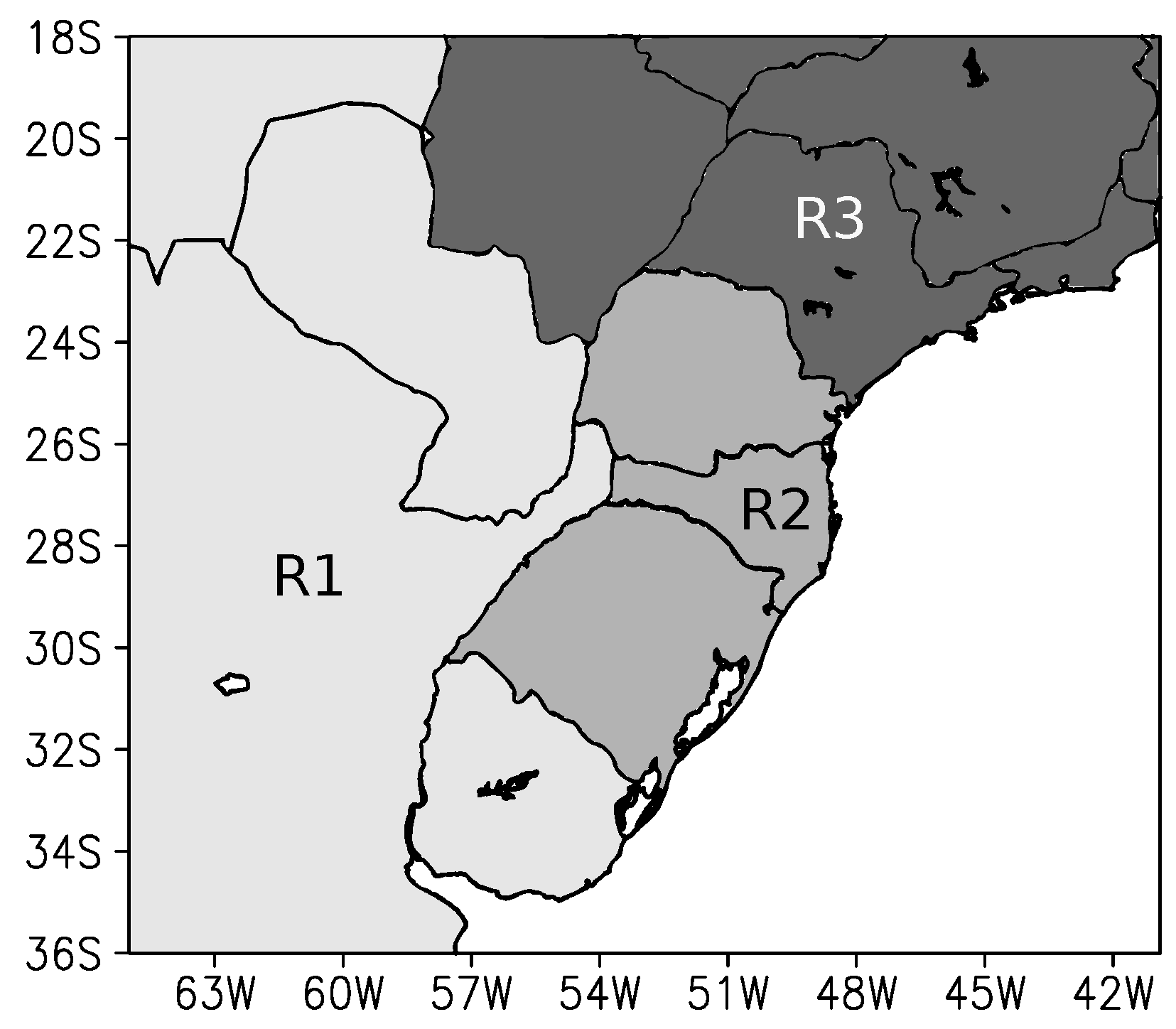
Figure 2.
Typical topology of a neural network.
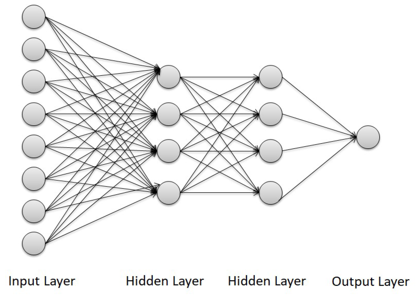
Figure 3.
Events of occurrence and non-occurrence of frosts for July 17, 2017.
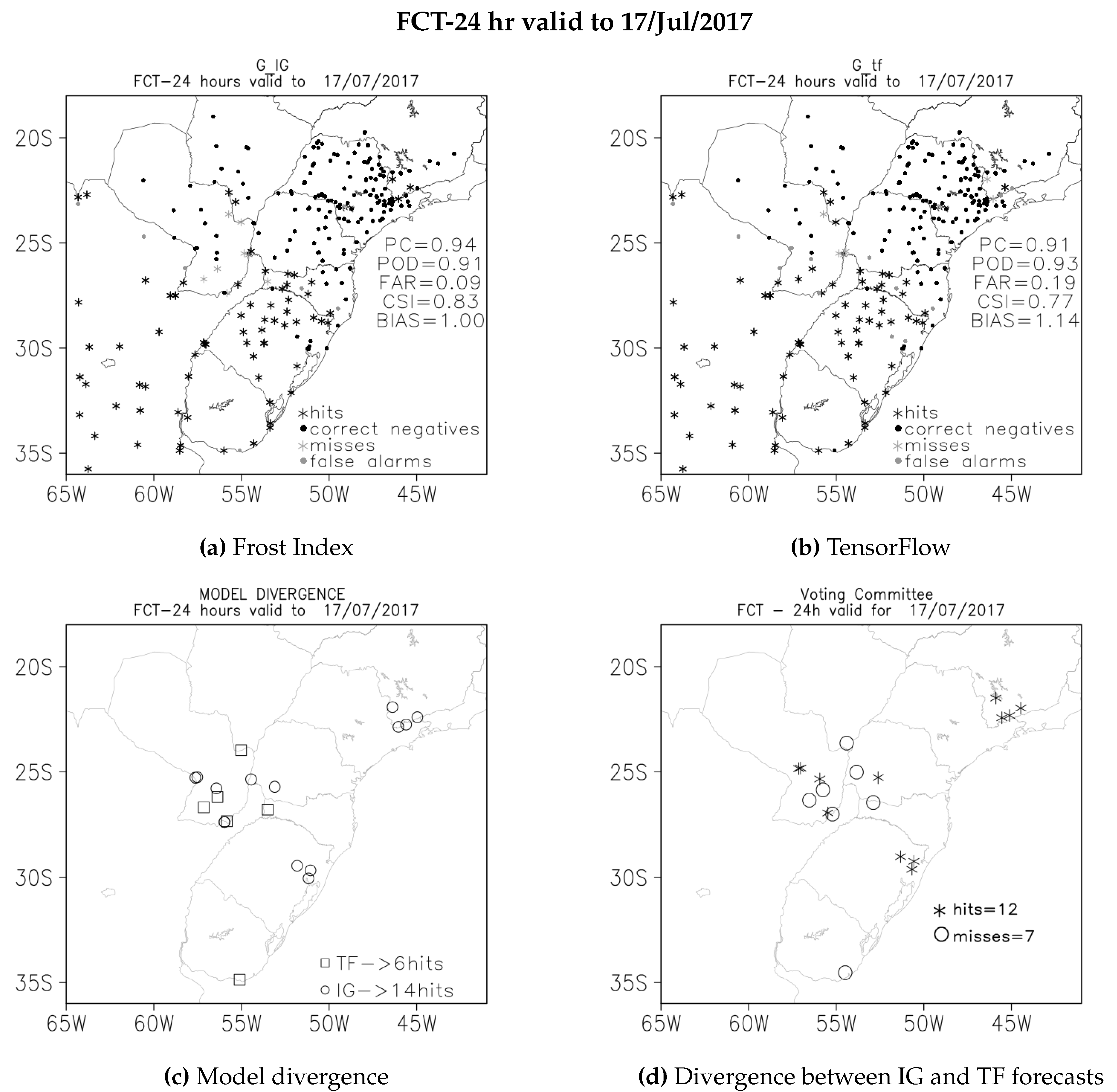
Figure 4.
Events of occurrence and non-occurrence of frosts for July 18, 2017.
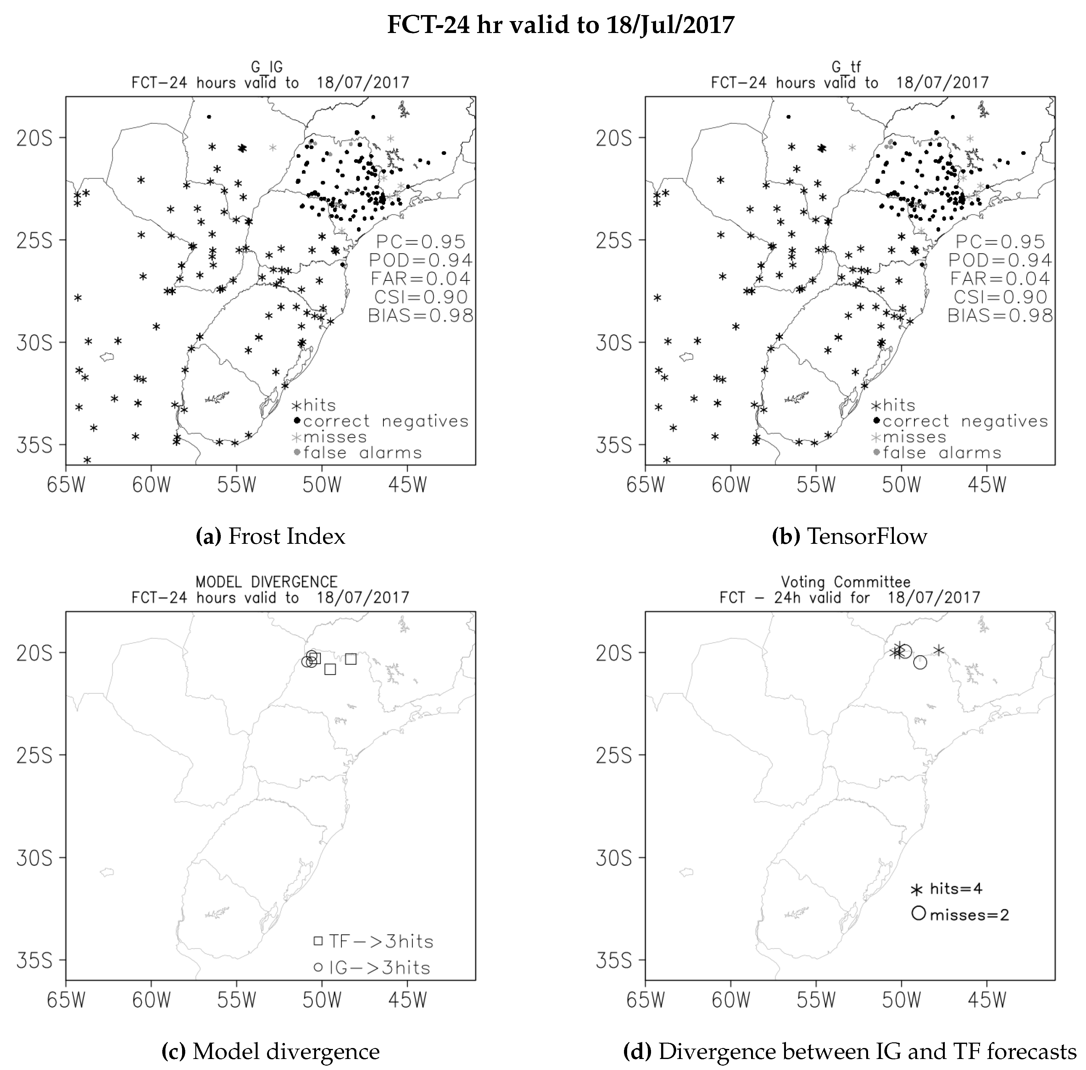
Figure 5.
Events of occurrence and non-occurrence of frosts for July 20, 2017.

Figure 6.
Events of occurrence and non-occurrence of frosts for July 21, 2017.
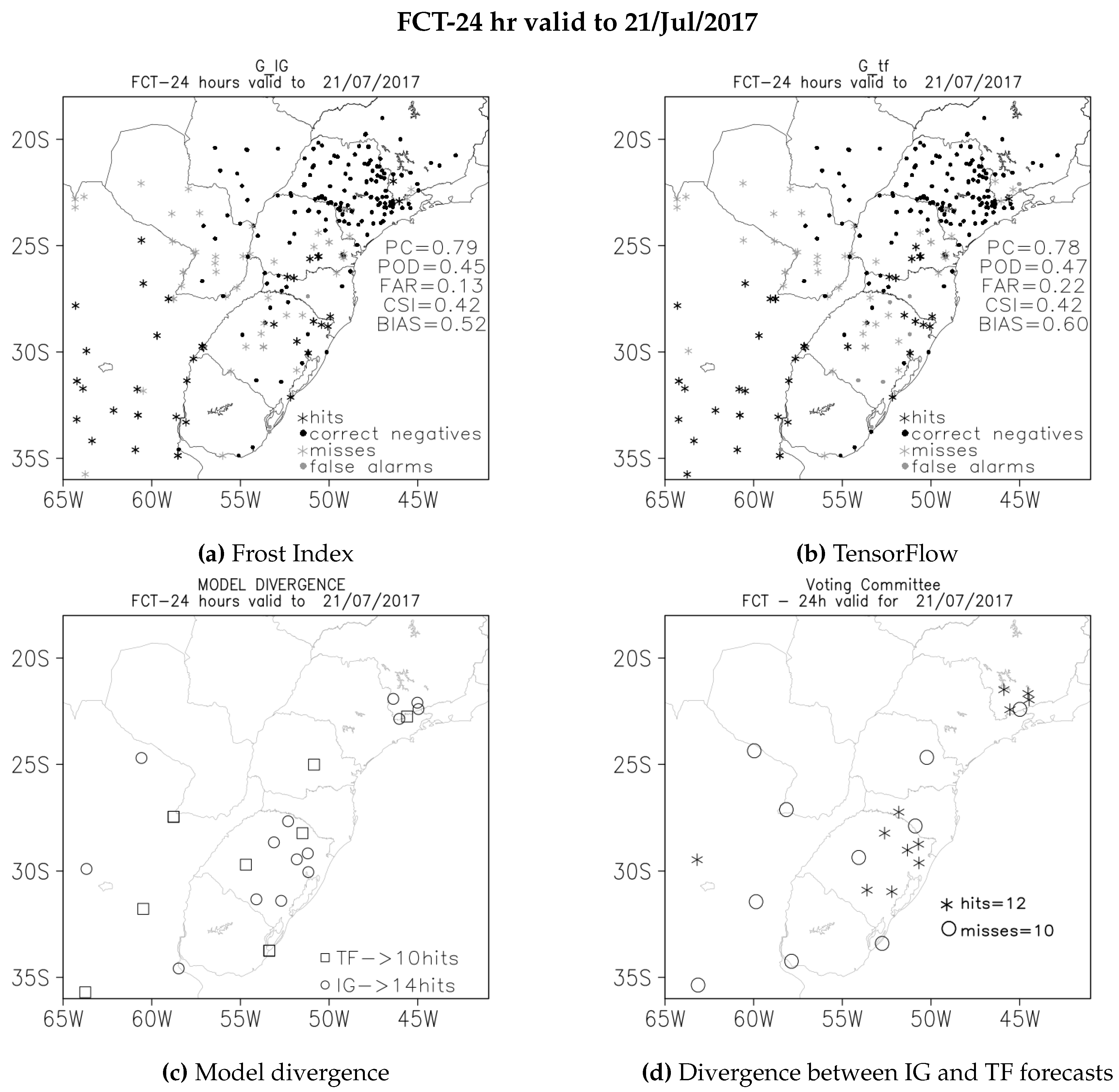
Figure 7.
Events of occurrence and non-occurrence of frosts for July 24, 2017.

Figure 8.
Events of occurrence and non-occurrence of frosts for May 21, 2018.
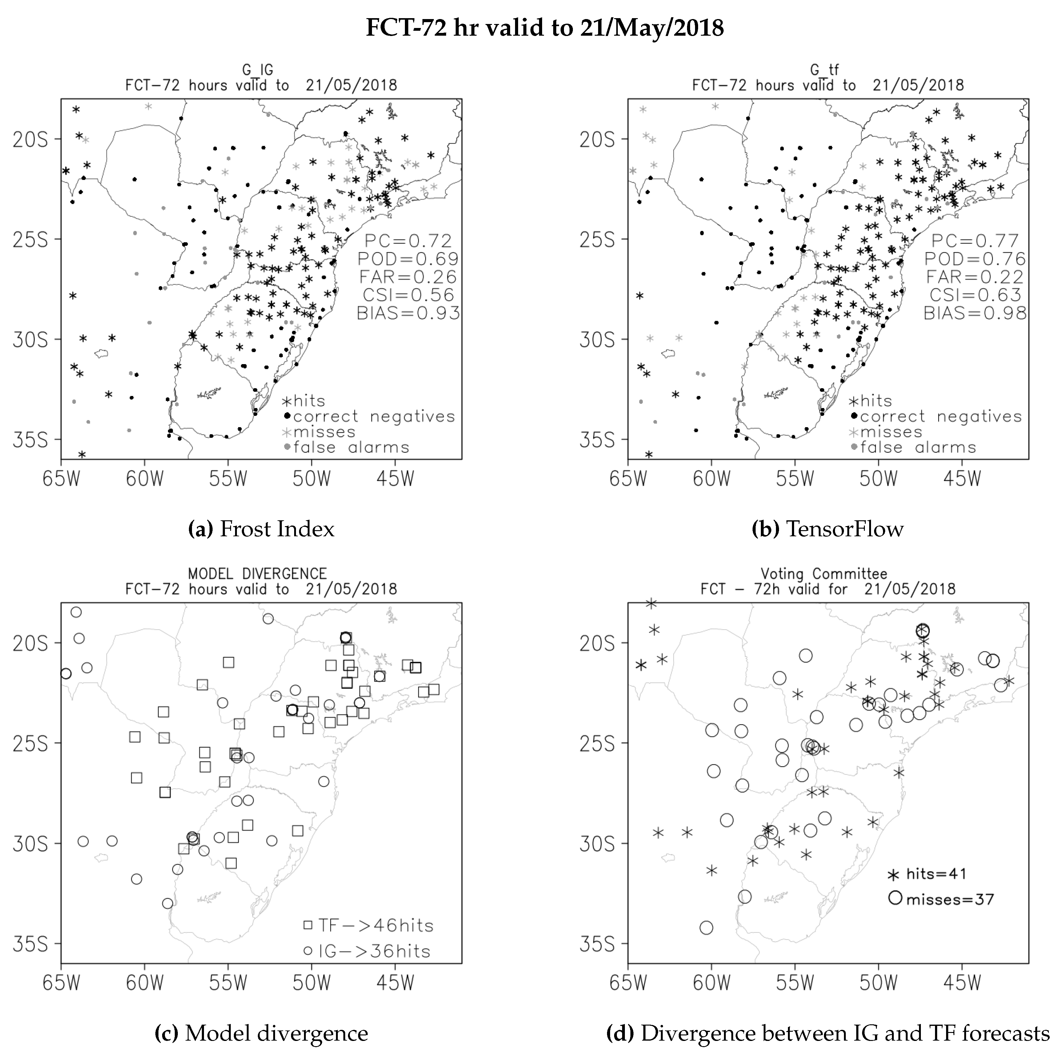

Table 1.
Statistical indices for evaluation.
| Index | Equation | Description | Reference Values |
|---|---|---|---|
| CSI | Proportion of hits excluding correctly "No" events forecasts | Perfect when 1 | |
| POD | Proportion of hits among observed "Yes" events | Perfect when 1 | |
| SR | Proportion of hits among forecasts "Yes" events | Perfect when 1 | |
| FAR | Proportion of misses of "Yes" events | Perfect when 0 | |
| Bias | Proportion of predicted events and observed events | Perfect when 1 |
Table 2.
Contingency table.
| Observed | |||
|---|---|---|---|
| Predicted | Yes | No | Total |
| Yes | a | b | a+b |
| No | c | d | c+d |
| Total | a+c | b+d | n=a+b+c+d |
Table 3.
Final topology and other characteristics of neural networks in TensorFlow experiment.
| Hyperparameters | NN-TensorFlow |
|---|---|
| Version | 2.0.0 |
| Number of Inputs | 7 |
| Number of Layers | 2 |
| Number of hidden units (each layer) | 25 |
| Activation function (hidden layers) | ReLU |
| Activation function (output) | sigmoid |
| Optimizer | Adam1 |
| Learning rate | 0.001 (default) |
| Momentum | 0.9 (default) |
| Epochs | 1000 |
Table 4.
Results.
| Date | Model | PC | POD | FAR | SR | CSI | BIAS |
|---|---|---|---|---|---|---|---|
| 2017071700 | IG | 0.94 | 0.91 | 0.09 | 0.91 | 0.83 | 1.00 |
| TF | 0.91 | 0.93 | 0.19 | 0.81 | 0.77 | 1.14 | |
| 2017071800 | IG | 0.95 | 0.94 | 0.04 | 0.96 | 0.90 | 0.98 |
| TF | 0.95 | 0.94 | 0.04 | 0.96 | 0.90 | 0.98 | |
| 2017072000 | IG | 0.82 | 0.70 | 0.14 | 0.86 | 0.62 | 0.81 |
| TF | 0.82 | 0.70 | 0.14 | 0.86 | 0.63 | 0.82 | |
| 2017072100 | IG | 0.79 | 0.45 | 0.13 | 0.87 | 0.42 | 0.52 |
| TF | 0.78 | 0.47 | 0.22 | 0.78 | 0.42 | 0.60 | |
| 2017072400 | IG | 0.95 | 0.42 | 0.50 | 0.50 | 0.29 | 0.83 |
| TF | 0.95 | 0.58 | 0.56 | 0.44 | 0.33 | 1.33 |
Table 5.
Results ondivergence.
| Date | Class | PC | POD | FAR | SR | CSI | BIAS |
|---|---|---|---|---|---|---|---|
| 2017071700 | frost | 0.55 | 0.13 | 0.67 | 0.33 | 0.10 | 0.38 |
| no frost | 0.55 | 0.83 | 0.41 | 0.59 | 0.53 | 1.42 | |
| 2017071800 | frost | 0.67 | 0.00 | 1.00 | 0.00 | 0.00 | 0.00 |
| no frost | 0.67 | 0.67 | 0.00 | 1.00 | 0.67 | 0.67 | |
| 2017072000 | frost | 0.29 | 0.31 | 0.60 | 0.40 | 0.21 | 0.77 |
| no frost | 0.29 | 0.25 | 0.82 | 0.18 | 0.12 | 1.38 | |
| 2017072100 | frost | 0.50 | 0.36 | 0.38 | 0.63 | 0.29 | 0.57 |
| no frost | 0.50 | 0.70 | 0.56 | 0.44 | 0.37 | 1.60 | |
| 2017072400 | frost | 0.50 | 0.00 | 1.00 | 0.00 | 0.00 | 2.50 |
| no frost | 0.50 | 0.58 | 0.22 | 0.78 | 0.50 | 0.75 |
Table 6.
Results.
| Model | Region | CSI | POD | SR | FAR | BIAS |
|---|---|---|---|---|---|---|
| Frost Index | R1 | 0.68 | 0.72 | 0.82 | 0.18 | 0.88 |
| Tensorflow | R1 | 0.60 | 0.68 | 0.84 | 0.16 | 0.81 |
| Frost Index | R2 | 0.57 | 0.69 | 0.77 | 0.23 | 0.90 |
| Tensorflow | R2 | 0.54 | 0.71 | 0.70 | 0.30 | 1.01 |
| Frost Index | R3 | 0.38 | 0.52 | 0.58 | 0.42 | 0.89 |
| Tensorflow | R3 | 0.36 | 0.52 | 0.53 | 0.47 | 0.99 |
Table 7.
Results on divergence.
| Class | Region | PC | POD | FAR | SR | CSI | BIAS |
|---|---|---|---|---|---|---|---|
| Frost | R1 | 0.55 | 0.65 | 0.40 | 0.60 | 0.45 | 1.08 |
| No Frost | R1 | 0.55 | 0.44 | 0.51 | 0.49 | 0.30 | 0.90 |
| Frost | R2 | 0.65 | 0.46 | 0.42 | 0.58 | 0.35 | 0.80 |
| No Frost | R2 | 0.65 | 0.78 | 0.32 | 0.68 | 0.57 | 1.14 |
| Frost | R3 | 0.65 | 0.55 | 0.54 | 0.46 | 0.33 | 1.21 |
| No Frost | R3 | 0.65 | 0.70 | 0.23 | 0.77 | 0.58 | 0.90 |
Disclaimer/Publisher’s Note: The statements, opinions and data contained in all publications are solely those of the individual author(s) and contributor(s) and not of MDPI and/or the editor(s). MDPI and/or the editor(s) disclaim responsibility for any injury to people or property resulting from any ideas, methods, instructions or products referred to in the content. |
© 2024 by the authors. Licensee MDPI, Basel, Switzerland. This article is an open access article distributed under the terms and conditions of the Creative Commons Attribution (CC BY) license (http://creativecommons.org/licenses/by/4.0/).
Copyright: This open access article is published under a Creative Commons CC BY 4.0 license, which permit the free download, distribution, and reuse, provided that the author and preprint are cited in any reuse.


