A Bivariate Extension of Type II Generalized Crack Distribution for Modelling Heavy-Tailed Losses

Preprint

Article

A Bivariate Extension of Type II Generalized Crack Distribution for Modelling Heavy-Tailed Losses

Altmetrics

Downloads

Views

Comments

A peer-reviewed article of this preprint also exists.

This version is not peer-reviewed

Submitted:

31 October 2024

Posted:

01 November 2024

You are already at the latest version

Alerts

Abstract

As an extension of the (univariate) Birnbaum-Saunders distribution, the Type II generalized crack (GCR2) distribution, built on an appropriate base density, provides a sufficient level of flexibility to fit various distributional shapes including heavy-tailed ones. In this paper, we develop a bivariate extension of the Type-II generalized crack distribution and study its dependency structure. For practical applications, several specific distributions, GCR2-Generalized Gaussian, GCR2-Student’s t and GCR2-Logistic, are constructed. The expectation-maximization algorithm is implemented to estimate the parameters in the bivariate GCR2 models. The model fitting results on the catastrophic loss dataset show that the bivariate GCR2 distribution base on the generalized Gaussian density fits the data significantly better than other alternative models.

Keywords:

Subject: Computer Science and Mathematics - Probability and Statistics

1. Introduction

Researchers have examined diverse classes of distributions to study various facets of problems. Most loss datasets in the context of actuarial loss modelling, share some common characteristics, such as being skewed to the right, unimodal in form (multimodal in certain situations), and having a thin left tail and a moderate to extremely thick right tail. In recent years, various classes of heavy-tailed distributions including the subexponential distribution class, have been studied for modelling heavy-tailed (or extreme) data ([1,2,3]). On the other hand, a different stream of problems, like the periodic vibrations in commercial aircraft, motivated the introduction of the Birnbaum-Saunders (BS) distribution ([4]). The BS distribution models the total time elapsed until a critical threshold is exceeded by fatigue accumulated on a subject of interest (material), causing the failure event of the material to occur. The BS distribution is a two-parameter lifespan distribution derived for material fatigue data modelling. Due to its ability to fit right-skewed data, it is highly effective for modelling numerous scenarios. For example, in situations where there is an accumulation of a certain factor that drives a quantifiable characteristic to surpass a critical threshold ([5]).

Various classes of extension of the BS distribution have been discussed in the literature. In [6], a type of generalized Birnbaum-Saunders distribution family that replaced the standard normal with elliptically contoured density functions is introduced. The extreme value version of the generalized Birnbaum-Saunders (GBS) distribution, which proved that the tail thickness of the auxiliary distribution (i.e., standard elliptically symmetric distribution) determines that of the GBS distribution, has been discussed in [7]. Some applications of the extreme value BS models can be found in [5,8].

Another important extension of the BS distribution is the three-parameter (Gaussian) crack distribution ([9]). The constructed distribution is a two-component mixture of inverse Gaussian and length-biased inverse Gaussian distributions with a weight parameter p. The Gaussian crack distribution features increased flexibility to fit various datasets due to the additional the mixture weight parameter. However, the thin-tailedness of standard normal base density imposes restrictions on the Gaussian crack distribution when it comes to modelling heavy-tailed data. Due to the importance of the heavy-tailed distributions and extension to various applications beyond reliability theory and survival analysis, researchers looked for new statistical distributions. The introduction of heavy-tailed distributions with additional parameters addresses the shortcomings of the traditional distributions. A notable extension by [10] results in a large class of generalized crack (GCR) distributions, which contains the three-parameter Gaussian crack (lifetime) distribution as a specific member. Each member of the generalized crack distribution class is built on a specific choice of a base density function that determines the tail characteristics of the resulting GCR distribution. In [10,11], applications of GCR distributions built on the Student’s t and the generalized Gaussian base density functions to catastrophic losses and heavy-tailed precipitation time series, respectively, are given. The GCR distribution class has recently been further extended to the class of Type II generalized crack (GCR2) distribution ([12]) in which an additional shape parameter

τ

is included to increase flexibility over the GCR class. The tail characteristics of the base density function and the new shape parameter in the GCR2 model determine the right tail properties of the GCR2 class.

Regarding applications for bivariate data with heavy-tailed marginals, a bivariate GCR distribution with a form of four-component mixture of independent models, has been constructed in [13]. The authors demonstrate that bivariate GCR models can exhibit various dependence structures and serve as valuable models for various real-world situations.

This paper aims to extend the univariate GCR2 models to bivariate cases by employing the mixture model structure used in [13]. This study considers three specific examples of GCR2 distributions, a newly constructed GCR2 model based on the logistic density in addition to the two GCR2 models introduced in [12], to effectively fit insurance and catastrophic losses. This paper studies some theoretical properties of the constructed model such as conditional distribution and the measures of dependency (e.g., Spearman’s rho and Kendall’s tau), a method for model parameter estimation through the Expectation-Maximization (EM) algorithm, and fitting the model to natural disasters datasets to demonstrate its applicability.

The rest of this paper is organized as follows. Section 2 gives a brief review of the origin, definition, examples, and key properties of the univariate Type II generalized crack distributions for the reader’s convenience. In Section 3, the bivariate Type-II generalized crack distribution is introduced with some detailed discussions on its theoretical properties. A method of model estimation and its application on a real catastrophic loss dataset are presented in Section 4 and Section 5, respectively. Finally Section 6 provides some concluding comments.

2. Type-II Generalized Crack Distribution

2.1. Birnbaum-Saunders Distribution

Birnbaum-Saunders (BS) distribution (also known as the fatigue-life distribution) was motivated by the problem of periodic vibration in aircraft that caused the materials to fatigue [4]. The Birnbaum-Saunders distribution is a well-known distribution for modelling the time of a crack (or a failure) happening when a material specimen is used repeatedly and experiences material fatigue due to gradual accumulation of stress/damages. The failure event occurs when the accumulated stress on the material specimen hits a critical threshold

w > 0

and the failure time T is the first hitting time of the accumulated stress to the critical threshold. Details of the Birnbaum-Saunders setting based on Brownian motion can be found in [12]. The Birnbaum-Saunders distribution is known to be a two-point mixture of the inverse Gaussian (IG) and the length-biased inverse Gaussian (LB-IG) distributions with equal mixture weights. Specifically the cumulative distribution function (cdf) and probability density function (pdf) of the BS distribution are as follows respectively:

\begin{matrix} F_{B S} (t; α, β) = Φ (\frac{1}{α} (\sqrt{\frac{t}{β}} - \sqrt{\frac{β}{t}})), t > 0, \end{matrix}

(1)

\begin{matrix} f_{B S} (t; α, β) = \frac{1}{2} f_{I G} (x; α, β) + \frac{1}{2} f_{L B - I G} (t; α, β), t > 0 \end{matrix}

(2)

where

\begin{matrix} f_{I G} (t; α, β) & = & \frac{\sqrt{β}}{α} t^{- 3 / 2} ϕ [\frac{1}{α} \{{(\frac{t}{β})}^{1 / 2} - {(\frac{β}{t})}^{1 / 2}\}] \end{matrix}

(3)

\begin{matrix} f_{L B - I G} (t; α, β) & = & \frac{1}{α \sqrt{β}} t^{- 1 / 2} ϕ [\frac{1}{α} \{{(\frac{t}{β})}^{1 / 2} - {(\frac{β}{t})}^{1 / 2}\}] \end{matrix}

(4)

Here

β > 0

and

α > 0

are the scale and shape parameters, respectively.

Φ (\cdot)

and

ϕ (\cdot)

denote the cdf and pdf of the standard normal distribution, whereas

f_{I G}

and

f_{L B - I G}

denotes the cdf and pdf of the two-parameter IG and the LB-IG distributions, respectively.

2.2. Gaussian Crack (CR) Distribution

The Gaussian crack distribution ([9]) is an extension of BS distribution by introducing the weight parameter

p \in [0, 1]

in place of the fixed weight of 1/2 in the BS distribution. Naturally the CR distribution allows for higher flexibility compared to the classical BS distribution. The pdf of the Gaussian crack (CR) distribution is given as follows:

\begin{matrix} f_{C R} (t; α, β, p) & = & p f_{I G} (t; α, β) + q f_{L B - I G} (t; α, β) \\ = & (p \frac{\sqrt{β}}{α} t^{- 3 / 2} + (1 - p) \frac{1}{α \sqrt{β}} t^{- 1 / 2}) ϕ [\frac{1}{α} \{{(\frac{t}{β})}^{1 / 2} - {(\frac{β}{t})}^{1 / 2}\}], t > 0, \end{matrix}

where

β > 0

α > 0

and

0 \leq p \leq 1

are the scale, shape and mixture weight parameters, respectively, and

q = 1 - p

Despite the fact that the right tail of the CR distribution thickens as p decreases, the tail maintains the shape of an exponential distribution. It is easy to see that the limit of the hazard rate function of the crack distribution converges to a constant that is greater than zero, i.e.,

lim_{t \to \infty} \frac{f_{C R} (t)}{1 - F_{C R} (t)} = \frac{1}{2 β α^{2}} > 0,

which suggests that the Gaussian crack distribution does not belong to heavy-tailed distribution class ([3,14]).

2.3. Generalized Crack Distribution

In [10], the Gaussian CR distribution family has been extended to a large class of generalized crack (GCR) distribution whose members depend on the specification of base density function

g (\cdot)

, where

g (\cdot)

is a base (or auxiliary) density function which is symmetric about zero. The base density function replaces the standard normal density function

ϕ (\cdot)

used for the Gaussian crack density.

Specifically, a random variable T has the generalized crack(GCR) distribution with base density g, denoted as

G C R (α, β, p; g)

where the parameters

α > 0

β > 0

and the mixture weight

0 \leq p \leq 1

, if its pdf is given as: PDF of GCR:

\begin{matrix} f_{G C R} (t; α, β, p; g) = p f_{I S} (t; α, β; g) + q f_{L B - I S} (t; α, β; g) \end{matrix}

where

\begin{matrix} f_{I S} (t; α, β) & = & \frac{\sqrt{β}}{α} t^{- 3 / 2} g [\frac{1}{α} \{{(\frac{t}{β})}^{1 / 2} - {(\frac{β}{t})}^{1 / 2}\}] \\ f_{L B - I S} (t; α, β) & = & \frac{1}{α \sqrt{β}} t^{- 1 / 2} g [\frac{1}{α} \{{(\frac{t}{β})}^{1 / 2} - {(\frac{β}{t})}^{1 / 2}\}] \end{matrix}

Here,

f_{I S}

and

f_{L B - I S}

are referred to as the pdfs of the inverse symmetric (IS) and the length-biased inverse symmetric (LB-IS) distribution, respectively, on the base density function

g (\cdot)

. The cdf of the

G C R (α, β, p; g)

distribution is given as:

\begin{matrix} F_{G C R}^{g} (t; α, β, p) = \bar{G} (b (t)) + (2 p - 1) \int_{\sqrt{s^{2} + 4 / α^{2}}}^{\infty} g (\sqrt{x^{2} - \frac{4}{α^{2}}}) d x \end{matrix}

where

\bar{G} (\cdot) = 1 - G (\cdot)

G (\cdot)

is the distribution function of base density function

g (\cdot)

, and

b (t) = \frac{1}{α} [\sqrt{t / β} - \sqrt{β / t}]

A general expression for the nth raw moments of the IS and LB-IS random variable along with details on the tail behaviour of the GCR distribution is provided in [10]. Their findings demonstrated that, with an appropriate choice of base density function, the heavy-tailed generalized crack distribution performs better than many well-known parametric distributions, such as Log-normal, Pareto type II, and Weibull distributions, which are frequently used in modelling positively skewed and heavy-tailed extreme data sets.

2.4. Type-II Birnbaum-Saunders (BS2) Distribution

The type-II Birnbaum-Saunders distribution extends the BS distribution by introducing another shape parameter

τ

. Applying the inverse transform method to Eq. 1, it can easily be verified that the following stochastic relationship holds. Let us define a random variable T as

T = β {(\frac{α X + \sqrt{α^{2} X^{2} + 4}}{2})}^{2}

where X is a standard normal random variable. The Type-II Birnbaum-Saunders (BS2) distribution introduces an additional shape parameter

τ > 0

to the expression above, defined formally as

T = β {(\frac{α X + \sqrt{α^{2} X^{2} + 4}}{2})}^{1 / τ} .

The pdf of the Type-II Birnbaum-Saunders (BS2) distribution is

\begin{matrix} f_{B S 2} (x; α, β, τ) & = & (\frac{2 τ}{α β}) [\frac{1}{2} {(\frac{β}{x})}^{τ + 1} + \frac{1}{2} {(\frac{x}{β})}^{τ - 1}] ϕ [\frac{1}{α} \{{(\frac{x}{β})}^{τ} - {(\frac{β}{x})}^{τ}\}] \\ = & \frac{1}{2} f_{B S 2}^{(1)} (x; α, β, τ) + \frac{1}{2} f_{B S 2}^{(2)} (x; α, β, τ), \end{matrix}

where

α > 0, β > 0, τ > 0

are model parameters, and

\begin{matrix} f_{B S 2}^{(1)} (x; α, β, τ) & = & (\frac{2 τ}{α β}) {(\frac{β}{x})}^{τ + 1} ϕ [\frac{1}{α} \{{(\frac{x}{β})}^{τ} - {(\frac{β}{x})}^{τ}\}] \\ f_{B S 2}^{(2)} (x; α, β, τ) & = & (\frac{2 τ}{α β}) {(\frac{x}{β})}^{τ - 1} ϕ [\frac{1}{α} \{{(\frac{x}{β})}^{τ} - {(\frac{β}{x})}^{τ}\}] . \end{matrix}

The cdf is given as

\begin{matrix} F_{B S 2} (x; α, β, τ) = Φ [\frac{1}{α} \{{(\frac{x}{β})}^{τ} - {(\frac{β}{x})}^{τ}\}] . \end{matrix}

(5)

Like the BS distribution, the BS2 distribution is a two-point mixture of densities

f_{B S 2}^{(1)}

and

f_{B S 2}^{(2)}

having equal weights. However, with the extra shape parameter

τ

, the BS2 distribution provides more flexibility over the BS distribution. The BS2 distribution reduces to the Birnbaum-Saunders distribution when

τ = 1 / 2

2.5. Type-II Generalized Crack Distribution

The Type-II generalized crack distribution class can be seen as a natural extension of the Type-II Birnbaum-Saunders distribution by replacing the standard normal density with a symmetric base density and including the mixture weight parameter p ([12]). Specifically the pdf of GCR2 distribution with base density g is given as follows:

\begin{matrix} f_{G C R 2} (x; α, β, τ, p; g) = p f_{G C R 2}^{(1)} (x; α, β, τ; g) + q f_{G C R 2}^{(2)} (x; α, β, τ; g) \end{matrix}

where

\begin{matrix} f_{G C R 2}^{(1)} (x; α, β, τ; g) & = & (\frac{2 τ}{α β}) {(\frac{β}{x})}^{τ + 1} g [\frac{1}{α} \{{(\frac{x}{β})}^{τ} - {(\frac{β}{x})}^{τ}\}] \\ f_{G C R 2}^{(2)} (x; α, β, τ; g) & = & (\frac{2 τ}{α β}) {(\frac{x}{β})}^{τ - 1} g [\frac{1}{α} \{{(\frac{x}{β})}^{τ} - {(\frac{β}{x})}^{τ}\}] . \end{matrix}

Respectively the cdf of GCR2 distribution with base density g is given as

\begin{matrix} F_{G C R 2} (x; α, β, τ, p; g) = p F_{G C R 2}^{(1)} (x; α, β, τ; g) + q F_{G C R 2}^{(2)} (x; α, β, τ; g) \end{matrix}

where

\begin{matrix} F_{G C R 2}^{(1)} (x; α, β, τ; g) & = & \int_{b (x)}^{\infty} g (s) (1 + \frac{s}{\sqrt{s^{2} + 4 / α^{2}}}) d s \\ F_{G C R 2}^{(2)} (x; α, β, τ; g) & = & \int_{b (x)}^{\infty} g (s) (1 - \frac{s}{\sqrt{s^{2} + 4 / α^{2}}}) d s, \end{matrix}

and

b (x) : = b (x; α, β, τ) = α^{- 1} [{(β / x)}^{τ} - {(x / β)}^{τ}]

2.6. Specific Examples of GCR2 Distributions

The specification of the base density function on which GCR2 distribution is built may depend on some key distributional features (such as tail characteristics) that are required for each specific application. Two practical examples, the GCR2-t and the GCR2-GG distributions whose base densities are the Student’s t and the generalized Gaussian (normal) distributions, respectively, are given in [12]. In this paper we also consider the GCR2 distribution with the logistic base density, referred to as the GCR2-LG distribution, as another member of the GCR2 distribution class.

Example 2.1.(GCR2-t distribution).

The Student’s t distribution has a regular varying tail and its density function is given as

g_{t} (x; ν) = \frac{Γ (\frac{ν + 1}{2})}{\sqrt{ν π} Γ (\frac{ν}{2})} {(1 + \frac{x^{2}}{ν})}^{- (\frac{ν + 1}{2})}, ν > 0 .

The corresponding density of the GCR2-t can be easily expressed as

\begin{matrix} f_{GCR 2}^{t} (t; α, β, τ, p; ν) & = & \frac{2 τ Γ (\frac{ν + 1}{2})}{α β \sqrt{ν π} Γ (\frac{ν}{2})} [p {(\frac{β}{t})}^{τ + 1} + q {(\frac{t}{β})}^{τ - 1}] \\ \times & {[1 + \frac{1}{α^{2} ν} {{(\frac{t}{β})}^{2 τ} + {(\frac{β}{t})}^{2 τ} - 2}]}^{- (\frac{ν + 1}{2})} . \end{matrix}

The Student’s t distribution belongs to the Maximum Domain of Attraction (MDA) of the Fréchet distribution with index

ν

, which means that the distribution of a properly normalized maximum of independent and identically distributed (i.i.d.) Student’s t random variables converge to a Fréchet distribution asymptotically. Bae and Volodin[12] show that the tail of the GCR2-t distribution is regular varying with index

τ

ν

, and thus it also belongs to the MDA of the Fréchet distribution. Comparing with the tail of the GCR-t distribution that has the index

\frac{1}{2}

ν

, the tail of GCR2-t becomes heavier than that of the GCR-t when

τ

gets smaller than

1 / 2

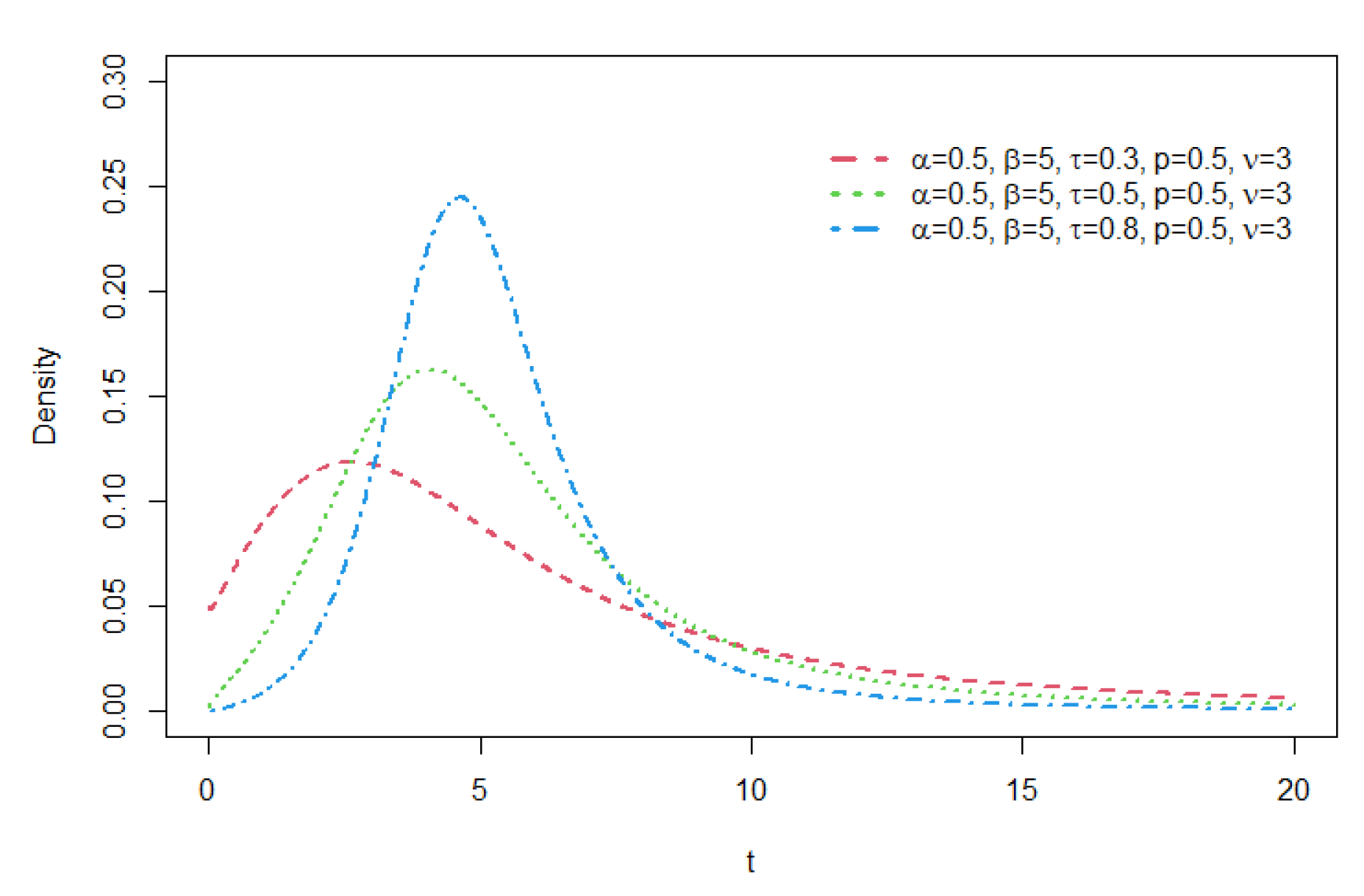
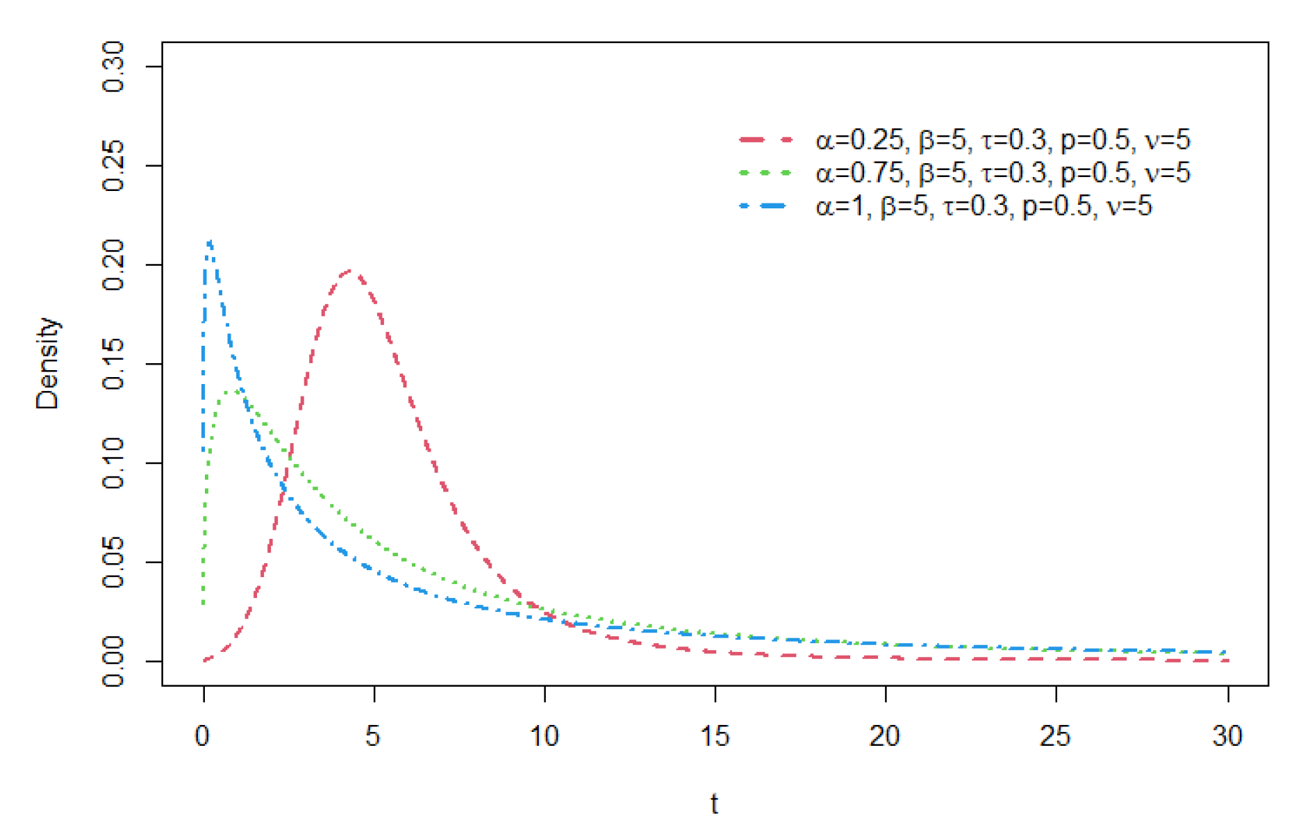
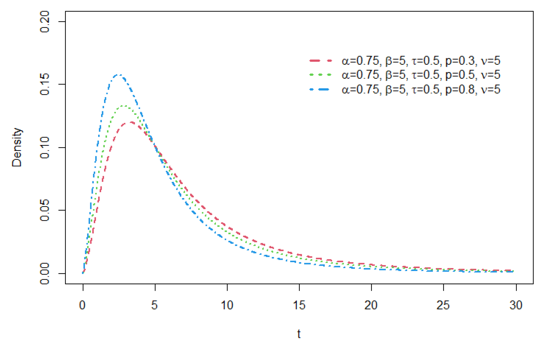
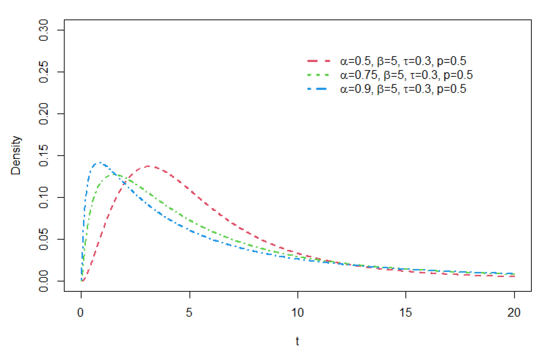
. Figure 1, Figure 2 and Figure 3 illustrate the shapes of the GCR2-t density function for a few prescribed parameter sets.

Example 2.2. (GCR2-GG distribution).

The GCR2-GG is a large distribution family which encompasses both thin to moderately heavy-tailed ones, and it can be useful for various practical applications. In particular when

θ < 1

, the generalized Gaussian model is subexponential ([3]). The pdf of the Generalized Gaussian (GG) is given as

g_{GG} (x; θ) = \frac{θ}{2 λ Γ (\frac{1}{θ})} exp (- {|\frac{x - μ}{λ}|}^{θ}) .

For symmetry, we set

μ = 0

and, for the identification of parameters, we set

λ = \sqrt{Γ (1 / θ) / Γ (3 / θ)}

. The density function of the resulting GCR2-GG distribution has the following expression:

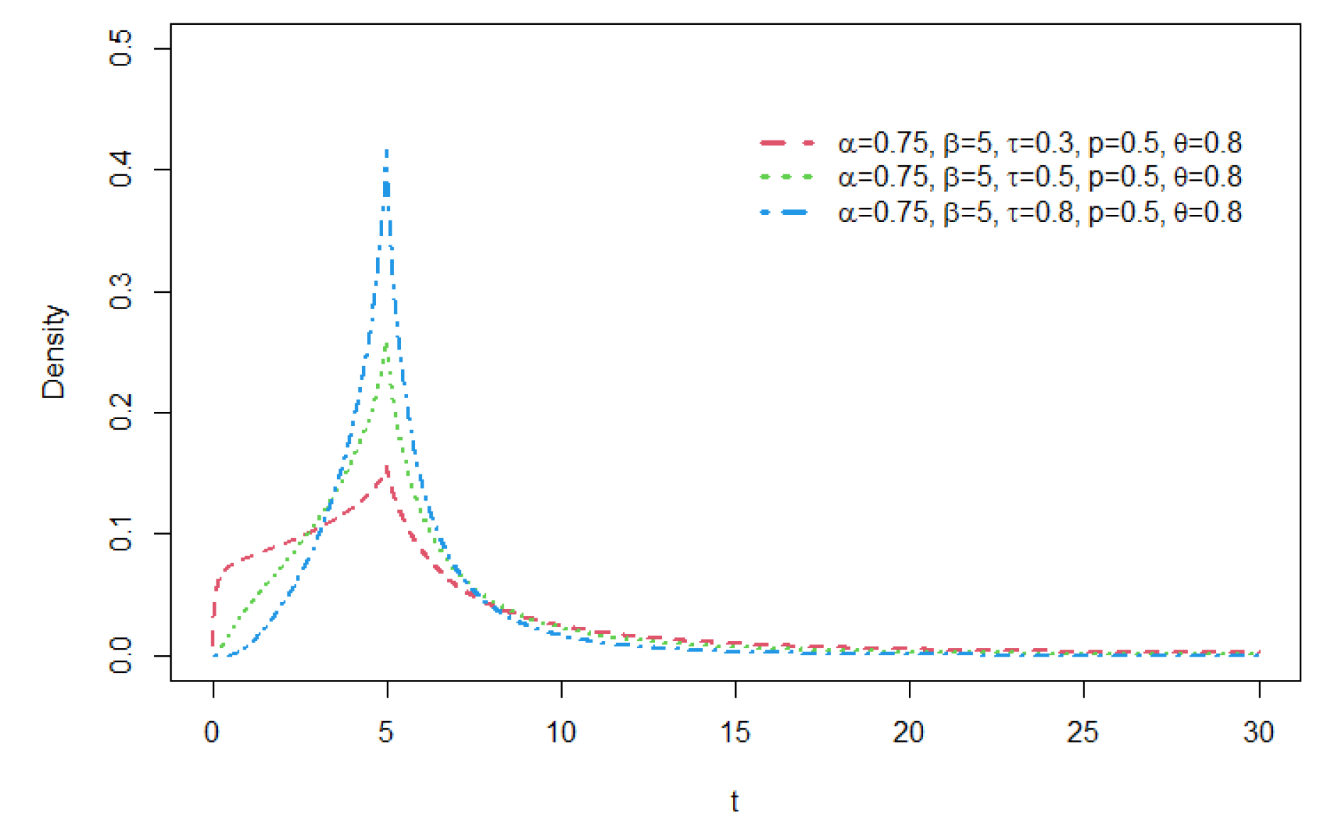
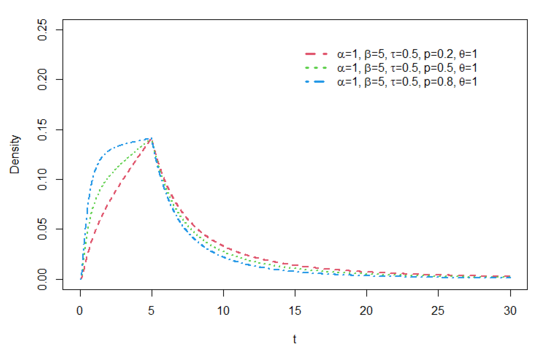
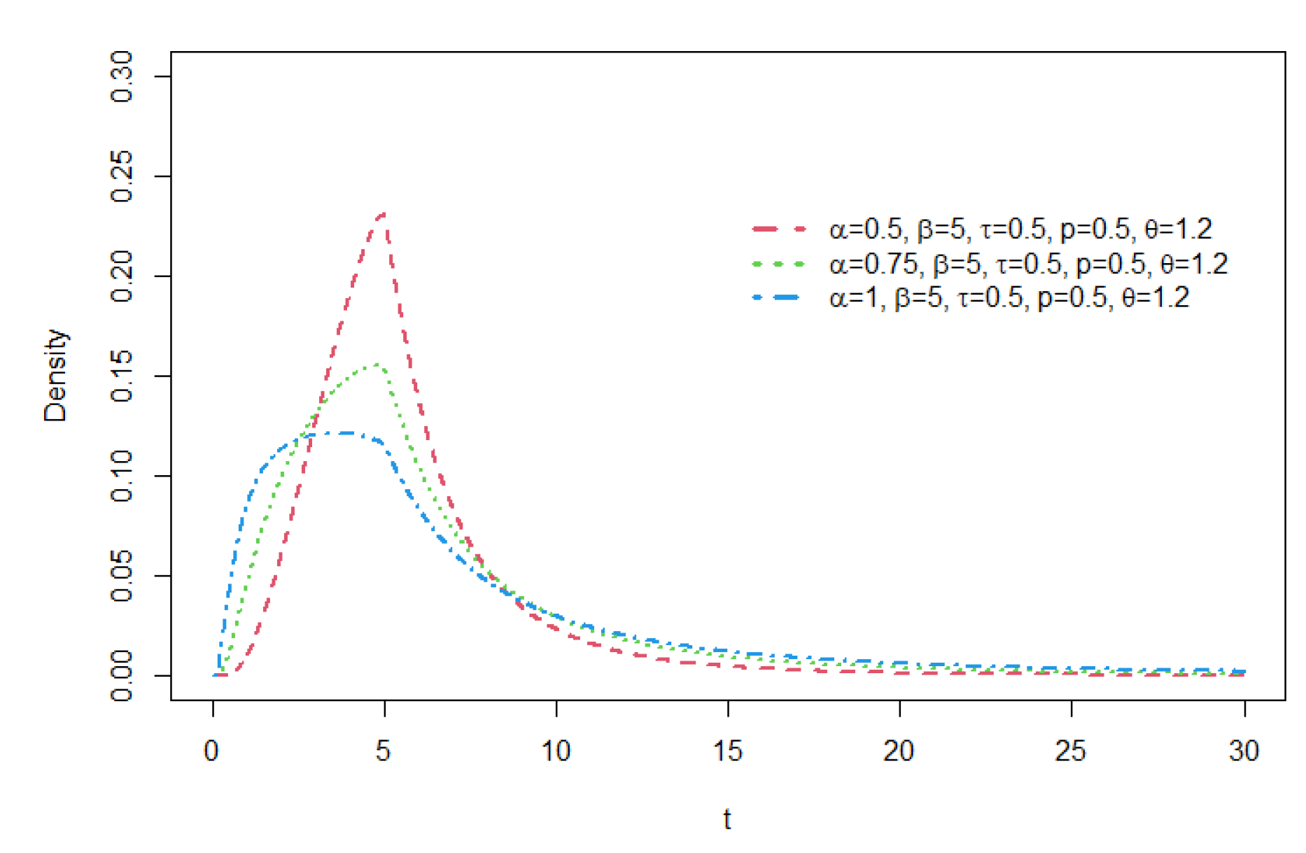
\begin{matrix} f_{GCR 2}^{GG} (t; α, β, τ, p; θ) & = & \frac{τ θ}{α β λ Γ (\frac{1}{θ})} [p {(\frac{β}{t})}^{τ + 1} + q {(\frac{t}{β})}^{τ - 1}] \\ \times & exp (- {|\frac{1}{α λ} [{(\frac{t}{β})}^{τ} - {(\frac{β}{t})}^{τ}]|}^{θ}) . \end{matrix}

Figure 4 – Figure 6 illustrate the shapes of the GCR2-GG density function for a few prescribed parameter sets.

Example 2.3. (GCR2-LG distribution).

The Logistic (LG) distribution has the density function

g_{LG} (x) = \frac{e^{- x / s}}{s {(1 + e^{- x / s})}^{2}} .

For the identification of parameters, we set

s = \frac{\sqrt{3}}{π}

. The resulting GCR2-LG distribution has the density function as follows:

\begin{matrix} f_{GCR 2}^{LG} (t; α, β, τ, p) & = & (\frac{2 τ}{α s β}) [p {(\frac{β}{t})}^{τ + 1} + q {(\frac{t}{β})}^{τ - 1}] \\ \times & \frac{exp {- \frac{1}{α s} [{(\frac{t}{β})}^{τ} - {(\frac{β}{t})}^{τ}]}}{{(1 + exp {- \frac{1}{α s} [{(\frac{t}{β})}^{τ} - {(\frac{β}{t})}^{τ}]})}^{2}} . \end{matrix}

The GCR2-LG distribution can be an effective model to fit thin to moderate-tailed datasets for financial and insurance applications and, with one less paramter, it is simpler than the GCR2-t and GCR2-GG distributions.

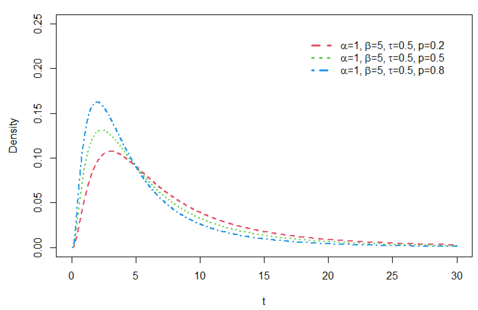
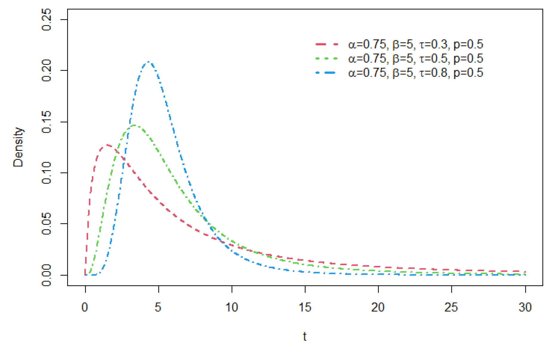
Figure 7 – Figure 9 illustrate the shapes of the GCR2-LG density function for a few prescribed parameter sets.

As seen from these figures, various distribution forms can be constructed depending on the distributional features of the base density function and the related shape parameters. For a GCR2 distribution family with a specific base density, the right tail of the distribution becomes heavier as the mixture weight parameter p gets smaller. The larger the shape parameter

α

is, the heavier the tail becomes, and the opposite is true for the shape parameter

τ

. For details of tail properties of the GCR2 distribution, see Theorem 1 and Theorem 2 in Bae and Volodin[12].

3. Bivaraite GCR2 Distribution

We introduce a bivariate extension of the Type II generalized crack distribution and study some properties like the conditional distribution and measures of association. Let g be a probability density function symmetric about zero. For two positive random variables, we define the bivariate Type-II generalized crack distribution as follows.

Definition 1.

A pair of random variables

T = (T_{1}, T_{2})

with base density g and parameters

α

α_{1}, α_{2}

β

= (

β_{1}, β_{2}

τ

= (

τ_{1}, τ_{2}

) and

p =

(

p_{11}, p_{12}, p_{21}, p_{22}

), has a bivariate Type-II generalized crack distribution, denoted as BVGCR2(

α

β

τ

,p;g), if and only if its joint pdf is given as follows:

\begin{matrix} f_{B V G C R 2} (t_{1}, t_{2}; α, β, τ, p; g) & = & p_{11} f_{G C R 2}^{(1)} (t_{1}; α_{1}, β_{1}, τ_{1}; g) f_{G C R 2}^{(1)} (t_{2}; α_{2}, β_{2}, τ_{2}; g) \\ + & p_{12} f_{G C R 2}^{(1)} (t_{1}; α_{1}, β_{1}, τ_{1}; g) f_{G C R 2}^{(2)} (t_{2}; α_{2}, β_{2}, τ_{2}; g) \\ + & p_{21} f_{G C R 2}^{(2)} (t_{1}; α_{1}, β_{1}, τ_{1}; g) f_{G C R 2}^{(1)} (t_{2}; α_{2}, β_{2}, τ_{2}; g) \\ + & p_{22} f_{G C R 2}^{(2)} (t_{1}; α_{1}, β_{1}, τ_{1}; g) f_{G C R 2}^{(2)} (t_{2}; α_{2}, β_{2}, τ_{2}; g), t_{1}, t_{2} > 0, \end{matrix}

where the mixture weight parameters satisfy

0 \leq p_{j} \leq 1

j \in J : = {11, 12, 21, 22}

\sum_{j \in J} p_{j} = 1

, and, for each

i = 1, 2,

\begin{matrix} f_{G C R 2}^{(1)} (t_{i}; α_{i}, β_{i}, τ_{i}; g) & = & (\frac{2 τ_{i}}{α_{i} β_{i}}) {(\frac{β_{i}}{t_{i}})}^{τ_{i} + 1} g [\frac{1}{α_{i}} \{{(\frac{t_{i}}{β_{i}})}^{τ_{i}} - {(\frac{β_{i}}{t_{i}})}^{τ_{i}}\}], \end{matrix}

and

\begin{matrix} f_{G C R 2}^{(2)} (t_{i}; α_{i}, β_{i}, τ_{i}; g) & = & (\frac{2 τ_{i}}{α_{i} β_{i}}) {(\frac{t_{i}}{β_{i}})}^{τ_{i} - 1} g [\frac{1}{α_{i}} \{{(\frac{t_{i}}{β_{i}})}^{τ_{i}} - {(\frac{β_{i}}{t_{i}})}^{τ_{i}}\}] . \end{matrix}

BVGCR2(

α

β

τ

,p;g) is a mixture of four combinations of independent bivariate distributions. It is easy to see that the marginal distributions of

T_{1}

and

T_{2}

are GCR2

(α_{1}, β_{1}, τ_{1}, p_{1} = p_{11} + p_{12}; g)

and GCR2

(α_{2}, β_{2}, τ_{2}, p_{2} = p_{11} + p_{21}; g)

, respectively. Note that, for simplicity, we assume that the marginal distributions are built based on the same base density function g whose model parameter can be distinct for each marginal.

We provide the conditional distribution which is an essential property for the simulation of the pair of random variables. Following the relationship between the two mixture components of the GCR2 distribution,

f_{G C R 2}^{(2)} (t; α, β, τ; g) / f_{G C R 2}^{(1)} (t; α, β, τ; g) = {(t / β)}^{2 τ}

, the conditional density of

T_{2}

given

T_{1} = t_{1}

is expressed as follows. For notational convenience, we drop subscript and the parameters in the functions and write as;

\begin{matrix} f_{2 | 1} (t_{2} | t_{1}; g) & : = \frac{p_{11} f^{(1)} (t_{1}; g) f^{(1)} (t_{2}; g) + p_{12} f^{(1)} (t_{1}; g) f^{(2)} (t_{2}; g)}{p_{1} f^{(1)} (t_{1}; g) + q_{1} f^{(2)} (t_{1}; g)} \\ + \frac{p_{21} f^{(2)} (t_{1}; g) f^{(1)} (t_{2}; g) + p_{22} f^{(2)} (t_{1}; g) f^{(2)} (t_{2}; g)}{p_{1} f^{(1)} (t_{1}; g) + q_{1} f^{(2)} (t_{1}; g)} \\ = \frac{p_{11} + p_{21} {(\frac{t_{1}}{β_{1}})}^{2 τ} f^{(1)} (t_{2}; g) + p_{12} + p_{22} {(\frac{t_{1}}{β_{1}})}^{2 τ} f^{(2)} (t_{2}; g)}{p_{1} + q_{1} {(\frac{t_{1}}{β_{1}})}^{2 τ}} \\ = (\frac{p_{11} + p_{21} {(\frac{t_{1}}{β_{1}})}^{2 τ}}{p_{1} + q_{1} {(\frac{t_{1}}{β_{1}})}^{2 τ}}) f^{(1)} (t_{2}; g) + (\frac{p_{12} + p_{22} {(\frac{t_{1}}{β_{1}})}^{2 τ}}{p_{1} + q_{1} {(\frac{t_{1}}{β_{1}})}^{2 τ}}) f^{(2)} (t_{2}; g) . \end{matrix}

Hence, the conditional distribution of

T_{2}

given

T_{1} = t_{1}

is also GCR2

(α_{2}, β_{2}, τ_{2}, p_{2 | 1}; g)

where,

p_{2 | 1} = \frac{p_{11} + p_{21} {(t_{1} / β_{1})}^{2 τ_{1}}}{p_{1} + q_{1} {(t_{1} / β_{1})}^{2 τ_{1}}} .

Using the conditional distribution, one can in sequence simulate the pairs of random variates

(T_{1}, T_{2})

for the BVGCR2 models, by first simulating

T_{1}

from the GCR2

(α_{1}, β_{1}, τ_{1}, p_{1}; g)

using the acceptance-rejection method as shown in Bae and Chen[10] and then, simulate

T_{2}

from the conditional distribution GCR2

(α_{2}, β_{2}, τ_{2}, p_{2 | 1}; g)

3.1. Dependence Measures

In this section we derive expressions for Spearman’s rho and Kendall’s tau of BVGCR2 random variables.

3.1.1. Spearman’s Rho

Spearman’s rho is a commonly used measure of association between two random variables. Due to the invariance under monotone transformations, Spearman’s rho provides a broad interpretation of the dependence structure for any bivariate distributions. With marginal densities,

f_{T_{1}} (t_{1})

and

f_{T_{2}} (t_{2})

for the random variables

T_{1}

and

T_{2}

, respectively, and the joint distribution

F (t_{1}, t_{2})

(t_{1}, t_{2}) \in R_{+}^{2}

, the (population version) Spearman’s rho is defined as;

\begin{matrix} ρ_{s} & = \frac{E (U_{1}, U_{2}) - E (U_{1}) E (U_{2})}{\sqrt{V a r (U_{1})} \sqrt{V a r (U_{2})}} \\ = 12 \int_{0}^{\infty} \int_{0}^{\infty} F (t_{1}, t_{2}) f_{T_{1}} (t_{1}) f_{T_{2}} (t_{2}) d t_{1} d t_{2} - 3 \end{matrix}

where

U_{1} = F_{T_{1}} (T_{1})

and

U_{2} = F_{T_{2}} (T_{2})

are uniform random variables. That is, Spearman’s rho is Pearson’s correlation between transformations of the variables into uniformly distributed ones. The following proposition provides an expression for Spearman’s rho of random variables having a BVGCR2 distribution.

Proposition 1.

Suppose

(T_{1}, T_{2}) \sim

BVGCR2(

α

β

τ

,p;g). Then, Spearman’s rho between

T_{1}

and

T_{2}

is given by

ρ_{s} = 48 (p_{11} p_{22} - p_{12} p_{21}) γ_{1} γ_{2},

(6)

where

γ_{i} = \int_{- \infty}^{\infty} \frac{t}{\sqrt{t^{2} + 4 / α_{i}^{2}}} G_{i} (t) g_{i} (t) d t, i = 1, 2 .

Proof. See Appendix A.

3.1.2. Kendall’s Tau

Kendall’s tau is a measure of concordance between two random variables. Formally, for the random variables

T_{1}

and

T_{2}

with the joint distribution

F (t_{1}, t_{2})

(t_{1}, t_{2}) \in R_{+}^{2}

, the (population-version) Kendall’s tau is defined as

\begin{matrix} τ_{k} & = P ((T_{1} - T_{1}^{'}) (T_{2} - T_{2}^{'}) > 0) - P ((T_{1} - T_{1}^{'}) (T_{2} - T_{2}^{'}) < 0) \\ = 4 \int_{0}^{\infty} \int_{0}^{\infty} F (t_{1}, t_{2}) f (t_{1}, t_{2}) d t_{1} d t_{2} - 1, \end{matrix}

where the pair

(T_{1}^{'}, T_{2}^{'})

has the joint distribution F and is independent to

(T_{1}, T_{2})

The following proposition provides an expression for Kendall’s tau of random variables having a BVGCR2 distribution.

Proposition 2.

Suppose

(T_{1}, T_{2}) \sim

BVGCR2(

α

β

τ

,p;g). Then , Kendall’s tau between

T_{1}

and

T_{2}

is given by

τ_{k} = 32 (p_{11} p_{22} - p_{12} p_{21}) γ_{1} γ_{2},

(7)

where

γ_{i} = \int_{- \infty}^{\infty} \frac{t}{\sqrt{t^{2} + 4 / α_{i}^{2}}} G_{i} (t) g_{i} (t) d t, i = 1, 2 .

Proof. See Appendix B.

Remark 3.1.

It is important to note that,

0 \leq γ \leq \frac{1}{4} .

(8)

This inequalities can be proven by using the symmetry of

g (t)

G (- t) = 1 - G (t)

and integration by parts. Specifically,

\begin{matrix} γ & = & \int_{- \infty}^{\infty} \frac{t}{\sqrt{t^{2} + 4 / α^{2}}} G (t) g (t) d t \\ = & \int_{- \infty}^{0} \frac{t}{\sqrt{t^{2} + 4 / α^{2}}} G (t) g (t) d t + \int_{0}^{\infty} \frac{t}{\sqrt{t^{2} + 4 / α^{2}}} G (t) g (t) d t \\ = & \int_{0}^{\infty} \frac{- s}{\sqrt{s^{2} + 4 / α^{2}}} G (- s) g (- s) d s + \int_{0}^{\infty} \frac{t}{\sqrt{t^{2} + 4 / α^{2}}} G (t) g (t) d t \\ = & - \int_{0}^{\infty} \frac{s}{\sqrt{s^{2} + 4 / α^{2}}} (1 - G (s)) g (s) d s + \int_{0}^{\infty} \frac{t}{\sqrt{t^{2} + 4 / α^{2}}} G (t) g (t) d t \\ = & - \int_{0}^{\infty} \frac{s}{\sqrt{s^{2} + 4 / α^{2}}} g (s) d s + 2 \int_{0}^{\infty} \frac{s}{\sqrt{s^{2} + 4 / α^{2}}} G (s) g (s) d s \\ = & \int_{0}^{\infty} (2 G (s) - 1) \frac{s}{\sqrt{s^{2} + 4 / α^{2}}} g (s) d s . \end{matrix}

For

0 < s < \infty

0 \leq 2 G (s) - 1 \leq 1

0 \leq \frac{s}{\sqrt{s^{2} + 4 / α^{2}}} \leq 1

, and applying integration by parts,

\begin{matrix} \int_{0}^{\infty} (2 G (s) - 1) \frac{s}{\sqrt{s^{2} + 4 / α^{2}}} g (s) d s & \leq & \int_{0}^{\infty} (2 G (s) - 1) g (s) d s \\ = & 1 - 2 \int_{0}^{\infty} G (s) g (s) d s = \frac{1}{4} . \end{matrix}

With this and by Eqs. (1) and (2), we obtain the following bounds for

ρ_{s}

and

τ_{k}

| ρ_{s} | \leq \frac{3}{4}, | τ_{k} | \leq \frac{1}{2},

Note that

ρ_{s}

and

τ_{k}

get the maximum when

p_{11}

p_{22}

=0.5 and

γ

attains its maximum of 1/4.

Also remark that, if

p_{11} p_{22} = p_{12} p_{21}

, and thus

ρ_{s} = τ_{k} = 0

, the joint density of the BVGCR2 model can be expressed as a product of two GCR2 marginals, i.e., the two random variables are independent.

3.2. Tail Independence

As remarked in the previous section, the dependency measures of the proposed BVGCR2 model are bounded, and thus the model may not be suitable for the cases where the extreme dependency is required, i.e., market turmoils. Here we further investigate the tail dependence of the BVGCR2 model in terms of the upper tail dependence which is defined as

\begin{matrix} λ_{U} = lim_{q \to 1} Pr [T_{1} > F_{T_{1}}^{- 1} (q) | T_{2} > F_{T_{2}}^{- 1} (q)] & = & lim_{q \to 1} \frac{Pr [T_{1} > F_{T_{1}}^{- 1} (q), T_{2} > F_{T_{2}}^{- 1} (q)]}{1 - q} \\ = & lim_{q \to 1} \frac{1 - 2 q + F_{T_{1}, T_{2}} (F_{T_{1}}^{- 1} (q), F_{T_{2}}^{- 1} (q))}{1 - q} \\ = & 2 - lim_{q \to 1} \frac{d}{d q} F_{T_{1}, T_{2}} (F_{T_{1}}^{- 1} (q), F_{T_{2}}^{- 1} (q)), \end{matrix}

(9)

where the last equality holds by the L’hospital’s rule. In fact,

\begin{matrix} \frac{d}{d q} F_{T_{1}, T_{2}} (F_{T_{1}}^{- 1} (q), F_{T_{2}}^{- 1} (q)) \\ = p_{11} \frac{d}{d q} \{F_{T_{1}}^{(1)} (F_{T_{1}}^{- 1} (q)) F_{T_{2}}^{(1)} (F_{T_{2}}^{- 1} (q))\} + p_{12} \frac{d}{d q} \{F_{T_{1}}^{(1)} (F_{T_{1}}^{- 1} (q)) F_{T_{2}}^{(2)} (F_{T_{2}}^{- 1} (q))\} \\ + p_{21} \frac{d}{d q} \{F_{T_{1}}^{(2)} (F_{T_{1}}^{- 1} (q)) F_{T_{2}}^{(1)} (F_{T_{2}}^{- 1} (q))\} + p_{22} \frac{d}{d q} \{F_{T_{1}}^{(2)} (F_{T_{1}}^{- 1} (q)) F_{T_{2}}^{(2)} (F_{T_{2}}^{- 1} (q))\} \\ = p_{11} \{F_{T_{2}}^{(1)} (F_{T_{2}}^{- 1} (q)) \frac{f_{T_{1}}^{(1)} (F_{T_{1}}^{- 1} (q))}{f_{T_{1}} (F_{T_{1}}^{- 1} (q))} + F_{T_{1}}^{(1)} (F_{T_{1}}^{- 1} (q)) \frac{f_{T_{2}}^{(1)} (F_{T_{2}}^{- 1} (q))}{f_{T_{2}} (F_{T_{2}}^{- 1} (q))}\} \\ + p_{12} \{F_{T_{2}}^{(2)} (F_{T_{2}}^{- 1} (q)) \frac{f_{T_{1}}^{(1)} (F_{T_{1}}^{- 1} (q))}{f_{T_{1}} (F_{T_{1}}^{- 1} (q))} + F_{T_{1}}^{(1)} (F_{T_{1}}^{- 1} (q)) \frac{f_{T_{2}}^{(2)} (F_{T_{2}}^{- 1} (q))}{f_{T_{2}} (F_{T_{2}}^{- 1} (q))}\} \\ + p_{21} \{F_{T_{2}}^{(1)} (F_{T_{2}}^{- 1} (q)) \frac{f_{T_{1}}^{(2)} (F_{T_{1}}^{- 1} (q))}{f_{T_{1}} (F_{T_{1}}^{- 1} (q))} + F_{T_{1}}^{(2)} (F_{T_{1}}^{- 1} (q)) \frac{f_{T_{2}}^{(1)} (F_{T_{2}}^{- 1} (q))}{f_{T_{2}} (F_{T_{2}}^{- 1} (q))}\} \\ + p_{22} \{F_{T_{2}}^{(2)} (F_{T_{2}}^{- 1} (q)) \frac{f_{T_{1}}^{(2)} (F_{T_{1}}^{- 1} (q))}{f_{T_{1}} (F_{T_{1}}^{- 1} (q))} + F_{T_{1}}^{(2)} (F_{T_{1}}^{- 1} (q)) \frac{f_{T_{2}}^{(2)} (F_{T_{2}}^{- 1} (q))}{f_{T_{2}} (F_{T_{2}}^{- 1} (q))}\} . \end{matrix}

Since

f_{T_{1}} (t_{1}) = (p_{11} + p_{12}) f^{(1)} (t_{1}) + (p_{21} + p_{22}) f^{(2)} (t_{1})

f_{T_{2}} (t_{2}) = (p_{11} + p_{21}) f^{(1)} (t_{2}) + (p_{12} + p_{22}) f^{(2)} (t_{2})

, and

f^{(2)} (t_{i}) = {(t_{i} / β_{i})}^{2 τ_{i}}, i = 1, 2

, we have

\begin{matrix} lim_{q \to 1} F_{T_{i}}^{(1)} (F_{T_{i}}^{- 1} (q)) & = & 1, lim_{q \to 1} \frac{f_{T_{i}}^{(1)} (F_{T_{i}}^{- 1} (q))}{f_{T_{i}} (F_{T_{i}}^{- 1} (q))} = 0, i = 1, 2, \\ lim_{q \to 1} \frac{f_{T_{1}}^{(2)} (F_{T_{1}}^{- 1} (q))}{f_{T_{1}} (F_{T_{1}}^{- 1} (q))} & = & \frac{1}{p_{21} + p_{22}}, lim_{q \to 1} \frac{f_{T_{2}}^{(2)} (F_{T_{2}}^{- 1} (q))}{f_{T_{2}} (F_{T_{2}}^{- 1} (q))} = \frac{1}{p_{12} + p_{22}} . \end{matrix}

Therefore,

\begin{matrix} lim_{q \to 1} \frac{d}{d q} F_{T_{1}, T_{2}} (F_{T_{1}}^{- 1} (q), F_{T_{2}}^{- 1} (q)) = \frac{p_{12}}{p_{12} + p_{22}} + \frac{p_{21}}{p_{21} + p_{22}} + \frac{p_{22}}{p_{21} + p_{22}} + \frac{p_{22}}{p_{12} + p_{22}} = 2 . \end{matrix}

Then, by Eq. (9), we have

λ_{U} = 2 - {lim}_{q \to 1} \frac{d}{d q} F_{T_{1}, T_{2}} (F_{T_{1}}^{- 1} (q), F_{T_{2}}^{- 1} (q)) = 0

. That is, the BVGCR2 model does not have tail dependence.

4. Model Parameter Estimation

In this section, we discuss parameter estimation of the bivariate Type-II generalized crack distribution using the expectation-maximization algorithm. We briefly review the EM algorithm in a general setting and provide a specific application to the BVGCR2 model.

4.1. Maximum Likelihood Estimation

Suppose

(X_{1}, X_{2}, . . ., X_{n})

is an independent and identically distributed random sample drawn from a density

f (x | θ)

. Likelihood function is given as

L (θ) = f (\underset{˜}{x} | θ) = \prod_{i = 1}^{n} f (x_{i} | θ) .

The maximum likelihood estimation (MLE) aims to find the parameter estimate that maximizes the likelihood function, or equivalently, the log-likelihood function:

{\hat{θ}}_{M L E} = arg max_{θ} {log f (\underset{˜}{x} | θ)} .

In the presence of latent (hidden/unobserved) values, however, the direct maximization method often does not provide reliable estimates; hence, other alternative methods are usually considered, and one of such methods is the expectation-maximization algorithm.

4.2. Expectation-Maximization Algorithm

For simple mixture models with a small number of mixture components, the direct optimization of the log-likelihood function may be used to obtain the maximum likelihood estimates of the model parameters. However, the direct optimization often fail to converge when the number of mixture components is large relative to the sample size.

The expectation maximization (EM) algorithm ([15]) is an efficient iterative procedure used to compute the maximum likelihood estimates in the presence of missing or hidden data. When applied to finite mixture model settings, the expectation step renders the separation of the mixture weight parameters from other model parameters for optimization, and the maximization step gives an explicit solution for updating the mixture weights. Due to this, the algorithm is the most widely used maximum likelihood estimation technique for finite mixture models.

Here we briefly review the general form of the EM algorithm. Suppose we have observed data

\underset{˜}{x} = (x_{1}, x_{2}, . . ., x_{n})

with density

p (\underset{˜}{x} | θ)

and some latent (hidden/unobserved data)

\underset{˜}{z} = (z_{1}, z_{2}, . . ., z_{n})

with density

p (\underset{˜}{z} | θ)

. The density of the complete data is denoted by

p (\underset{˜}{x}, \underset{˜}{z} | θ)

. The goal of the EM algorithm is to find the MLE, that is, the maximum of the observed data likelihood function,

L (θ) = \sum_{\underset{˜}{z}} p (\underset{˜}{x}, \underset{˜}{z} | θ) .

The EM algorithm proceeds by iterating between the following two steps;

E-Step: This step calculates the expectation of the likelihood with respect to the conditional distribution of $\underset{˜}{z}$ given $\underset{˜}{x}$ and the initial parameter estimate $θ^{(m)}$ , that is,

$Q (θ | θ^{(m)}) = E_{Z | \underset{˜}{x}, θ^{(m)}} [log p (\underset{˜}{x}, Z | θ)] .$
M-Step: Choose ${\hat{θ}}^{(m + 1)} = arg m a x_{θ} Q (θ | θ^{(m)}) .$

Lemma 4.1.

The EM algorithm improves

Q (θ | θ^{(m)})

, if

Q (θ | θ^{(m)}) \geq Q (θ^{(m)} | θ^{(m)})

then

l {(θ}^{(m + 1)}) \geq l {(θ}^{(m)})

Proof. See Appendix C.

We now provide the EM algorithm for the estimation of the parameters in the BVGCR2 model. Let

t = (t_{1}, t_{2}, . . ., t_{n})

be a random sample drawn from a BVGCR2(

α, β, τ, p; g

) distribution, where

t_{i} = (t_{i 1}, t_{i 2})

is a pair of observations for each

i = 1, . . ., n

, and the base density g may have its own parameter(s) such as

ν

involved in the Student’s t density. We denote the vector of parameters involved in the base densities by

θ = (θ_{1}, θ_{2})

. Letting

γ = (α, β, τ, p, θ)

be the vector of all model parameters, the likelihood function based on the incomplete data is

L (γ | t) = \prod_{i = 1}^{n} \sum_{j \in J} q_{j} f_{j} (t_{i 1}, t_{i 2}; α, β, τ; θ; g)

where

J = {11, 12, 21, 22}

is the set of indexes and

f_{j} (t_{i}; γ; g) = \{\begin{matrix} f_{G C R 2}^{(1)} (t_{i 1}; α_{1}, β_{1}, τ_{1}; θ_{1}; g) f_{G C R 2}^{(1)} (t_{i 2}; α_{2}, β_{2}, τ_{2}; θ_{2}; g), & j = 11 \\ f_{G C R 2}^{(1)} (t_{i 1}; α_{1}, β_{1}, τ_{1}; θ_{1}; g) f_{G C R 2}^{(2)} (t_{i 2}; α_{2}, β_{2}, τ_{2}; θ_{2}; g), & j = 12 \\ f_{G C R 2}^{(2)} (t_{i 1}; α_{1}, β_{1}, τ_{1}; θ_{1}; g) f_{G C R 2}^{(1)} (t_{i 2}; α_{2}, β_{2}, τ_{2}; θ_{2}; g), & j = 21 \\ f_{G C R 2}^{(2)} (t_{i 1}; α_{1}, β_{1}, τ_{1}; θ_{1}; g) f_{G C R 2}^{(2)} (t_{i 2}; α_{2}, β_{2}, τ_{2}; θ_{2}; g), & j = 22 . \end{matrix}

On the other hand, letting

Z = (Z_{1}, Z_{2}, . . ., Z_{n})

be a set of latent variables where Pr

(Z_{i} = j) = q_{j}, j = 1, 2,

for each

i \in {1, . . ., n}

, the likelihood function based on the (augmented) complete data is

L (γ | t, Z) = \prod_{i = 1}^{n} \prod_{j} {[q_{j} f_{j} (t_{i 1}, t_{i 2}; α, β, τ; θ; g)]}^{I (Z_{i} = j)}

where

I (\cdot)

denotes the indicator function.

Let

γ^{(m)} = (α^{(m)}, β^{(m)}, τ^{(m)}, p^{(m)}, θ^{(m)})

denote the current estimate of

γ

after m-th iteration of the EM algorithm. Then, by Bayes’ theorem, we have

p_{i j}^{(m)} : = \Pr (Z_{i} = j | t_{i}, γ^{(m)}) = \frac{q_{j}^{(m)} f_{j} (t_{i 1}, t_{i 2}; α^{(m)}, β^{(m)}, τ^{(m)}; θ^{(m)})}{\sum_{j \in J} q_{j}^{(m)} f_{j} (t_{i 1}, t_{i 2}; α^{(m)}, β^{(m)}, τ^{(m)}; θ^{(m)})},

The expectation step (E-step) of the EM algorithm follows.

\begin{matrix} E_{Z | t, γ^{(m)}} [log L (γ | t, Z)] & = \sum_{i = 1}^{n} E_{Z | t, γ^{(m)}} (log \prod_{j} {[q_{j} f_{j} (t_{i 1}, t_{i 2}; α, β, τ; θ; g)]}^{I (Z_{i} = j)}) \\ = \sum_{i = 1}^{n} E_{Z | t, γ^{(m)}} (\sum_{j \in J} I (Z_{i} = j) log [q_{j} f_{j} (t_{i 1}, t_{i 2}; α, β, τ; θ; g)]) \\ = \sum_{i = 1}^{n} \sum_{j \in J} \Pr (Z_{i} = j | t_{i}, γ^{(m)}) log [q_{j} f_{j} (t_{i 1}, t_{i 2}; α, β, τ; θ; g)] \\ = \sum_{i = 1}^{n} \sum_{j \in J} p_{i j}^{(m)} log [q_{j} f_{j} (t_{i 1}, t_{i 2}; α, β, τ; θ; g)] \\ = \sum_{i = 1}^{n} \sum_{j \in j} p_{i j}^{(m)} log q_{j} + \sum_{i = 1}^{n} \sum_{j \in J} p_{i j}^{(m)} log f_{j} (t_{i 1}, t_{i 2}; α, β, τ; θ; g) . \end{matrix}

The maximization step (M-step) finds the updated parameter estimates that maximize the objective function Equation (Section 4.2) which separates

q_{j}

and the other parameters (

α, β, τ; θ

). The update of

q_{j}

can be dealt with separately by applying the method of Lagrange multiplier. The updated estimate is

q_{j}^{(m + 1)} = \underset{q}{arg max} \{\sum_{i = 1}^{n} \sum_{j \in J} p_{i j}^{(m)} log q_{j}\} = {(\frac{1}{n} \sum_{i = 1}^{n} p_{i, 11}^{(m)}, . . ., \frac{1}{n} \sum_{i = 1}^{n} p_{i, 22}^{(m)})}^{'} .

The updated estimates

α^{(m + 1)}, β^{(m + 1)}, τ^{(m + 1)}

and

θ^{(m + 1)}

are the maximizers of the objective function

\sum_{i = 1}^{n} \sum_{j \in J} p_{i j}^{(m)} log f_{j} (t_{i 1}, t_{i 2}; α, β, τ; θ; g) = (Q_{1}) + (Q_{2}),

where

\begin{matrix} (Q_{1}) = \sum_{i = 1}^{n} & [(p_{i, 11}^{(m)} + p_{i, 12}^{(m)}) log f_{G C R 2}^{(1)} (t_{i 1}; α_{1}, β_{1}, τ_{1}; θ_{1}; g) \\ + (p_{i, 21}^{(m)} + p_{i, 22}^{(m)}) log f_{G C R 2}^{(2)} (t_{i 1}; α_{1}, β_{1}, τ_{1}; θ_{1}; g)], \end{matrix}

and

\begin{matrix} (Q_{2}) = \sum_{i = 1}^{n} & [(p_{i, 11}^{(m)} + p_{i, 21}^{(m)}) log f_{G C R 2}^{(1)} (t_{i 2}; α_{2}, β_{2}, τ_{2}; θ_{2}; g) \\ + (p_{i, 12}^{(m)} + p_{i, 22}^{(m)}) log f_{G C R 2}^{(2)} (t_{i 2}; α_{2}, β_{2}, τ_{2}; θ_{2}; g)] . \end{matrix}

That is, the maximization for

(α_{1}, β_{1}, τ_{1}; θ_{1})

can be proceeded separately from that for

(α_{2}, β_{2}, τ_{2}; θ_{2})

and thus, the dimensionality of the optimization problem is reduced significantly.

5. Applications

In [12] the authors demonstrate the usefulness of the univariate GCR2 distribution for modelling heavy-tailed loss severity data. Here, we fit some bivariate Type-II generalized crack distributions on real catastrophic loss data compiled from the International Disaster Database (EM-DAT, www.emdat.be). Particularly, we consider a set of observations composed of two variables, losses from meteorological (Meteo) and hydrological (Hydro) disasters spanning from 1950 to 2022 in Asia. For the purpose of bivariate model fitting, we remove the pairs with missing observations, resulting in a bivariate dataset with 166 observations. The bivariate data is composed of quarterly times series of (estimated) damage due to meteorological disasters such as storms and extreme temperatures, and hydrologic disasters such as floods and landslides. The loss values are inflation-adjusted to be equivalent to the US dollar value in 2021 with a unit of 100 million USD.

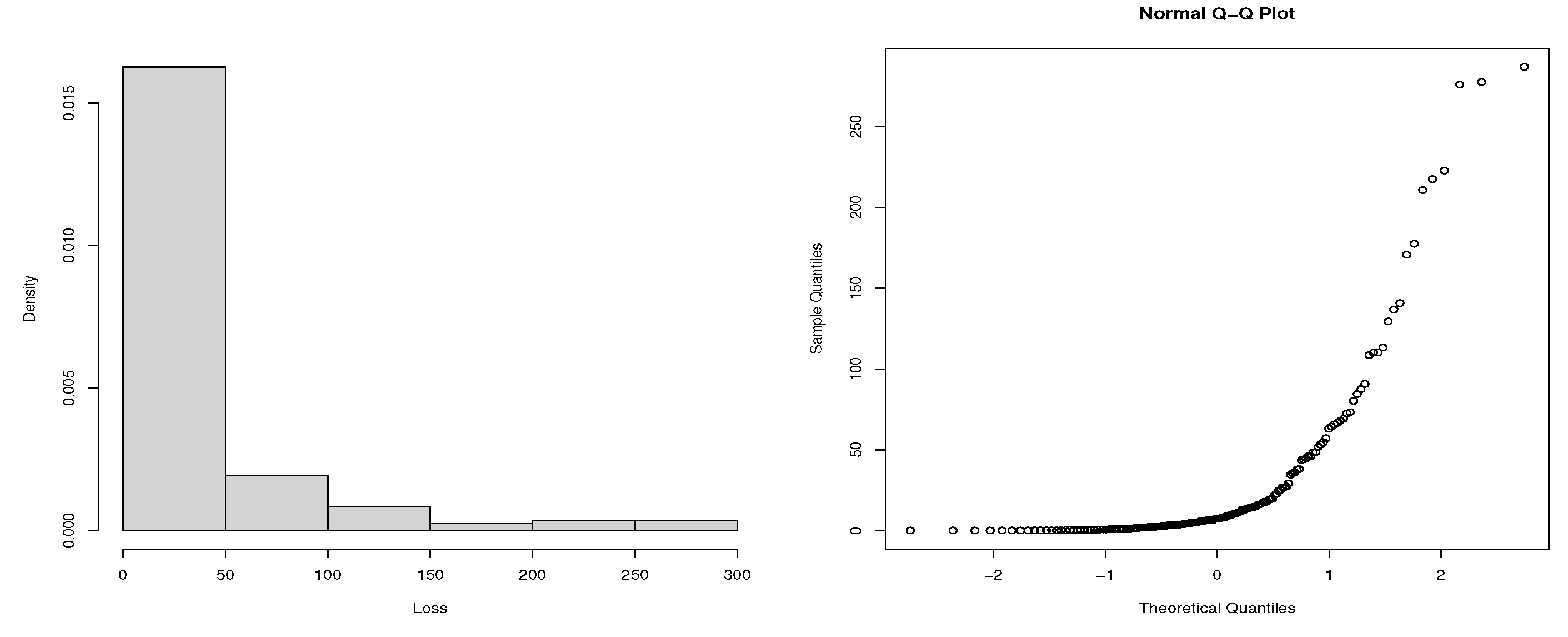
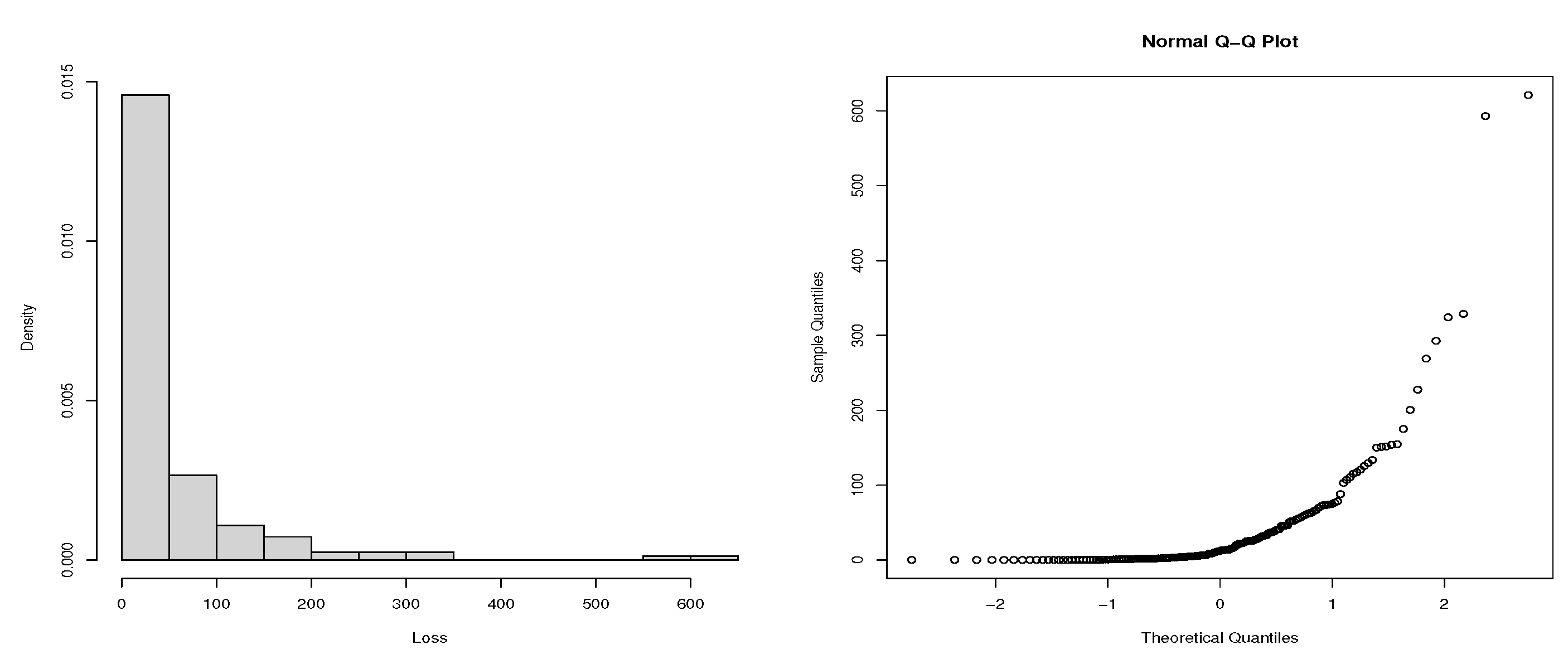
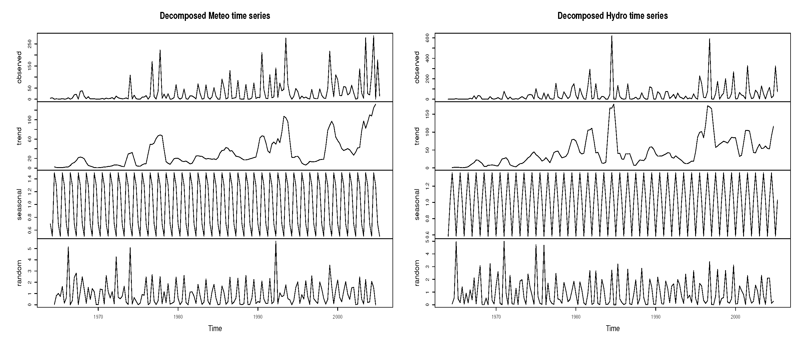
Table 1 presents summary statistics of losses due to the hydrological and meteorological disasters in Asia. The descriptive statistics together with the histogram and normal Q-Q plots (Figure 10 and Figure 11) suggest that the two datasets are both positively skewed and heavy-tailed. To isolate the deterministic components, the quarterly time series are decomposed under the multiplicative model assumption. Figure 12 presents the datasets decomposition which shows the presence of strong seasonal components in both variables and some evidence of weak long-term trends. Since the proposed model does not assume any deterministic seasonality, we deseasonalize by dividing each time series with its estimated seasonal component.

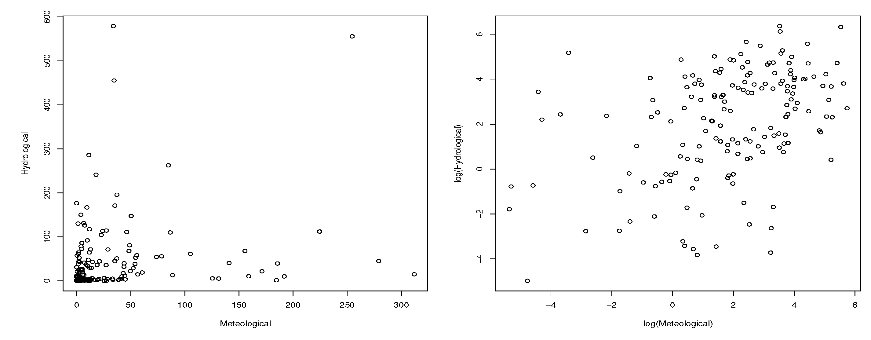
Figure 13 gives the scatter plots of the two deseasonalized variables and their log-transformed versions. The figure shows some evidence of a dependent relationship between the two variables. The sample Spearman’s rho and Kendall’s tau are 0.425 and 0.291, respectively.

We apply the EM algorithm described in Section 4.2 to fit the data using six specific bivariate models: GCR-GG, GCR-t, GCR-LG, GCR2-GG, GCR2-t, and GCR2-LG. For each model fitting, the EM algorithm requires the initialization of the parameter values. To obtain a reliable result, we first fit the marginal models separately using the estimation method given in [12], and the fitted values of the marginal parameters, i.e.,

(α_{i}, β_{i}, τ_{i}, θ)

for GCR models and

(α_{i}, β_{i}, τ_{i}, θ), i = 1, 2

, for the GCR2 models, are used for the initialization of the BVGCR (or BVGCR2) model parameters. For the mixture weight parameter initialization, we use a large set of possible parameter values satisfying

p_{11} + p_{12} = p_{1}

and

p_{11} + p_{21} = p_{2}

, where

p_{1}

and

p_{2}

are the mixture weight parameter estimates for the marginal models. The log-likelihood function values of the EM fits under the set of initializations are compared and the one gives the largest log-likelihood value is selected for the final fit.

Since the number of estimated model parameters differs by model, we compare the fits of candidate BVGCR2 models in terms of the Akaike information criterion (AIC) and the Bayesian information criterion (BIC), defined as

\begin{matrix} A I C & = & - 2 (Log - Likelihood) + 2 k \\ B I C & = & - 2 (Log - Likelihood) + k log n, \end{matrix}

respectively, where k is the number of estimated parameters and n is the sample size. Amongst candidate models, the preferred model is the one with the smallest value of either of these criteria. From Table 2, we see that the fitted BVGCR2-GG model outperforms all the other alternative models based on the Akaike information criterion. However, the BVGCR-LG model is preferred in terms of the Bayesian information criterion which heavily penalizes complex models. Comparing the BVGCR-GG to the BVGCR2-GG, one can see the BVGCR2-GG significantly improves model fitting due to the additional shape parameter.

Table 3 gives parameter estimates of the marginal distributions and the bivariate model of the fitted GCR2-GG model.

Note that the values of

(p_{11} + p_{12})

and

(p_{11} + p_{21})

based on the fitted BVGCR2-GG model are larger than the corresponding estimates of

p_{1}

and

p_{2}

. Spearman’s rho and Kendall’s tau under the fitted BVGCR2-GG model are 0.173 and 0.115, respectively, which are lower than the empirical counterparts. This may be because the empirical data contains spurious dependence due to the deterministic trend.

To test the statistical significance of the parameter estimates of the BVGCR2-GG model, we construct the bootstrap confidence intervals by computing the 2.5th and the 97.5th percentiles of the estimates based on the 100 bootstrap samples. Table 4 shows that all the parameter estimates on the original dataset fall in the corresponding 95% bootstrap confidence intervals.

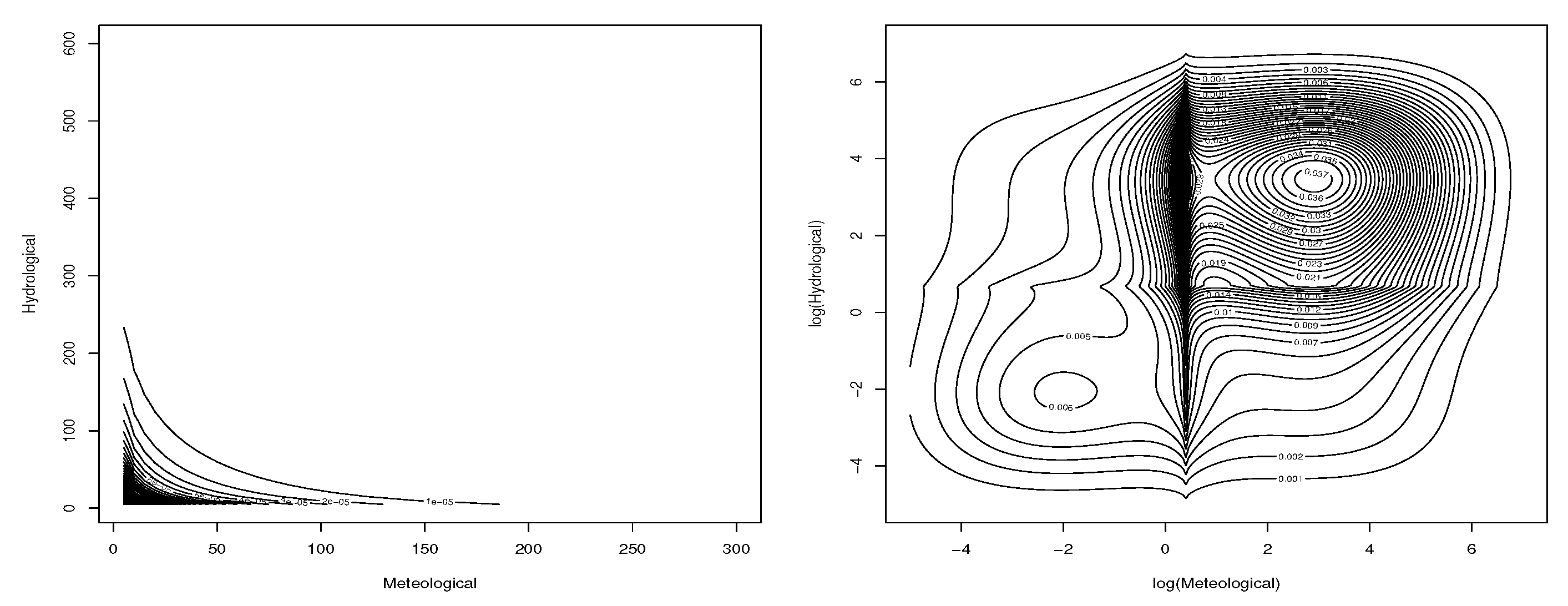
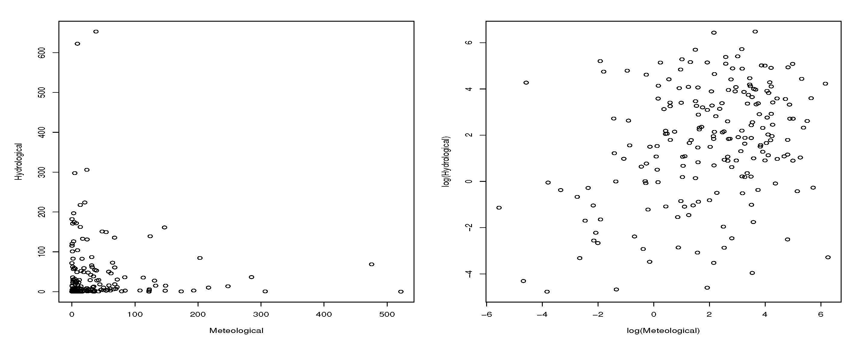
Figure 14 gives the contour plots of the fitted BVGCR2-GG model and that of the log-transformed random variables and Figure 15 presents the scatter plots of the simulated random variables from the BVGCR2-GG model and their log-transformations. Comparing these plots with Figure 13, we can see that the fitted model explains the dependence structure of the empirical data well.

6. Conclusions

In this paper, we constructed a bivariate extension of the Type-II generalized crack distribution and studied a few specific examples of the bivariate GCR2 distributions base on the generalized Gaussian, Student’s t and logistic densities to demonstrate the applicability of the constructed model. Specifically, our main theoretical finding is that the level of dependence of the constructed BVGCR2 model in terms of Kendall’s tau and Spearman’s rho is a weak to medium association. The model fitting to a catastrophic loss data showed that the fitted BVGCR2-GG model outperformed all the other alternative models based on the Akaike information criterion. Especially when compared to the BVGCR-GG model, the BVGCR2-GG model has shown a significant improvement due to the increased flexibility. With an appropriate choice of base density function, the propose BVGCR2 model can be effectively used for various applications that requires a weak to moderate level of dependence.

Author Contributions

Conceptualization, T. Bae; methodology, T.B., H.Q.; software, H.Q.; validation, T.B.; formal analysis, T.B, H.Q.; investigation, T.B.; resources, T.B.; data curation, H.Q.; writing—original draft preparation, T.B., H.Q.; writing—review and editing, T.B.; visualization, H.Q.; supervision, T.B.; project administration, T.B.; funding acquisition, T.B. All authors have read and agreed to the published version of the manuscript.

Funding

This research is supported by the Discovery Grant program of the Natural Science and Engineering Research Council of Canada (NSERC) with a funding reference number RGPIN-2022-03428

Data Availability Statement

The data used in this research is available upon request.

Conflicts of Interest

The authors declare no conflicts of interest.

Appendix A. Proof of Proposition 1

We drop parameters in the expressions of the functions for notational convenience and write

\bar{G} (\cdot) = 1 - G (\cdot)

and

b (t_{i}) = α_{i}^{- 1} [{(β_{i} / t_{i})}^{τ} - {(t_{i} / β_{i})}^{τ}], i = 1, 2 .

f_{B V G C R 2} (t_{1}, t_{2}; α, β, τ, p)

the joint distribution of

(T_{1}, T_{2})

having BVGCR2(

α

β

τ

,p;g), is

\begin{matrix} F (t_{1}, t_{2}) & = p_{11} F_{G C R 2}^{(1)} (t_{1}) F_{G C R 2}^{(1)} (t_{2}) + p_{12} F_{G C R 2}^{(1)} (t_{1}) F_{G C R 2}^{(2)} (t_{2}) \\ + p_{21} F_{G C R 2}^{(2)} (t_{1}) F_{G C R 2}^{(1)} (t_{2}) + p_{22} F_{G C R 2}^{(2)} (t_{1}) F_{G C R 2}^{(2)} (t_{2}), \end{matrix}

and the marginal density of

T_{i}, i = 1, 2,

f_{T_{i}} (t_{i}) = p_{i} f_{G C R 2}^{(1)} (t_{i}) + q_{i} f_{G C R 2}^{(2)} (t_{i}),

also, the cdf of GCR2

(t; α, β, τ, p)

distribution can be written as

F_{G C R 2} (t; α, β, τ, p) = 1 - G (b (t)) + (2 p - 1) H (t; α, β, τ, p),

where

p_{1} = p_{11} + p_{12}, p_{2} = p_{11} + p_{21}, q_{i} = 1 - p_{i}, i = 1, 2

G (x) = \int_{- \infty}^{x} g (s) d s

is the cdf of g and

H (t; α, β, τ, p) = \int_{b (t)}^{\infty} \frac{s}{\sqrt{s^{2} + 4 / α^{2}}} g (s) d s .

By expanding the integrand in Equation 6 using these expressions and taking the double integration, we have

\begin{matrix} \int_{0}^{\infty} \int_{0}^{\infty} F (t_{1}, t_{2}) f_{T_{1}} (t_{1}) f_{T_{2}} (t_{2}) d t_{1} d t_{2} \\ = p_{11} {p_{1} p_{2} E [F_{S_{1}} (S_{1})] E [F_{S_{2}} (S_{2})] + p_{1} q_{2} ζ_{2} E [F_{S_{1}} (S_{1})] + q_{1} p_{2} ζ_{1} E [F_{S_{2}} (S_{2})] + q_{1} q_{2} ζ_{1} ζ_{2}} \\ + p_{12} {p_{1} p_{2} η_{2} E [F_{S_{1}} (S_{1})] + p_{1} q_{2} E [F_{S_{1}} (S_{1})] E [F_{V_{2}} (V_{2})] + q_{1} p_{2} ζ_{1} η_{2} + q_{1} q_{2} ζ_{1} E [F_{V_{2}} (V_{2})]} \\ + p_{21} {p_{1} p_{2} η_{1} E [F_{S_{2}} (S_{2})] + p_{1} q_{2} η_{1} ζ_{2} + q_{1} p_{2} E [F_{V_{1}} (V_{1})] E [F_{S_{2}} (S_{2})] + q_{1} q_{2} ζ_{2} E [F_{V_{2}} (V_{2})]} \\ + p_{22} {p_{1} p_{2} η_{1} η_{2} + p_{1} q_{2} η_{1} E [F_{V_{2}} (V_{2})] + q_{1} p_{2} η_{2} E [F_{V_{1}} (V_{1})] + q_{1} q_{2} E [F_{V_{1}} (V_{1})] E [F_{V_{2}} (V_{2})]} . \end{matrix}

where, for each

i = 1, 2,

\begin{matrix} E [F_{S_{i}} (S_{i})] = \int_{0}^{\infty} F_{G C R 2}^{(1)} (t_{i}) f_{G C R 2}^{(1)} (t_{i}) d t_{i} = \frac{1}{2} \\ E [F_{V_{i}} (V_{i})] = \int_{0}^{\infty} F_{G C R 2}^{(2)} (t_{i}) f_{G C R 2}^{(2)} (t_{i}) d t_{i} = \frac{1}{2} \\ ζ_{i} & : = \int_{0}^{\infty} F_{G C R 2}^{(1)} (t_{i}) f_{G C R 2}^{(2)} (t_{i}) d t_{i} \\ = \int_{0}^{\infty} [F_{G C R 2}^{(2)} (t_{i}) + 2 H (t_{i})] f_{G C R 2}^{(2)} (t_{i}) d t_{i} \\ = E [F_{V_{i}} (V_{i})] + 2 \int_{0}^{\infty} [H (t_{i}) f_{G C R 2}^{(2)} (t_{i})] d t_{i} = \frac{1}{2} + 2 \int_{0}^{\infty} [H (t_{i}) f_{G C R 2}^{(2)} (t_{i})] d t_{i} \\ η_{i} & : = \int_{0}^{\infty} F_{G C R 2}^{(2)} (t_{i}) f_{G C R 2}^{(1)} (t_{i}) d t_{i} \\ = \int_{0}^{\infty} [F_{G C R 2}^{(1)} (t_{i}) + 2 H (t_{i})] f_{G C R 2}^{(1)} (t_{i}) d t_{i} \\ = E [F_{S_{i}} (S_{i})] - 2 \int_{0}^{\infty} [H (t_{i}) f_{G C R 2}^{(1)} (t_{i})] d t_{i} = \frac{1}{2} - 2 \int_{0}^{\infty} [H (t_{i}) f_{G C R 2}^{(1)} (t_{i})] d t_{i} . \end{matrix}

That is, the evaluating the double integral in Equation 6 reduces to the following two integrals:

\int_{0}^{\infty} H (t) f_{G C R 2}^{(1)} (t) d t

and

\int_{0}^{\infty} H (t) f_{G C R 2}^{(2)} (t) d t

. Due to the expression

F_{G C R 2}^{(1)} (t) = 1 - G (b (t)) + H (t)

and

\begin{matrix} \int_{- \infty}^{\infty} H (b^{- 1} (s)) \frac{s}{\sqrt{s^{2} + 4 / α^{2}}} g (s) d s \\ = \int_{- \infty}^{\infty} (\int_{s}^{\infty} \frac{z}{\sqrt{z^{2} + 4 / α^{2}}}) \frac{s}{\sqrt{s^{2} + 4 / α^{2}}} g (s) d s = 0, \end{matrix}

and changing the order of integrations, we obtain

\begin{matrix} \int_{0}^{\infty} H (t) f_{G C R 2}^{(1)} (t) d t & = \int_{0}^{\infty} \int_{b (t)}^{\infty} \frac{s}{\sqrt{s^{2} + 4 / α^{2}}} g (s) d s f_{G C R 2}^{(1)} (t) d t \\ = \int_{- \infty}^{\infty} (\int_{b^{- 1} (s)}^{\infty} f_{G C R 2}^{(1)} (t) d t) \frac{s}{\sqrt{s^{2} + 4 / α^{2}}} g (s) d s \\ = \int_{- \infty}^{\infty} (1 - F_{G C R 2}^{(1)} (b^{- 1} (s))) \frac{s}{\sqrt{s^{2} + 4 / α^{2}}} g (s) d s \\ = \int_{- \infty}^{\infty} (G (s) - H (b^{- 1} (s))) \frac{s}{\sqrt{s^{2} + 4 / α^{2}}} g (s) d s \\ = \int_{- \infty}^{\infty} G (s) \frac{s}{\sqrt{s^{2} + 4 / α^{2}}} g (s) d s - \int_{- \infty}^{\infty} H (b^{- 1} (s)) \frac{s}{\sqrt{s^{2} + 4 / α^{2}}} g (s) d s \\ = \int_{- \infty}^{\infty} \frac{s}{\sqrt{s^{2} + 4 / α^{2}}} G (s) g (s) d s = γ . \end{matrix}

Similarly, due to the expression

F_{G C R 2}^{(2)} (t) = 1 - G (b (t)) - H (t)

, we obtain

\begin{matrix} \int_{0}^{\infty} H (t) f_{G C R 2}^{(2)} (t) d t & = \int_{0}^{\infty} \int_{b (t)}^{\infty} \frac{s}{\sqrt{s^{2} + 4 / α^{2}}} g (s) d s f_{G C R 2}^{(2)} (t) d t \\ = \int_{- \infty}^{\infty} (\int_{b^{- 1} (s)}^{\infty} f_{G C R 2}^{(2)} (t) d t) \frac{s}{\sqrt{s^{2} + 4 / α^{2}}} g (s) d s \\ = \int_{- \infty}^{\infty} (1 - F_{G C R 2}^{(2)} (b^{- 1} (s))) \frac{s}{\sqrt{s^{2} + 4 / α^{2}}} g (s) d s \\ = \int_{- \infty}^{\infty} (G (s) + H (b^{- 1} (s))) \frac{s}{\sqrt{s^{2} + 4 / α^{2}}} g (s) d s \\ = \int_{- \infty}^{\infty} G (s) \frac{s}{\sqrt{s^{2} + 4 / α^{2}}} g (s) d s + \int_{- \infty}^{\infty} H (b^{- 1} (s)) \frac{s}{\sqrt{s^{2} + 4 / α^{2}}} g (s) d s \\ = \int_{- \infty}^{\infty} \frac{s}{\sqrt{s^{2} + 4 / α^{2}}} G (s) g (s) d s = γ . \end{matrix}

The combination and some simplifications of these results give the expression Equation 7.

Appendix B. Proof of Proposition 2

As in the proof of proposition 1, expanding the integrand in 8 using the joint cdf and pdf of the BVGCR2 and taking double integrals, gives

\begin{matrix} \int_{0}^{\infty} \int_{0}^{\infty} F (t_{1}, t_{2}) f (t_{1}, t_{2}) d t_{1} d t_{2} \\ = {(p_{11})}^{2} E [F_{S_{1}} (S_{1})] E [F_{S_{2}} (S_{2})] + p_{11} p_{12} ζ_{2} E [F_{S_{1}} (S_{1})] + p_{11} p_{21} ζ_{1} E [F_{S_{2}} (S_{2})] \\ + p_{11} p_{22} ζ_{1} ζ_{2} + p_{12} p_{11} η_{2} E [F_{S_{1}} (S_{1})] + {(p_{12})}^{2} E [F_{S_{1}} (S_{1})] E [F_{V_{2}} (V_{2})] \\ + p_{12} p_{21} ζ_{1} η_{2} + p_{12} p_{22} ζ_{1} E [F_{V_{2}} (V_{2})] + p_{21} p_{11} η_{1} E [F_{S_{2}} (S_{2})] + p_{21} p_{12} η_{1} ζ_{2} \\ + {(p_{21})}^{2} E [F_{V_{1}} (V_{1})] E [F_{S_{2}} (S_{2})] + p_{21} p_{22} ζ_{2} E [F_{V_{2}} (V_{2})] + p_{22} p_{11} η_{1} η_{2} \\ + p_{21} p_{11} η_{1} E [F_{V_{2}} (V_{2})] + p_{22} p_{21} η_{2} E [F_{V_{1}} (V_{1})] + {(p_{22})}^{2} E [F_{V_{1}} (V_{1})] E [F_{V_{2}} (V_{2})] . \end{matrix}

As given the proof of Proposition 1,

E [F_{S_{1}} (S_{1})] = E [F_{V_{2}} (V_{2})] = \frac{1}{2}, ζ_{i} = \frac{1}{2} + 2 γ_{i}

and

η_{i} = \frac{1}{2} - 2 γ_{i}

for each

i = 1, 2

. With these and after some simplification, the above integral can be expressed as

\int_{0}^{\infty} \int_{0}^{\infty} F (t_{1}, t_{2}) f (t_{1}, t_{2}) d t_{1} d t_{2} = \frac{1}{4} + 8 (p_{11} p_{22} - p_{12} p_{21}) γ_{1} γ_{2} .

Appendix C. Proof of Lemma 4.1

The log-likelihood function of the observed data is given as

l (θ) = log p (\underset{˜}{x} | θ)

. By the law of total probability,

log p (\underset{˜}{x} | θ) = log \sum_{\underset{˜}{z}} p (\underset{˜}{x} | \underset{˜}{z}, θ) p (\underset{˜}{z} | θ) = log \sum_{\underset{˜}{z}} p (\underset{˜}{x}, \underset{˜}{z} | θ) .

Multiplying and dividing by a constant

p (\underset{˜}{z} | \underset{˜}{x}, θ^{(m)})

, which is the probability of hidden data given the observed data and initial guess parameter. Since this is a probability function, then

p (\underset{˜}{z} | \underset{˜}{x}, θ^{(m)}) \geq 0

and

\sum_{\underset{˜}{z}} p (\underset{˜}{z} | \underset{˜}{x}, θ^{(m)}) = 1

. Then, the log-likelihood is;

\begin{matrix} l (θ) & = & log \sum_{\underset{˜}{z}} p (\underset{˜}{z} | \underset{˜}{x}, θ^{(m)}) \frac{p (\underset{˜}{x}, \underset{˜}{z} | θ)}{p (\underset{˜}{z} | \underset{˜}{x}, θ^{(m)})}, \\ = & log E_{Z | \underset{˜}{x}, θ^{(m)}} [\frac{p (\underset{˜}{x}, Z | θ)}{p (Z | \underset{˜}{x}, θ^{(m)})}], \\ \geq & E_{Z | \underset{˜}{x}, θ^{(m)}} [log \frac{p (\underset{˜}{x}, Z | θ)}{p (Z | \underset{˜}{x}, θ^{(m)})}] b y J e n s e n i n e q u a l i t y, \\ = & E_{Z | \underset{˜}{x}, θ^{(m)}} [log p (\underset{˜}{x}, Z | θ)] - E_{Z | \underset{˜}{x}, θ^{(m)}} [log p (Z | \underset{˜}{x}, θ^{(m)})], \\ = & Q (θ | θ^{(m)}) - E_{Z | \underset{˜}{x}, θ^{(m)}} [log p (Z | \underset{˜}{x}, θ^{(m)})], \\ l (θ) & \geq & Q (θ | θ^{(m)}) - h (θ^{(m)}) . \end{matrix}

Therefore,

Q (θ | θ^{(m)})

gives the lower bound on the log-likelihood, which is the only term that depends on

θ

l (θ) \geq Q (θ | θ^{(m)}) - h (θ^{(m)})

is true for all

θ

including the situation where

θ = θ^{(m)}

. We show the relationship is still true for

θ = θ^{(m)}

\begin{matrix} \sum_{\underset{˜}{z}} p (\underset{˜}{z} | \underset{˜}{x}, θ^{(m)}) l o g \frac{p (\underset{˜}{x}, \underset{˜}{z} | θ^{(m)})}{p (\underset{˜}{z} | \underset{˜}{x}, θ^{(m)})}, \\ = & \sum_{\underset{˜}{z}} p (\underset{˜}{z} | \underset{˜}{x}, θ^{(m)}) l o g p (\underset{˜}{x} | θ^{(m)}) b y B a y e s^{'} t h e o r e m, \\ = & log p (\underset{˜}{x} | θ^{(m)}) \sum_{\underset{˜}{z}} p (\underset{˜}{z} | \underset{˜}{x}, θ^{(m)}) = : l (θ^{(m)}) . \end{matrix}

If we have

θ

for which

Q (θ | θ^{(m)}) \geq Q (θ^{(m)} | θ^{(m)})

, then

l (θ) + h (θ^{(m)}) \geq Q (θ | θ^{(m)}) \geq Q (θ^{(m)} | θ^{(m)}) = l (θ^{(m)}) + h (θ^{(m)}) .

Therefore, as Q increases, it implies

log p (\underset{˜}{x} | θ)

also increases. We conclude that, if

θ

is the MLE, then

l (θ) \geq l (θ^{(m + 1)}) \geq l (θ^{(m)}),

always holds.

References

Bingham, N.H.; Goldie, C.M.; Teugels, J.L. Regular Variation; Cambridge University Press, 1987.
Embrechts, P.; Klüppelberg, C.; Mikosch, T. Modelling Extremal Events for Insurance and Finance; Springer-Verlag: Berlin, 1997. [Google Scholar]
Foss, S.; Korshunov, D.; Zachary, S. An Introduction to Heavy-Tailed and Subexponential Distributions; Springer Science+Business Media, 2013.
Birnbaum, Z.W.; Saunders, S.C. A new family of life distributions. Journal of applied probability 1969, 6, 319–327. [Google Scholar] [CrossRef]
Leiva, V. The Birnbaum-Saunders Distribution 2015.
Díaz-García, J.A.; Leiva-Sánchez, V. A new family of life distributions based on the elliptically contoured distributions. Journal of Statistical Planning and Inference 2005, 128, 445–457. [Google Scholar] [CrossRef]
Gomes, M.I.; Ferreira, M.; Leiva, V. The extreme value Birnbaum-Saunders model, its moments and an application in biometry. Biometrical Letters 2012, 49, 81–94. [Google Scholar] [CrossRef]
Ferreira, M.; Gomes, M.I.; Leiva, V. On an extreme value version of the Birnbaum–Saunders distribution. REVSTAT-Statistical Journal 2012, 10, 181–210. [Google Scholar]
Volodin, I.N.; Dzhungurova, O.A. On limit distributions emerging in the generalized Birnbaum-Saunders model. Journal of Mathematical Sciences 2000, 99, 1348–1366. [Google Scholar] [CrossRef]
Bae, T.; Chen, J. On heavy-tailed crack distribution for loss severity modeling. International Journal of Statistics and Probability 2017, 6, 92–110. [Google Scholar] [CrossRef]
Mazjini, M.; Bae, T. Statistical modelling of precipitation data in Canadian Prairies with a dynamic mixture structure. Theoretical and Applied Climatology 2023, 153, 173–192. [Google Scholar] [CrossRef]
Bae, T.; Volodin, A. Type-II Generalized Crack Distribution with Application to Heavy-Tailed Data Modeling. Journal of Statistical Theory and Practice 2022, 16, 1–23. [Google Scholar] [CrossRef]
Bae, T.; Choi, Y.H. A bivariate extension of three-parameter generalized crack distribution for loss severity modelling. Journal of the Korean Statistical Society 2022, 51, 378–402. [Google Scholar] [CrossRef]
Klugman, S.A.; Panjer, H.H.; Willmot, G.E. Loss models: from data to decisions; Vol. 715, John Wiley & Sons, 2012.
Dempster, A.P.; Laird, N.M.; Rubin, D.B. Maximum likelihood from incomplete data via the EM algorithm. Journal of the royal statistical society: series B (methodological) 1977, 39, 1–22. [Google Scholar] [CrossRef]

Figure 1. Density functions of GCR2-t distribution with

α

= 0.5,

β

= 5 ,

τ

\in {0.3, 0.5, 0.8}

, p = 0.5, and

ν

= 3.

Figure 1. Density functions of GCR2-t distribution with

α

= 0.5,

β

= 5 ,

τ

\in {0.3, 0.5, 0.8}

, p = 0.5, and

ν

= 3.

Figure 2. Density functions of GCR2-t distribution with

α

\in {0.25, 0.75, 1}

β

= 5 ,

τ = 0.3

, p = 0.5, and

ν

= 5.

Figure 2. Density functions of GCR2-t distribution with

α

\in {0.25, 0.75, 1}

β

= 5 ,

τ = 0.3

, p = 0.5, and

ν

= 5.

Figure 3. Density functions of GCR2-t distribution with

α

= 0.75,

β

= 5 ,

τ

= 0.5, p

\in {0.3, 0.5, 0.8}

and

ν

= 5.

Figure 3. Density functions of GCR2-t distribution with

α

= 0.75,

β

= 5 ,

τ

= 0.5, p

\in {0.3, 0.5, 0.8}

and

ν

= 5.

Figure 4. Density functions of GCR2-GG distribution with

α = 0.75

β

= 5 ,

τ

\in {0.3, 0.5, 0.8}

, p = 0.5, and

θ

= 0.8.

Figure 4. Density functions of GCR2-GG distribution with

α = 0.75

β

= 5 ,

τ

\in {0.3, 0.5, 0.8}

, p = 0.5, and

θ

= 0.8.

Figure 5. Density functions of GCR2-GG distribution with

α = 1

β

= 5 ,

τ = 0.5

, p

\in {0.2, 0.5, 0.8}

, and

θ

= 1.

Figure 5. Density functions of GCR2-GG distribution with

α = 1

β

= 5 ,

τ = 0.5

, p

\in {0.2, 0.5, 0.8}

, and

θ

= 1.

Figure 6. Density functions of GCR2-GG distribution with

α

\in {0.5, 0.75, 1}

β

= 5 ,

τ = 0.5

, p = 0.5, and

θ

= 1.2.

Figure 6. Density functions of GCR2-GG distribution with

α

\in {0.5, 0.75, 1}

β

= 5 ,

τ = 0.5

, p = 0.5, and

θ

= 1.2.

Figure 7. Density functions of GCR2-LG distribution with

α

= 1,

β

= 5 ,

τ = 0.5

and p

\in {0.2, 0.5, 0.8}

Figure 7. Density functions of GCR2-LG distribution with

α

= 1,

β

= 5 ,

τ = 0.5

and p

\in {0.2, 0.5, 0.8}

Figure 8. Density functions of GCR2-LG distribution with

α

=0.75 ,

β

= 5 ,

τ

\in {0.5, 0.75, 1}

and p = 0.5.

Figure 8. Density functions of GCR2-LG distribution with

α

=0.75 ,

β

= 5 ,

τ

\in {0.5, 0.75, 1}

and p = 0.5.

Figure 9. Density functions of GCR2-LG distribution with

α

\in {0.5, 0.75, 0.9}

β

= 5 ,

τ = 0.3

and p = 0.5.

Figure 9. Density functions of GCR2-LG distribution with

α

\in {0.5, 0.75, 0.9}

β

= 5 ,

τ = 0.3

and p = 0.5.

Figure 10. Histogram of Meteo loss dataset and its normal Q-Q plot.

Figure 11. Histogram of Hydro loss dataset and its normal Q-Q plot.

Figure 12. Multiplicative decompositions of Meteo and Hydro time series.

Figure 13. Scatter plots of the deseasonalized data and their log-transformations.

Figure 14. Contour plots of the fitted BVGCR2-GG density and the density of the log-transformed random variables.

Figure 15. Scatter plots of simulated random variables from the fitted BVGCR2-GG model and their log-transformations.

Table 1. Descriptive summary statistics of the dataset (Unit: 100 million USD).

Data	n	Min	1st Qu.	Median	Mean	3rd Qu.	Max	Skewness	Kurtosis
Meteo	166	0.003	2.005	7.275	30.799	35.282	287.090	2.820	11.304
Hydro	166	0.007	1.692	12.172	45.538	53.330	621.207	4.014	23.188

Table 2. Model comparison with AIC and BIC.

Model	Log-likelihood	AIC	BIC
BVGCR-GG	-1370.332	2758.664	2786.672
BVGCR-t	-1372.381	2762.762	2790.770
BVGCR-LG	-1372.066	2758.132	2779.916
BVGCR2-GG	-1367.346	2756.692	2790.924
BVGCR2-t	-1371.782	2765.564	2799.796
BVGCR2-LG	-1371.707	2761.414	2789.422

Table 3. Parameter estimates of marginals and Bivariate GCR2-GG models.

	${\hat{α}}_{1}$	${\hat{β}}_{1}$	${\hat{τ}}_{1}$	${\hat{θ}}_{1}$	$\hat{p_{1}}$	${\hat{α}}_{2}$	${\hat{β}}_{2}$	${\hat{τ}}_{2}$	${\hat{θ}}_{2}$	$\hat{p_{2}}$	${\hat{p}}_{11}$	${\hat{p}}_{12}$	${\hat{p}}_{21}$	${\hat{p}}_{22}$
Meteo	20.075	0.915	0.737	0.623	0.094
Hydro						11.152	1.964	0.669	0.809	0.189
Bivariate	22.644	1.494	0.791	0.477		11.442	1.964	0.675	0.798		0.124	0.040	0.072	0.764

Table 4. The 95% bootstrap confidence intervals for the parameters in Bivariate GCR2-GG model

	${\hat{α}}_{1}$	${\hat{β}}_{1}$	${\hat{τ}}_{1}$	${\hat{θ}}_{1}$	${\hat{α}}_{2}$	${\hat{β}}_{2}$	${\hat{τ}}_{2}$	${\hat{θ}}_{2}$	${\hat{p}}_{11}$	${\hat{p}}_{12}$	${\hat{p}}_{21}$	${\hat{p}}_{22}$
Original estimate	22.644	1.494	0.791	0.477	11.442	1.964	0.675	0.798	0.124	0.040	0.072	0.764
Bootstrap mean	27.673	1.524	0.735	0.583	14.189	2.065	0.680	0.988	0.131	0.037	0.067	0.766
2.5th percentile	7.031	0.762	0.542	0.347	2.356	1.500	0.322	0.418	0.059	0.000	0.000	0.687
97.5th percentile	52.149	2.252	0.951	1.013	42.898	2.803	0.913	3.027	0.192	0.080	0.147	0.843

Disclaimer/Publisher’s Note: The statements, opinions and data contained in all publications are solely those of the individual author(s) and contributor(s) and not of MDPI and/or the editor(s). MDPI and/or the editor(s) disclaim responsibility for any injury to people or property resulting from any ideas, methods, instructions or products referred to in the content.

© 2024 by the authors. Licensee MDPI, Basel, Switzerland. This article is an open access article distributed under the terms and conditions of the Creative Commons Attribution (CC BY) license (http://creativecommons.org/licenses/by/4.0/).

Copyright: This open access article is published under a Creative Commons CC BY 4.0 license, which permit the free download, distribution, and reuse, provided that the author and preprint are cited in any reuse.

MDPI Initiatives

Important Links

Choose an area of interest and we will send you notifications of new preprints at your preferred frequency.

Disclaimer

A Bivariate Extension of Type II Generalized Crack Distribution for Modelling Heavy-Tailed Losses

Abstract

1. Introduction

2. Type-II Generalized Crack Distribution

2.1. Birnbaum-Saunders Distribution

2.2. Gaussian Crack (CR) Distribution

2.3. Generalized Crack Distribution

2.4. Type-II Birnbaum-Saunders (BS2) Distribution

2.5. Type-II Generalized Crack Distribution

2.6. Specific Examples of GCR2 Distributions

3. Bivaraite GCR2 Distribution

3.1. Dependence Measures

3.1.1. Spearman’s Rho

3.1.2. Kendall’s Tau

3.2. Tail Independence

4. Model Parameter Estimation

4.1. Maximum Likelihood Estimation

4.2. Expectation-Maximization Algorithm

5. Applications

6. Conclusions

Author Contributions

Funding

Data Availability Statement

Conflicts of Interest

Appendix A. Proof of Proposition 1

Appendix B. Proof of Proposition 2

Appendix C. Proof of Lemma 4.1

References

MDPI Initiatives

Important Links

Subscribe