1. Introduction
The horticultural greenhouse facility area in China is now 3.7 million hectares. Solar greenhouses are the major type in northern provinces due to their heat preservation and low energy cost [
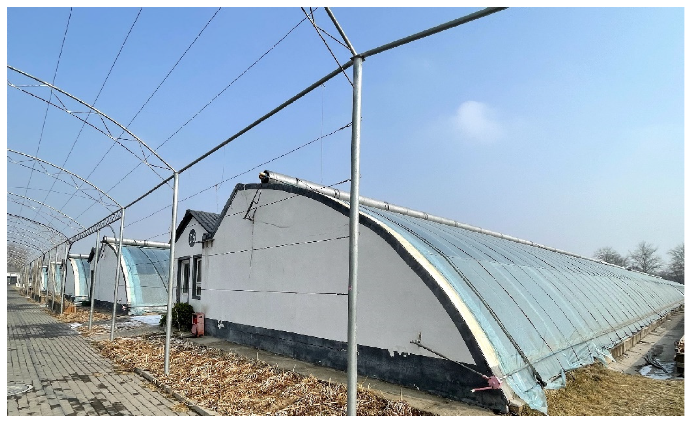
1]. In recent years, the agriculture production facilities progressively evolved towards greenhouse clusters which impact the ventilation of each greenhouse (
Figure 1). The spacing between each other is usually small, which makes it necessary to study the validity of most current two-dimensional CFD (Computational Fluid Dynamics) studies in this ubiquitous scenario. Up to now, most of the current CFD studies focus on a single greenhouse, especially for the typical Chinese solar greenhouse (CSG), the wind field and ventilation rate around and inside multiple greenhouses has not been fully studied [
2]. However, the real situation is that the model is usually used in greenhouse clusters, which causes differences compared with ideal experiments.
Estimation of ventilation rate is an indispensable part in modelling the greenhouse climate, as well as for controlling the climate inside the greenhouse, which is essential for cooling and dehumidification. Ventilation is achieved either by natural ventilation or by forced ventilation facilities (e.g. exhaust fan and fan-pad cooling system) [
3]. Natural ventilation is currently widely preferred by farmers in practical production, given its low energy cost [
4,
5,
6]. Natural ventilation is driven by two forces induced by wind and thermal gradients [
7,
8]. On contrary to mechanically forced ventilation, natural ventilation is characterized by varied input conditions and hence it makes it difficult to quantify the flow rate.
Gas tracing and energy balance are two common methods to obtain the ventilation rate before the CFD technique was adopted in the last two decades to simulate the greenhouse flow field [
9]. The gas tracing method requires that the tracer gas distribution be uniform inside the greenhouse before opening the vents and its concentration over a given operation point [
10]. The energy balance method relies greatly on the accuracy of the flux sensors or the greenhouse model [
11]. In addition to the inconvenient practice, both methods have an error of up to 30% [
12]. Compared with the above methods, the cost of the CFD method is lower, and in addition, this approach guarantees a high level of accuracy, provided that the quality of the mesh, the optimal design of the model in the flow field, and the convergence of the solution are correctly checked.
CFD technique has been widely applied in the optimal design and the simulation of ventilation since the 1990s [
7,
13]. In the 21
st century, more comprehensive models were developed including the interaction between the microclimate and the crop [
14,
15,
16,
17,
18,
19,
20]. By using the CFD method, the impact of wind speed, vent opening configuration, and greenhouse structures on the airflow pattern have been investigated by many researchers [
8,
21,
22]. Bournet and Boulard (2010) reviewed optimum solutions for designers and analyzed the effect of ventilator configurations on the distributed climate inside greenhouses from CFD simulations published over 25 years [
23].
Up until recently, a vast majority of current research focused on 2D models [
23,
24,
25]. Some of them being especially applied to CSG [
26,
27,
28,
29]. With the progress of the computing power, there are more and more available 3D studies [
28]. Improving the mesh quality of 3D mesh requires proficient skills of designers. For the CSG, the fan-shaped geometry of the south roof makes it a challenge to create boundary layer grids. In addition, the calculation load of three-dimensional CFD model is heavy. These are why two-dimensional models have been widely used. Moreover, the impact of the surrounding buildings on the wind velocity distribution, and on the greenhouse ventilation has been hardly considered in previous two-dimensional CFD models. It is known however that the ventilation rate of a greenhouse with restricted vents opening areas is proved to be greatly reduced when neighbouring objects are high enough to disturb the flow [
30]. In the present study, the impact of building obstacles in front and behind the greenhouse on the ventilation rate is studied separately using 2D and 3D modelling. 20 cases were selected (10 cases for 2D and 10 cases for 3D) to compare the corresponding predicted natural ventilation rate and the wind field with the aim to validate the model. In cases where 2D models have been proven to replace 3D models, fast two-dimensional CFD simulations can be obtained with a large sample size, in order to study the greenhouse natural ventilation.
Using CFD model to obtain ventilation rate requires complex steps such as geometric modeling, meshing, coding functions, and defining boundary conditions. It also relies on the modeler’s skill in mesh design, and problem understanding and formalizing. It usually requires mesh reconstruction and boundary condition redefining when vent configuration or building structures are different, which necessitate relatively heavy workloads and hence makes it primarily implemented for research purposes rather than for practical use [
31]. From enough CFD samples, it could be possible to develop a black box model for natural ventilation. Indeed, conducting virtual wind tunnel simulations to obtain comprehensive and orderly samples is feasible, whereas it would be difficult to obtain a sufficient number of samples in field experiments, due to unstable and unpredictable weather conditions [
32]. In this study, from a high number of CFD simulations (990 cases), a natural ventilation rate model was developed using a nonlinear regression tree-model [
33]. As a result, by combining CFD simulations and tree-models, it is possible to assess the ventilation characteristics, making it possible to avoid identifying several parameters that are difficult to measure (e.g. wind pressure, thermal pressure), which is a significant step forward for optimal design or real-time greenhouse climate simulation.
2. Materials and Methods
2.1. Experimental Greenhouses and Vent Configurations
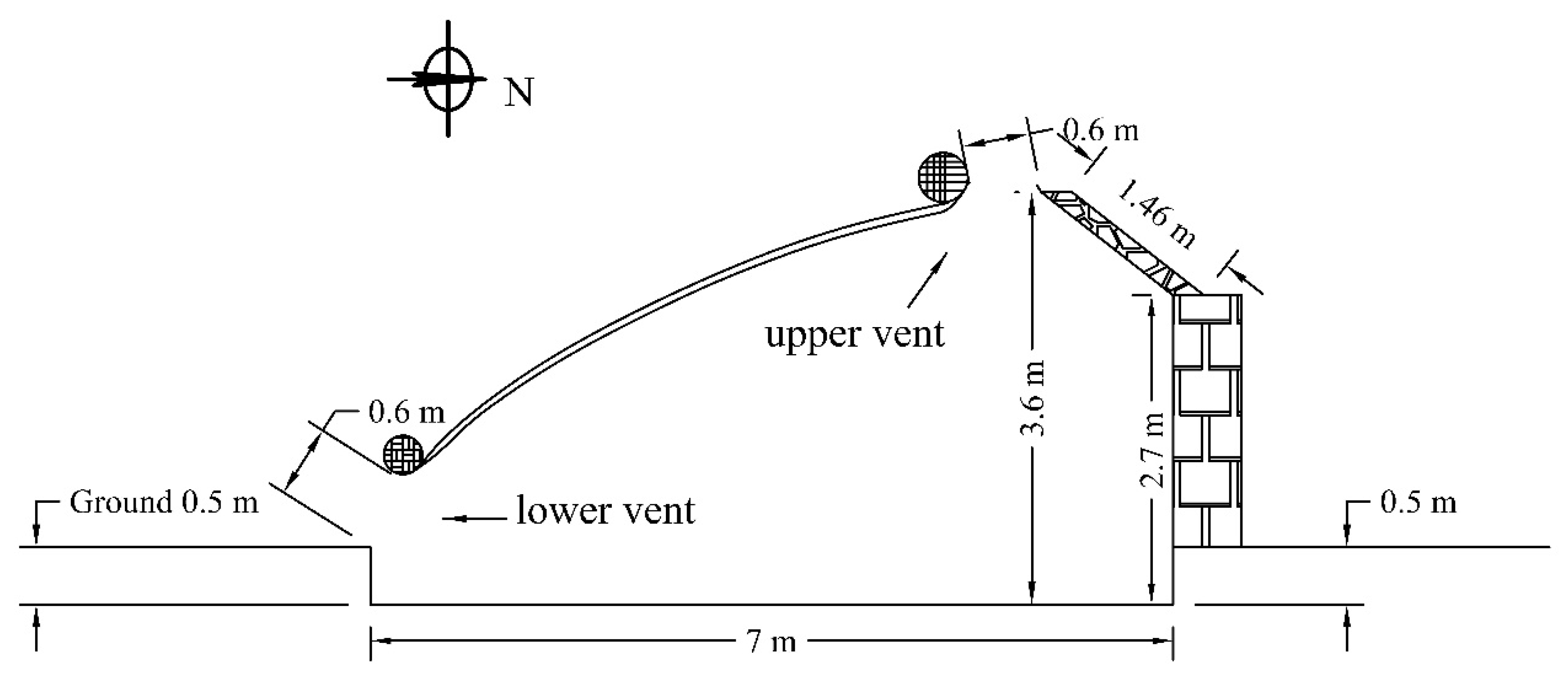
The object considered for the present study is the typical single slope solar greenhouse in China (
Figure 2). These greenhouses are distributed in rows along the west-east direction. The roof vent (upper vent) and side vent (lower vent) are both equipped with a rolling film. The width of the full vent opening for both the upper and the lower vent is 0.6 m. The ventilation rates for 9 different vent configurations were assessed in the experiment (
Table 1). Crops were not considered in this experiment, because the aim of this study is to obtain a general ventilation rate model that is applied to most of the CSGs, and the specific crop height or leaf area index could affect the ventilation rate and thus limit the application scope.
2.2. Calculation Domain
The CFD mesh was generated based on a 1:1 scale greenhouse i.e. considering the actual size of the greenhouse. For the study, 3 greenhouses were meshed in the flow field, with an interval of 4 m, and in addition, 9 different vent combinations of the upper vent and the lower vent were designed as described in
Table 1, considering the same combination for all three greenhouses. The height of the calculation domain is 14 m and the length of the upstream portion is determined as 3 times the ridge height (10.8 m), while the downstream portion is 10 times the ridge height (36 m,
Figure 3). Indeed, it was established that the backflow cannot form inside the computational domain within 10 times of the ridge height [
34]. Based on the same size as the above 2D domain, the 3D domain includes three greenhouses with a width of 50 m and an extension of 86 m on both sides of the greenhouses.
2.3. Models, Solver, and Material
The Reynolds-Averaged Navier-Stokes equations for mass, momentum, energy, and standard k-ε viscous model combined with buoyancy effect (g= -9.81 m s
-2) were solved by the SIMPLEC (Semi-Implicit for Pressure Linked Equations Consistent) method using Fluent
TM software [
35]. The flow in the near-wall region was solved using the Standard Wall Function. The incompressible-ideal-gas was used as state law to link the temperature and pressure. The corresponding physical properties of air specified in the model are gathered in
Table 2.
2.4. Generation of the Mesh File
The mesh file was generated by ICEM software (Ansys Inc., PA, USA). The blocks were associated with a set of grids, which were then converted to unstructured grids when generating the mesh file. The height of the cell in the first boundary layer was estimated from the y
+ value, which is given by the following equation [
36],
where, y
c is the estimated height of the first cell in the boundary layer and y
+ is a non-dimensional distance, which must satisfy 30<y
+<300 for the Standard Wall Function [
35]. μ is the dynamic viscosity, Pa s
-1; ρ is the density of the fluid, kg m
-3; u
* is the friction velocity, m s
-1. The friction velocity is determined by the aerodynamic roughness length and reference wind speed [
37]. The roughness length was determined as 0.0193 m for the simulation of greenhouse ventilation and its surrounding flow field 16. In the present study, a value of 0.02 m was retained for H
0.
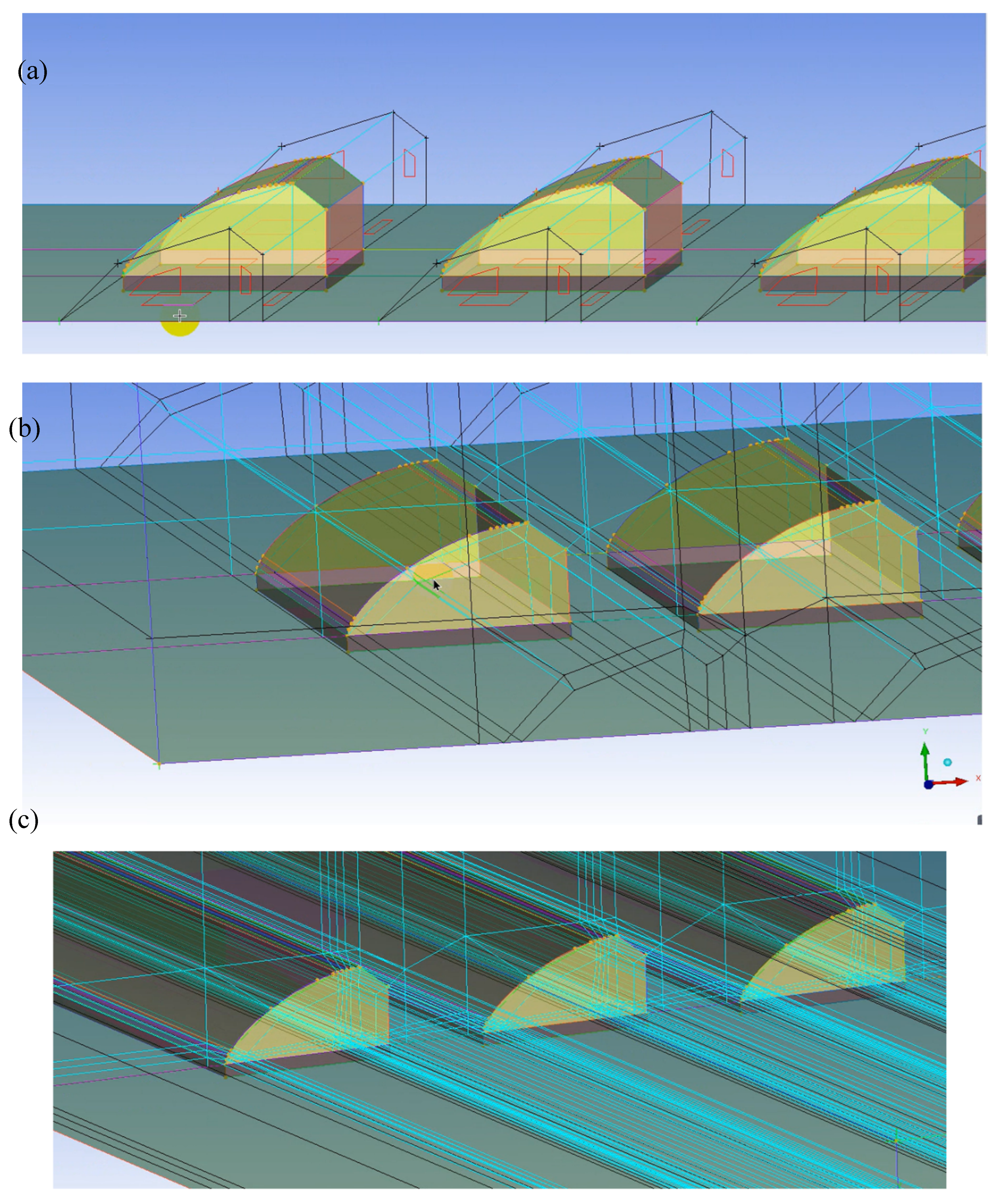
The first step in creating a mesh file is to build a geometric model. Then the geometric model is associated with created blocks, including associating Points with Vertex, associating Curves with Edges and associating Surfaces with Faces (
Figure 4 (a)). The former is the name corresponding to the geometric model, and the latter is the name corresponding to the block. The next key step is to split the blocks. Given the complexity of the semi fan-shaped south roof and in order to get a high-quality of the meshing of the boundary layer around, the ‘Ogrid Block’ splitting method was used along the side wall of the greenhouse (
Figure 4 (b)) [
35]. Finally, it is beneficial to move the vertex in order to find the optimal quality and check the global association (
Figure 4 (c)). The vertex movements were based on the geometric optimal solution under multiple criteria, e.g., avoiding sharp angles and reducing aspect ratios.
Tests of Grid Independence
The height of the first cell from the wall in the boundary layer was determined by conducting iteration tests of independence of the results regarding the grid density. The tested case corresponded to a windward flow for which a wind profile was imposed at the entrance of the calculation domain as follows [
38],
where, u is the wind speed, m s
-1; к is the von Karman constant, 0.42; H is the reference height, m; H
0 is the aerodynamic roughness length.
The turbulent kinetic energy k and dissipation rate ε distributions at the entrance are defined by the following equations [
39],
The wind speed at 2.5 m height (u2.5) was 5 m s-1 for the tested case. The criterion for the convergence residual was 1×10⁻³ for the continuity, k, and ε equations, and it was 1×10⁻⁶ for the energy equation.
The steady-state solution was generally reached within 500 steps for the 2D case and within 900 steps for the 3D case. The first cell height giving the optimum y+ solution was 0.025 m based on the iteration independence tests.
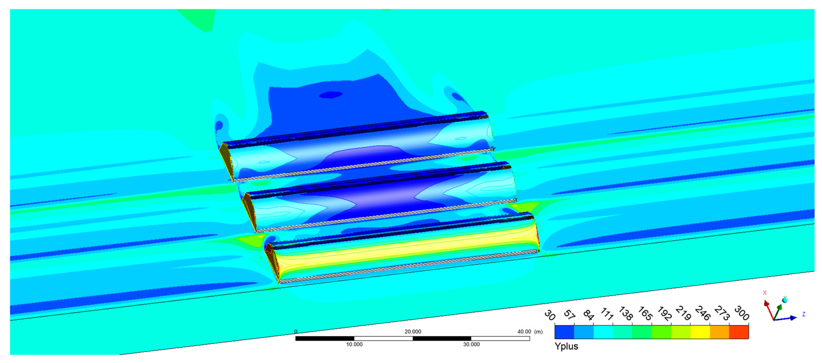
Figure 5 shows that the wall y+ satisfies 30<y
+<300 for the Standard Wall Function. The total number of elements is shown in
Table 3 and the mesh files are shown in
Figure 3 both for the windward and leeward cases.
2.5. Sample Data
In the first step, 2D and 3D modelling were conducted in parallel. 20 cases were selected (10 cases for 2D and 10 cases for 3D) to compare their natural ventilation rate and the wind field. The object is to experiment on the validity of 2D modellings when buildings are in rows. For these cases, the vents of the 3 greenhouses were fully open, with 30 m
2 opening areas for the upper and lower vents. Windward and leeward wind directions were applied, with a log law wind profile at the inlet (see
Table 4). Also, five values of the reference velocity u
2.5 from 1 to 5 m s
-1 were chosen for the simulations. The temperature difference between indoor and outdoor was 0 K (300 K inside both the indoor and outdoor domain). The ventilation rate through the vents of each greenhouse was monitored. The criterion of quality estimation of the fit between the 2D and the 3D models was defined as follows (Eq. 5),
where e is the ratio error; L
2 is the ventilation rate simulated by 2D case m
3 s
-1 and L
3 is the ventilation rate simulated by 3D case m
3 s
-1.
In the second step, 990 samples were collected using 2D simulations. The object is to study the greenhouse natural ventilation from a large sample size. These samples include natural ventilation rates under the coupling of gradient wind pressure, thermal pressure and vents opening combinations. A natural ventilation rate model was then developed using a nonlinear regression tree-model (see section 1.7). For these cases, there was only one greenhouse in the calculation domain. Eleven temperature differences between a fixed temperature of 300 K at the inlet and the average temperature inside the greenhouse from 0 to 10 K were tested. The steady indoor temperature was simulated by defining fixed wall temperature. The indoor average temperature was monitored by conducting iteration tests until it reached the targeted value. Combined with the 9 vent opening configurations described in
Table 1, windward and leeward directions were tested, with a log law wind profile at the inlet, and five values of u
2.5 from 1 to 5 m s
-1. This means in total 11*9*2*5=990 cases. The area ventilation rate was monitored and calculated by the following equations,
where L is the area ventilation rate, m
3 s
-1 m
-2; f
m is the simulated mass flow rate through the vents, kg m
-1 s
-1; l
g is the length of the greenhouse, m; A
g is the area of the greenhouse, m
2 and ρ is the density of the fluid (incompressible-ideal-gas), kg m
-3, which is calculated by the following equation [
35],
where R is the universal gas constant, 8.31 m
3 Pa K
-1 mol
-1; M
w is the molecular weight of the gas, kg mol
-1; P
op is the operating pressure, Pa.
2.6. Monitoring of Wind Speed at 2.5 M Height
Wind speed is a required parameter of the natural ventilation model. 2.5 m is usually a height that is easier for placing wind speed sensors on the outdoor weather stations. Meanwhile, wind speed at 2.5 m height (u
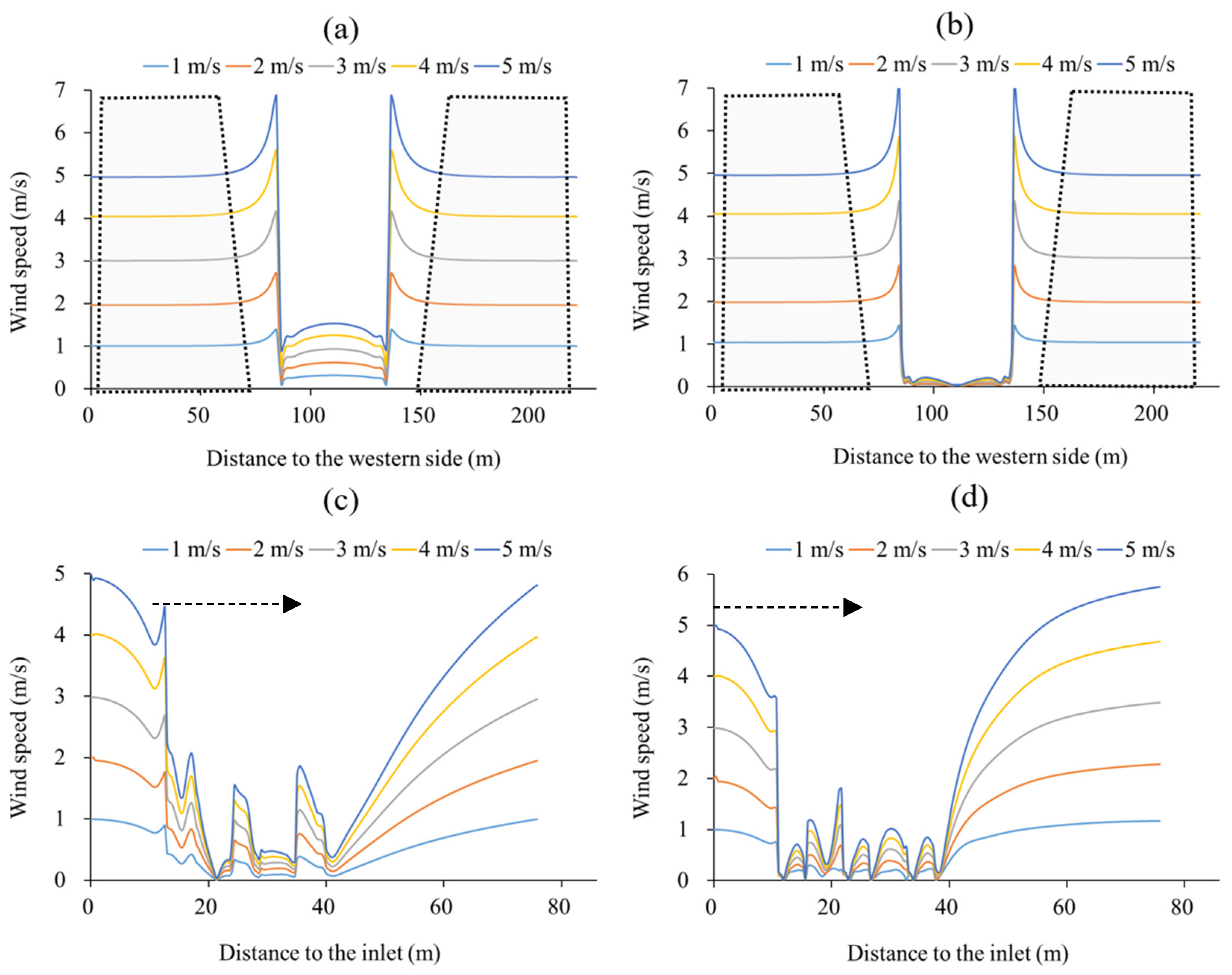
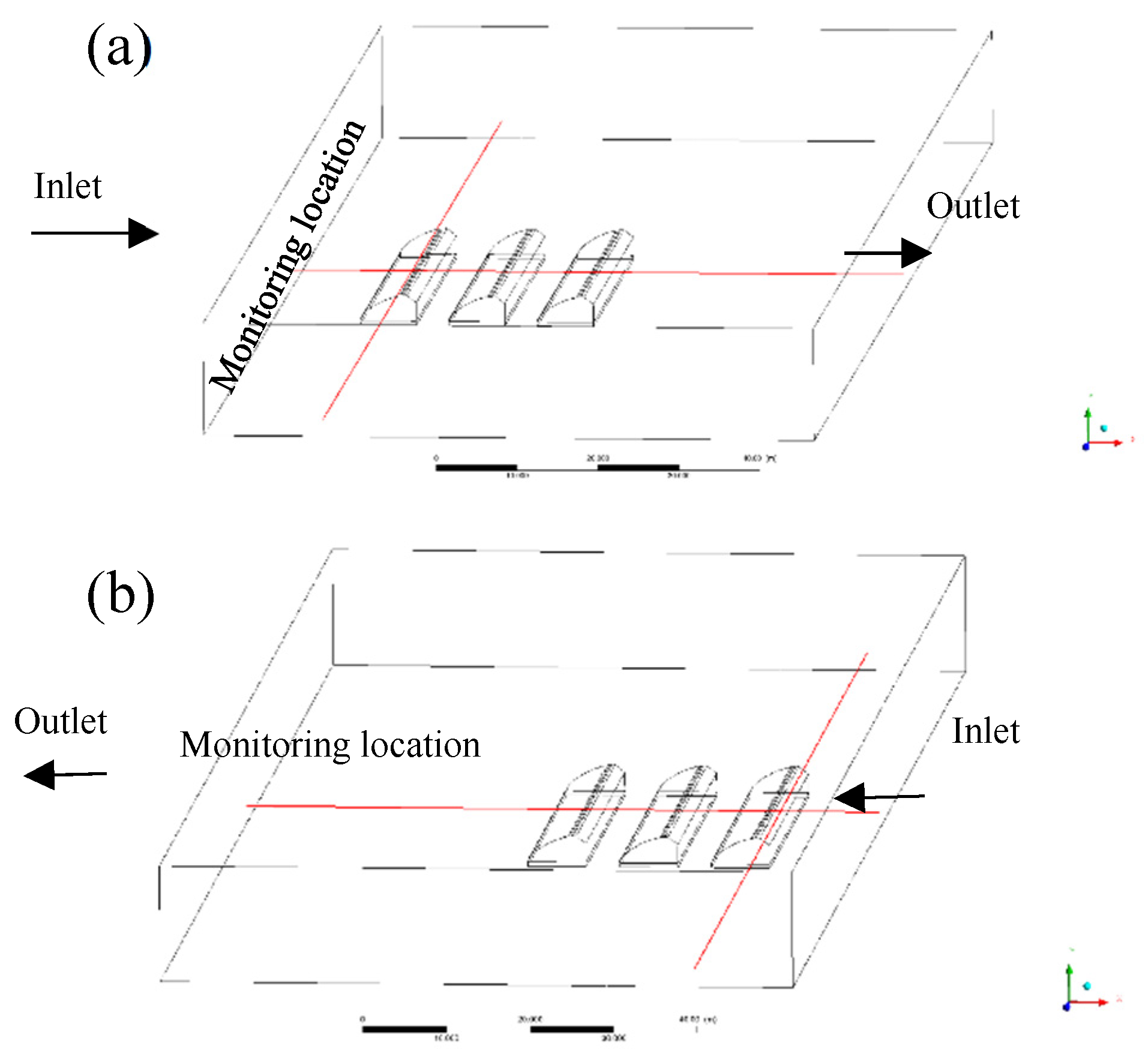
2.5) can be used to establish the inlet velocity profile. It is crucial to judge whether the measured wind speed is affected by buildings. Although, the appropriate distance of anemometers from objects is common knowledge in wind engineering. However, in most practice experiments, due to the variable structure of greenhouses and different experimental scenarios, it is necessary to specify a standard to provide a brief guidance for researchers who study the CSG climate prediction but have little knowledge in wind engineering. The method is to monitor the change of wind speed with position at the 2.5 m height horizontal plane, thus help to determine a limited area ensuring that the wind speed is in the free stream. The red lines in
Figure 6 show the monitoring locations at 2.5 m height, which cross the external domain and the whole greenhouse in two orthogonal directions. 10 groups of samples were monitored, which were respectively u
2.5 = 1~5 m s
-1 as the inlet inputs under windward and leeward flow.
2.7. Ventilation Model Establishment Using Regression Trees
Regression trees and classification trees belong to a particular kind of nonlinear predictive model, namely prediction trees. Regression trees are a way of making quantitative predictions, which use the trees to represent the recursive partition. Each of the leaves represents a cell of the partition and has attached to it a simple model which applies in that cell only [
40]. The inputs are respectively wind speed and directions, the upper and lower vent opening ratio areas (vent area/greenhouse area), and the temperature difference between indoor and outdoor. The output is the area ventilation rate, m
3 s
-1 m
-2. In this work, this technique has been used to obtain the natural ventilation rate model.
2.8. Statistics and Machin Learning Toolbox
MATLAB’s “Statistics and Machin Learning Toolbox” provides functions and applications to describe, analyze, and model data. It contains a Regression Trees Predict block that calculates responses to given input data. The regression trees model was trained and predicted by following the tree from the root node down to a leaf node. At each node, the model decides which branch to follow using the rule associated with that node and it continues until it arrives at a leaf node. Each step in a prediction involves checking the value of one predictor variable [
41].
2.9. Evaluation of the Regression Trees Ventilation Model
The evaluation of regression trees model was conducted to compare its output with an existing validated theoretical model used to simulate the ventilation rate of the CSG. The equations are shown below [
5], assume that the indoor and outdoor air temperatures distribution is uniform:
where
where, L
T is the thermal gradients ventilation rate, m
-3 s
-1; f
u is the coefficient of the thermal pressure ventilation rate; g is the gravitational acceleration, m s
-2; ∆H
v is the height difference between the upper vent and the lower vent, m; T is the indoor air temperature, K; T
o is the outdoor air temperature, K; u
j is the flow coefficient of the air inlet; F
j is the effective area of the air inlet, m
2; u
p is the flow coefficient of the air outlet; F
p is the effective area of the air outlet, m
2.
The wind pressure ventilation rate is estimated by an empirical value given by NY/T 1451-2018 [
42],
where, L
w is the wind pressure ventilation rate, m
-3 s
-1; β is the wind pressure coefficient.
The area ventilation rate was the square root of the quadratic sum divides area of the greenhouse,
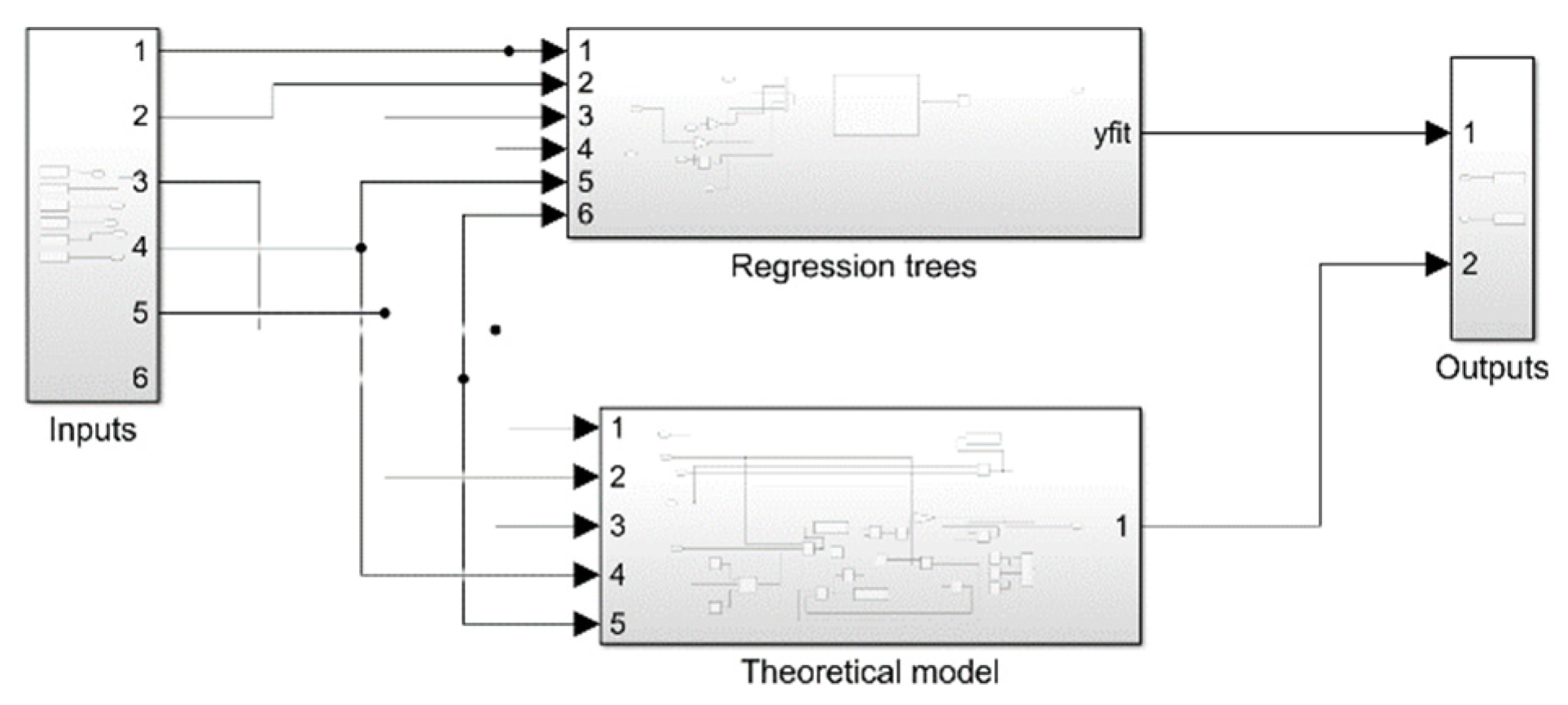
The evaluation was to calculate the averaged absolute error (AE) of predicted ventilation rate by entering the same inputs to the regression trees and the theoretical model, including gradient wind speeds, vent opening areas and temperature differences between indoor and outdoor, under leeward and windward conditions (
Figure 7).
3. Results and Discussion
This section describes the main results for the numerical analysis of the wind field in rows of the CSG, and the development of a natural ventilation model. First, the wind flow pattern around and inside multiple greenhouses and the ventilation rate are compared using 2D and 3D cases. Afterward, the limited area ensuring that the wind speed is in the free stream is demonstrated. Finally, a regression trees natural ventilation rate model is developed and evaluated.
3.1. Ventilation Rate and Airflow Pattern Under the Windward Condition
The airflow pattern is analyzed under windward conditions.
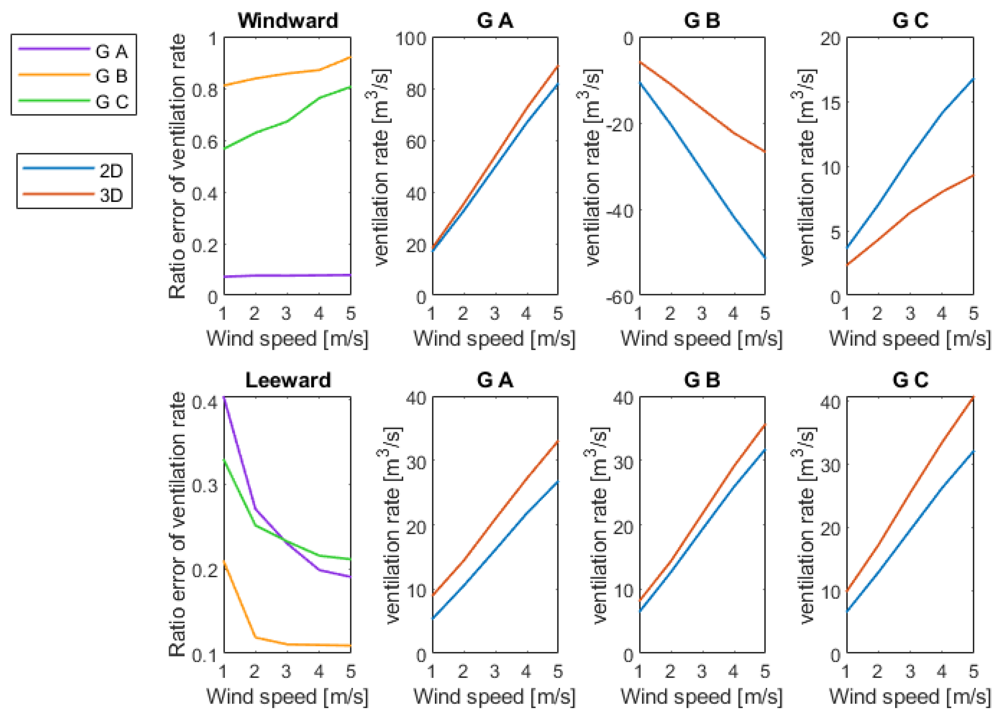
Figure 8 shows the comparative analysis between 2D and 3D cases. The vents openings are 100% in this comparative analysis section. The first row in
Figure 8 is for the windward condition. The ventilation rate of 2D and 3D are very close for the greenhouse A, for which the ratio errors are below 0.1 (
Figure 8) for 1-5 m s
-1 u
2.5 wind speeds. However, for greenhouses B and C (different positions in building clusters), the ratio errors are above 0.5. Besides, the errors for the greenhouse B are greater than the greenhouse C and it is positively correlated with wind speed. This result demonstrates that 2D cases are sufficient when there is no obstacle in front and behind the greenhouse in windward conditions. However, if there are other greenhouses in front and behind, 3D cases must be adopted.
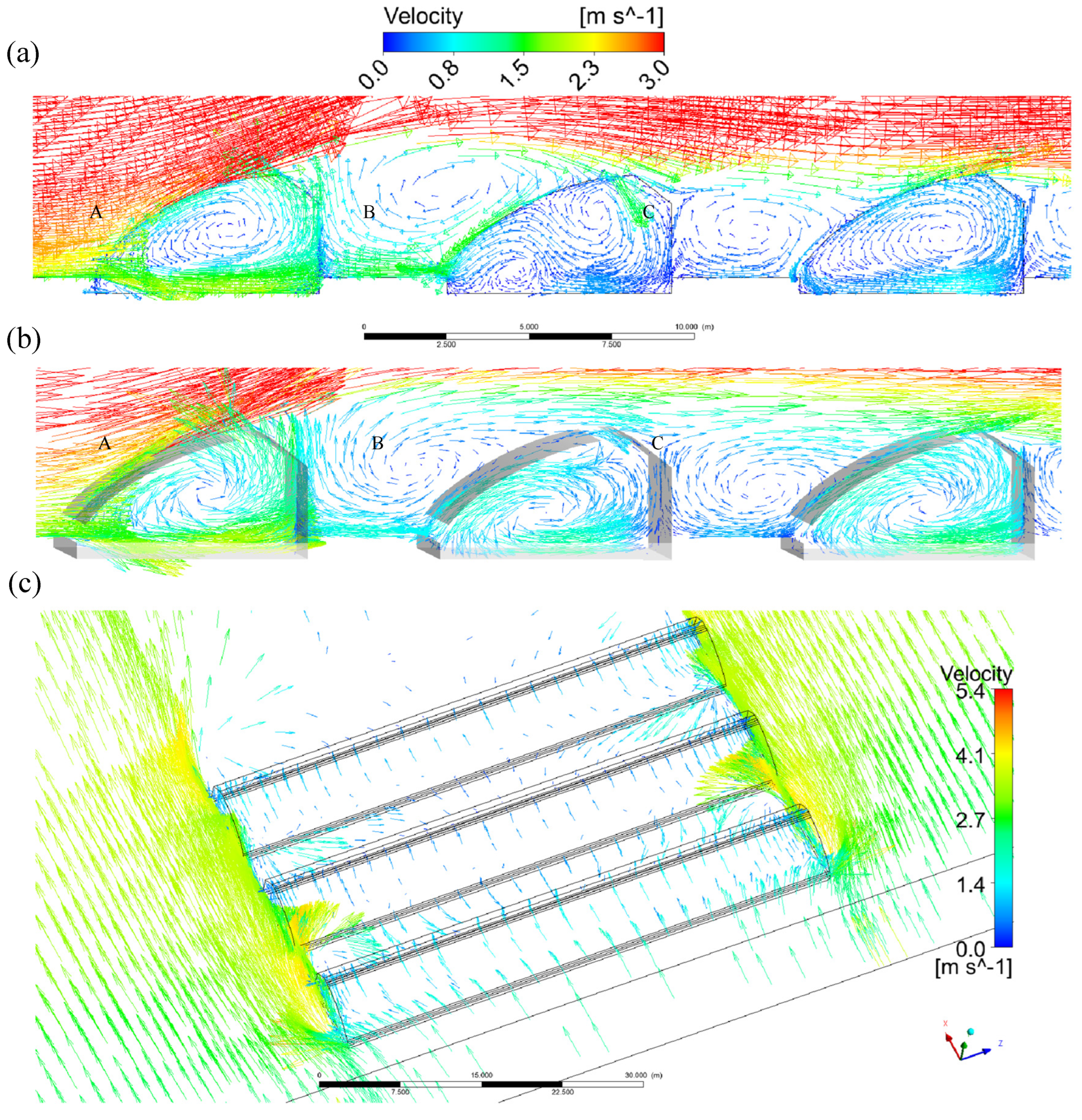
Figure 9 shows the velocity vectors obtained from 2D and 3D cases and depicts larger differences for the greenhouses B and C than for the A. The airflow patterns calculated from 2D and 3D simulations are indeed similar in the central vertical section of the front greenhouse of (
Figure 9 (a), (b)). From the results of the 3D case, it can be seen that the greenhouse in the back rows of the greenhouse cluster has a portion of the air intake coming from lateral sides of the greenhouse rows. This information is lost in 2D model. When adopting 2D case, for the middle and the back row greenhouses, the airflow pattern of the central section of the greenhouse thus cannot be regarded as that of the whole greenhouse. This fact explains why the middle and back row greenhouse has the great error in
Figure 9 regarding the ventilation rate prediction. This means also that if the 2D model is used for windward flow, there shall be no obstacles in front of and behind the greenhouse. Otherwise, the error could reach more than 50%.
From
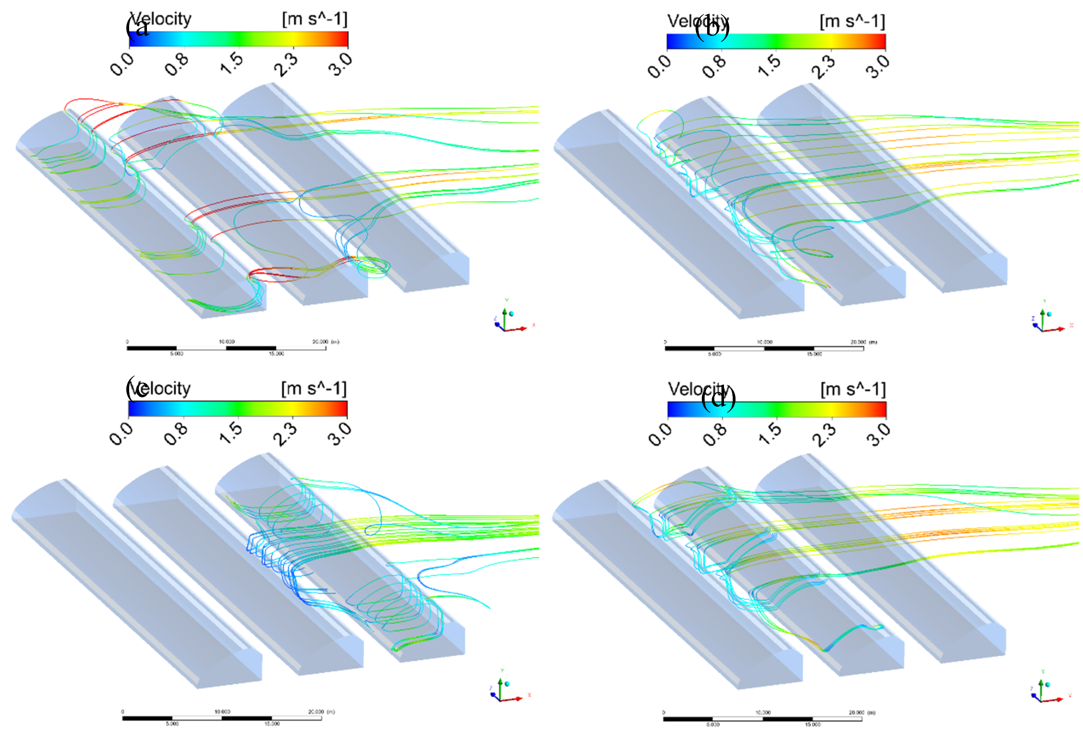
Figure 10 it can be seen that for greenhouse A, all air enters through the lower vent (
Figure 10 (a)). For greenhouse C, most of the air enters from the lower vent (
Figure 10 (c)). In the center of the greenhouse C, there is flow in the opposite direction. Nevertheless, the inflow of the lower vent is significantly greater than the outflow. For greenhouse B, most of the air enters the room from the upper vent and left from the lower vent (
Figure 10 (b), (d). Note that this result is related to the lack of thermal pressure, in addition, The flow pattern is affected by the turbulence model and time step size.
The above description is when the temperature difference inside and outside the greenhouse is 0 K, which means that wind pressure is dominant, the ventilation rate of greenhouse B is negative (
Figure 8). When thermal pressure is dominant, the flow pattern of greenhouse B changes.
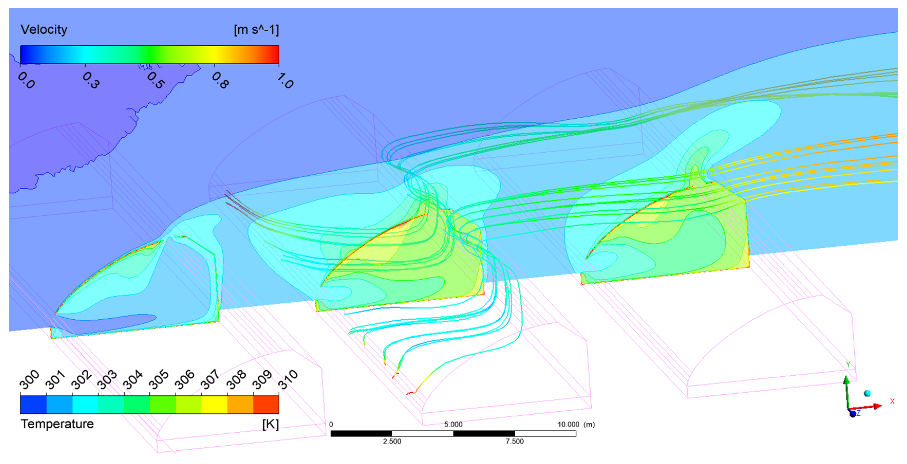
Figure 11 shows that when there is a temperature difference of about 5 K inside and outside the greenhouse, the upper vent is the outlet, and the ventilation rate is positive for greenhouse B. The wind speed is 1 m s
-1 and the ventilation rate is 6.5 m
3 s
-1. The thermal pressure also significantly increased the ventilation rate of greenhouse C from 2.3 m
3 s
-1 to 8.9 m
3 s
-1 under windward flow when u
2.5 is 1 m s
-1. This illustrates that in the greenhouse clusters, the influence of the wind pressure on the natural ventilation for the back rows greenhouses is limited. Appropriately increasing the spacing between greenhouses is therefore essential for maintaining ventilation.
3.2. Ventilation Rate and Airflow Pattern Under the Leeward Condition
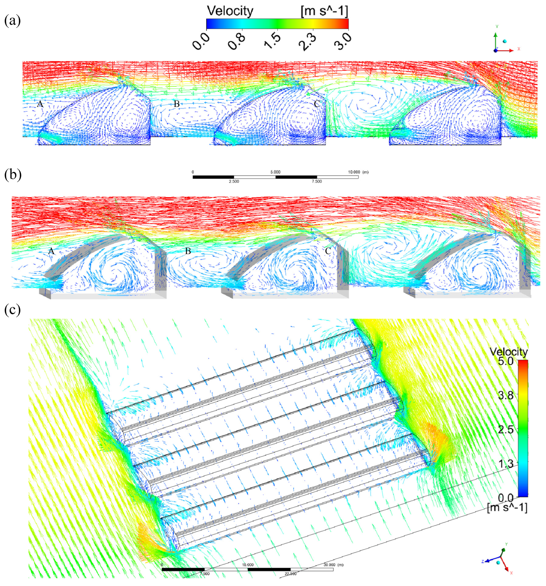
Under leeward flows, the lower vents are the inlet (
Figure 12 (a), (b)), and the ventilation rates from 3D simulations are greater than 2D in all the samples. This is probably because in 3D cases the inflow through lower vents comes from both the roof and lateral sides, whereas it comes only from the roof in 2D cases (
Figure 12 (c)). When adopting 2D simulation, this difference in the flow field is more enhanced inside the greenhouses A and C, than inside the greenhouse B. Besides, this impact is negatively correlated with wind speed. In general, the difference in natural ventilation rate simulation between 2D and 3D cases under leeward conditions is smaller than that under windward conditions. The ratio errors for greenhouse A, B, C in all the leeward flow cases were lower than 0.4. Among them, the greenhouse in the middle of the greenhouse rows has the smallest ratio errors, with a value between 0.1-0.2.
Current studies are aimed at a single greenhouse, ignoring the influence of surrounding buildings, and the wind direction is relatively simple [
23]. However, the modelling of flow fields in greenhouse clusters is of great relevance for both production and research in the future. Another reason for which most researchers choose 2D model is that their calculation is transient, and it is known that with three dimensional transient CFD simulation, it is difficult to achieve convergence at each time step, which affects the accuracy [
27,
43]. Although, with the progress of hardware, these problems are expected to be solved in the next few years, the methodology in this study looks forward to bringing time-consuming numerical computations into the fast transient simulation by training their results in the black box model.
3.3. Analysis of Wind Speed at the Monitoring Location
In the direction perpendicular to the wind, the impact of the building on the wind speed is positively correlated with wind speed (
Figure 13). The gray area in
Figure 13 (a), (b) shows the recommended area to place wind speed sensors ensuring that the measured wind is in free stream (the greenhouse wall is at 86 m from the western side) i.e. the area where the building does not impact the flow field anymore. Under the windward condition, the ranges where the wind speed changes sharply on both sides outside the greenhouse are below 8, 10, 16, 20, and 23 m away from the greenhouse under 1~5 m s
-1 wind speed respectively. Under the leeward condition, the distances are respectively below 7, 9, 13, 17, 20 m under 1~5 m s
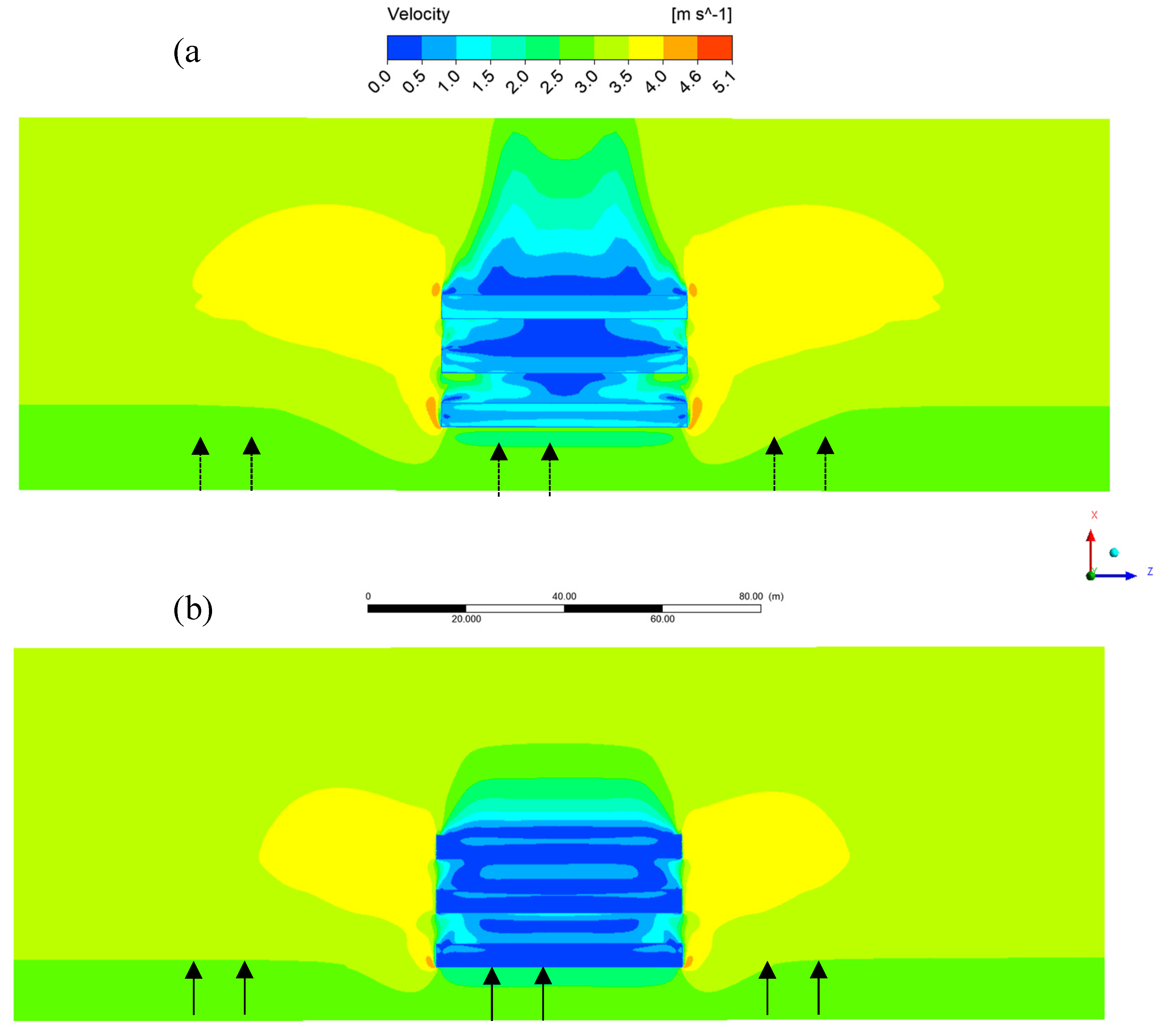
-1 wind speed. Beyond these distances, the measured wind speed is considered in the free stream. The impact of buildings on air flow on lateral sides is clearly seen from
Figure 14. This disturbance is more obvious for the greenhouse in the rear row. It is recommended to measure the free stream wind speed in the windward upstream of the building clusters.
In the direction parallel to the wind (the inlet is 10.8 m from the greenhouse), whether windward or leeward, the optimal distance to the greenhouse would be beyond 10.8 m (3 times the ridge height) in the upstream direction and above 36 m (10 times of the ridge height) in the downstream portion is 10 times, ensuring the wind speed is free (
Figure 13 (c), (d)). This conclusion was confirmed by Kim et al. [
34]. Measurements of the wind speed is a necessary step for simulating the greenhouse climate. Anemometers have to be placed in an open area outside of the greenhouse, this study gives the reference value of this distance in various cases.
3.4. Ventilation Model Establishment Using Regression Trees
Estimation of ventilation rate is a laborious work and usually requires multiple complex parameters. In this section, a regression trees ventilation model was developed from 990 CFD samples. This model applies to a greenhouse in an open area. Its inputs are the wind speed at a height of 2.5 m, the ratio area of the upper and lower vents, the area of the greenhouse, and the temperature difference between inside and outside of the greenhouse. The output is the area ventilation rate in m
3 s
-1 m
-2. The temperature difference was achieved by the imposed fixed wall temperature. The greenhouse temperature decreases from top to bottom, and an air temperature near the opaque walls higher than in other areas [
27]. By embedding the buoyancy equation, the contribution of thermal gradients to the ventilation rate is calculated by steady-state simulation.
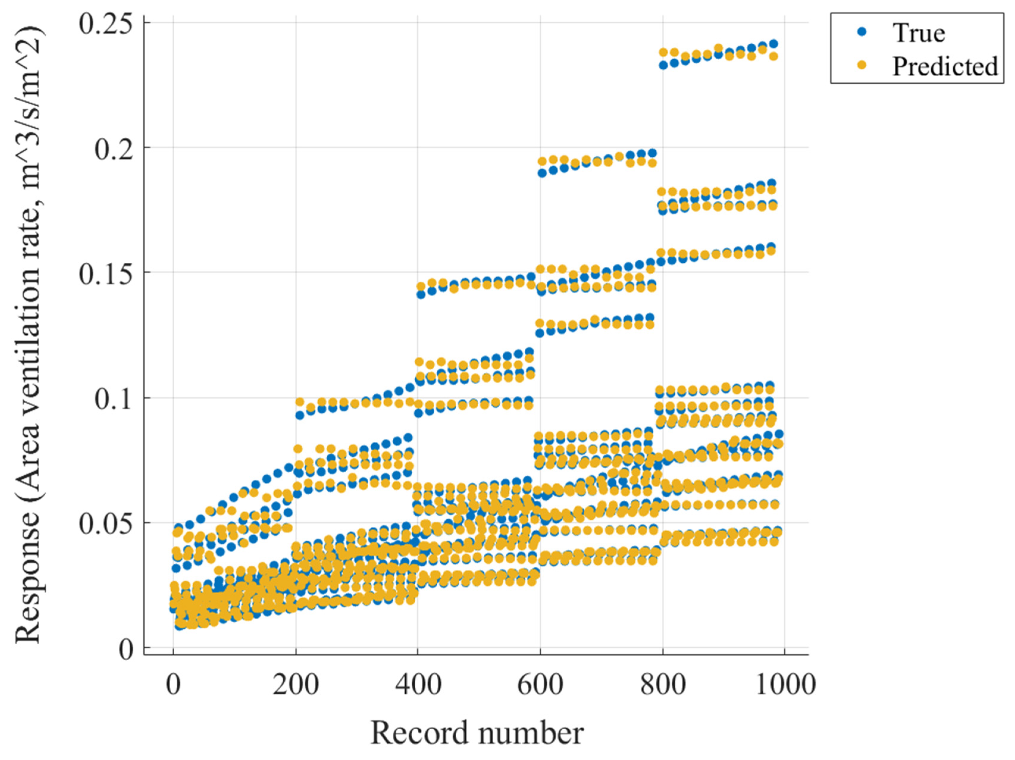
990 samples are used to train the model. In
Figure 15, the so-called “true” response is provided by CFD results while the predicted response is provided by the regression trees ventilation model. From left to right in
Figure 15, the velocity speed is increased, and from bottom to top, the vent opening area is increased. The points on each short line correspond to the tested temperature differences which increase from left to right. There are therefore consequently 11 points in each short line, representing the temperature difference between 0 to 10 K with a 1K temperature step. It shows that at low wind speed, the temperature difference makes the lines tilt greatly. But at high wind speeds, all the lines are almost horizontal, which demonstrates that under low wind speed, thermal pressure ventilation becomes predominant, and vice versa. From bottom to top, the vents opening areas are increased. There are 18 rows (9 vents combination * 2, windward and leeward) at each wind speed.
Figure 15 shows that choosing a larger vent area at high wind speed is more positive for increasing the ventilation rate than at low wind speed. The RMSE of the regression trees model is 0.002. This model can perfectly deal with the combined effect of wind pressure and thermal gradients.
3.5. Comparison Between the Regression Tree and Theoretical Models (eq. 11)
Figure 16 shows 330 pairs of samples. Each pair of samples is a comparison of the two models under the same input. The result shows that the curves of the regression trees and theoretical models are very close, with an AE between two models are 0.0077 m
3 s
-1 m
-2 (
Figure 16 (a)). From samples No.0-30, it is known that ventilation models are linear when the wind pressure is the only driving force. From samples No.31-330, the results show that the regression trees model can totally take over accurate predictions when the wind pressure and thermal pressure act simultaneously, without any theoretical parameters and laborious equation modeling.
4. Conclusions
This paper experimented with a methodology of machine learning modelling using virtual samples generated by a fast CFD (Computational Fluid Duy) simulations, in order to predict the greenhouse natural ventilation. Its main contributions may be summarized as follows:
- (i)
Three-dimensional simulations require a huge amount of computation load. It costs more than 30 hours to complete 900 iterations to achieve convergence in each 3D case, using an Intel Core I7 CPU and 16 GB RAM. For that reason, two-dimensional CFD simulations are still often adopted to study the wind flow pattern around the greenhouse. The present study compares 2D and 3D simulations, the results show that 2D model are sufficient when there is no obstacle in front and behind the greenhouse, especially in windward flows. But if there are other greenhouses nearby, 3D model should be adopted, Otherwise, the error could reach 50% on the ventilation rate prediction.
- (ii)
Turbulence around buildings makes it difficult to measure wind speed, this paper demonstrated limited area around rows of CSGs ensuring that the wind is in the free stream and gives the recommended distance to the greenhouse to place anemometers.
- (iii)
A regression trees natural ventilation model is developed using results from 990 two-dimensional CFD samples. This model perfectly deals with the combined effect of wind pressure and thermal gradients. This regression trees natural ventilation model is embedded in a published greenhouse model. The application shows this trees model performs ideal for a 7-day simulation (
Appendix A).
CFD method provides a theoretical basis for virtual wind tunnel experiments. A huge number of reliable samples can be obtained through virtual wind tunnel experiments. In the future, with the update of computer hardware, a refined ventilation model is looked forward to being trained through a large number of three-dimensional simulation results, including arbitrary wind direction and better accuracy.
Author Contributions
Conceptualization, R.L. (Ran Liu) and Y.S. (Yunyan Shi); data curation, R.L. and K.L. (Kaige Liu); methodology, R.L. and P.E.B. (Pierre-Emmanuel Bournet); software, R.L. and P.E.B. investigation, R.L. and Y.S.; writing—original draft preparation, R.L.; writing—review and editing, R.L., P.E.B. and Y.S.; visualization, R.L. and Y.S.; validation, R.L. and Y.S.; supervision, R.L.; project administration, R.L.; project acquisition, R.L. All authors have read and agreed to the published version of the manuscript.
Funding
This work has been funded by the Youth Project of the National Natural Science Foundation of China (32302453); Beijing Postdoctoral Research Foundation (2024-ZZ-092); Postdoctoral Research Project of the Beijing Academy of Agriculture and Forestry Sciences (2023-ZZ-010).
| Nomenclature |
|
qc
|
Convective energy, W |
| Ag
|
Area of the greenhouse, m2
|
qliq
|
Water vapor liquidation energy, W |
| cp
|
Specific heat capacity of the air, J kg-1 K-1
|
qp
|
Plant energy, W |
| cpw
|
Specific heat capacity of the water vapor, J kg-1 K-1
|
R |
Universal gas constant, m3 Pa K-1 mol-1
|
| e |
Ratio error |
sv
|
Ventilation humidity, kg kg-1 s-1
|
| Fj
|
Effective area of the air inlet, m2
|
slea
|
Air leakage humidity, kg kg-1 s-1
|
| Fp
|
Effective area of the air outlet, m2
|
sp
|
Plant humidity, kg kg-1 s-1
|
| fm
|
Simulated mass flow rate through the vents, kg m-1 s-1
|
T |
Indoor air temperature, K |
| fu
|
Coefficient of the thermal pressure ventilation rate |
To
|
Outdoor air temperature, K |
| g |
Gravitational acceleration, m s-2 |
t |
Time, s |
| H |
Reference height, m |
u |
Wind speed, m s-1
|
| H0
|
Aerodynamic roughness length, m |
uj
|
Flow coefficient of the air inlet |
| Hv |
Height between upper and lower vents, m |
up
|
Flow coefficient of the air outlet |
| h |
Indoor absolute humidity, kg kg-1
|
u2.5
|
Wind speed at 2.5 m height, m s-1
|
| L |
Area ventilation rate, m3 s-1 m-2
|
u*
|
Friction velocity, m s-1
|
| L2
|
Ventilation rate simulated by 2D case m3 s-1
|
v |
Greenhouse volume, m3
|
| L3
|
Ventilation rate simulated by 3D case m3 s-1
|
yc
|
Estimated height of the first cell in the boundary layer, m. |
| Lw
|
Wind pressure ventilation rate, m-3 s-1
|
y+
|
A non-dimensional distance |
| LT
|
Thermal gradients ventilation rate, m-3 s-1
|
β |
Wind pressure coefficient |
| lg
|
Length of the greenhouse, m |
μ |
Dynamic viscosity, Pa s-1
|
| Mw
|
Molecular weight of the gas, kg mol-1
|
ρ |
Air density, kg m-3
|
| Pop
|
Operating pressure, Pa |
к |
von Karman constant, 0.42 |
| qv(t) |
Ventilation energy, W |
|
|
| qlea(t) |
Air leakage energy, W |
|
|
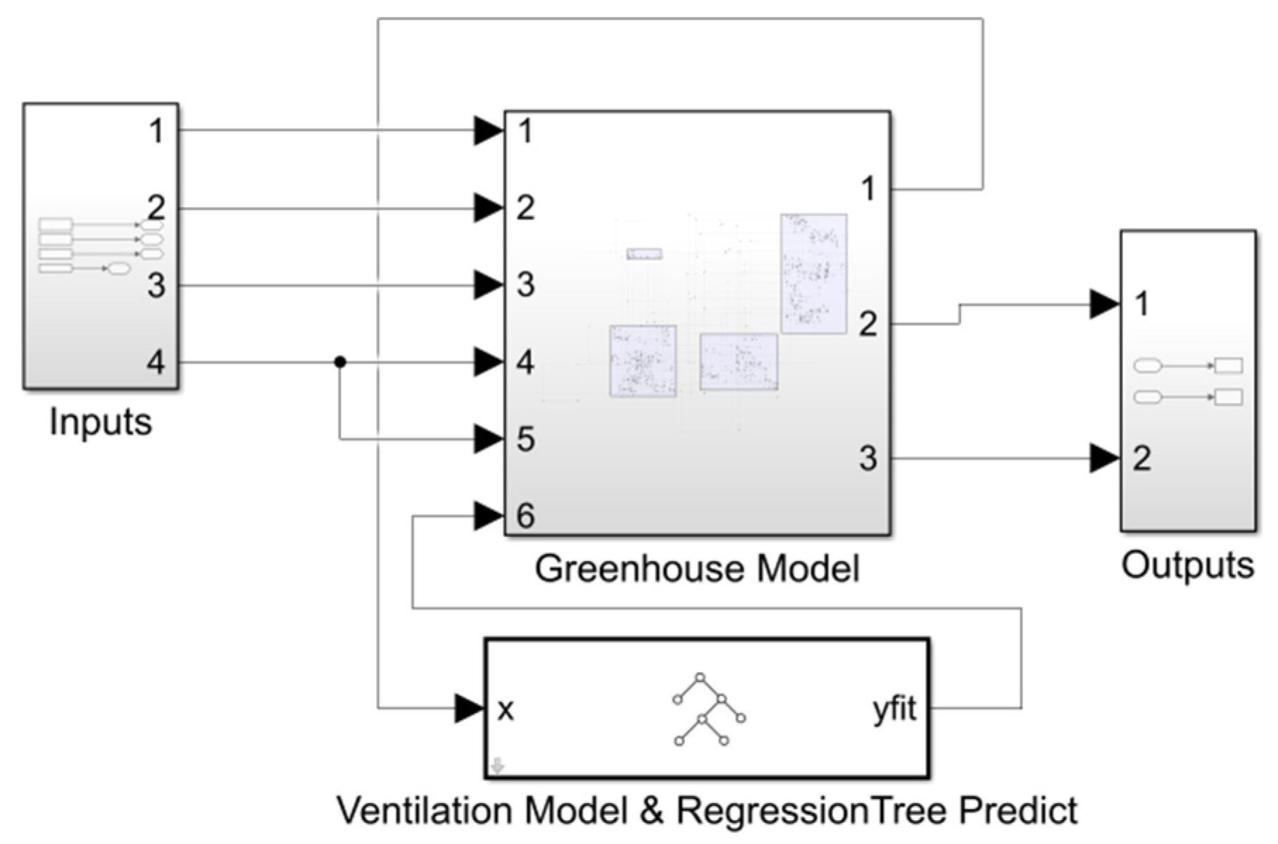
A brief introduction of the application about the regression tree ventilation model is shown in
Figure A1. The developed regression trees model was connected to a one-dimensional greenhouse model that can predict the temperature and humidity (Fig. A1) [
6]. The energy source terms for the air in the greenhouse are associated with 5 sub-mechanisms: the ventilation energy, q
v(t), W; the air leakage energy, q
lea(t), W; the convective energy, q
c(t), W; the water vapor-liquid transfer energy, q
liq(t), W; and the plant energy, q
p(t), W. The corresponding equation is given below:
where, h is the indoor absolute humidity, kg kg
-1; t is time, s; ρ is the air density, (1.293) kg m
-3; c
p is the specific heat capacity of the air, (1005) J kg
-1 K
-1; c
pw is the specific heat capacity of the water vapor, (1850) J kg
-1 K
-1; and
is the greenhouse volume, m
3. The greenhouse humidity source terms come from the ventilation humidity, s
v(t), kg kg
-1 s
-1; the air leakage humidity, s
lea(t), kg kg
-1 s
-1; and the plant humidity, s
p(t), kg kg
-1 s
-1. The equation is given as follows,
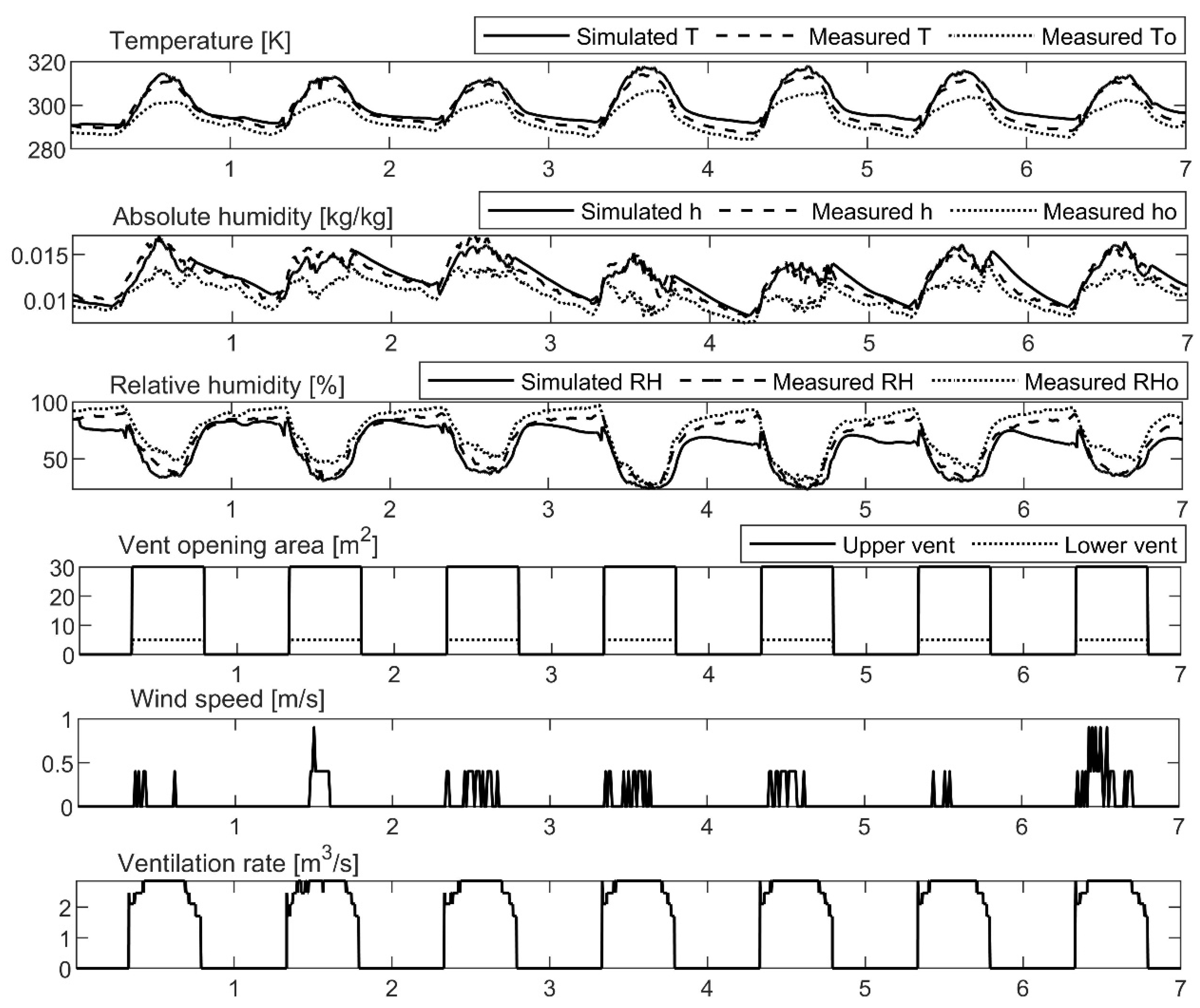
The application was presented and validated using a new group of measured climate data collected on 20-26 Sept. 2019 from inside and outside of the greenhouse. The greenhouse is the same size as
Figure 2, and it is located in Xiaotangshan, at the National Precision Agriculture Demonstration Base (40°18’ N, 116°47’ E), Changping District, Beijing, China. The outdoor climate data, including temperature, relative humidity, solar radiation, wind speed, and direction, was measured every 15 mins to provide input to the greenhouse model. The vents were opened from 7:00-18:00 during the experimental days. The upper and lower opening area were respectively 30 m
2 and 5 m
2. The indoor temperature and humidity were measured every 15 mins to be validated with the predictions using root mean squared error (RMSE).
Figure A1.
Application of regression trees model.
Figure A1.
Application of regression trees model.
Figure A2 shows results obtained from a fast one-dimensional transient greenhouse model, in which the regression trees ventilation model was included. Comparisons between measurements and simulations are provided for September 20-26, 2019. The results show that the model performs well as RMSE of temperature and relative humidity of 3.2 K and 9.8% respectively were found for a 7-day simulation.
Figure A2.
Data set used for the model validation with the temperature and humidity on September 20-26, 2019. T is the averaged indoor temperature, K; To is the outdoor temperature, K; h is the averaged indoor absolute humidity, kg kg-1; ho is the outdoor absolute humidity, kg kg-1; RH is the averaged indoor relative humidity, %; RHo is the outdoor relative humidity, %.
References
- Wu, G., Yang, Q., Zhang, Y., Fang, H., Feng, C., Zheng, H., 2020. Energy and optical analysis of photovoltaic thermal integrated with rotary linear curved Fresnel lens inside a Chinese solar greenhouse. Energy. 197, 117215. [CrossRef]
- Lei, W., Lu, H., Qi, X., Tai, C., Fan, X., Zhang, L., 2023. Field measurement of environmental parameters in solar greenhouses and analysis of the application of passive ventilation. Sol Energ. 263, 111851. [CrossRef]
- Cheng, X., Li, D., Shao, L., Ren, Z., 2021. A virtual sensor simulation system of a flower greenhouse coupled with a new temperature microclimate model using three-dimensional CFD. Computers and Electronics in Agriculture. 181, 105934. [CrossRef]
- Li, T., Chang, J., Wei, M., Shi, G., Zhang, Y., Chen, D., 2018. Application situation and problem analysis of ventilation facilities in solar greenhouse in Shandong province. Agricultural Engineering and Technology. 38(16), 22-26. (In Chinese) . [CrossRef]
- Zhang, G., Fu, Z., Yang, M., Liu, X., Dong, Y., Li, X., 2019. Nonlinear simulation for coupling modeling of air humidity and vent opening in Chinese solar greenhouse based on CFD. Computers and Electronics in Agriculture. 162, 337-347. [CrossRef]
- Liu, R., Li, M., Guzmán, J.L., Rodríguez, F., 2021. A fast and practical one-dimensional transient model for greenhouse temperature and humidity. Computers and Electronics in Agriculture. 186, 106186. [CrossRef]
- Mistriotis. A., Bot, G.P.A., Picuno, P., Scarascia-Mugnozza, G., 1997. Analysis of the efficiency of greenhouse ventilation using computational fluid dynamics. Agricultural and Forest Meteorology. 85(3–4), 217-228. [CrossRef]
- Ould Khaoua, S.A., Bournet, P.E., Migeon, C., Boulard, T., Chassériaux, G., 2006. Analysis of Greenhouse Ventilation Efficiency based on Computational Fluid Dynamics. Biosystems Engineering. 95(1), 83-98. [CrossRef]
- Katsoulas, N., Bartzanas, T., Boulard, T., Mermier, M., Kittas, C., 2006. Effect of vent openings and insect screens on greenhouse ventilation. Biosystems Engineering. 93(4), 427-436. [CrossRef]
- Nederhoff, E.M., van de Vooren, J., Udink ten Cate, A.J., 1985. A practical tracer gas method to determine ventilation in greenhouses. Journal of Agricultural Engineering Research. 31(4), 309-319. [CrossRef]
- Tong, G., Che, Z., Bai, Y., Yamaguchi, T., 2008. Air exchange rate calculation for solar greenhouse using thermal balance method. Journal of Shenyang Agricultural University. 39(4), 459-462. (In Chinese) . [CrossRef]
- Van Buggenhout, S., Ozcan, S.E., Vranken, E., Van Malcot, W., Berckmans, D., 2007. Acoustical Ventilation Rate Sensor Concept for Naturally Ventilated Buildings. ASHRAE Transactions. 113(2), 192–199.
- Boulard, T., Roy, J.C., Lamrani, M.A., Haxaire, R., 1997. Characterising and Modelling the Air Flow and Temperature Profiles in a Closed Greenhouse in Diurnal Conditions. IFAC Proceedings Volumes. 30(26), 37-42. [CrossRef]
- Boulard, T., Wang, S., 2002. Experimental and numerical studies on the heterogeneity of crop transpiration in a plastic tunnel. Computers and Electronics in Agriculture. 34(1-3), 173-190. [CrossRef]
- Majdoubi, H., Boulard, T., Fatnassi, H., Bouirden, L., 2009. Airflow and microclimate patterns in a one-hectare Canary type greenhouse: An experimental and CFD assisted study. Agricultural and Forest Meteorology. 149(6–7), 1050-1062. [CrossRef]
- Boulard, T., Roy, J.C., Fatnassi, H., Kichah, A., Lee, I.-B., 2010. Computer fluid dynamics prediction of climate and fungal spore transfer in a rose greenhouse. Computers and Electronics in Agriculture. 74(2), 280-292. [CrossRef]
- Kichah, A., Bournet, P.-E., Migeon, C., Boulard, T., 2012. Measurement and CFD simulation of microclimate characteristics and transpiration of an Impatiens pot plant crop in a greenhouse. Biosystems Engineering. 112(1), 22–34. [CrossRef]
- Chen, J., Xu, F., Tan, D., Shen, Z., Zhang, L., Ai, Q., 2015. A control method for agricultural greenhouses heating based on computational fluid dynamics and energy prediction model. Applied Energy. 141, 106-118. [CrossRef]
- Boulard, T., Roy, J.C., Pouillard, J.B., Fatnassi, H., Grisey, A., 2017. Modelling of micrometeorology, canopy transpiration and photosynthesis in a closed greenhouse using computational fluid dynamics. Biosystems Engineering. 158, 110-133. [CrossRef]
- Liu, R., Liu, J., Liu, H., Yang, X., Bienvenido Bárcena, J.F., Li, M., 2021. A 3-D simulation of leaf condensation on cucumber canopy in a solar greenhouse. Biosystems Engineering. 210, 310-329. [CrossRef]
- Molina-Aiz, F.D., Fatnassi, H., Boulard, T., Roy, J.C., Valera, D.L., 2010. Comparison of finite element and finite volume methods for simulation of natural ventilation in greenhouses. Computers and Electronics in Agriculture. 72(2), 69-86. [CrossRef]
- Rocha, G.A.O., Pichimata, M.A., Villagran, E., 2021. Research on the Microclimate of Protected Agriculture Structures Using Numerical Simulation Tools: A Technical and Bibliometric Analysis as a Contribution to the Sustainability of Under-Cover Cropping in Tropical and Subtropical Countries. Sustainability. 13, 10433. [CrossRef]
- Bournet, P.-E., Boulard, T., 2010. Effect of ventilator configuration on the distributed climate of greenhouses: A review of experimental and CFD studies. Computers and Electronics in Agriculture. 74(2), 195-217. [CrossRef]
- Villagrán, E.A., Baeza Romero, E.J., Bojacá, C.R., 2019. Transient CFD analysis of the natural ventilation of three types of greenhouses used for agricultural production in a tropical mountain climate. Biosystems Engineering. 188, 288-304. [CrossRef]
- Benni, S., Tassinari, P., Bonora, F., Barbaresi, A., Torreggiani, D., 2016. Efficacy of greenhouse natural ventilation: Environmental monitoring and CFD simulations of a study case. Energy and Buildings. 125, 276-286. [CrossRef]
- Wang, X., Luo, J., Li, X., 2013. CFD Based Study of Heterogeneous Microclimate in a Typical Chinese Greenhouse in Central China. Journal of Integrative Agriculture. 12(5), 914-923. [CrossRef]
- He, X., Wang, J., Guo, S., Zhang, J., Wei, B., Sun, J., Shu, S., 2018. Ventilation optimization of solar greenhouse with removable back walls based on CFD. Computers and Electronics in Agriculture. 149, 16-25. [CrossRef]
- Bournet P.E., Rojano F., 2022. Advances of Computational Fluid Dynamics (CFD) applications in agricultural building modelling: research, applications and challenges, Computers and Electronics in Agriculture, 201(5):107277. [CrossRef]
- Zhang, X., Wang, H., Zou, Z., Wang, S., 2016. CFD and weighted entropy based simulation and optimisation of Chinese Solar Greenhouse temperature distribution. Biosystems Engineering. 142, 12-26. [CrossRef]
- Villagrán, E.A., Bojacá, C.R., 2019. Effects of surrounding objects on the thermal performance of passively ventilated greenhouses. Journal of Agricultural Engineering. 856, 20-27. http://hdl.handle.net/20.500.12010/8700.
- Kim, R.-w., Hong, S.-w., Norton, T., Amon, T., Youssef, A., Berckmans, D., Lee, I.-b., 2020. Computational fluid dynamics for non-experts: Development of a user-friendly CFD simulator (HNVR-SYS) for natural ventilation design applications. Biosystems Engineering. 193, 232-246. [CrossRef]
- Kim, R.-w., Kim, J.-g., Lee, I.-b., Yeo, U.-h., Lee, S.-y., Decano-Valentin, C., 2021. Development of three-dimensional visualisation technology of the aerodynamic environment in a greenhouse using CFD and VR technology, part 1: Development of VR a database using CFD, Biosystems Engineering. 207, 33-58. [CrossRef]
- Fehér, T., 2006. Using Regression Trees in Predictive Modelling. Production Systems and Information Engineering. 4, 115-124.
- Kim, R.-w., Lee, I.-b., Kwon, K.-s., 2017. Evaluation of wind pressure acting on multi-span greenhouses using CFD technique, Part 1: Development of the CFD model. Biosystems Engineering. 164, 235-256. [CrossRef]
- Ansys. 2010. Ansys Fluent User’s guide. Ansys, Inc., Canonsburg, PA, USA ed.
- Piscia, D., Montero, J.I., Baeza, E., Bailey, B.J., 2012. A CFD greenhouse night-time condensation model. Biosystems Engineering. 111(2), 141-154. [CrossRef]
- Toparlar, Y., Blocken, B., Maiheu, B., van Heijst, G., 2019. CFD simulation of the near-neutral atmospheric boundary layer: New temperature inlet profile consistent with wall functions. Journal of Wind Engineering and Industrial Aerodynamics. 191, 91-102. [CrossRef]
- Haxaire, R., 1999. Caractérisation et modélisation des écoulements d’air dans une serre. Ph.D. Thesis. Université de Nice, France.
- Hoxey, R.P., Richardson, G.M., 1983. Measurements of wind loads on full scale plastic greenhouse. J. Wind Eng. Ind. Aerodynam. 16, 57–83.
- Shalizi, C., 2006. Statistics 36-350: Data Mining. Lecture 10: Regression Trees. https://www.stat.cmu.edu/~cshalizi/350-2006/.
- MATLAB user’s manual, R2021b. 2021.
- NY/T 1451-2018, 2018. Code for ventilation design of greenhouse. Ministry of Agriculture of the PRC. P:7-8. (In Chinese).
- Tong, G., Christopher, D.M., Zhang, G., 2018. New insights on span selection for Chinese solar greenhouses using CFD analyses. Computers and Electronics in Agriculture. 149, 3-15. [CrossRef]
Figure 1.
Chinese solar greenhouse rows, Beijng.
Figure 1.
Chinese solar greenhouse rows, Beijng.
Figure 2.
Structure of the experimental greenhouse.
Figure 2.
Structure of the experimental greenhouse.
Figure 3.
Mesh of windward and leeward flow field and greenhouses A, B, C. The difference between windward and leeward mesh is lies in the length computational domains in front and behind the greenhouse.
Figure 3.
Mesh of windward and leeward flow field and greenhouses A, B, C. The difference between windward and leeward mesh is lies in the length computational domains in front and behind the greenhouse.
Figure 4.
Process of creating a mesh file. (a) is the process of creating Ogrid Block; (b) is the result of the roof boundary layer block; (c) is the final global block split result.
Figure 4.
Process of creating a mesh file. (a) is the process of creating Ogrid Block; (b) is the result of the roof boundary layer block; (c) is the final global block split result.
Figure 5.
Wall y+ value for the case where the first cell height is 0.025 m.
Figure 5.
Wall y+ value for the case where the first cell height is 0.025 m.
Figure 6.
Monitoring location (red lines) of wind speed, (a) for windward flow, and (b) for leeward flow.
Figure 6.
Monitoring location (red lines) of wind speed, (a) for windward flow, and (b) for leeward flow.
Figure 7.
Comparison of predicted ventilation rate between the regression trees and theoretical models.
Figure 7.
Comparison of predicted ventilation rate between the regression trees and theoretical models.
Figure 8.
Ratio error of ventilation rate between 2D and 3D cases under windward and leeward conditions. Ventilation rate from 2D and 3D cases for each greenhouse. G A, G B, G C are respectively greenhouse A, B and C. See
Figure 3 for positions of greenhouses A, B, C. Negative value means that the lower vent is a net outflow.
Figure 9.
Velocity vectors of windward flow when u2.5 is 3 m s-1. (a) from 2D simulation and (b) at the same location from 3D simulation. (c) top view at lower vents height from 3D simulation.
Figure 9.
Velocity vectors of windward flow when u2.5 is 3 m s-1. (a) from 2D simulation and (b) at the same location from 3D simulation. (c) top view at lower vents height from 3D simulation.
Figure 10.
Streamlines of windward flow when u2.5 is 3 m s-1. (a), (b) and (c) are for greenhouse A, B and C, where streamlines start from the lower vents. (d) is for the greenhouse B, where streamlines start from the upper vents.
Figure 10.
Streamlines of windward flow when u2.5 is 3 m s-1. (a), (b) and (c) are for greenhouse A, B and C, where streamlines start from the lower vents. (d) is for the greenhouse B, where streamlines start from the upper vents.
Figure 11.
Streamlines of windward flow when u2.5 is 1 m s-1, and temperature contour for greenhouse B.
Figure 11.
Streamlines of windward flow when u2.5 is 1 m s-1, and temperature contour for greenhouse B.
Figure 12.
Velocity vectors of leeward flow when u2.5 is 3 m s-1. (a) is from 2D simulation and (b) is the same location from 3D simulation. (c) is the overhead view at lower vents height from 3D simulation.
Figure 12.
Velocity vectors of leeward flow when u2.5 is 3 m s-1. (a) is from 2D simulation and (b) is the same location from 3D simulation. (c) is the overhead view at lower vents height from 3D simulation.
Figure 13.
Wind speed at the monitoring location. (a) (c) are under windward flow, (b) (d) are under leeward flow. (a) (b) are located perpendicular to the wind direction at 2.5 m height in the middle E-W cross section of the greenhouse. (c) (d) are located parallel to the wind direction at 2.5 m height in the middle N-S cross section. The gray area is the recommended area to place wind speed sensors.

is the wind direction.
Figure 13.
Wind speed at the monitoring location. (a) (c) are under windward flow, (b) (d) are under leeward flow. (a) (b) are located perpendicular to the wind direction at 2.5 m height in the middle E-W cross section of the greenhouse. (c) (d) are located parallel to the wind direction at 2.5 m height in the middle N-S cross section. The gray area is the recommended area to place wind speed sensors.

is the wind direction.
Figure 14.
Contour of wind speed on the 2.5 m height horizontal plane. (a) is windward flow and (b) is leeward flow.
Figure 14.
Contour of wind speed on the 2.5 m height horizontal plane. (a) is windward flow and (b) is leeward flow.
Figure 15.
Responses of regression trees ventilation model: predicted vs actual plot.
Figure 15.
Responses of regression trees ventilation model: predicted vs actual plot.
Figure 16.
Comparison of predicted ventilation rate between the regression trees and theoretical models. (a) is outputs and (b) is inputs. Wind speeds range 1-5 m s-1 (purple line); temperature differences range 0-10 K (red line); equally vent opening area for the upper and lower vents, respectively 10, 20, 30 m2 (green line); 0 represents windward and 1 represents leeward (orange line). The β value of the theoretical model is 0.5 under windward flow and 0.2 under leeward flow for Eq. 10.
Table 1.
Simulated greenhouse size and vent opening configurations.
Table 1.
Simulated greenhouse size and vent opening configurations.
Width
(m) |
Ridge Height
(m) |
Length
(m) |
Depth
(m) |
Vent Type |
Vent Opening Area (m2) |
| Lower Vent |
Upper Vent |
| 7 |
3.6 |
50 |
0.5 |
Rolling Film |
10 |
10 |
| 20 |
| 30 |
| 20 |
10 |
| 20 |
| 30 |
| 30 |
10 |
| 20 |
| 30 |
Table 2.
Physical properties of the air.
Table 2.
Physical properties of the air.
| Material |
Density
(kg m-3) |
Specific Heat
(J kg-1 K-1) |
Thermal Conductivity
(W m-1 K-1) |
Viscosity
(kg m-1 s-1) |
| Air |
Incompressible-ideal-gas |
1006 |
0.024 |
1.7894×10⁻⁵
|
Table 3.
Number of elements of the 2D and 3D Meshes.
Table 3.
Number of elements of the 2D and 3D Meshes.
| Mesh |
Windward Mesh |
Leeward Mesh |
| 2D |
36722 |
36726 |
| 3D |
16807531 |
16776673 |
Table 4.
Boundary conditions.
Table 4.
Boundary conditions.
| Boundary |
Boundary Condition |
| Momentum |
Thermal |
| Wall |
No-slip wall |
Fixed temperature |
| South roof |
No-slip wall |
Fixed temperature |
| North roof |
No-slip wall |
Fixed temperature |
| Ground |
No-slip wall |
Fixed temperature |
| External top, both sides |
Symmetry |
| Inlet of the external domain |
Velocity-inlet: Wind profile Eq. 2, 3, 4; Temperature 300 K |
| Outlet of the external domain |
Pressure-outlet; Temperature 300 K |
|
Disclaimer/Publisher’s Note: The statements, opinions and data contained in all publications are solely those of the individual author(s) and contributor(s) and not of MDPI and/or the editor(s). MDPI and/or the editor(s) disclaim responsibility for any injury to people or property resulting from any ideas, methods, instructions or products referred to in the content. |
© 2024 by the authors. Licensee MDPI, Basel, Switzerland. This article is an open access article distributed under the terms and conditions of the Creative Commons Attribution (CC BY) license (http://creativecommons.org/licenses/by/4.0/).

 is the wind direction.
 is the wind direction.