Preprint
Article

Multi-Modal Deep Learning Architecture for Improved Colposcopy Image Classification

This version is not peer-reviewed.

Submitted:

01 November 2024

Posted:

04 November 2024

You are already at the latest version

Abstract
Colposcopy image classification is vital for early cervical cancer detection, yet it remains challenging due to the significant variation in lesion appearances. Although deep learning models have advanced medical image classification, few studies have explored combining different model architectures to enhance diagnostic accuracy in colposcopy. This study addresses this gap by proposing a lesion-specific, multi-branch architecture that integrates attention mechanisms, deep feature extraction, and ensemble learning. Multi-task learning is employed to manage multiple lesion-specific classification tasks, while an ensemble of classifiers—Logistic Regression, XGBoost, and CatBoost—enhances decision-making accuracy. The architecture includes deep learning branches using EfficientNetB0 and MobileNetV2 for rich feature extraction from colposcopy images, with their outputs combined through a soft voting ensemble. Hyperparameter tuning, k-fold cross-validation, PCA visualization, and AUC plots for multiclass performance were used to optimize and assess model effectiveness. Training and validation accuracy were tracked in two phases: after the training phase, training accuracy reached 97.85\% and validation accuracy was 97.33\%; after the final ensemble classification, training accuracy improved to 99.95\% and validation accuracy to 99.85\%, surpassing individual model performance and demonstrating enhanced generalization. This model shows substantial promise for improving colposcopy classification accuracy, providing a valuable tool for clinical decision support in cervical cancer diagnosis.
Keywords: 
Subject: 
Engineering  -   Other

1. Introduction

Despite being preventable if caught early, women are disproportionately affected by cervical cancer globally [1]. It happens when abnormal cells around the womb develop into cancer, mainly because of HPV. Within the cervix, glandular cells give way to squamous cells through a normal process [2]. These cells may develop abnormalities and eventually turn into cancer if they are exposed to HPV [3].
Deep learning is a branch of artificial intelligence and machine learning that mimics how the human brain gathers data and creates patterns for use in decision-making [4]. It incorporates multilayered neural networks that are capable of autonomous learning and intelligent decision-making [5]. It is an effective tool for creating complex models that can carry out operations that were previously believed to be exclusive to human intelligence, as it is able to learn from vast volumes of data [6]. EfficientNetB0 is a highly efficient convolutional neural network designed using a compound scaling method that optimizes depth, width, and resolution to reach best accuracy while reducing parameters and computational costs. [7]. MobileNetV2 is a lightweight, efficient neural network architecture optimized for mobile and embedded devices, using depthwise separable convolutions and an inverted residual structure to reduce complexity and memory requirements [8]. Classifiers [9] are algorithms used to categorize data into predefined classes by learning patterns from labeled datasets [10]. The complexity of the data and the classifier type determine how well they work, and they can be either linear or non-linear. A prevalent linear classifier is Logistic Regression used to reduce overfitting. XGBoost [11]is a non-linear known for its high performance on structured data. CatBoost [12] is another gradient boosting classifier specifically optimized for handling categorical features, which reduces preprocessing time. An ensemble [13]-[14] approach in machine learning involves combining multiple models to improve overall performance, such as accuracy, robustness, and generalization, compared to using individual models [15]-[16]. The key idea behind this technique is that different models may capture different aspects of the data, and by integrating them, their strengths can complement each other, while minimizing individual weaknesses [17]-[18]. Hyperparameter fine-tuning is the process of optimizing the hyperparameters of a machine learning model to improve its performance [19] -[20]. Unlike model parameters, which are learned during training (such as weights in neural networks), hyperparameters are set before the learning process and govern aspects like learning rate, batch size, number of layers, and regularization strength [21]. Fine-tuning typically involves adjusting these hyperparameters to find the best combination for the model’s performance. K-fold cross-validation is a robust method to evaluate the performance and generalization of a machine learning model [22]-[23]. It helps avoid overfitting and gives a better estimate of model performance on unseen data.
Experiments are constructed using 6,000 positive colposcopy images captured in three different solutions. This dataset is acquired from International Agency for Research on Cancer [24]-WHO. This ensemble model achieves best classification accuracy than the existing approaches and the contributions of this work are summarized as:
1.
The proposed algorithm leverages the strengths of EfficientNetB0, MobileNetV2, Logistic Regression, XGBoost, and CatBoost, combining deep learning feature extraction with traditional machine learning classifiers. The multi-branch deep learning architecture enables the extraction of high-level, lesion-specific features, while the attention mechanism enhances the model’s focus on critical regions in medical images. The ensemble outperforms standalone models by integrating both deep and traditional learning approaches, ensuring better generalization and improved class-wise accuracy.
2.
The ensemble model uses PCA for dimensionality reduction and using classifiers for final decision-making; it reduces the risk of overfitting, balances interpretability, and achieves robust performance across different lesion types.
3.
The study aims to examine the impact of different datasets—noisy images in three different solutions, a secondary dataset, and the main study is carried out on denoised images. By applying this proposed model to different secondary datasets and noisy datasets, the research evaluates how dataset variability affects the model’s performance.
4.
The study aims to offer a thorough analysis of existing ensemble and deep learning methodologies to emphasize the advantages and distinctive strengths of the proposed ensemble model. By reviewing similar existing frameworks, it highlights key innovations and performance improvements introduced by the ensemble model.

1.1. Gaps Identified and Corrective Measures Taken

In this section, we are describing the lacunae of recent existing ensemble model, deep learning based approach on colposcopy dataset. Notably, a similar methodology in colposcopy or medical imaging is rare. We identified only three approaches that are about 50% similar to ours, and used these for performance comparisons with our method. Table 1 highlights the research gaps and the corrective measures taken by our approach in which the first three gaps are other deep learning models similar to our approach and the last two are the gaps identified from other techniques.

1.2. Organization of the Paper

The paper has the following sections: section 2: related work, section 3: proposed methodology, section 4: algorithm, section 5: implementation section 6: result and discussion and section 7: conclusion.

2. Related Work

In this section, we have compared our ensemble method with other existing techniques used for cervical cancer classification with varying datasets, highlighted by Table 2 .

3. Proposed Methodology

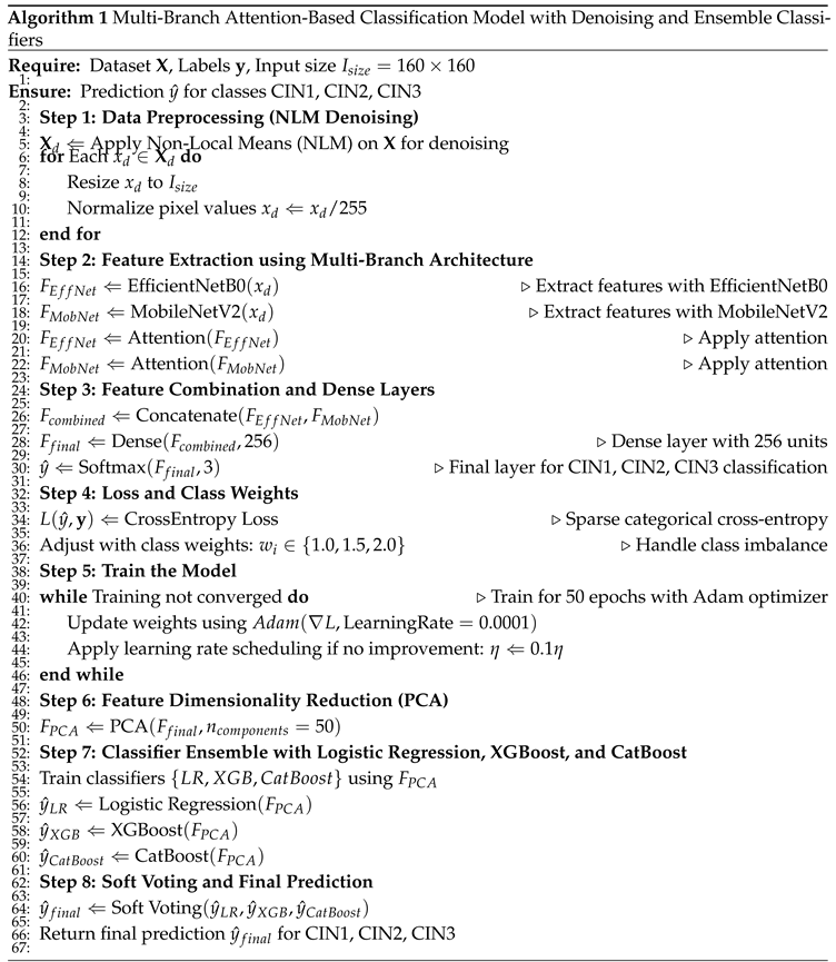
Based on Table 1 and Table 2, we were motivated to propose our model because of the following reasons: a. existing models were lacking lesion specific feature extraction; b. existing models relied on a single CNN for feature extraction that might miss to capture important features; c. either the use of only a linear classifier or the use of only a nonlinear classifier; d. no mechanism to handle class imbalance or to handle overfitting. Figure 1 is the work flow of the proposed architecture, which is divided into seven steps; a. preprocessing; b. using the multi-branch architecture of EfficientNetB0 and MobileNetV2 with an attention mechanism at the dense layer of each branch; c. the combined feature of this ensemble is provided with a mechanism to handle class imbalance; d. training; e. PCA is applied before the data is given to the classifiers; f. use of three classifiers, and each classifier is provided with hyperparameter fine tuning and K-fold cross validation; g. soft voting is applied to the output of the classifiers to prioritize the performance of the classifiers. As an output of this architecture, we are plotting the AUC curve showing the multi class classification as CIN1 indicating mild dysplasia, CIN2 depicting moderate dysplasia, and CIN3 refers to severe dysplasia or carcinoma in situ, all stages of abnormal cervical cell growth with increasing severity.

3.1. Data Preprocessing

The images are acquired from International Agency for Research on Cancer [24]. We were given 913 HPV positive data of CIN1, CIN2 and CIN3 captured in three different solutions. In order to get a maximum classification accuracy with respect to our proposed architecture, we have carried out image denoising and data augmentation that are described in the subsequent sections.

3.1.1. Image Denoising

It is to be noted that the colposcopy images are captured in varying lightning conditions that affects the images with noise. Moreover, moistening the cervix area before performing colposcopy also leads to specular spots that degrades the image quality. This has made us to denoise the images using Non-Local Means (NLM) algorithm, improving clarity while preserving details.

Mathematical Basis

v ( i ) = 1 Z ( i ) j Ω w ( i , j ) u ( j )
where v ( i ) denotes the denoised value of pixel i, u ( j ) represents the intensity of pixel j, w ( i , j ) indicates the similarity weight between pixels i and j, and Z ( i ) is the normalization factor.

3.1.2. Data Augmentation

We have carried out image augmentation on 913 images of CIN1, CIN2 and CIN3 from the sources. As our proposed architecture is ideal for a large dataset, we applied image augmentation technique so tha we could get a total of 6000 images.

3.2. Ensemble of Two CNNs with Attention Mechanism

The multi-branch architecture combines EfficientNetB0 and MobileNetV2 (EfficientNetB0 is chosen for its balance between accuracy and efficiency, while MobileNetV2 is ideal for low-computation environments, making their combination optimal for achieving both high performance and resource efficiency which is the target of this study.) as feature extractors, allowing for the extraction of diverse feature sets from the same image, enhancing the model’s representational power. The last 30 layers of both models are unfrozen for fine-tuning to capture lesion-specific features. An attention mechanism is applied to each branch to focus on important regions in the image, improving class discrimination between CIN1, CIN2, and CIN3. The feature outputs from both models are concatenated to provide a richer feature set for classification. A dense layer followed by a softmax layer outputs probabilities for classifying images into CIN1, CIN2, or CIN3.

Mathematical Basis

L ( θ ) = 1 N i = 1 N c = 1 C y i c log y ^ i c + λ j = 1 M | | W EffNet , j | | 2 2 + k = 1 M | | W MobileNet , k | | 2 2
Explanation: L ( θ ) is the total loss function. The first term, 1 N i = 1 N c = 1 C y i c log y ^ i c , represents the categorical cross-entropy loss, where N is the number of data samples, C is the number of classes (e.g., CIN1, CIN2, CIN3), y i c is the ground truth label for sample i and class c, and y ^ i c is the predicted probability for sample i and class c. The second term, λ j = 1 M | | W EffNet , j | | 2 2 + k = 1 M | | W MobileNet , k | | 2 2 , represents the L2 regularization (or weight decay) applied to the weights of EfficientNetB0 and MobileNetV2. In this, λ is the regularization coefficient, W EffNet , j refers to the weights of the j-th layer of EfficientNetB0, W MobileNet , k refers to the weights of the k-th layer of MobileNetV2, and | | W | | 2 2 is the L2 norm (squared) of the weights, which penalizes large weight values to prevent overfitting.
A ( F ) = σ 1 H × W i = 1 H j = 1 W F i j
Explanation: A ( F ) represents the attention mechanism applied to the feature map F. The term 1 H × W i = 1 H j = 1 W F i j computes the average of the feature map activations across the spatial dimensions, where H and W are the height and width of the feature map, respectively, and F i j is the activation at position ( i , j ) . The function σ ( · ) is the sigmoid activation function, which scales the attention score to a value between 0 and 1, indicating the importance of different regions in the feature map.
F = Concat ( A ( F EffNet ( x ) ) , A ( F MobileNet ( x ) ) )
where F is the concatenated feature map obtained by applying attention mechanisms A to both F EffNet ( x ) and F MobileNet ( x ) , combining their strengths into a single, enriched feature set.
y ^ = Softmax ( W · F + b )
where y ^ represents the final model output, where the softmax function converts the weighted feature set W · F + b into class probabilities for CIN1, CIN2, and CIN3.

3.3. Class Imbalance Handling, Learning Rate Scheduling, Dimensionality Reduction, and Multi Class Classification

Class Weights for Imbalance Handling

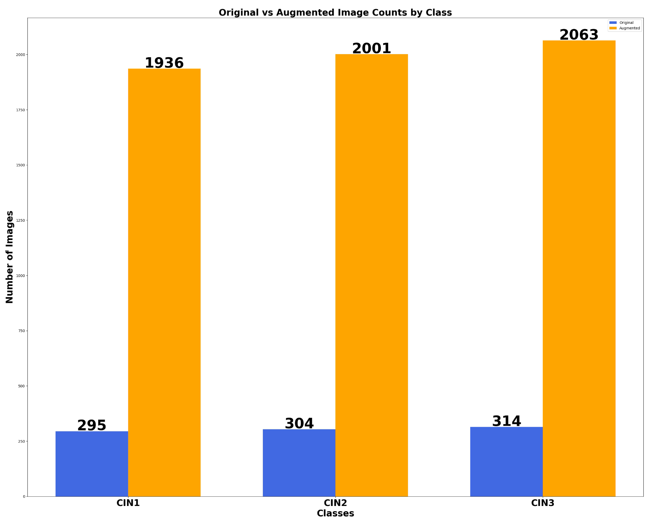
To handle class imbalance, as in the case of our dataset 295 images of CIN1, 304 images of CIN2, and 314 images of CIN3, class weights are applied to ensure that underrepresented classes are given more importance during training, preventing bias toward the majority class.
L weighted ( θ ) = 1 N i = 1 N w y i c = 1 C y i c log y ^ i c
Explanation: L weighted ( θ ) is the weighted loss function. The term w y i is the class weight corresponding to the true class y i , ensuring that the loss for underrepresented classes is increased to balance the dataset.

Learning Rate Scheduling

When the validation loss reaches a plateau, a learning rate scheduler like ReduceLROnPlateau lowers the learning rate to encourage steady convergence and avoid overfitting. In case of our proposed architecture, the learning rate scheduling was used after 80th epoch as there was no improvement in validation accuracy.
η t + 1 = η t · γ
Explanation: η t + 1 is the updated learning rate, where η t is the current learning rate and γ is a decay factor (typically 0 < γ < 1 ) applied when the validation loss plateaus.

PCA for Dimensionality Reduction

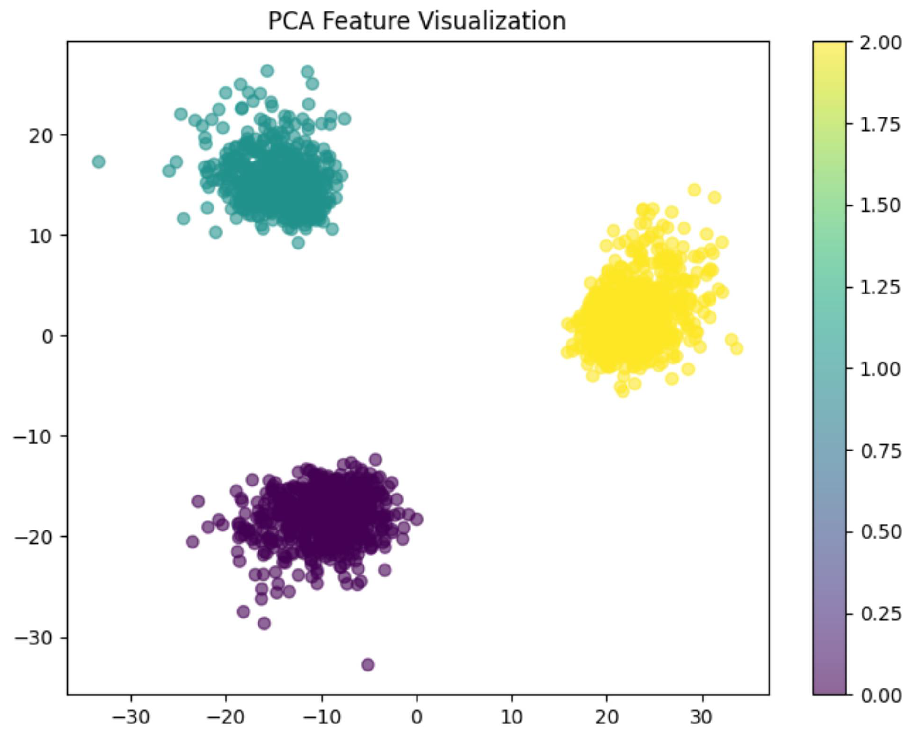
The extracted feature shapes (2233, 256) and (559, 256) from two CNNs, were reduced by PCA to 2D, enabling visualization of the data in two dimensions. This dimensionality reduction is a benefit to the classifiers like Logistic Regression, XGBoost, and CatBoost for reducing computational complexity.
Z = X W PCA
Explanation: Z is the reduced feature set after applying PCA, where X is the original feature matrix and W PCA is the matrix of principal components.

Logistic Regression, XGBoost, and CatBoost

Logistic Regression is used for linear classification, XGBoost captures complex patterns via gradient boosting, and CatBoost is effective in handling categorical data with minimal preprocessing. XGBoost and CatBoost is used in our architecture for non linear classification. Combining these in a soft-voting ensemble ensures more robust classification.
y ^ = σ ( W T Z + b )
Explanation: y ^ represents the predicted probability, with Z as the input feature vector after applying PCA, W as the weight vector, and b as the bias term. The sigmoid function, σ ( · ) , is used in logistic regression for binary or multi-class classification.
L ( θ ) = i = 1 N l ( y i , y ^ i ) + k = 1 T Ω ( f k )
Explanation: The XGBoost loss function consists of two parts: the first term is the loss l ( y i , y ^ i ) between the true label y i and the predicted label y ^ i , and the second term Ω ( f k ) is the regularization for tree complexity, controlling the depth and structure of decision trees.
L CatBoost ( θ ) = i = 1 N y i log ( y ^ i ) ( 1 y i ) log ( 1 y ^ i ) + λ j = 1 M | | W j | | 2 2
Explanation: The CatBoost loss function includes a standard binary cross-entropy loss with regularization. λ j = 1 M | | W j | | 2 2 is the L2 regularization term, preventing overfitting by penalizing large weights.

Hyperparameter fine tuning and K-Fold cross validation

This study involves hyperparameter tuning, model evaluation, and class-wise performance measurement using K-fold cross-validation on three classifiers: Logistic Regression, XGBoost, and CatBoost. Each classifier is optimized to improve accuracy and class-specific performance, targeting the multi-class classification problem with CIN grades (CIN1, CIN2, CIN3).

1. Hyperparameter Tuning with Grid Search

The hyperparameter tuning for each classifier is performed using GridSearchCV, optimizing for accuracy across a 5-fold cross-validation.
Best Model = arg max θ 1 K k = 1 K Accuracy y ^ train k , f ( X train k ; θ )
Explanation: In Equation (12), Best Model represents the model with the best hyperparameter set θ . Here, K denotes the number of folds in cross-validation (with K = 5 in this study). The term y ^ train k refers to the true labels for the training fold k, while f ( X train k ; θ ) represents the model’s predictions on fold k with hyperparameters θ . Finally, Accuracy is a measure that computes the fraction of correct predictions.
Purpose: Hyperparameter tuning optimizes each model to achieve the highest accuracy by finding the best set of hyperparameters for Logistic Regression, XGBoost, and CatBoost.

2. Class-wise Evaluation with K-fold Cross-Validation

After tuning, each model is evaluated using 5-fold cross-validation, calculating class-specific Precision, Recall, and F1 scores for each CIN grade. This ensures robust performance across classes.
Metrics Class = 1 K k = 1 K Precision Class , Recall Class , F 1 Class k
Explanation: In this context, Metrics Class represents a vector containing Precision, Recall, and F1 score values for each class. Specifically, Precision Class denotes the precision metric for the selected class, Recall Class refers to the recall for that class, and F 1 Class is the F1 score for the class, which is calculated as:
F 1 Class = 2 × Precision Class × Recall Class Precision Class + Recall Class
Purpose: This evaluation step ensures that each model performs well across different classes (CIN1, CIN2, CIN3) by measuring their specific Precision, Recall, and F1 scores, which are crucial for balanced multi-class classification performance.

Soft-Voting Ensemble

y ^ ensemble = 1 3 y ^ LR + y ^ XGBoost + y ^ CatBoost
Explanation: y ^ ensemble represents the final output from the soft-voting ensemble, where y ^ LR , y ^ XGBoost , and y ^ CatBoost are the predictions from Logistic Regression, XGBoost, and CatBoost, respectively. The final prediction is the average of the predicted probabilities from all classifiers.

4. Algorithm

Preprints 138279 i001

5. Implementation

5.1. Experimental Setup

All the experiments are carried out in Intel(R) Core(TM) i5-1035G1 CPU @ 1.00GHz, 1.19 GHz, 16GB RAM, 1.4 TB HD and windows 11, 64 bit operating system configuration. To execute our proposed architecture we have used Colab Pro in TPU V2-8 as a hardware accelerator that has provided us with 334.5 GB of high RAM, 225.33 GB of disk, and 500 GB of computational units. All the experiments are conducted for 100 epochs with a test-train split of 80:20.

5.2. Performance Metrics

The performance of the proposed algorithm will be evaluated to ensure model efficiency, with the choice of evaluation criteria tailored to the dataset and selected metrics. In this study, the primary dimensional metric is the number of classes. Additionally, we are assessing other performance metrics to analyze the impact of increasing class numbers. Specifically, we will examine accuracy, specificity, and sensitivity, aligning with metrics commonly used in prior studies for algorithm performance measurement [25]. Table 3 provides an overview of all the metrices used in this study.

5.3. Dataset

We have received a total of 918 images of CIN1, CIN2 and CIN3 positive images from International Agency for Research on Cancer [24] captured in three different solutions; Lugol’s iodine, Acetic acid and normal saline. We have removed the images captured using green filter for our study which made us to have a total of 913 images. We are referring this data as our primary dataset. We have denoised and augmented this dataset. Apart from this we have also used a secondary dataset, the Malhari dataset [50] containing a total of 2,790 images.

5.3.1. Primary Dataset

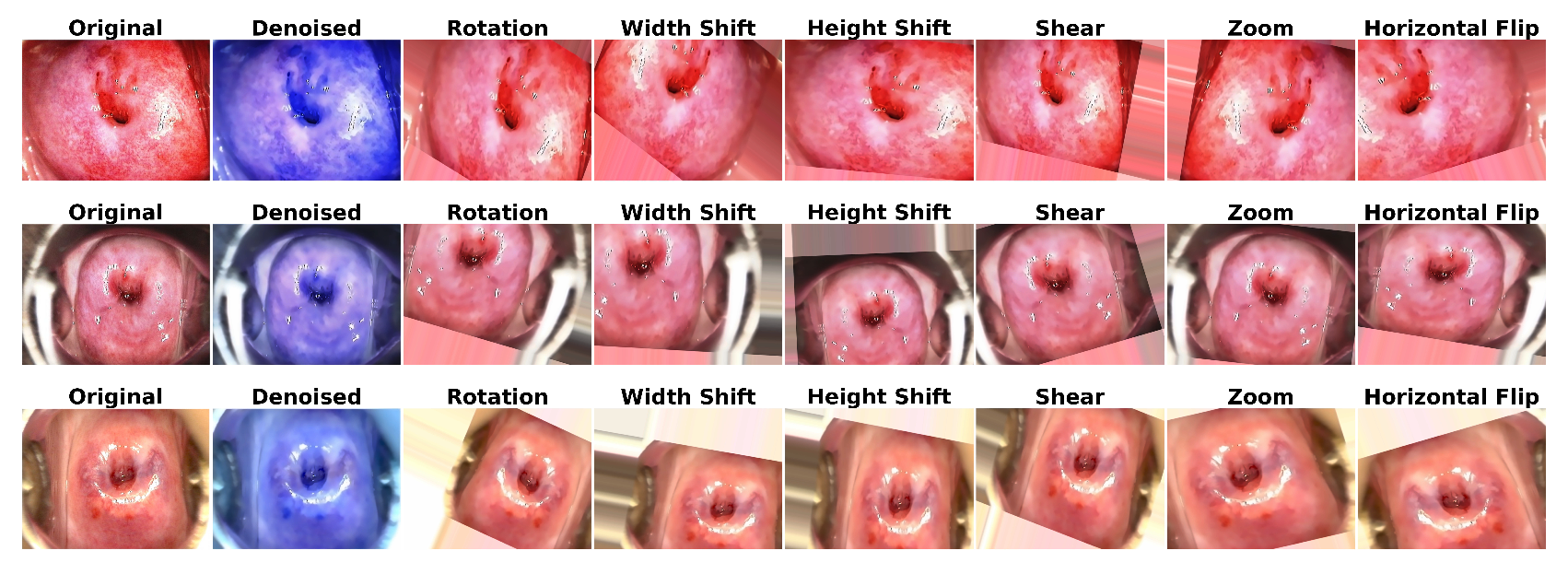
A total of 913 images containing 295 CIN1 images, 304 CIN2 images, and 314 CIN3 images were augmented to 1936 for CIN1, 2001 for CIN2 and 2063 for CIN3. We have used a separate directory to store 6,000 augmented images. We have used ImageDataGenerator for augmentation, implementing rotation by 30 degrees, width-shift range=0.2 and height-shift range=0.2, shear range=0.2, zoom-range=0.2, horizontal flip=True, and fill mode=’nearest’. Figure 3 is the class distribution of original and augmented images. We have used this dataset after denoising.

5.3.2. Distribution of Images of the Primary Dataset in Lugol’s Iodine, Acetic Acid and Normal Saline

Table 4 shows the distribution of images class-wise of the primary dataset captured in three different solutions. We have used this dataset without denoising and stored the 6,000 augmented images in a separate directory. We implemented rotation by 30 degrees, width-shift range=0.2, height-shift range=0.2, shear range=0.2, zoom-range=0.2, horizontal flip=True, and fill mode=’nearest’ using ImageDataGenerator for augmentation.

5.3.3. Secondary Dataset

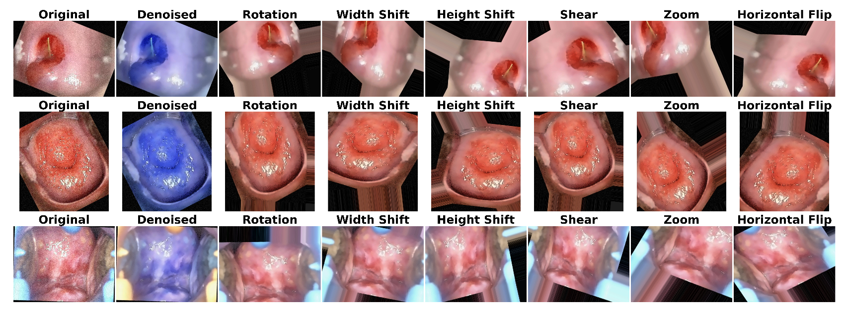
Table 5 shows the distribution of images class-wise of the secondary dataset. We implemented rotation by 30 degrees, width-shift range=0.2, height-shift range=0.2, shear range=0.2, zoom-range=0.2, horizontal flip=True, and fill mode=’nearest’ using ImageDataGenerator for augmentation. We have stored 6,000 enhanced denoised photos in a different directory.

6. Results and Discussions

6.1. Results of Data Preprocessing and Image Augmentation

This study utilizes two datasets: the primary dataset is sourced from IARC [24], and the secondary dataset, referred to as Malhari, is from Kaggle [50]. The images in the primary dataset have a resolution of 800 × 600 pixels, while those in the secondary dataset are sized at 640 × 480 pixels. Both datasets consist of images in JPG format, maintaining a 4:3 aspect ratio. For our proposed architecture, each dataset was augmented to contain 6,000 images, and denoising was applied using the NLM algorithm. Due to the use of computationally intensive CNNs for feature extraction, the image size for both datasets was reduced to 160 × 160 pixels. Figure 3 and Figure 4 illustrate sample images from both datasets after applying denoising and augmentation. The first row represents CIN1, the second row shows CIN2, and the third row displays CIN3.

6.2. Results of Model Training on Primary Dataset from IARC

As our model is divided into parts, starting with preprocessing and ending with the multiclass classification, in the susequent sections we are providing the result and its analysis of each part of the architecture.

6.2.1. Training Results and Analysis

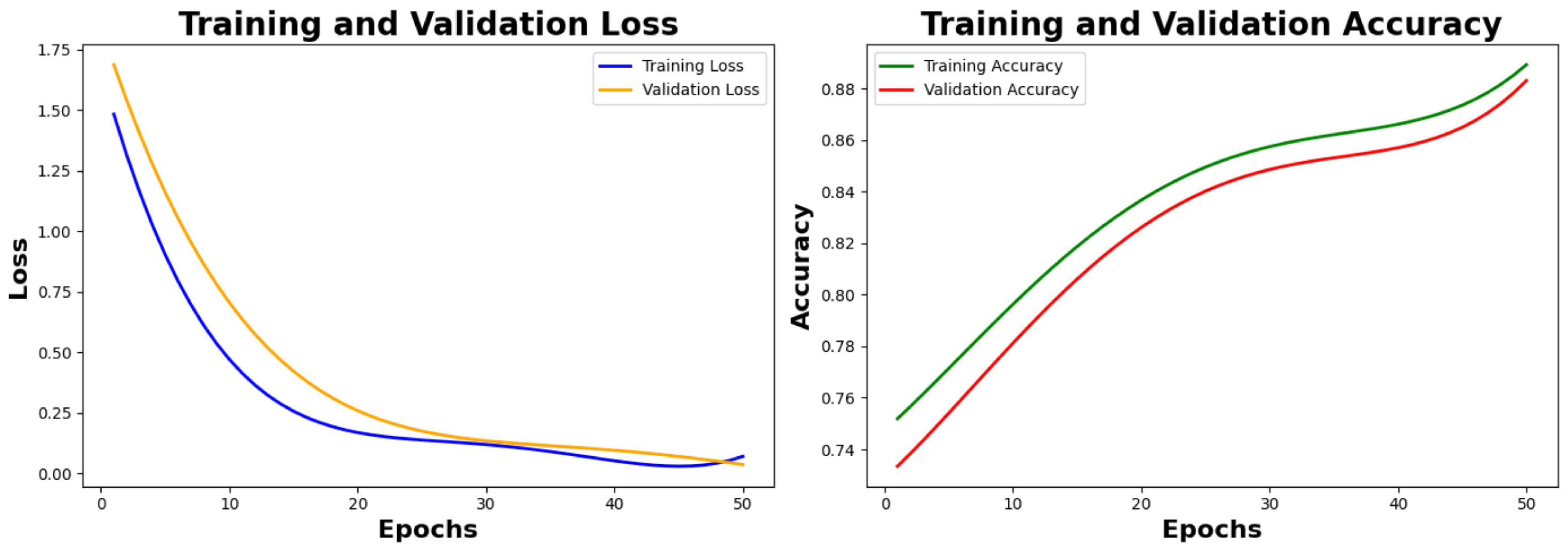
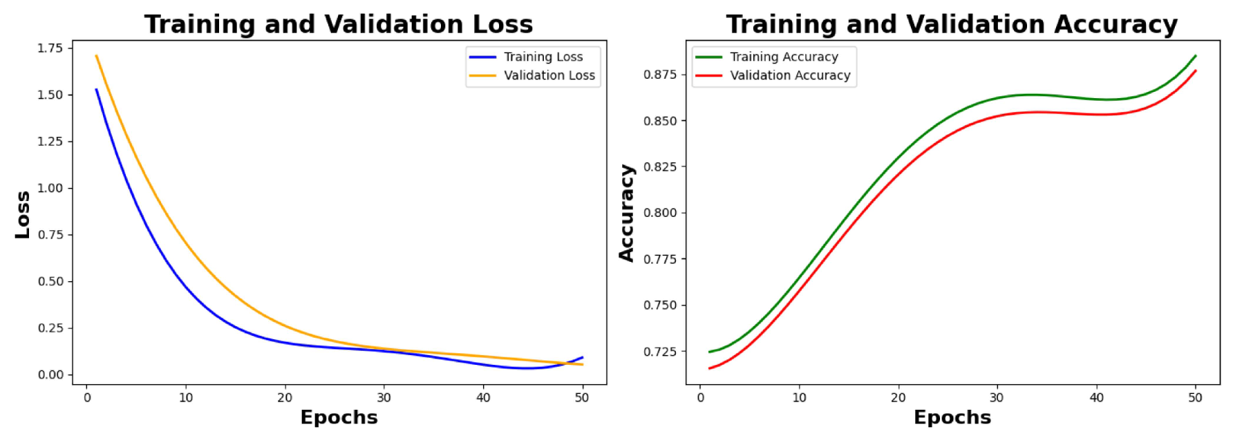
The model is primarily implemented on 913 denoised, augmented images (6,000) with a train-test split of 80:20. So, there are 4800 training samples and 1200 test samples. The model was executed for 100 epochs with a batch size of 32 epochs and 150 iterations per epoch. The validation loss was observed to be constant after 80th epoch, so ReduceLROnPlateau was used to reduce the learning rate till 100th epoch. The training accuracy at the training phase after 100th epoch was obtained as 97.85% and the validation accuracy at the training phase after 100th epoch was 97.33%. For each epoch, we have noted the performance metrics: recall, precision, F1, validation loss, validation accuracy, training loss, and training accuracy. Figure 5 show the loss and accuracy trends for the first 50 epochs. Table 6 presents the precision, recall, and F1 scores obtained at the final 100th epoch, prior to feeding the features into the classifier. .

Analysis

The graph 5 shows the trend of training loss, validation loss, training accuracy, and validation accuracy. We are showing this trend for the first 50 epochs. The training loss graph starts from 1.4176 and converges to 0.0416. The validation loss graph starts at 1.6548 and converges to 0.0508. The training accuracy at 50th epoch is 88.18% and the validation accuracy at the 50th epoch is 87.69%. Both the training loss and validation loss graphs are smooth and show a downward trend, showing that the model is able to generalize well and there is no overfitting or underfitting. Considering the acuuracy graphs, there is an upward trend of both graphs depicting that the models are able to classify the training samples with greater precision over time. There is a slight gap between the training and the validation accuracy graph hinting there might be a mild overfitting as the model continues to specialize on the training data. However, the close alignment between training and validation accuracy is an encouraging sign of the model’s generalization capabilities.

6.2.2. Feature Extraction, PCA, Hyperparameter Fine Tuning and K-Fold Cross Validation Results and Analysis

The output we got in this phase shows that 2,233 training samples and 559 validation samples were passed through the feature extraction model, resulting in feature vectors of shape (256). Hyperparameter tuning was performed for three models: Logistic Regression with 3 hyperparameter combinations, XGBoost with 4 combinations, and CatBoost with 8 combinations. For cross-validation, Logistic Regression performed 15 fits (3 candidates x 5 folds), XGBoost performed 20 fits, and CatBoost performed 40 fits using 5-fold cross-validation. PCA is being used to reduce the dimensionality of the extracted features. After extracting 256-dimensional feature vectors from the deep learning model (EfficientNet + MobileNetV2), PCA is applied to reduce the number of features to 50. Hyperparameter tuning is applied to the three machine learning classifiers: Logistic Regression, XGBoost, and CatBoost, using GridSearchCV to find the optimal combination of hyperparameters for each model. Logistic Regression classifier is initialized with a maximum of 1000 iteration, meaning it will continue to optimize until convergence or 1000 iterations. In case of XGBoost, a set of hyperparameters is defined including the number of estimators (50 and 100), tree depth (3 and 5), and learning rate of 0.1. The grid defined for CatBoost, with the number of iterations (100 and 200), tree depth (3 and 5), and learning rate of 0.01 and 0.1.
For each classifier, GridSearchCV is used to perform an exhaustive search over the hyperparameter grid. The search is performed using 5-fold cross-validation (cv=5), meaning the data is split into 5 parts, with 4 used for training and 1 for validation in each iteration. The search is based on maximizing accuracy (scoring=’accuracy’). The verbose=1 parameter ensures that details of the training process are printed during the search. After fitting the models, the best hyperparameter combination for each classifier is selected using best-estimator. This gives us the most optimal Logistic Regression, XGBoost, and CatBoost models based on the cross-validation search.
In soft voting, the predicted probabilities from each model are averaged, and the class with the highest average probability is selected as the final prediction. This tends to work better for classifiers that output reliable probabilities. StratifiedKFold initializes a 5-fold cross-validation strategy that ensures each fold maintains the relative class proportions.

Analysis

Table 7 compares the performance of three classifiers—Logistic Regression, XGBoost, and CatBoost—after hyperparameter tuning across five folds of cross-validation. The metrics include accuracy, precision, recall, and F1-score for each classifier on each fold. In the case of LR, the accuracy across all folds is very consistent, ranging from 0.9731 to 0.9821 with high precision, recall, and F1-scores. Fold 3 and Fold 5 show the best performance with an accuracy of 0.9821 and an F1-score of 0.9822, suggesting consistent model reliability across folds. In the case of XGBoost, shows slightly higher accuracy compared to LR, with accuracies ranging from 0.9687 to 0.9843. Precision, recall, and F1-scores are also high, particularly in Fold 1 (F1: 0.9843), but there is slight variation across the other folds. Fold 3 shows the lowest accuracy (0.9687), but overall, XGBoost maintains strong performance across all folds. In the case of CatBoost, shows the highest performance across the classifiers, with accuracy values ranging from 0.9687 to 0.9905. It demonstrates excellent precision, recall, and F1-scores, achieving high values across all folds. CatBoost, especially in Fold 1 and Fold 5, shows superior consistency, making it the best-performing classifier in this comparison.
Table 8 shows the validation accuracy, precision, recall and F1 of each classifier class wise. The table also shows the values of these metrics after a soft voting is applied. All classifiers demonstrate excellent performance, with Precision, Recall, and F1-Score values close to 1.000, reflecting high accuracy in classification. Logistic Regression achieves slightly lower values than the other models, particularly in Recall and F1-Score, indicating it may struggle slightly with a few mis-classifications. XGBoost performs similarly to CatBoost with high scores across all metrics but has a slightly lower Precision for CIN3. CatBoost shows perfect classification in nearly all metrics and classes, matching the Ensemble model in performance. Ensemble Voting Classifier delivers the highest overall performance, with near-perfect Precision, Recall, and F1-Score, reflecting the benefit of combining multiple classifiers.

6.2.3. PCA Visualization, AUC Graph and Confusion Matrix Plot

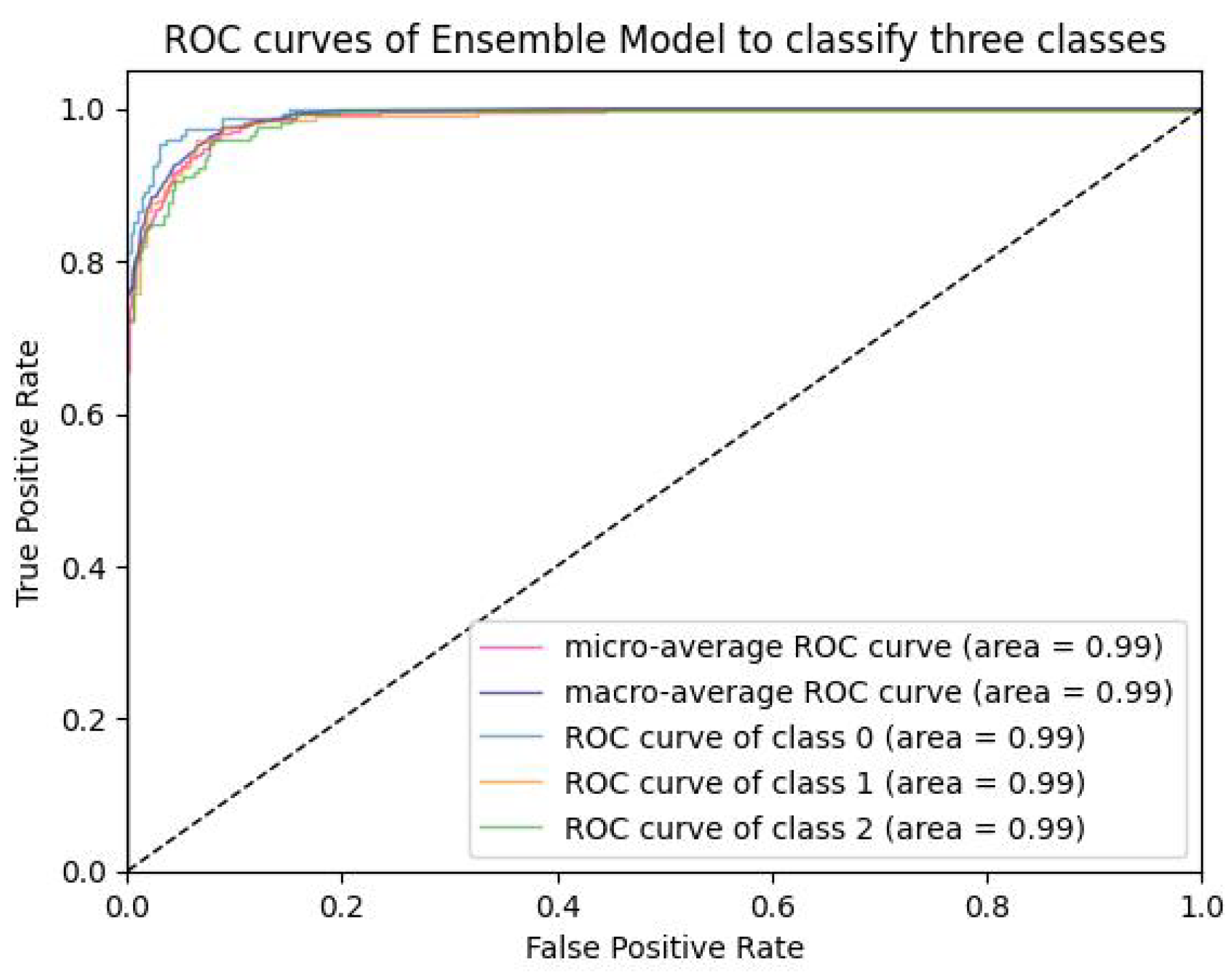
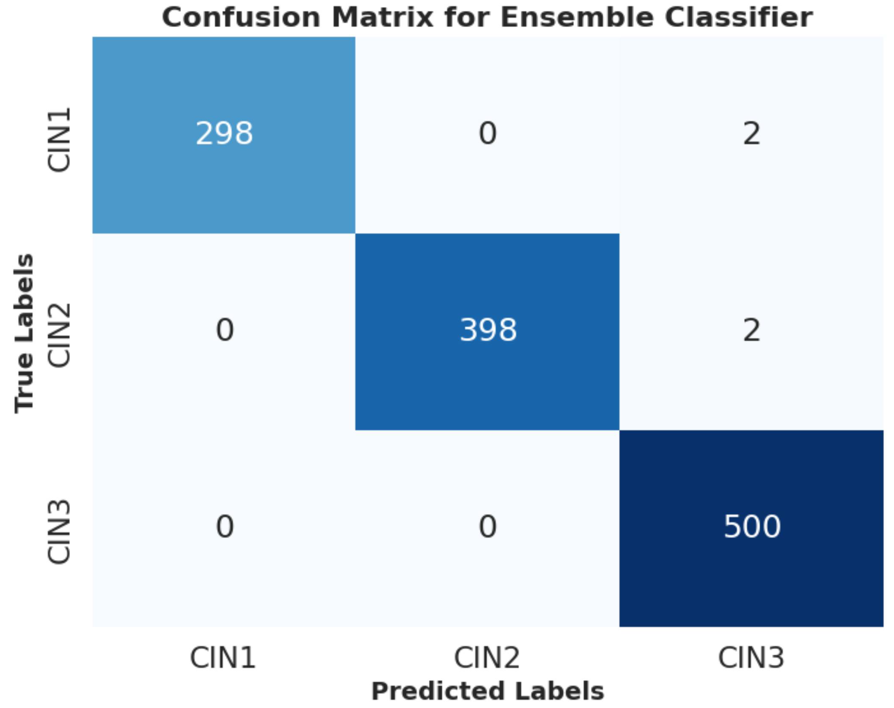
Figure 6 and Figure 7 shows the plot of PCA visualization and AUC curve of the three class classification by the ensemble model. Figure 8 is the confusion matrix plot of the ensemble voting system.

Analysis

From Figure 6, the three distinct clusters represent the three CIN classes, showing clear separation between the classes, which is crucial for effective classification. This indicates that the extracted features from the model are well-separated and hold meaningful information for distinguishing between the classes. In Figure 7, the AUC curves for the multi-class classification show high classification performance, with AUC values close to 1.0 for all three classes (CIN1, CIN2, CIN3). The micro- and macro-average ROC curves also approach the upper left corner of the plot, further confirming the strong discriminative ability of the model. This indicates that the ensemble model can effectively classify the different CIN grades with high accuracy, precision, and recall across the classes. Figure 8 shows the confusion matrix for the ensemble classifier shows near-perfect classification performance across all three classes (CIN1, CIN2, and CIN3), with minimal misclassifications. Out of 300 samples in CIN1, 298 were correctly classified, and 2 were misclassified as false negatives (classified as CIN3). There are no false positives for CIN1. Out of 400 samples in CIN2, 398 were correctly classified, and 2 were misclassified as false negatives (classified as CIN3). There are no false positives for CIN2. All 500 samples in CIN3 were correctly classified with no misclassifications.

6.3. Test Result of the Model on Primary Denoised IARC Dataset

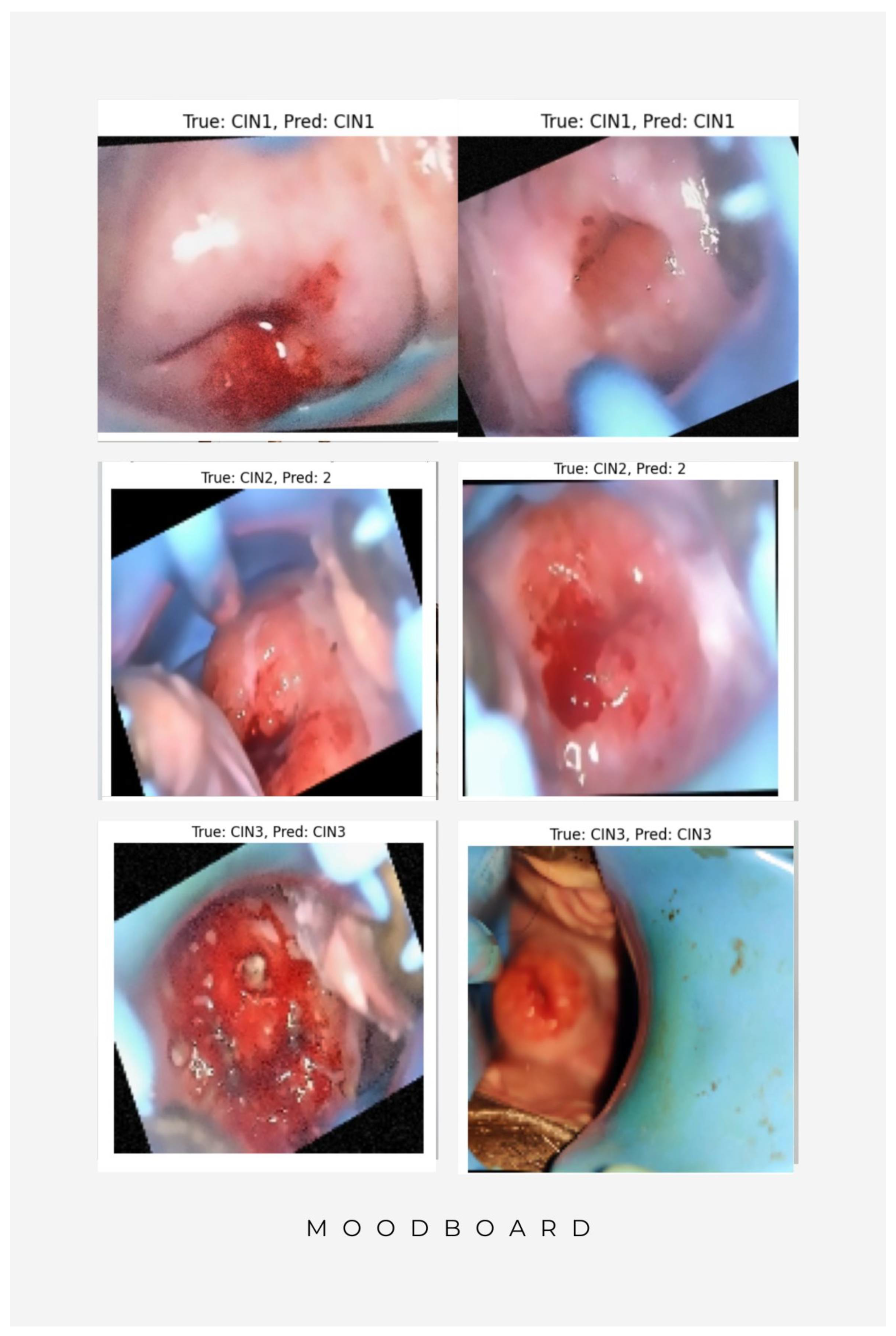
This section deals with a test dataset of 1000 images on which we have tested our proposed algorithm for predicting the correct labels with respect to true labels. Few of these images are validated by a senior oncologist. We are providing a sample of images of three classes that our model predicted correctly. Figure 9 shows some sample images of three classes as seen as true and predicted images.

6.4. Result Analysis of the Primary Noisy Dataset Separated by Solutions and Denoised Secondary Dataset

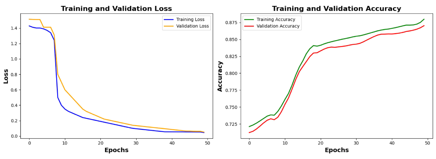
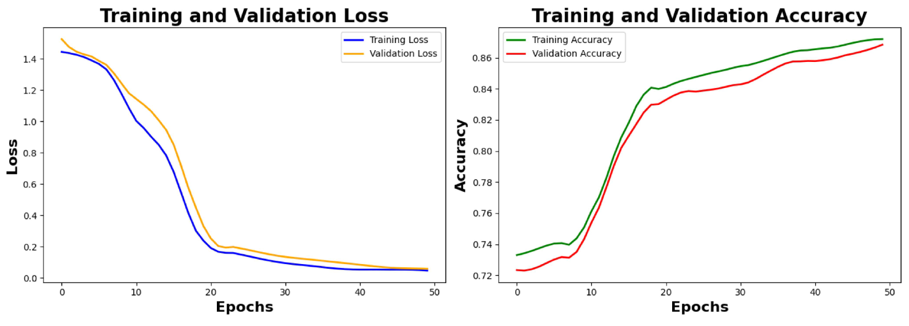
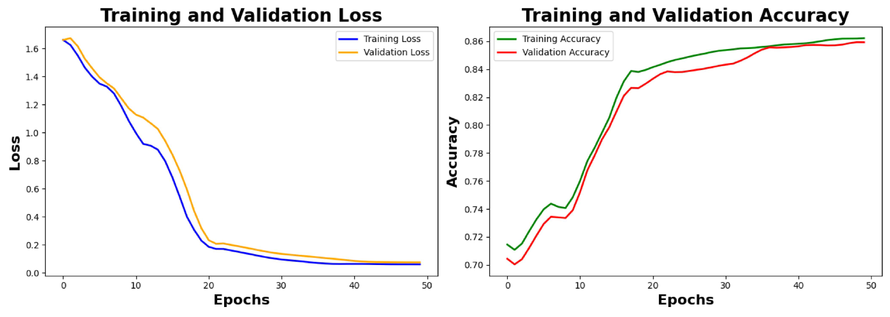
This section does an analysis of the model’s performance on different datasets. Figure 10, Figure 11, Figure 12 depicts the trends of the both the loss and both the accuracy of the model on the primary dataset, where the images are separated as per their capturing in three different solutions; Lugol’s iodine, acetic acid and normal saline. These images are not denoised to test the behavior of the model on denoised images. Figure 13 shows the trends of both the losses and the accuracies of the model on a secondary dataset.

Analysis of Loss graphs and accuracy graphs

In the case of Figure 10, the training loss starts from 1.4276 and converges to 0.0452 at the 50th epoch. The validation loss starts from 1.5148 and converges to 0.0516 in the 50th epoch. Both the graphs are smooth, and the trend of the loss is decreasing. Considering the trends of the accuracies, the rise is upward, there is a slight overlap suggesting the data is noisy and there might be overfitting. Though Lugol’s iodine is a proper solution to use for colposcopy, the training accuracy reaches to 88.11% and the validation accuracy reaches to 87.14% for the 50th epoch.
Figure 11 is the trend of loss and accuracy of the dataset using acetic acid solution. The training loss starts at 1.4484 and converges to 0.0469 at the 50th epoch. The validation loss starts at 1.5148 and converges to 0.0588 at the 50th epoch. There is a slight fluctuation in both the graphs as the dataset is noisy and the solution used is acetic acid that is not as appropriate as Lugol’s iodine for colposcopy. Both the graphs shows a correct trend but the accuracy value of the training is 87.21% and the validation accuracy is 86.94%, lower than the accuracies of Lugol’s iodine.
Considering Figure 12, though both the graphs show correct trends for the first 50th epoch, the training accuracy is 86.21% and the validation accuracy is 85.94% that is way behind the accuracies reached for the images in Lugol’s iodine and acetic acid solutions. There is fluctuation in both the graphs but from the trend of the graphs it is clear that both of them tries to generalize well on unseen data.
Figure 13 is the graph for the secondary dataset. Both the graphs shows correct trend. There is a smooth decline in the loss graph indicating there is no overfitting or underfitting. There is a fluctuation in the accuracy graph, but as per the trend, the model is performs more effectively on denoised data, likely due to reduced interference from noise, leading to better generalization.

Analysis of performance metrics of noisy dataset in three solutions and the secondary dataset

Table 9 compares precision, recall, and F1 scores across four different datasets (Lugol’s Iodine, Acetic Acid, Normal Saline, and Malhari) for classifying CIN grades (CIN1, CIN2, and CIN3). The Malhari dataset being denoised shows the highest and most consistent performance across all CIN grades, with precision, recall, and F1 all at 0.98. Across all datasets (noisy or denoised), CIN3 tends to have slightly higher precision and recall compared to CIN1 and CIN2, suggesting the model is slightly better at identifying this grade. The Normal Saline dataset has slightly lower metrics (0.95-0.96) for all CIN grades, indicating a potential challenge in classification with this dataset compared to others. In summary, the Malhari dataset provides the best performance, while Normal Saline shows the lowest scores, especially in recall for CIN2.

6.5. Result Analysis of Recent Existing Approaches, Baseline Architecture and Variation of the Proposed Model

Table 10 shows a comparison of selected approaches from Table 1, some baseline architecture with variation of the proposed architecture. Based on the complexity of the model [25,26,27], we have modified the algorithms by changing their batch size (keeping structure the same) so that we could implement them on our 6,000 denoised primary dataset. All the other models were executed for 100 epochs on our primary dataset. We have used the same system configuration as mentioned in Section 5.1.

Analysis

[25] : We have executed this algorithm by starting the learning rate at 0.01. The model currently uses 3 × 3 convolutions across layers; we have reduced the number of filters in the first few layers without compromising on the accuracy. As we have executed in TPU V2-8, we have used a slightly lower dropout rate since TPUs generally converge faster and may need less dropout. As TPU can handle larger batch sizes, we have used 128 batch size in this case and made the model run for 100 epochs. The validation accuracy obtained in this case is lower than the proposed architecture, as our architecture combines feature extraction strengths from multiple CNNs, an attention mechanism, and diverse classifiers in a stacked approach.
[26] : We have executed this algorithm by starting the learning rate at 0.01. As TPU can handle larger batch sizes, we have used 128 batch size in this case and made the model run for 100 epochs. We have converted the first three stages (CNN-KNN, CNN-RF, and CNN-SVM) into sequential blocks, ensuring they do not run concurrently. After processing each stage, we saved the intermediary predictions for the next stage. For the MLP layer in Stage 4 we have made it TPU-optimized by using Keras tf.keras.layers.Dense layers instead of custom implementations. The validation accuracy of this architecture is lesser than the proposed architecture, when implemented on 6,000 colposcopy images with a batch size of 128 and 100 epochs, as though this model may generalize well, the lack of a refined focus mechanism, like attention, could limit its performance on complex visual data like colposcopy images.
[27] : This architecture uses different strategies for validating the performance of the model; inner to outer and outer to inner, checks with different values of K and finally selects K=100, validates the performance of the model using single class data split and multi class data split. We have directly implemented this research work, considering the value of K=100 for KNN, using stratified K-fold cross validation, using multi class data split and using one learning strategy(inner to outer), got a validation accuracy lower than our proposed method. If we would have gone with the published architecture of this research, the architecture would have been computationally intensive due to the extensive cross-validation and feature integration steps. It would likely perform well on TPU but may have a longer runtime due to the layer complexity. We have modified the model to reduce its computational complexity so that it matches with our proposed architecture, but yielded a lower accuracy than our architecture.
The reason for lower validation accuracy by these models are; ResNet50 is a solid choice for image classification but lacks efficiency in handling fine-grained details often needed for medical images, DenseNet121 has a densely connected structure that helps in capturing more detailed information, but as a single model, it lacks the robustness provided by an ensemble approach, EfficientNetB0 is optimized for efficient scaling but is limited as a standalone model for complex multi class medical classification tasks, MobileNetV2 acks the attention and ensemble mechanisms needed to effectively capture critical and nuanced details in the images, Combining EfficientNetB0 and MobileNetV2 adds diversity to feature extraction, but without an attention mechanism, it lacks the ability to highlight relevant regions in the images, EffB0 + MobV2 (with attention), is the closest in structure to the proposed architecture but lacks the comprehensive multi-level feature handling and advanced ensemble and voting mechanisms seen in the proposed model.

7. Conclusions

This study introduces a multi-branched ensemble architecture enhanced with an attention mechanism to improve the classification accuracy of colposcopy images. The model employs EfficientNetB0 and MobileNetV2 in separate branches, where each branch’s dense layer incorporates an attention mechanism to capture critical lesion features. The extracted features from each branch are then combined and passed through an ensemble of three classifiers: Logistic Regression, XGBoost, and CatBoost. Logistic Regression acts as a meta-learner to mitigate overfitting, while XGBoost and CatBoost handle non-linear classification. Each of the classifiers output is hyperparameter fine tuned using Grid search technique and then validated using stratified K-fold cross-validation. The final multi-class classification is determined through soft voting across the outputs of all three classifiers. The proposed architecture is tested on a variety of datasets, and it’s result s also compared with existing technologies and baseline approaches.In all the cases, the proposed architecture has shown outstanding results.

Author Contributions

All the authors have equally contributed to this research.

Funding

This work is not funded from any external sources.

Data Availability Statement

The data which is used for this research was being gathered directly from IARC, WHO.

Conflicts of Interest

The authors have no conflicts of interests related to this research.

References

  1. Jacot-Guillarmod, M.; Balaya, V.; Mathis, J.; Hübner, M.; Grass, F.; Cavassini, M.; Sempoux, C.; Mathevet, P.; Pache, B. Women with Cervical High-Risk Human Papillomavirus: Be Aware of Your Anus! The ANGY Cross-Sectional Clinical Study. Cancers 2022, 14, 5096. [Google Scholar] [CrossRef] [PubMed]
  2. Bucchi, L.; Costa, S.; Mancini, S.; Baldacchini, F.; Giuliani, O.; Ravaioli, A.; Vattiato, R.; others. Clinical epidemiology of microinvasive cervical carcinoma in an Italian population targeted by a screening programme. Cancers 2022, 14, 2093. [Google Scholar] [CrossRef]
  3. Tantari, M.; Bogliolo, S.; Morotti, M.; Balaya, V.; Bouttitie, F.; Buenerd, A.; Magaud, L.; others. Lymph node involvement in early-stage cervical cancer: is lymphangiogenesis a risk factor? Results from the MICROCOL study. Cancers 2022, 14, 212. [Google Scholar] [CrossRef]
  4. Yao, K.; Huang, K.; Sun, J.; Hussain, A. PointNu-Net: Keypointassisted convolutional neural network for simultaneous multi-tissue histology nuclei segmentation and classification. IEEE Trans. Emerg. Topics Comput. Intell. 2024, 8, 802–813. [Google Scholar] [CrossRef]
  5. Ramzan, Z.; Hassan, M.A.; Asif, H.M.S.; Farooq, A. A machine learning-based self-risk assessment technique for cervical cancer. Current Bioinformatics 2021, 16, 315–332. [Google Scholar] [CrossRef]
  6. Parra, S.; Carranza, E.; Coole, J.; Hunt, B.; Smith, C.; Keahey, P.; Maza, M.; Schmeler, K.; Richards-Kortum, R. Development of low-cost point-of-care technologies for cervical cancer prevention based on a single-board computer. IEEE Journal of Translational Engineering in Health and Medicine 2020, 8, 1–10. [Google Scholar] [CrossRef] [PubMed]
  7. Shah, H.A.; Saeed, F.; Yun, S.; Park, J.H.; Paul, A.; Kang, J.M. A Robust Approach for Brain Tumor Detection in Magnetic Resonance Images Using Finetuned EfficientNet. IEEE Access 2022, 10, 65426–65438. [Google Scholar] [CrossRef]
  8. Si, L.; others. A Novel Coal-Gangue Recognition Method for Top Coal Caving Face Based on IALO-VMD and Improved MobileNetV2 Network. IEEE Transactions on Instrumentation and Measurement 2023, 72, 1–16, Art no. 2529216. [Google Scholar] [CrossRef]
  9. Ju, X.; Qian, J.; Chen, Z.; Zhao, C.; Qian, J. Mulr4FL: Effective Fault Localization of Evolution Software Based on Multivariate Logistic Regression Model. IEEE Access 2020, 8, 207858–207870. [Google Scholar] [CrossRef]
  10. Teng, W.; Wang, N.; Shi, H.; Liu, Y.; Wang, J. Classifier-Constrained Deep Adversarial Domain Adaptation for Cross-Domain Semisupervised Classification in Remote Sensing Images. IEEE Geoscience and Remote Sensing Letters 2020, 17, 789–793. [Google Scholar] [CrossRef]
  11. Prakash, A.; Thangaraj, J.; Roy, S.; Srivastav, S.; Mishra, J.K. Model-Aware XGBoost Method Towards Optimum Performance of Flexible Distributed Raman Amplifier. IEEE Photonics Journal 2023, 15, 1–10. [Google Scholar] [CrossRef]
  12. Tammina, S. Transfer learning using VGG-16 with deep convolutional neural network for classifying images. International Journal of Scientific and Research Publications (IJSRP) 2019, 9, 143–150. [Google Scholar] [CrossRef]
  13. Hasegawa, T.; Kondo, K. Easy Ensemble: Simple Deep Ensemble Learning for Sensor-Based Human Activity Recognition. IEEE Internet of Things Journal 2023, 10, 5506–5518. [Google Scholar] [CrossRef]
  14. Cui, X.; Wu, S.; Li, Q.; Chan, A.B.; Kuo, T.W.; Xue, C.J. Bits-Ensemble: Toward Light-Weight Robust Deep Ensemble by Bits-Sharing. IEEE Transactions on Computer-Aided Design of Integrated Circuits and Systems 2022, 41, 4397–4408. [Google Scholar] [CrossRef]
  15. Prakash, A.S.J.; Sriramya, P. Accuracy analysis for image classification and identification of nutritional values using convolutional neural networks in comparison with logistic regression model. Journal of Pharmaceutical Negative Results 2022, pp. 606–611.
  16. Das, P.; Pandey, V. Use of logistic regression in land-cover classification with moderate-resolution multispectral data. Journal of the Indian Society of Remote Sensing 2019, 47, 1443–1454. [Google Scholar] [CrossRef]
  17. Park, J.; Yang, H.; Roh, H.J.; Jung, W.; Jang, G.J. Encoder-weighted W-Net for unsupervised segmentation of cervix region in colposcopy images. Cancers 2022, 14, 3400. [Google Scholar] [CrossRef]
  18. Morales-Hernández, A.; Nieuwenhuyse, I.V.; Gonzalez, S.R. A survey on multi-objective hyperparameter optimization algorithms for machine learning. Artificial Intelligence Review 2023, 56, 8043–8093. [Google Scholar] [CrossRef]
  19. Ahmad, Z.; Li, J.; Mahmood, T. Adaptive hyperparameter fine-tuning for boosting the robustness and quality of the particle swarm optimization algorithm for non-linear RBF neural network modelling and its applications. Mathematics 2023, 11, 242. [Google Scholar] [CrossRef]
  20. Hua, Q.; Li, Y.; Zhang, J.; others. Convolutional neural networks with attention module and compression strategy based on second-order information. International Journal of Machine Learning and Cybernetics 2024, 15, 2619–2629. [Google Scholar] [CrossRef]
  21. Jiang, X.; Li, J.; Kan, Y.; Yu, T.; Chang, S.; Sha, X.; Zheng, H. MRI based radiomics approach with deep learning for prediction of vessel invasion in early-stage cervical cancer. IEEE/ACM Trans. Comput. Biol. Bioinf. 2020, 18, 995–1002. [Google Scholar] [CrossRef]
  22. Wang, C.; Zhang, J.; Liu, S. Medical Ultrasound Image Segmentation With Deep Learning Models. IEEE Access 2023, 11, 10158–10168. [Google Scholar] [CrossRef]
  23. Skouta, A.; Elmoufidi, A.; Jai-Andaloussi, S.; others. Deep learning for diabetic retinopathy assessments: a literature review. Multimedia Tools and Applications 2023, 82, 41701–41766. [Google Scholar] [CrossRef]
  24. International Agency for Research on Cancer. IARC: International Agency for Research on Cancer 2023.
  25. Youneszade, N.; Marjani, M.; Ray, S.K. A predictive model to detect cervical diseases using convolutional neural network algorithms and digital colposcopy images. IEEE Access 2023, 11, 59882–59898. [Google Scholar] [CrossRef]
  26. Zhang, S.; Chen, C.; Chen, F.; Li, M.; Yang, B.; Yan, Z.; Lv, X. Research on application of classification model based on stack generalization in staging of cervical tissue pathological images. IEEE Access 2021, 9, 48980–48991. [Google Scholar] [CrossRef]
  27. Luo, Y.M.; Zhang, T.; Li, P.; Liu, P.Z.; Sun, P.; Dong, B.; Ruan, G. MDFI: multi-CNN decision feature integration for diagnosis of cervical precancerous lesions. IEEE Access 2020, 8, 29616–29626. [Google Scholar] [CrossRef]
  28. Chen, P.; Liu, F.; Zhang, J.; Wang, B. MFEM-CIN: A Lightweight Architecture Combining CNN and Transformer for the Classification of Pre-Cancerous Lesions of the Cervix. IEEE Open J. Eng. Med. Biol. 2024, 5, 216–225. [Google Scholar] [CrossRef]
  29. Mathivanan, S.; Francis, D.; Srinivasan, S.; Khatavkar, V.; P, K.; Shah, M.A. Enhancing cervical cancer detection and robust classification through a fusion of deep learning models. Scientific Reports 2024, 14, 10812. [Google Scholar] [CrossRef]
  30. He, Y.; Liu, L.; Wang, J.; Zhao, N.; He, H. Colposcopic Image Segmentation Based on Feature Refinement and Attention. IEEE Access 2024, 12, 40856–40870. [Google Scholar] [CrossRef]
  31. Bappi, J.O.; Rony, M.A.T.; Islam, M.S.; Alshathri, S.; El-Shafai, W. A Novel Deep Learning Approach for Accurate Cancer Type and Subtype Identification. IEEE Access 2024, 12, 94116–94134. [Google Scholar] [CrossRef]
  32. Kang, J.; Li, N. CerviSegNet-DistillPlus: An Efficient Knowledge Distillation Model for Enhancing Early Detection of Cervical Cancer Pathology. IEEE Access 2024, 12, 85134–85149. [Google Scholar] [CrossRef]
  33. Kaur, M.; Singh, D.; Kumar, V.; Lee, H.N. MLNet: metaheuristics-based lightweight deep learning network for cervical cancer diagnosis. IEEE Journal of Biomedical and Health Informatics 2022, 27, 5004–5014. [Google Scholar] [CrossRef]
  34. Sahoo, P.; Saha, S.; Mondal, S.; Seera, M.; Sharma, S.K.; Kumar, M. Enhancing Computer-Aided Cervical Cancer Detection Using a Novel Fuzzy Rank-Based Fusion. IEEE Access 2023, 11, 145281–145294. [Google Scholar] [CrossRef]
  35. Skerrett, E.; Miao, Z.; Asiedu, M.N.; Richards, M.; Crouch, B.; Sapiro, G.; Qiu, Q.; Ramanujam, N. Multicontrast Pocket Colposcopy Cervical Cancer Diagnostic Algorithm for Referral Populations. BME Frontiers 2022, 2022. [Google Scholar] [CrossRef]
  36. Devarajan, D.; Alex, D.S.; Mahesh, T.R.; Kumar, V.V.; Aluvalu, R.; Maheswari, V.U.; Shitharth, S. Cervical cancer diagnosis using intelligent living behavior of artificial jellyfish optimized with artificial neural network. IEEE Access 2022, 10, 126957–126968. [Google Scholar] [CrossRef]
  37. Gaona, Y.J.; Malla, D.C.; Crespo, B.V.; Vicuña, M.J.; Neira, V.A.; Dávila, S.; Verhoeven, V. Radiomics Diagnostic Tool Based on Deep Learning for Colposcopy Image Classification. Diagnostics 2022, 12, 1694. [Google Scholar] [CrossRef]
  38. Allahqoli, L.; Laganà, A.S.; Mazidimoradi, A.; Salehiniya, H.; Günther, V.; Chiantera, V.; Goghari, S.K.; Ghiasvand, M.M.; Rahmani, A.; Momenimovahed, Z.; Alkatout, I. Diagnosis of Cervical Cancer and Pre-Cancerous Lesions by Artificial Intelligence: A Systematic Review. Diagnostics 2022, 12, 2771. [Google Scholar] [CrossRef]
  39. Pal, A.; Xue, Z.; Befano, B.; Rodriguez, A.C.; Long, L.R.; Schiffman, M.; Antani, S. Deep metric learning for cervical image classification. IEEE Access 2021, 9, 53266–53275. [Google Scholar] [CrossRef]
  40. Adweb, K.M.A.; Cavus, N.; Sekeroglu, B. Cervical cancer diagnosis using very deep networks over different activation functions. IEEE Access 2021, 9, 46612–46625. [Google Scholar] [CrossRef]
  41. Baydoun, A.; Xu, K.E.; Heo, J.U.; Yang, H.; Zhou, F.; Bethell, L.A.; Fredman, E.T.; others. Synthetic CT generation of the pelvis in patients with cervical cancer: a single input approach using generative adversarial network. IEEE Access 2021, 9, 17208–17221. [Google Scholar] [CrossRef]
  42. Ilyas, Q.M.; Ahmad, M. An enhanced ensemble diagnosis of cervical cancer: a pursuit of machine intelligence towards sustainable health. IEEE Access 2021, 9, 12374–12388. [Google Scholar] [CrossRef]
  43. Elakkiya, R.; Subramaniyaswamy, V.; Vijayakumar, V.; Mahanti, A. Cervical cancer diagnostics healthcare system using hybrid object detection adversarial networks. IEEE J. Biomed. Health Inform. 2021, 26, 1464–1471. [Google Scholar] [CrossRef]
  44. Fang, M.; Lei, X.; Liao, B.; Wu, F.X. A Deep Neural Network for Cervical Cell Detection Based on Cytology Images. SSRN 2022, 13, 4231806. [Google Scholar] [CrossRef]
  45. Jiang, X.; Li, J.; Kan, Y.; Yu, T.; Chang, S.; Sha, X.; Zheng, H.; Luo, Y.; Wang, S. MRI based radiomics approach with deep learning for prediction of vessel invasion in early-stage cervical cancer. IEEE/ACM Transactions on Computational Biology and Bioinformatics 2020, 18, 995–1002. [Google Scholar] [CrossRef]
  46. Li, Y.; Chen, J.; Xue, P.; Tang, C.; Chang, J.; Chu, C.; Ma, K.; Li, Q.; Zheng, Y.; Qiao, Y. Computer-aided cervical cancer diagnosis using time-lapsed colposcopic images. IEEE Trans. Med. Imaging. 2020, 39, 3403–3415. [Google Scholar] [CrossRef]
  47. Bai, B.; Du, Y.; Liu, P.; Sun, P.; Li, P.; Lv, Y. Detection of Cervical Lesion Region From Colposcopic Images Based on Feature Reselection. Biomedical Signal Processing and Control 2020, 57. [Google Scholar] [CrossRef]
  48. Yue, Z.; Ding, S.; Zhao, W.; Wang, H.; Ma, J.; Zhang, Y.; Zhang, Y. Automatic CIN grades prediction of sequential cervigram image using LSTM with multistate CNN features. IEEE J. Biomed. Health Inform. 2019, 24, 844–854. [Google Scholar] [CrossRef]
  49. Zhang, T.; Luo, Y.M.; Li, P.; Liu, P.Z.; Du, Y.Z.; Sun, P.; Dong, B.; Xue, H. Cervical Precancerous Lesions Classification Using Pre-Trained Densely Connected Convolutional Networks With Colposcopy Images. Biomedical Signal Processing and Control 2020, 55. [Google Scholar] [CrossRef]
  50. Malhari Colposcopy Dataset original, aug & combined. Malhari Colposcopy Dataset original, aug & combined 2024.
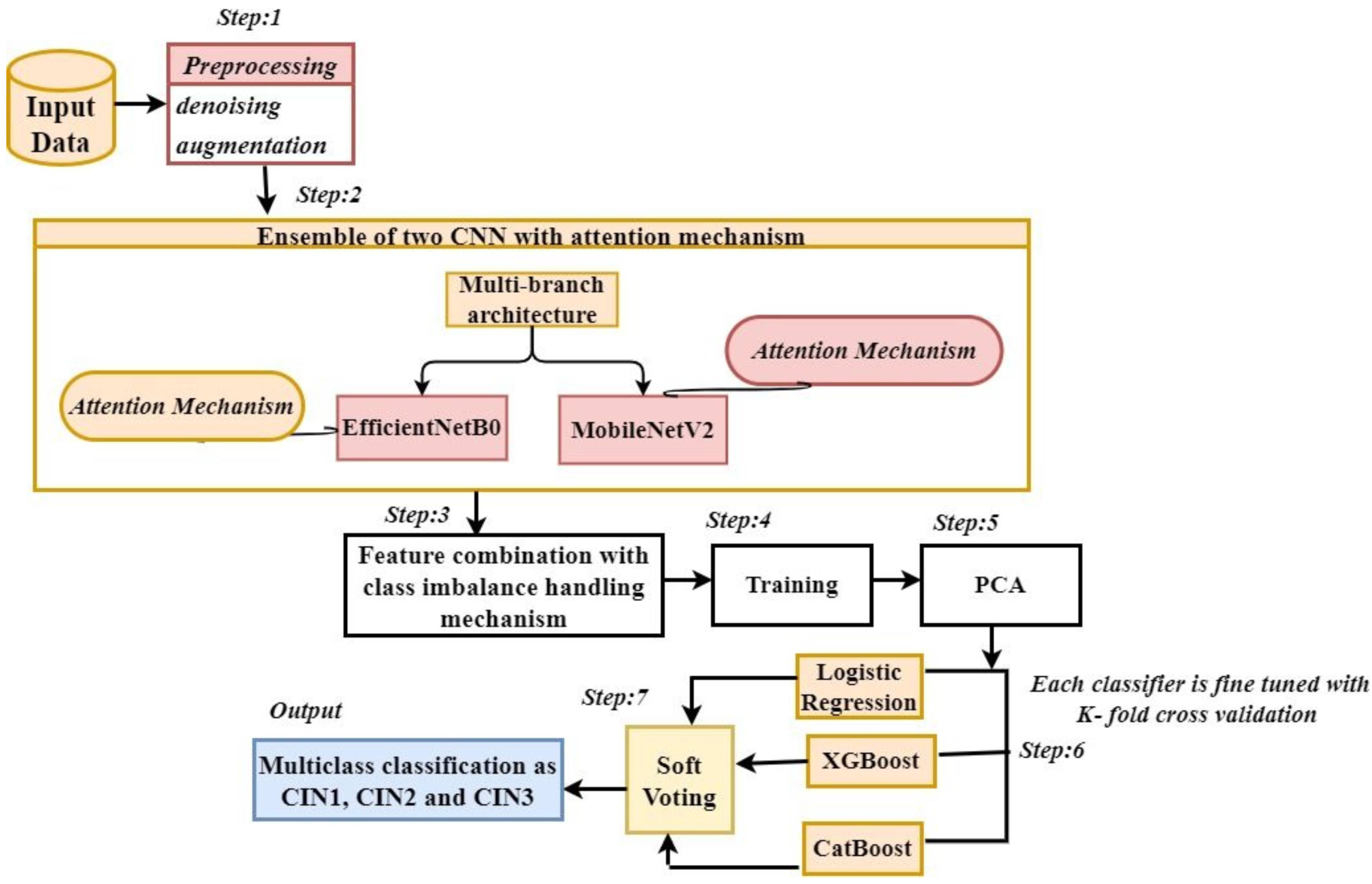
Figure 1. Process flow of the proposed architecture.
Preprints 138279 g001
Figure 2. CIN1, CIN2 and CIN3 distribution of the primary dataset.
Preprints 138279 g002
Figure 3. Sample image of three classes of IARC dataset showing denoising and augmentation.
Preprints 138279 g003
Figure 4. Sample image of three classes of Malhari dataset showing denoising and augmentation.
Preprints 138279 g004
Figure 5. Loss and accuracy trends of the model on primary denoised dataset for the first 50 epochs.
Preprints 138279 g005
Figure 6. PCA visualization plot.
Preprints 138279 g006
Figure 7. AUC curve of the multi-class classification.
Preprints 138279 g007
Figure 8. Confusion matrix plot after ensemble classification on the validation data.
Preprints 138279 g008
Figure 9. Sample images of true and predicted classes with respect to CIN grades on the test data.
Preprints 138279 g009
Figure 10. Loss and accuracy trends of the model on the noisy primary dataset in Lugol’s iodine for the first 50 epochs.
Preprints 138279 g010
Figure 11. Loss and accuracy trends of the model on the noisy primary dataset in Acetic acid for the first 50 epochs.
Preprints 138279 g011
Figure 12. Loss and accuracy trends of the model on the noisy primary dataset in Normal saline for the first 50 epochs.
Preprints 138279 g012
Figure 13. Loss and accuracy trends of the model on the denoised secondary dataset for the first 50 epochs.
Preprints 138279 g013
Table 1. Gaps identified and corrective measures.
Research Gap Description Corrective Measures
1. Flexibility, interpretability , generalizability [25]. The cited model has limited adaptability to different types of features or data; its dense layers make it harder to interpret the influence of individual features and it may overfit due to its reliance on a single deep network. Our model has multi-branch that helps to integrate diverse architectures for richer feature extraction. We have used classifiers like Logistic Regression and feature selection (PCA) allows for clearer insight into how decisions are made. With multiple classifiers, it reduces overfitting, improving generalization across diverse lesion types.
2. Feature extraction and attention mechanism [26]. As per the context of the cited architecture, only ResNet50 is used for feature extraction. While ResNet50 is powerful, it is limited to the feature set learned from a single model. The model does not incorporate an attention mechanism, which is essential in medical imaging to focus on the most critical regions (lesions). Our multi-branch approach leverages both EfficientNetB0 and MobileNetV2, two different architectures trained on large-scale datasets, enabling a richer and more diverse feature representation that better captures different patterns across lesion types. Our model includes attention layers in both branches, allowing it to prioritize key areas in the medical images, improving the detection of subtle lesions.
3. Limited Model Diversity and class imbalance handling [27]. The cited algorithm uses two pre-trained CNN models (DenseNet and ResNet), both of which are powerful for image feature extraction. However, they might still provide similar kinds of features as both are deep convolutional architectures. The algorithm does not mention handling class imbalance, which is a common problem in medical datasets. In our case, the model captures a wider diversity of features, leading to potentially better generalization on medical images with subtle lesion patterns. The algorithm explicitly handles class imbalance by introducing class weights during training, ensuring that all lesion classes (CIN1, CIN2, CIN3) are properly represented and the model doesn’t become biased toward the majority class.
4. Handling lesion cases and dropout [28]. The cited model focuses on general feature extraction and classification without mentioning specific mechanisms for handling class imbalance or lesion-specific processing. The algorithm uses dropout (0.1 probability) to prevent overfitting. While dropout is effective, it operates by randomly disabling neurons, which can potentially drop important feature representations. The attention mechanism in our model makes it inherently better at focusing on the critical regions related to lesions, leading to more accurate predictions for different lesion classes. The attention mechanism provides a more targeted approach to overfitting prevention by focusing only on important features.
5. Absence of Class-Specific Fine-Tuning [29]. The cited algorithm does not mention any fine-tuning or class-specific optimization of the CNN models. It relies on the pre-trained models to extract general features, which may not be tailored to the dataset. Our approach not only incorporates fine-tuning of EfficientNetB0 and MobileNetV2 but also applies attention mechanisms to focus on the most relevant lesion-specific regions. This helps the network adapt better to the cervical cancer dataset and provide more accurate predictions for CIN1, CIN2, and CIN3.[2]
Table 2. A Comprehensive Review of existing techniques for Cervical Cancer Classification
Reference Dataset Method Accuracy Remarks
[30]2024 Colposcopy Deep Learning 94.55% Has used a hybrid deep neural network for segmentation.
[31]2024 All cancer images Deep Learning 99% Has used a hybrid of pretrained CNN, CNN-LSTM, machine learning and deep neural classifiers.
[32]2024 Pap Smear Deep Learning 93% Has used the CerviSegNet-DistillPlus as a powerful, efficient, and accessible tool for early cervical cancer diagnosis.
[33]2023 Pap Smear Deep Learning N/A Employs a lightweight deep learning network known as MLNet, which is based on metaheuristics.
[34]2023 Pap Smear Deep Learning 99.22% Uses deep learning integrated with MixUp, CutOut, and CutMix.
[25]2023 Colposcopy Deep Learning 92% Uses predictive deep learning model.
[35]2022 Colposcopy CNN 87% Used CNN with weighted loss function.
[36]2022 ANN 98.87% Applied artificial jellyfish search to ANN.
[37]2022 Colposcopy CNN,SVM 80% ensemble of U-net and SVM.
[38]2022 Colposcopy and histopathological images AI N/A A review on application of AI on cervical cancer screening.
[39]2021 Colposcopy Deep Learning 92% Uses Deep neural techniques for cervical cancer classification.
[8]2021 Colposcopy Deep Learning 90% Using deep neural network generated attention maps for segmentation.
[40]2021 Colposcopy Residual Learning 90%, 99% Employed residual network using Leaky ReLU and PReLU for classification.
[41]2021 MR-CT Images GAN N/A Uses a conditional generative adversarial network (GAN).
[42]2021 Pap Smear Biosensors N/A Uses biosensors for higher accuracy.
[43]2021 Colposcopy CNN 99% Uses Faster Small-Object Detection Neural Networks.
[44]2021 Pap Smear Deep Convolutional Neural Network 95.628% Constructs a CNN called DeepCELL with multiple kernels of varying sizes.
[45]2020 MRI Data of Cervix Statistical Model - A statistical model called LM is used for outlier detection in lognormal distributions.
[46]2020 Colposcopy CNN 81.95% Employs a graph convolutional network with edge features (E-GCN).
[47]2020 Colposcopy CNN N/A The Squeeze-Excitation Convolutional Neural Network (SE-CNN) is utilized to capture depth features across the entire image, leveraging the SE module for targeted feature recalibration. Furthermore, the Region Proposal Network (RPN) produces proposal boxes to pinpoint regions of interest (ROI).
[48]2020 Colposcopy Pre-trained densenet 96.13% Parameters of all layers are fine-tuned with pre-trained DenseNet convolutional neural networks from two datasets (ImageNet and Kaggle).
[49]2020 Colposcopy CNN 96.13% Uses a recurrent convolutional neural network for classification of cervigrams .
Table 3. Classification Metrics and Formulas.
Metric Formula Description
Recall TP TP + FN The percentage of true positives that are accurately detected
Precision TP TP + FP The percentage of expected positives that turn out to be positive
F1 Score 2 × Precision × Recall Precision + Recall Harmonic mean of precision and recall
Accuracy TP + TN TP + FP + TN + FN The proportion of correct predictions over all instances
Table 4. Original and Augmented values of the primary dataset in different solutions across different CIN grades.
CIN Grades Lugol’s-Iodine Acetic-Acid Normal- Saline
Ori-ginal Aug-mented Ori-ginal Aug-mented Ori-ginal Aug-mented
CIN1 114 898 98 691 83 347
CIN2 119 945 101 700 84 365
CIN3 121 1005 107 705 86 353
Table 5. Secondary dataset distribution across different CIN grades.
CIN1 CIN2 CIN3
Ori-ginal Aug-mented Ori-ginal Aug-mented Ori-ginal Aug-mented
900 1112 930 2009 960 2879
Table 6. Precision, Recall, and F1-Score for each class after training at 100th epoch.
CIN Grades Precision Recall F1-Score
CIN 1 0.9733 0.9723 0.9728
CIN 2 0.9740 0.9750 0.9745
CIN 3 0.9769 0.9798 0.9783
Table 7. Performance Metrics for Logistic Regression, XGBoost, and CatBoost After Hyperparameter Tuning and K=5 fold cross validation
Classifier Fold Accuracy Precision Recall F1 Score
Logistic Regression Fold 1 0.9801 0.9800 0.9789 0.9798
Fold 2 0.9804 0.9801 0.9799 0.9798
Fold 3 0.9810 0.9804 0.9801 0.9800
Fold 4 0.9806 0.9800 0.9798 0.9799
Fold 5 0.9803 0.9801 0.9801 0.9805
XGBoost Fold 1 0.9903 0.9843 0.9844 0.9843
Fold 2 0.9910 0.9903 0.9900 0.9906
Fold 3 0.9904 0.9900 0.9901 0.9902
Fold 4 0.9901 0.9902 0.9900 0.9905
Fold 5 0.9906 0.9900 0.9901 0.9903
CatBoost Fold 1 0.9904 0.9901 0.9900 0.9902
Fold 2 0.9901 0.9904 0.9901 0.9902
Fold 3 0.9908 0.9905 0.9903 0.9903
Fold 4 0.9906 0.9902 0.9901 0.9902
Fold 5 0.9905 0.9903 0.9901 0.9902
Table 8. Performance Metrics for Logistic Regression, XGBoost, CatBoost, and the Ensemble Voting Classifier.
Class-ifier Vali-dation Accuracy CIN1 CIN2 CIN3
Pre-cision Rec-all F1-Score Pre-cision Rec-all F1-Score Pre-cision Rec-all F1-Score
LR 0.9823 0.9815 0.9811 0.9814 0.9902 0.9900 0.9901 0.9904 0.9903 0.9902
XGBoost 0.9905 0.9899 0.9901 0.9901 0.9904 0.9903 0.9904 0.9907 0.9904 0.9904
CatBoost 0.9909 0.9901 0.9900 0.9901 0.9905 0.9903 0.9904 0.9908 0.9906 0.9905
Ensemble 0.9985 0.9995 0.9994 0.9993 0.9996 0.9994 0.9998 0.9998 0.9997 0.9996
Table 9. Performance Metrics of different noisy primary dataset and denoised secondary datasets with respect to CIN Grades.
CIN-Grades Lugol’s Iodine Acetic Acid Normal Saline Malhari
Prec. Recall F1 Prec. Recall F1 Prec. Recall F1 Prec. Recall F1
CIN1 0.97 0.97 0.97 0.96 0.95 0.96 0.95 0.95 0.95 0.98 0.98 0.98
CIN2 0.97 0.97 0.97 0.96 0.97 0.97 0.95 0.94 0.95 0.98 0.98 0.98
CIN3 0.98 0.98 0.97 0.97 0.96 0.97 0.96 0.95 0.96 0.98 0.98 0.98
Table 10. Performance metrics of existing models with respect to CIN grades on primary denoised dataset
Existing Models Val Acc. CIN1 CIN2 CIN3
Prec. Recall F1 Prec. Recall F1 Prec. Recall F1
[25] 0.97 0.95 0.94 0.95 0.96 0.96 0.95 0.97 0.96 0.96
[26] 0.96 0.94 0.92 0.93 0.94 0.93 0.93 0.95 0.94 0.94
[27] 0.95 0.91 0.90 0.91 0.92 0.91 0.91 0.93 0.92 0.92
ResNet50 (baseline) 0.92 0.90 0.89 0.90 0.91 0.90 0.91 0.91 0.90 0.91
DenseNet-121 (baseline) 0.93 0.91 0.90 0.91 0.91 0.91 0.91 0.92 0.91 0.92
EffB0 0.92 0.90 0.89 0.90 0.91 0.89 0.90 0.91 0.90 0.91
MobV2 0.91 0.90 0.88 0.89 0.90 0.89 0.90 0.90 0.90 0.90
EffB0 + MobV2 0.94 0.91 0.90 0.91 0.92 0.91 0.92 0.93 0.91 0.92
EffB0 + MobV2 (with attention) 0.95 0.93 0.92 0.92 0.93 0.92 0.92 0.94 0.93 0.94
Proposed approach 0.99 0.99 0.99 0.99 0.99 0.99 0.99 0.99 0.99 0.99
Disclaimer/Publisher’s Note: The statements, opinions and data contained in all publications are solely those of the individual author(s) and contributor(s) and not of MDPI and/or the editor(s). MDPI and/or the editor(s) disclaim responsibility for any injury to people or property resulting from any ideas, methods, instructions or products referred to in the content.
Copyright: This open access article is published under a Creative Commons CC BY 4.0 license, which permit the free download, distribution, and reuse, provided that the author and preprint are cited in any reuse.
Alerts
Prerpints.org logo

Preprints.org is a free preprint server supported by MDPI in Basel, Switzerland.

Subscribe

© 2025 MDPI (Basel, Switzerland) unless otherwise stated