Development and Comparative Analysis of Machine Learning Models for Hypoxemia Severity Triage in CBRNE Emergency Scenarios Using Physiological and Demographic Data from Medical-Grade Devices

This paper presents the development of machine learning (ML) models to predict hypoxemia severity during emergency triage, especially in Chemical, Biological, Radiological, Nuclear, and Explosive (CBRNE) events, using physiological data from medical-grade sensors. Gradient Boosting Models (XGBoost, LightGBM, CatBoost) and sequential models (LSTM, GRU) were trained on physiological and demographic data from the MIMIC-III and IV datasets. A robust preprocessing pipeline addressed missing data, class imbalances, and incorporated synthetic data flagged with masks. Gradient Boosting Models (GBMs) outperformed sequential models in terms of training speed, interpretability, and reliability, making them well-suited for real-time decision-making. While their performance was comparable to that of sequential models, the GBMs used score features from six physiological variables derived from the enhanced National Early Warning Score (NEWS) 2, which we termed NEWS2+. This approach significantly improved prediction accuracy. While sequential models handled temporal data well, their performance gains didn’t justify the higher computational cost. A 5-minute prediction window was chosen for timely intervention, with minute-level interpolations standardizing the data. Feature importance analysis highlighted the significant role of mask and score features in enhancing both transparency and performance. Temporal dependencies proved to be less critical, as Gradient Boosting Models were able to capture key patterns effectively without relying on them. This study highlights ML's potential to improve triage and reduce alarm fatigue. Future work will integrate data from multiple hospitals to enhance model generalizability across clinical settings.

Keywords:

Subject:

Computer Science and Mathematics - Artificial Intelligence and Machine Learning

Supplementary Material

supplementary.pdf (560.81KB )

1. Introduction

Rapid and accurate patient triage is essential during disaster situations, especially in Chemical, Biological, Radiological, Nuclear, and Explosive (CBRNE) events [1,2,3,4]. These incidents often lead to mass casualties and chaotic environments, overwhelming traditional triage systems. The VIMY Multi-System is a technologically enhanced response platform designed to improve casualty management in these complex scenarios. Initiated at the Grouping in AI acute care for the child (CHU Ste Justine, Montreal, Canada) (https://www.chusj‐sip‐ia.ca/) as part of the VIMY research program, this system leverages artificial intelligence (AI) to manage casualties in disaster settings, including CBRNE events.

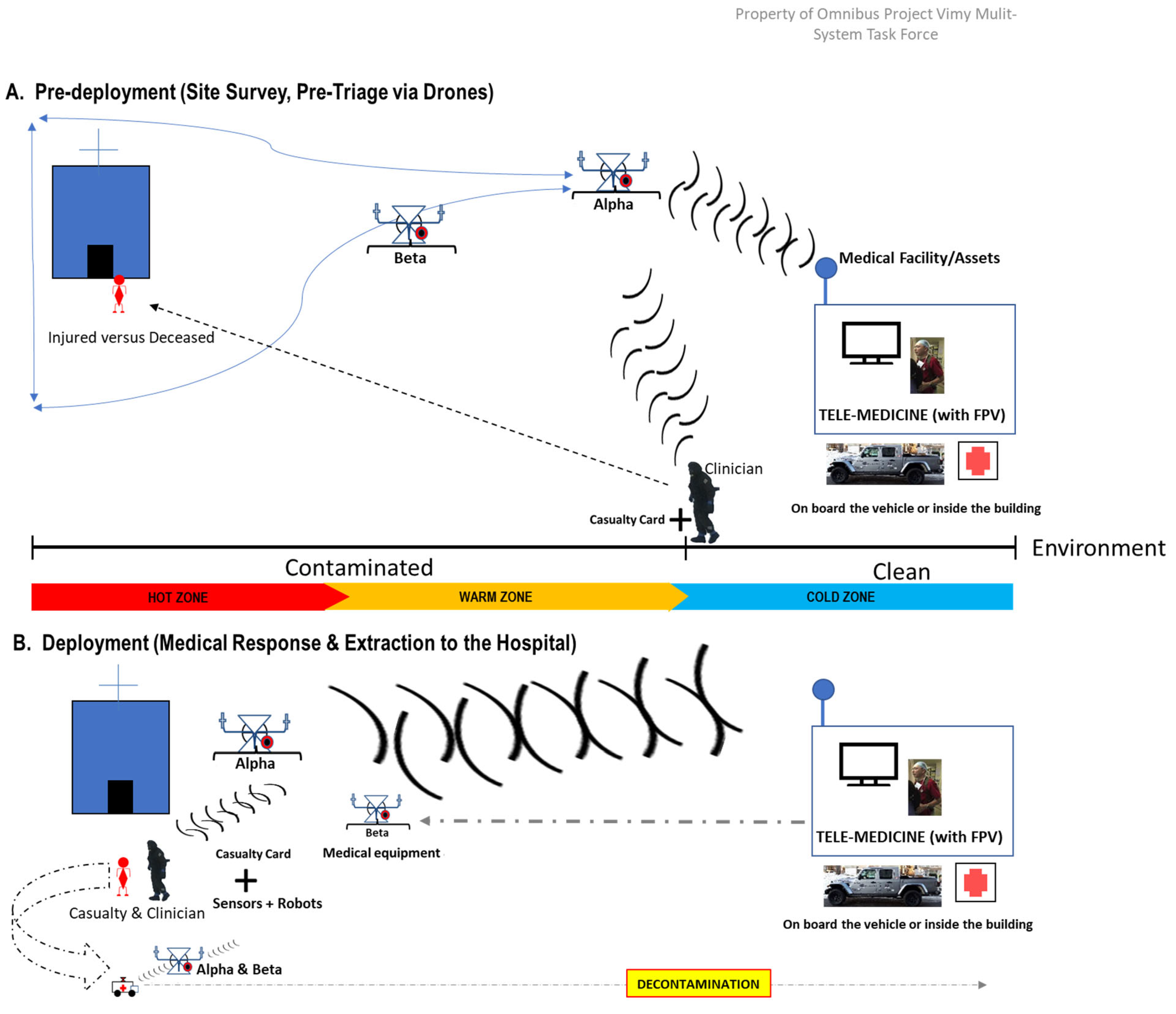
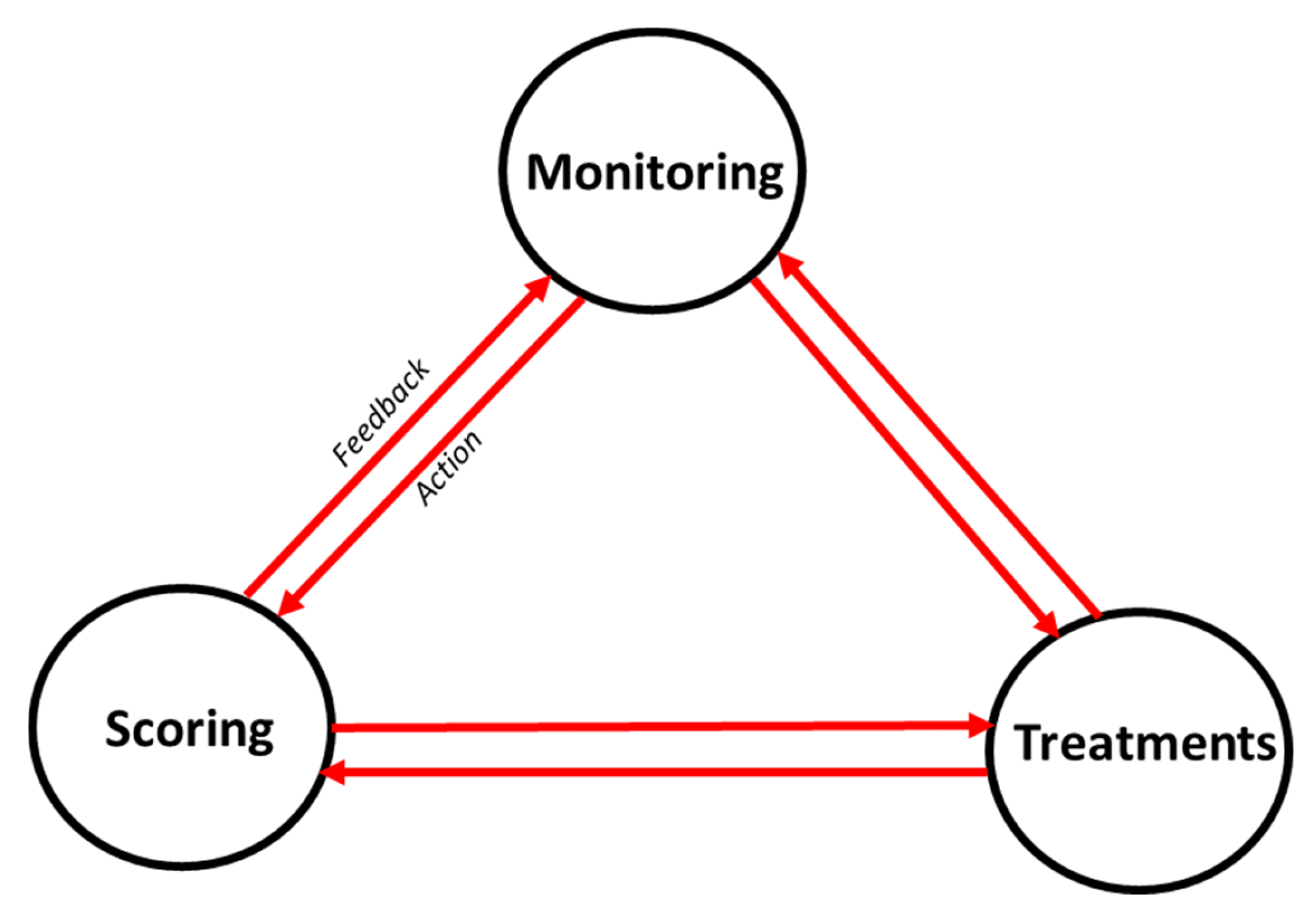
More specifically, the VIMY Multi-System [5,6,7,8] is a field-deployable intensive care unit that integrates AI, sensors, and decision-making algorithms to improve healthcare during disasters (Figure 1). The core framework of the VIMY system incorporates an Electronic Casualty Card System (ECCS), functioning as a dashboard that integrates monitoring, scoring, and treatment data (Figure 2). Its primary aim is to equip frontline personnel with advanced tools to overcome the limitations of current triage and early warning systems (EWS), particularly in CBRNE scenarios, by harnessing machine learning to enhance patient care. This paper specifically focuses on the development of predictive algorithms that are fundamental to the ECCS, thereby contributing directly to the improvement of these critical systems within the VIMY project.

EWS are tools used in healthcare to assess the severity of a patient’s condition by monitoring key physiological parameters, such as heart rate, blood pressure, respiratory rate, temperature, and level of consciousness. EWS helps healthcare providers identify patients at risk of deterioration, enabling timely interventions. By tracking vital signs and assigning scores based on their values, EWS aids in the early detection of patients who may need closer monitoring or medical intervention.

EWS such as NEWS2 [9,10,11,12], PWES [13,14,15,16], the Pediatric Vital Signs Normal Ranges from the Iowa Head and Neck Protocols [17,18], and the Modified Early Warning Score (MEWS) [19,20,21] have been developed to monitor patients' vital signs [11,22,23]. However, existing EWS do not predict the worsening of a patient's condition, which would be crucial for early intervention, especially in pre-clinical scenarios like CBRNE events [11,23,24], where multiple patients are injured simultaneously [24,25]. Thus, EWS are known to have limitations [23,24], even if they are very useful.

Machine learning (ML) offers a promising approach to enhance the predictive capabilities of EWS by analyzing complex physiological data [26,27]. In this study, we present the development of ML-based models using data from medical devices to predict hypoxemia severity, aiming to improve triage efficiency and reduce medical staff fatigue. Our models leverage physiological and demographic data (including age, which influences the medical interpretation of physiological constants), focusing on key vital signs such as respiratory rate, SpO₂ (oxygen saturation) levels, heart rate, both systolic and diastolic blood pressure, and temperature.

Hypoxemia, characterized by low oxygen levels in the blood, is a common and critical condition in disaster settings. Accurate assessment of hypoxemia severity is essential for timely intervention. Current efforts to use ML to predict hypoxic events are happening in various settings and showcasing diverse methodologies. The studies differ considerably in patient populations, outcome definitions, predictive features, and ML algorithms, making it hard to generalize their conclusions. Consequently, comparing and evaluating these studies comprehensively is quite challenging [28]. Indeed, a systematic review compares [28] past efforts to predict hypoxic events in hospital settings using machine learning, focusing on methodologies, predictive performance, and the populations assessed. The authors identified 12 studies that predicted hypoxic events or hypoxia markers across various settings, including operating rooms, ICUs, and general care units. The machine learning models applied were based on both conventional ML and deep learning methods. Most studies defined their prediction endpoints using specific thresholds for blood oxygen measurements. Clinical variables included patient characteristics, vital signs, and laboratory data, with blood oxygen data (such as peripheral oxygen saturation, SpO₂ ) being the most frequently used predictor for hypoxia. However, deep learning and conventional ML methods are not directly comparable, as they were applied to different datasets and performance metrics were inconsistently reported. Additionally, comparability between studies was hindered by the wide variability in approaches, including the differing settings, which introduced various influences on blood oxygen saturation.

Moreover, aheterogeneous medical population is beneficial for developing a broadly applicable predictive model for hypoxia in CBRNE situations, as it increases the likelihood of achieving generalized results.

Additionally, we believe that the assumption that the model may rely on correlations and patterns among features to build its representations—potentially diverging from the established medical gold standards on which Early Warning Scores (EWS) are based—was not sufficiently developed to be considered a fundamental hypothesis.

In medicine, a "gold standard" refers to the most trusted and conventional method for diagnosing diseases, assessing treatment effectiveness, or verifying the accuracy of tests and measurements. This benchmark serves as the reference standard for comparing alternative approaches.

In this study, we used datasets from MIMIC-III and IV [29,30,31], employing Gradient Boosting Models [32,33,34] (XGBoost, LightGBM, CatBoost) and sequential models [35,36,37] (LSTM, GRU) to predict hypoxemia severity scores. These scores, which actually are the labels we aim to predict, were based on the newly designed NEWS2+ system adapted for pre-clinical scenarios, like CBRNE events. This adaptation, defined by medical expert annotations in the VIMY research group, includes hypoxemia severity for three population groups (adults with COPD, adults without COPD, and pediatric patients without COPD) and a modified EWS for two population groups (adult and pediatric patients). Our comprehensive preprocessing pipeline addressed missing data and class imbalances, ensuring robust and reliable model training.

This paper is structured as follows: Section 2 details the materials and methods, including data preprocessing and model development. Section 3 presents the results of our experiments. In Section 4, we discuss the implications of our findings. Finally, Section 5 concludes the study and outlines future research directions.

2. Materials and Methods

2.1. Data Sources

We used the MIMIC-III and MIMIC-IV databases [29,30,31], which are extensive, de-identified health records of ICU patients. MIMIC-IV is an excellent choice for beginners or those seeking to leverage well-established concepts, as it offers a robust and widely used dataset. However, while the HiRID database provides data at 2-minute intervals, MIMIC remains the most comprehensive dataset, offering greater breadth and depth for a variety of clinical research applications.

Given that, to our knowledge, no public physiological dataset has been collected specifically in a CBRNE context, we used ICU data for this proof of concept. Critical care patients frequently exhibit severe distress patterns akin to those expected in CBRNE scenarios, making this data a suitable proxy.

Furthermore, we have a very heterogeneous population, which can actually be beneficial, as our goal is to predict hypoxia in CBRNE situations in a non-specific manner. Indeed, rather than targeting a single scenario, we aim to develop a broadly applicable predictive model. Thus, a diverse population increases the likelihood of achieving broadly applicable results, enhancing the overall scope of our predictive model.

Finally, the MIMIC-III dataset includes around 58,000 hospital admissions for over 40,000 unique patients, while MIMIC-IV expands this to over 380,000 admissions for more than 210,000 patients from 2008 to 2019. Both databases offer detailed information, including continuous vital sign monitoring (recorded regularly or very frequently), laboratory results, and demographic details, making them highly applicable to our hypoxemia prediction study.

2.2. Inclusion Criteria and Data Representativeness

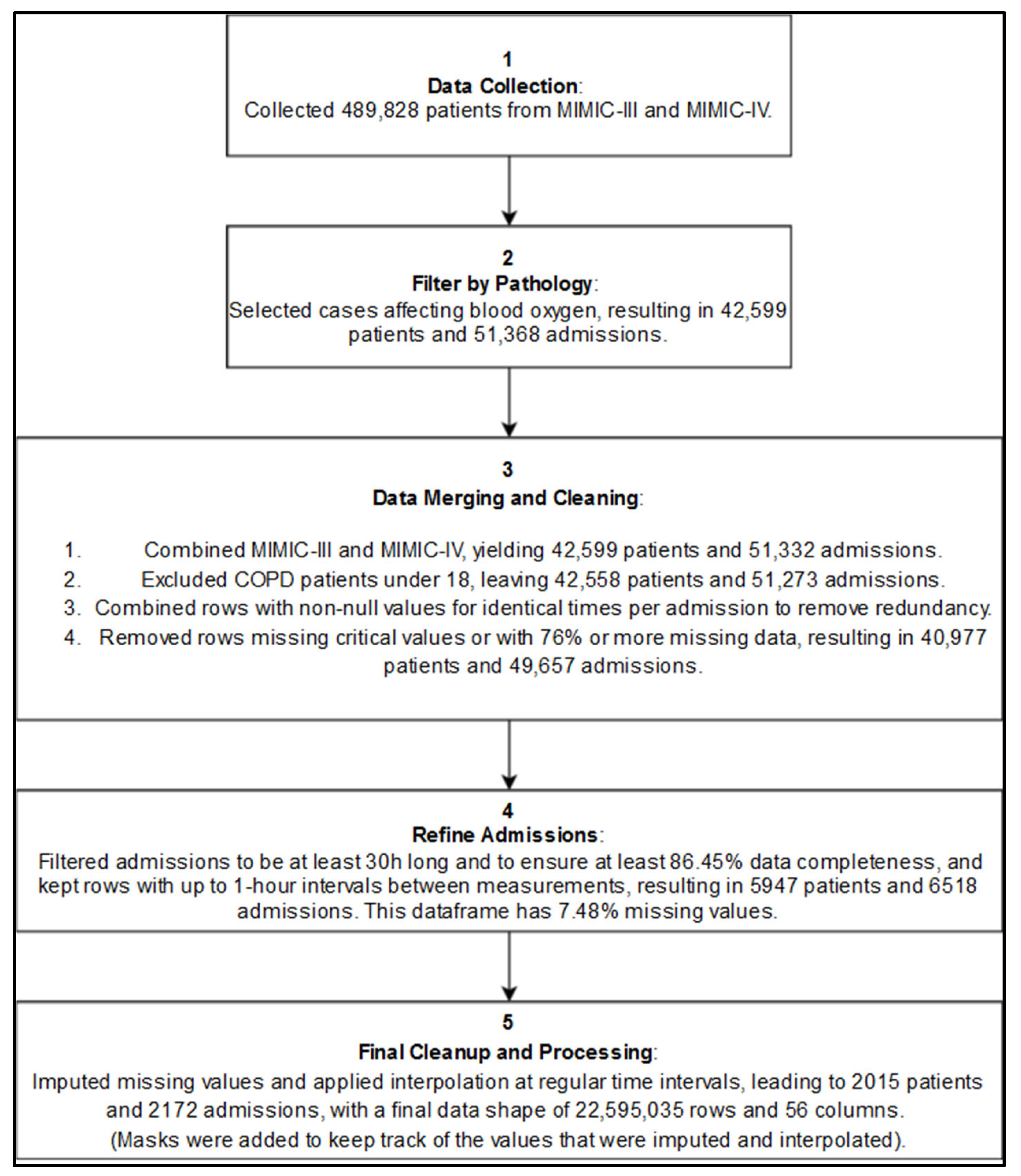
Patients were included if they had recorded episodes of hypoxemia or were diagnosed with conditions very often associated with potential low blood oxygenation levels, which made them more likely to experience hypoxemic episodes (see appendix, A6). A total of 51,368 admissions from 42,599 unique patients were selected based on the International Classification of Diseases (ICD) codes related to hypoxemia and respiratory distress. Figure 3 illustrates the simplified inclusion process.

2.3. Data Preprocessing

2.3.1. Labeling and Feature Engineering

The VIMY project research team has initiated a new research wing focused on triage and early-warning systems to support the development of the NEWS2+ early warning system. NEWS2+ is an extension of the original NEWS2, being revisited in light of recent advancements in the scientific literature, and relevant to pre-clinical contexts. Specifically, the medical experts on the team have focused on adapting the original NEWS2 parameters for application in acute pre-hospital environments. We have developed an alternative method to “inform” the model about what constitutes a trigger value for the physiological variables in question, incorporating an alarm mechanism. Additionally, temporal information is provided for each physiological variable of interest, detailing how long each alarm persisted. Medical experts within the VIMY team have contributed significantly to this initiative, and the adapted chart will be extended for use in disaster scenarios, including CBRNE events.

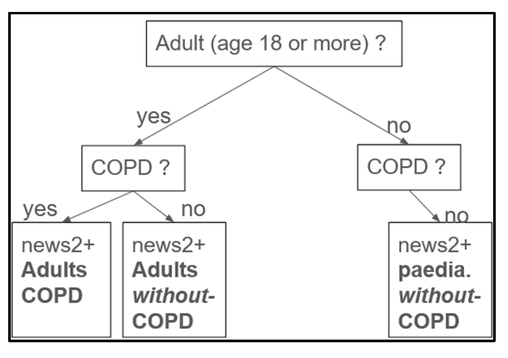
Use of SpO₂ for categorization. To categorize hypoxemia severity, we introduced a severity labeling column based on SpO₂ values, classifying patients as severe, moderate, mild, or normal. SpO₂ was chosen as the central parameter due to its prevalence and accessibility through oximeters in pre-hospital and acute care scenarios. The system assigns scores ranging from 0 (normal) to 3 (severe) based on SpO₂ levels, with adjustments for patient age and the presence or absence (Figure 4) of chronic obstructive pulmonary disease (COPD).

In certain situations, gold-standard thresholds need to be adapted based on advancements in the literature. For instance, Dempsey et al. [38] described hypoxemia levels in healthy individuals as follows: mild (93-95%), moderate (88-93%), and severe (<88%). Bourassa et al [8] proposed hypoxemia thresholds of <90% for the general population and <88% for COPD patients in room air conditions [8]. They also set hypoxemia thresholds for supplemental oxygen therapy at >92% for the general population and >94% for those with COPD.

Additionally, Johannigman et al. [39] reported notable changes in SpO₂ during aeromedical evacuations, where 90% of military personnel experienced at least one desaturation event with SpO₂ <90%, and over half dropped below 85%

From the medical conditions manually selected in the MIMIC database, COPD cases were identified based on the presence of the following conditions: Chronic Obstructive Respiratory Disease, COPD arising in the perinatal period, Chronic obstructive asthma with status asthmaticus, and Other chronic bronchitis, which could have an impact on the SpO2 level in basal state.

The Table 1 displays the adapted values for different hypoxemia levels in adults with and without COPD, as well as in the pediatric population without COPD (pediatric population with COPD is not considered in this study). By providing tailored SpO₂ thresholds for varying patient needs, the NEWS2+ scoring matrices support comprehensive hypoxemia risk assessment and facilitate targeted clinical responses across diverse patient populations.

The NEWS2+ scoring matrices provide a structured approach to determining hypoxemia severity scores across distinct patient groups, specifically tailored for adults without COPD, adults with COPD, and pediatric populations. These scores serve as the labels we aim to predict within our study and are grounded in established research sources [4,8,9,10,11,12,13,17,20,40], with further adaptation by physicians to suit a pre-clinical setting. The matrices provide a patient-type-specific framework for interpreting SpO₂ thresholds, which are essential for assessing respiratory health. SpO₂, or oxygen saturation, represents the percentage of oxygenated hemoglobin in the blood, a vital indicator of respiratory function. Each matrix within NEWS2+ is optimized for different oxygenation needs: adults without COPD have specific SpO₂ targets aligned with general adult respiratory requirements; adults with COPD have adjusted targets reflecting the lower oxygenation needs typical for COPD patients; and pediatric populations have age-specific thresholds to accommodate children’s unique respiratory profiles. Each matrix categorizes SpO₂ levels into severity classifications to guide clinical assessment and intervention. Severe hypoxemia indicates critically low SpO₂, requiring immediate medical intervention. Moderate hypoxemia reflects moderate oxygen depletion, necessitating close monitoring and potential intervention. Mild hypoxemia signifies slightly low oxygen levels, usually manageable without intensive treatment. Normal levels denote stable SpO₂ and healthy respiratory function, not requiring intervention.

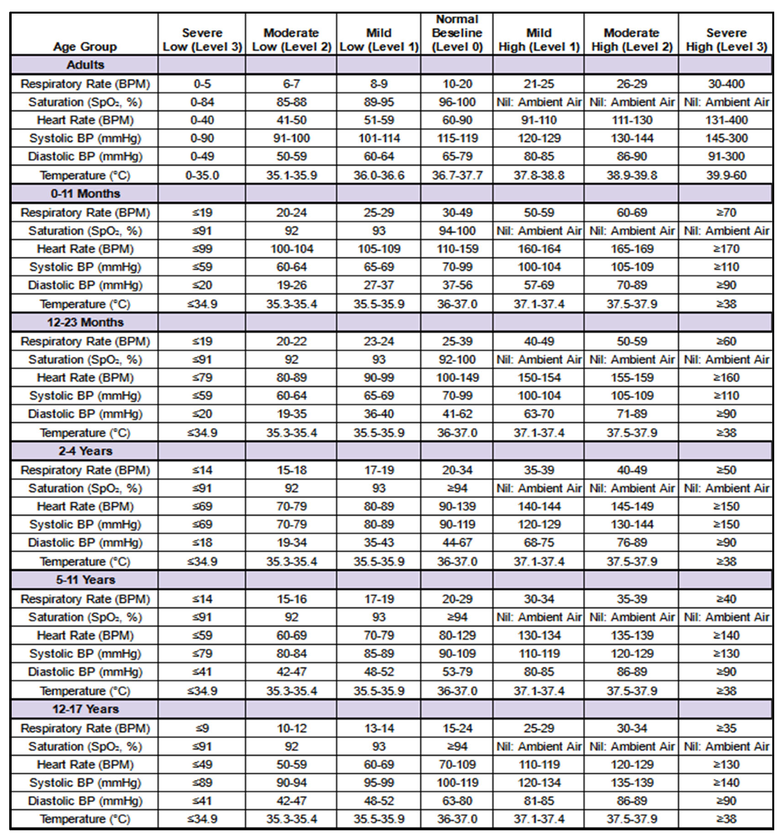
Feature Engineering The Table 2 introduces NEWS2+, an expanded version of the National Early Warning Score 2 (NEWS2), designed to provide a comprehensive assessment of patient status. Developed with guidance of the VIMY team’s medical experts, NEWS2+ evaluates vital signs using specific thresholds and severity levels derived from established Gold Standards. The matrices presented outline the NEWS2+ scoring system applied to six primary physiological variables—respiratory rate, oxygen saturation (SpO₂), heart rate, systolic blood pressure, diastolic blood pressure, and temperature. These scores function as indicators of abnormal vital signs, supporting enhanced data interpretation and predictive modeling.

Each physiological variable is assigned a score reflecting its deviation from age-adjusted reference values, offering critical insights for hypoxemia prediction. These NEWS2+-derived feature scores, occasionally referred to as “TAG” for each physiological variable, may be used interchangeably in this work.

The Table 2 below presents the NEWS2+ matrices used to generate these score features (TAGs), demonstrating the process of assigning individual scores to each physiological variable.

Populations. The NEWS2+ scoring system is applied to derive feature scores (TAGs) for six primary physiological variables across both adult and pediatric populations. For adults, these feature scores capture key indicators of physiological health, while the pediatric version of NEWS2+ is tailored to accommodate developmental differences across specific age groups. The pediatric matrix is divided into five distinct age groups to ensure age-appropriate scoring: infants under 1 year (0–11 months), toddlers under 2 years (12–23 months), children aged 2 to 4 years, those aged 5 to 11 years, and adolescents aged 12 to 17 years. These age groups are presented sequentially, from top to bottom, in the order listed. This structured approach ensures that the scoring accurately reflects physiological expectations and variations across developmental stages, supporting precise assessment and appropriate clinical responses.

2.3.2. Handling Missing Data and Masks

A comprehensive pipeline addressed missing data through imputation and interpolation methods. Missing data accounted for 7.48% of the dataset. We employed a multivariate imputation strategy: Multiple Imputation by Chained Equations (MICE) [41,42,43] using Histogram-based Gradient Boosting.

Synthetic data entries were flagged using masks to ensure transparency, in line with recommendations from previous research [42,43,44,45], which are critical for trust in AI-driven decision-making [46]. This approach helps inform the model about which values were imputed, improving interpretability. Specifically, each feature column had an associated mask column, where a value of 0 indicated no synthetic data and a value of 1 indicated the presence of synthetic data in that row.

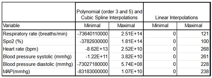
To address irregular time intervals between measurements, we used interpolation to generate regular time series data. Minute-level interpolations were performed using linear interpolation, chosen after comparing it with polynomial and cubic spline methods. Linear interpolation produced the most reliable results for vital signs data, minimizing the risk of implausible physiological values (Table 3).

We observed a typical distribution of maximum values resulting from polynomial interpolations of orders 3 and 5, noting the occurrence of negative values—anomalous in this context—as well as an implausible order of magnitude. Similar issues were found with cubic spline interpolations. In contrast, linear interpolation displayed a typical distribution in which all values remained positive, with an order of magnitude that appropriately reflected the extreme physiological conditions possible in ICU settings. Therefore, we ultimately selected linear interpolation for our analyses.

We added a mask for the charttimes —the timestamps (at the minute) corresponding to when each set of measurements was recorded— indicating which rows were interpolated, to inform the models about synthetic data (same logic as for the imputed values before). This approach aligns with the intuition that linear interpolation can effectively represent gradual changes in a patient's condition between successive measurements.

2.3.3. Sliding Window

To determine an appropriate time window for prediction, we analyzed the average duration of each hypoxemia severity level after interpolation. The mean and median durations for severity scores 0 to 3 were calculated, with severity score 3 having a mean duration of 114.8 minutes and a median of 60.0 minutes. Drawing from these observations, practical considerations, discussions with our team’s medical expert, and findings from previous studies [28,47,48], we established a 5-minute prediction window as the standard for our models. This timeframe is long enough to allow doctors sufficient time to intervene, while remaining short enough to capture near-term risks that require immediate attention. Additionally, it minimizes the risk of inaccurately predicting events that are too far in the future. This balance ensures timely and actionable medical interventions.

2.3.4. Data Cleaning and Transformation

Duplicated Rows and Admissions Removal: To address potential redundant rows introduced during preprocessing, we merged rows with non-null values recorded at the same charttime (i.e., the same timestamp) within each admission. For eventual duplicate admissions across the combined MIMIC III and IV datasets (which may have different admission IDs), only the most recent occurrence of each redundant row (considering all physiological and demographic features) was retained, while earlier rows were removed to maintain data consistency. This approach ensures that, for each potentially redundant admission, only a single, complete version remains in the final dataset, effectively eliminating duplicate admissions on a row-by-row basis.

Outlier Handling: Implausible physiological measurements were replaced with NaN and subsequently imputed to address potential human errors in the electronic health records. Specifically, for six key vital signs variables, we excluded values outside defined ranges: respiratory rate, heart rate, and both systolic and diastolic blood pressure above 300 or below 0; SpO₂ above 100 or below 0; and temperature readings above 60 or below 0. To ensure consistency, this step was applied both before and after imputation and interpolation.

Data Rounding: Physiological values were rounded in order to standardize precision, which supports model generalization and may reduce the likelihood of overfitting, especially as future work integrates data from additional hospitals.

Missing values: Imputation by Chained Equations (MICE) using Histogram-based Gradient Boosting were done to complete the 7.48% missing values from our preprocessed dataframe

Time Alignment: Interpolated data at minute-level intervals to standardize time steps across admissions (synthetic data).

2.3.5. Data Splitting

To ensure robust comparisons and avoid data leakage, patient data was split into training, validation, and testing sets, ensuring no patient appeared in more than one set (patient wise not admission wise). Specifically, 75% of patients were allocated to the training set (2,015 patients), while the validation and test sets each comprised 12.5% of the patients (212 patients each).

2.4. Exploratory Data Analysis (EDA)

We conducted EDA to understand data distributions and correlations:

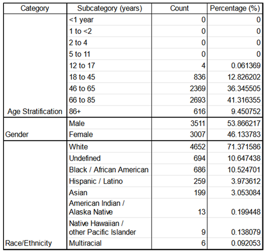
Demographics: Table 4 illustrates the patients’ age, gender, race, and ethnicity distributions.

Concerning the demographics, for the races and ethnicities, we referred to the United States Census Bureau[49].

The age stratifications shown below were a constitution work from various sources [50,51] and were used to do the NEWS2+ derived features scores (TAGS) for the six key physiological parameters.

The top panel illustrates age stratification across admissions, revealing no pediatric patients, four teenage admissions, and predominantly adult admissions. Most adults are between the ages of 45-65 or 66-84, with a slightly higher proportion of elderly individuals (66+). Age groups are categorized as infant (0-17 years), adult (18-65 years), and elderly (65+ years). The middle panel shows gender distribution, with a moderate overrepresentation of males compared to females. The bottom panel presents the distribution of race and ethnicity, highlighting an overrepresentation of white individuals. Here, "Hispanic/Latino" is categorized as an ethnicity, while other categories are classified by race.

Label Distribution: We observed an unbalanced dataset, where higher severity scores occur less frequently (Table 5). The labels, defined as 0 (normal), 1 (mild), 2 (moderate), and 3 (severe), each represent a specific hypoxemia severity score. They are based on the NEWS2+ scoring system in respect to the Spo2, age and type of disease (see feature engineering, part 2.3.1).

Left columns : before; Right columns : after. The count numbers increase due to the minute-by-minute interpolations adding more rows. However, the label distribution, in terms of percentage, remains very similar and retains its characteristics, making it suitable for later training. The imputations (done before interpolations) and the interpolations did not change the label distribution.

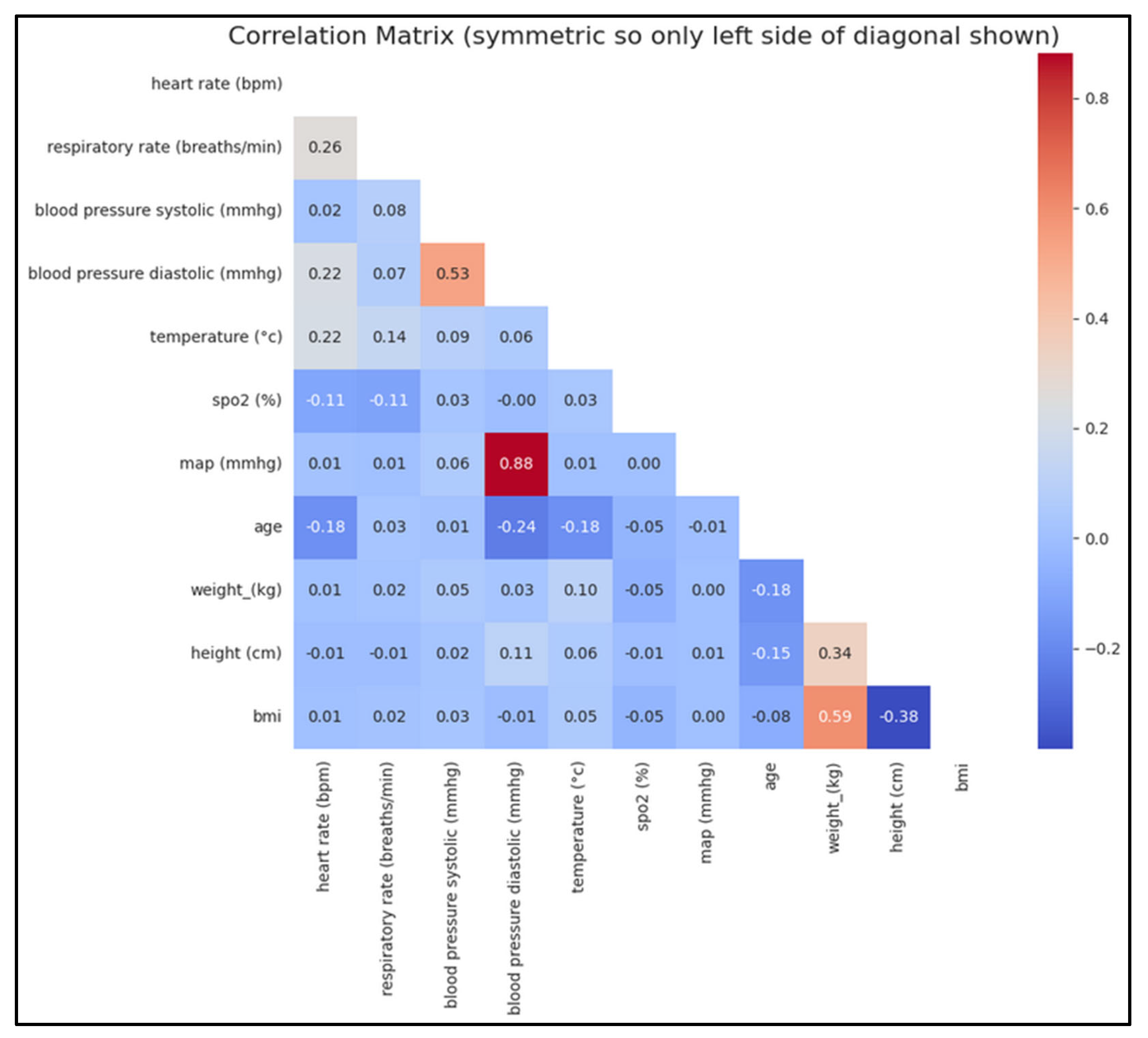
Correlation Analysis: We generated correlation matrices to assess relationships between physiological variables (Figure 5).

There is a strong positive correlation between mean arterial pressure (MAP) and diastolic blood pressure (BP), which is expected since MAP is derived from both diastolic and systolic BP (mathematical relation). Similarly, a strong positive correlation between systolic and diastolic BP aligns with physiological norms. As anticipated, weight and BMI are also strongly correlated, given that BMI is calculated from weight. Conversely, a negative correlation between BMI and height is observed, as BMI decreases with increasing height. Additionally, within a certain age range, a negative correlation between age and diastolic BP can be expected. These correlations underscore the physiological relationships between these variables. Both BMI and MAP are physiologically significant and may provide valuable insights for predicting the risk or severity of hypoxemia.

2.5. Principal Component Analysis (PCA)

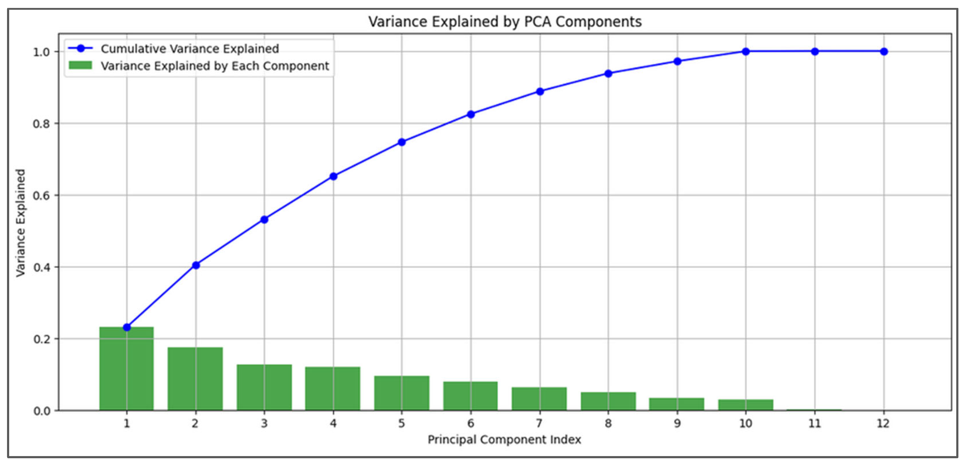
PCA was performed after imputation and interpolation to assess the variance explained by each principal component and feature contributions. Due to PCA’s sensitivity to data scaling, we applied standardization beforehand. The cumulative variance from the first few components indicated that a reduced feature set could capture most data variability (Figure 6). We focused on physiological variables and easily obtainable features (e.g., gender, height, weight) relevant to CBRNE disaster scenarios, excluding other features for this analysis. While PCA is a linear technique and medical data can show non-linear properties, the results provide useful insights into our physiological features, though they should be interpreted cautiously.

2.6. Model Development

2.6.1. Model Selection and Rationale

We selected five models for comparison: Gradient Boosting Models (XGBoost [34], LightGBM [32], CatBoost [33]) and sequential models (LSTM [37] and GRU [36]). The choice was motivated by recent studies demonstrating the effectiveness of both GBMs and sequential models in handling medical time series data [52,53,54,55,56].

The Gradient Boosting Models (GBMs) are effective for tabular data and can handle complex, non-linear relationships. The Sequential Models are designed to capture temporal dependencies in sequential data.

2.6.2. Gradient Boosting Models (GBMs)

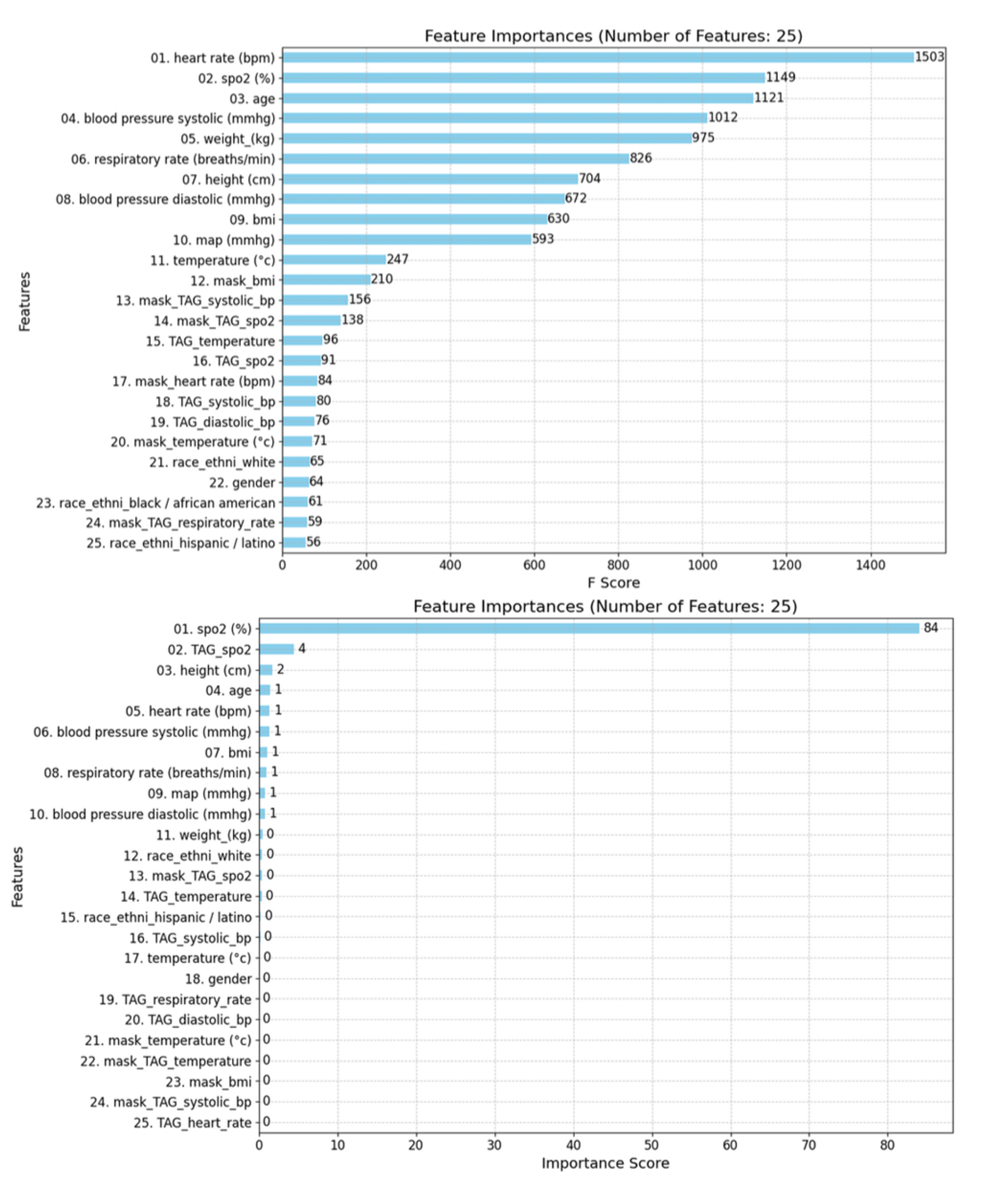
We implemented XGBoost, LightGBM, and CatBoost classifiers. These models are ensemble methods that build upon decision trees, focusing on correcting errors of previous models in the sequence. They offer advantages such as handling missing values and providing feature importance (Figure 10). Note that the shift lag process for the labels was applied for both GBMs and sequential models (see the Figure 8 for the shift lag and 2.6.4 part for further explanations).

The GBMs each offer unique features suited to specific modeling challenges. For instance, XGBoost applies early stopping and class weights to address class imbalance, CatBoost handles categorical variables effectively and reduces prediction shifts, and LightGBM is optimized for speed with Gradient-based One-Side Sampling.

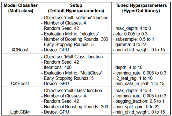
The hyperparameters were optimized using the HyperOpt library and subsequently added to the existing default parameters. This table presents the search ranges of the hyperparameters used to identify the optimal combination for each model (see Table 9 for the best results).

2.6.3. Sequential Models

We implemented Masked LSTM and Masked GRU models to process sequential data, addressing variable sequence lengths through padding and the masking process.

More specifically, among the 2,169 unique admissions in the three datasets, sequence lengths—representing the duration of each admission—ranged from 952 to 254,643 rows, with a median of 5,941 rows and an average of 10,417 rows (each row corresponding to one minute per admission). Thus, a significant difference in terms of the length.

To ensure computational efficiency of the sequential models, we standardized the sequence length to 1,024 rows—about 18 hours per admission. Longer sequences were split into 1,024-row segments, while shorter ones were padded with a constant value of 1000, which didn’t overlap with any actual feature values. This preprocessing generated 23,099 admissions suitable for sequential models.

The Masked LSTM and GRU models were designed to ignore padded values (set to 1000) using an internal mask within the Dataloader. This mask excludes padded values in sequential input data, ensuring they do not influence model training. Notably, this type of "masking" differs from the masks used to identify imputed or interpolated (synthetic) data (see Section 2.3.2).

Variable-length sequences are effectively managed through masking and sequence packing. Sequence lengths are calculated from the mask, and sequences are sorted by length. Using PyTorch's pack_padded_sequence, sequences are packed so that LSTM/GRU layers only process valid time steps, omitting padding from computations. After processing, sequences are unpacked and returned to their original order, enabling efficient batch processing of variable-length sequences and ensuring that padding does not interfere with the model’s learning.

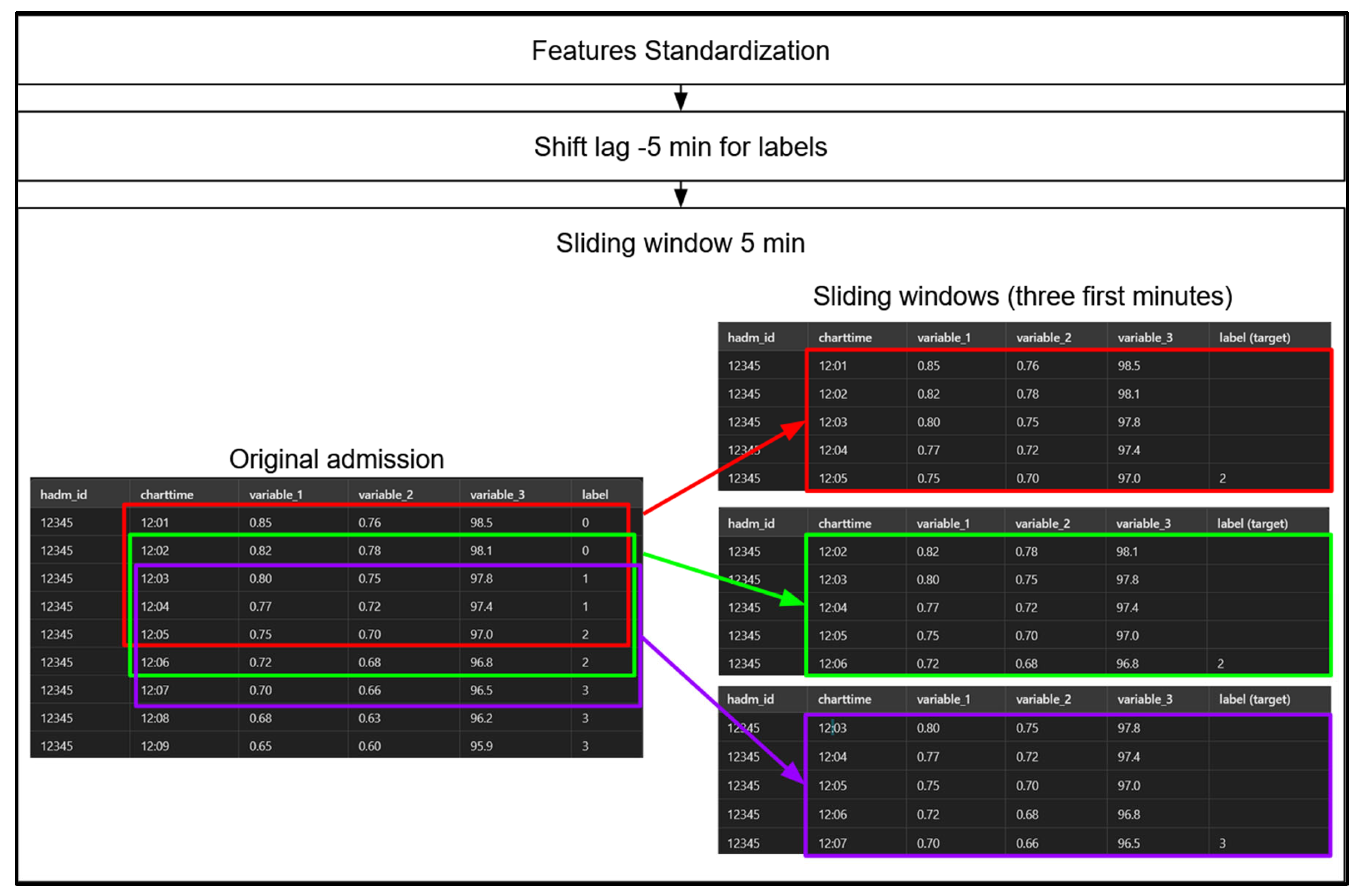
See Figure 7 for an overview of the preprocessing steps for the sequential models.

Step 1: involves standardizing the data using Scikit-Learn’s StandardScaler, but only for our sequential models. Models based on decision trees, such as gradient-boosted machines (GBMs), operate based on threshold values, so standardization is unnecessary for them. Step 2 : we apply a -5-minute shift to the label values, pairing each row with the label occurring 5 minutes later. This adjustment allows each row, representing a set of physiological measurements at a specific minute of a patient’s admission, to serve as the input for predicting the hypoxemia severity score 5 minutes in advance. Notably, this label-shifting process is performed for both sequential models and GBMs. Step 3 : we create 5-minute sliding windows for our sequential models only, as GBMs do not leverage temporal sequences. Each sequential model therefore considers a 5-minute sequence of admission data at a time to predict the hypoxemia severity score label 5 minutes ahead. We then “jump” forward by one row (or one minute), creating a 4-minute overlap between consecutive windows, and repeat this process until we reach the end of the data for each patient admission.

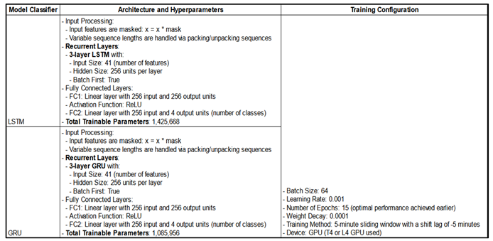
Additional characteristics of the models are presented in Table 7 below.

The “masked” layers use an internal Dataloader mask to exclude padded values in sequential input data, ensuring they are not considered during training. Variable-length sequences are handled through packing and unpacking: a mask ignores padding, and pack_padded_sequence enables LSTM/GRU layers to process only valid steps. After processing, sequences are unpacked to their original order, preventing padding from affecting learning. Due to long training times, hyperparameters were not extensively optimized; instead, a sufficiently complex architecture was implemented, aimed at fitting the training data well enough to demonstrate proof of concept.

2.6.4. Experiments' Setup

To prevent data leakage, we ensured that each patient's data appeared in only one of the training, validation, or testing sets. Admissions were split accordingly.

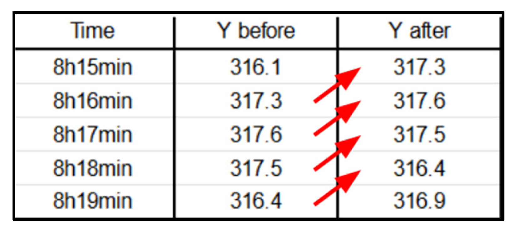
Shift-Lag Method: Applied to predict hypoxemia severity scores 5 minutes in advance, providing a practical window for medical intervention (Figure 8). Indeed, in order to predict hypoxemia severity scores in advance, we apply a -5-minute shift to the label values, aligning each row with the label observed 5 minutes later. This adjustment allows each row, containing physiological measurements recorded at a specific minute of a patient’s admission, to be used as input for predicting the hypoxemia severity score 5 minutes ahead. Importantly, this label-shifting technique is consistently implemented for both sequential models and gradient-boosting machines (GBMs).

Class Imbalance Handling: Computed class weights inversely proportional to class frequencies.

Hyperparameter Tuning of the GBMs: We used the HyperOpt library, a popular tool for hyperparameter optimization, with two objective functions—AUC-based and log loss-based. HyperOpt employs the Tree-structured Parzen Estimator (TPE), a Bayesian optimization technique that iteratively updates a probabilistic model based on prior evaluations and performance metrics. Unlike traditional methods that treat these evaluations as independent, TPE refines its model progressively to capture the relationship between hyperparameters and performance, enhancing optimization efficiency.

AUC-Based: This function focuses on maximizing the AUC score by minimizing 1 - AUC, which is especially beneficial when dealing with class imbalance.

Log Loss: This function minimizes log loss (cross-entropy loss), assessing how closely the predicted probabilities match the actual labels, and penalizing incorrect or overly confident predictions.

2.6.5. Feature Importance Analysis

For the GBMs, the feature importance was assessed to understand the contribution of each feature to the models' predictions. Both TAGs derived from NEWS2+ (Table 2) and mask features indicating synthetic data were included (no masks for the CatBoost models). This analysis helps in interpreting GBMs decisions and ensuring that critical features are appropriately weighted.

3. Results

3.1. Dataset Characteristics

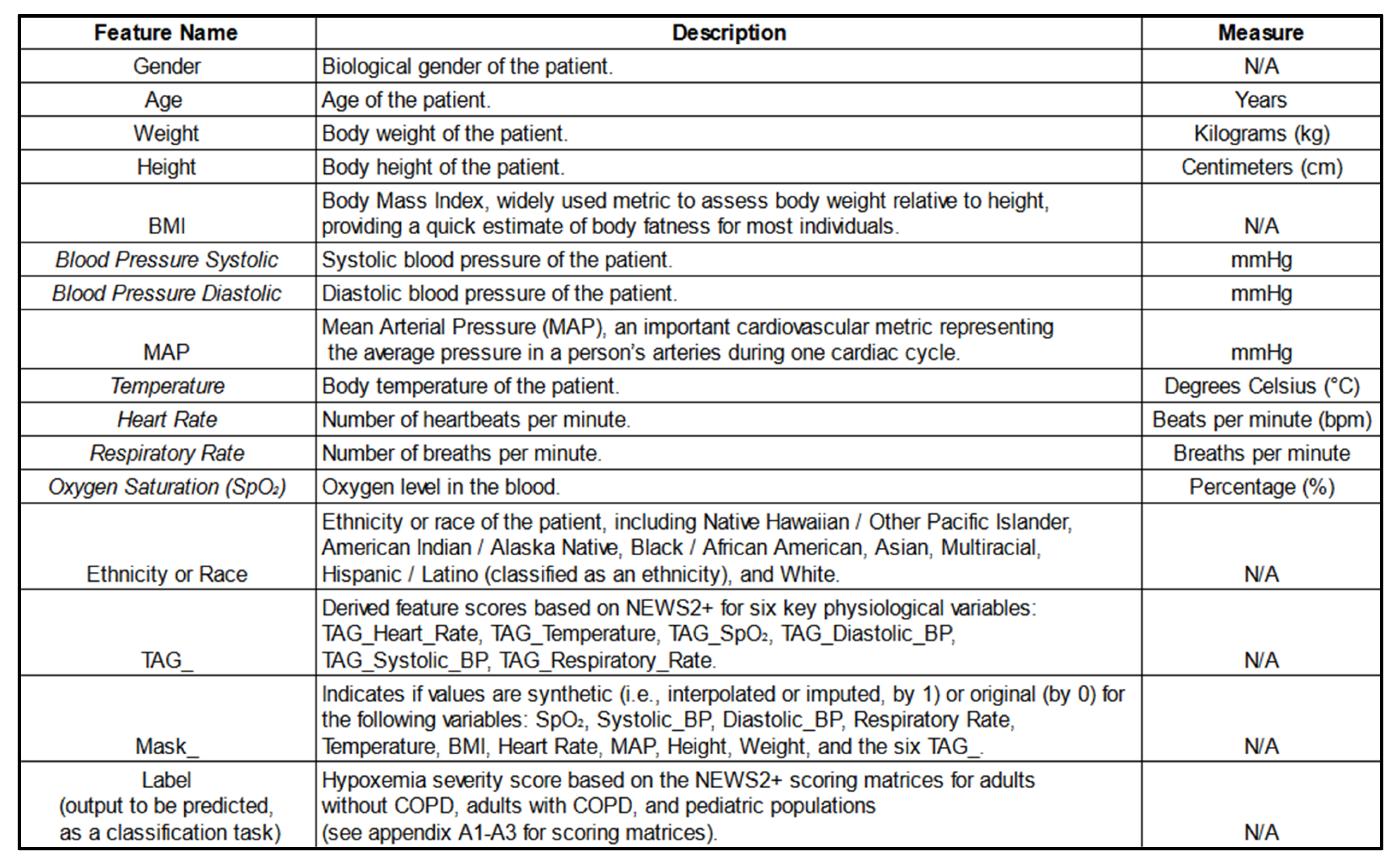
After preprocessing, the dataset consisted of 22,595,035 rows and over 40 feature columns, encompassing both original and engineered features. These features included physiological variables, NEWS+ derived scores (TAGs), demographic data, and mask features (the list of features is available in Table 8 below).

Each admission was interpolated to minute-level intervals, resulting in a substantial increase in data volume. The length of admissions varied, ranging from approximately 16 hours to 177 days for the GBMs. However, for the sequential models, all admission durations were standardized to approximately 16 hours by padding shorter admissions and truncating longer ones.

3.2. Imputation and Interpolation Outcomes

Different imputation strategies were compared. The Histogram-based Gradient-boosting imputation yielded satisfactory results and was selected for further analysis. Imputations reduced the percentage of missing values to zero, enabling subsequent interpolation at the minute level.

Linear interpolation was chosen over polynomial and cubic spline interpolations due to its ability to produce plausible physiological values (Table 3). Polynomial and cubic spline interpolations resulted in implausible negative values and incorrect magnitudes.

3.3. Exploratory Data Analysis Findings

The dataset exhibited an inherent imbalance, with the distribution of severity scores remaining consistent both before and after interpolation. More severe scores were less frequent, reflecting this imbalance. In terms of label durations, severity score 2 had the shortest median duration of 29 minutes, while severity score 0 had the longest median duration, lasting 178 minutes.

3.4. Model Performance

3.4.1. Gradient Boosting Models' Results and Discussion

The GBMs demonstrated strong performance in predicting hypoxemia severity. Hyperparameter tuning yielded only slight improvements over baseline models.

Training and Convergence:

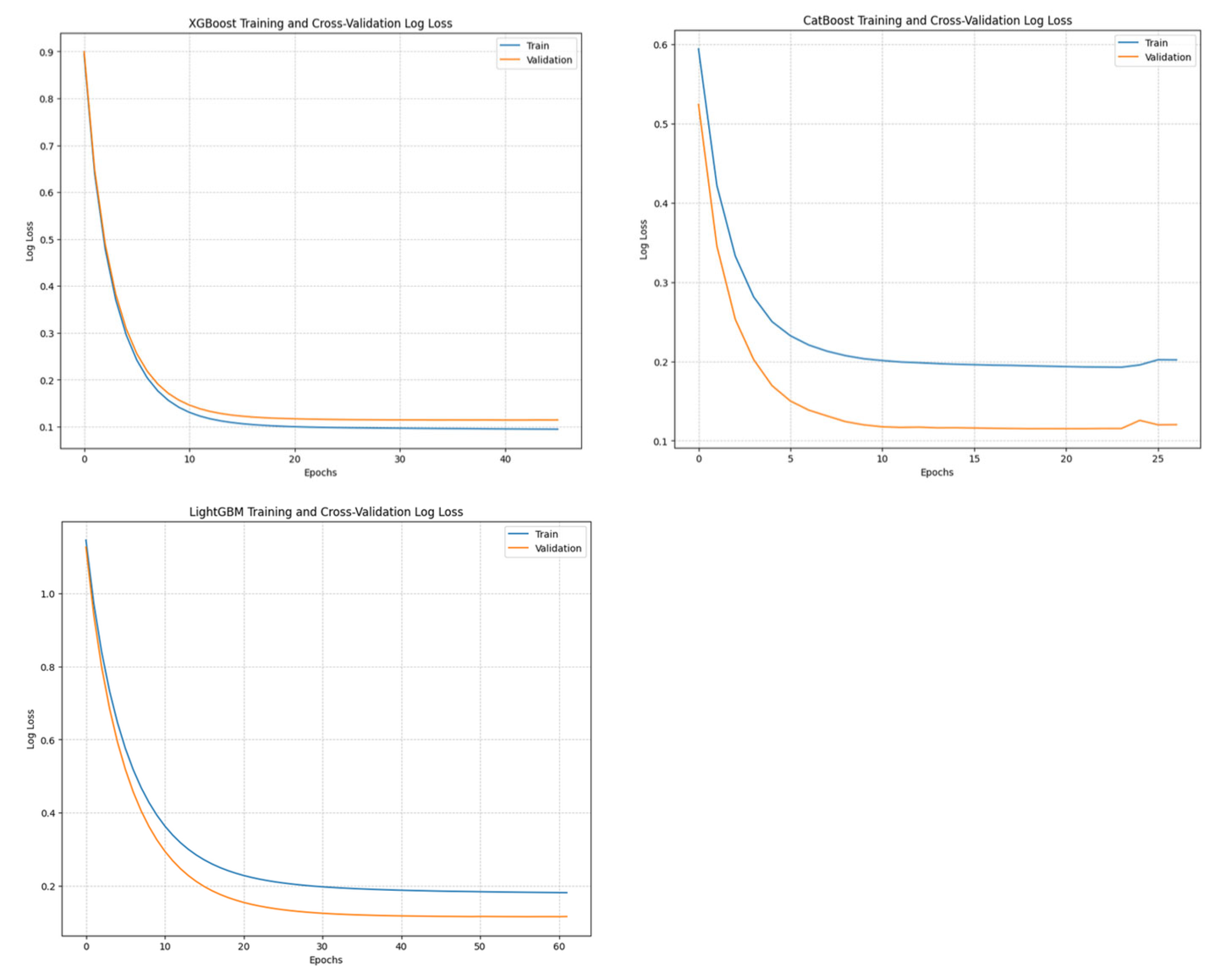
All models converged rapidly, with XGBoost models converging in fewer than 65 iterations. CatBoost and LightGBM showed good generalization, sometimes performing better on the validation set.

Best Hyperparameters:

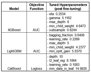
This Table shows the objective functions under which each model achieved optimal performance on the metrics, along with the best hyperparameter values identified during optimization using HyperOpt-TPE, which define the final models. AUC (Area Under ROC Curve). The name of the hyperparameters are shown as they are. Refer to Table 6 for the range of hyperparameter values explored as the search space for fine-tuning the different models.

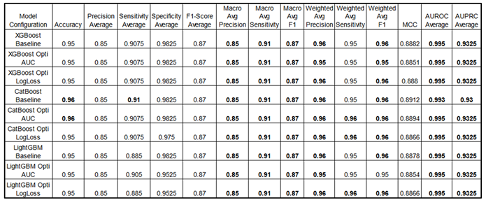
Performance Metrics :

The results below provide a performance benchmark for the best fine-tuned models. Notably, for all three GBMs, performance differences between each fine-tuned model and its respective baseline (default hyperparameters) were minimal, with metrics remaining closely aligned.

Some metrics are presented as averages, where "average" represents the mean result across all four classes for each metric, providing a streamlined overview (for detailed class-specific metrics, see the appendix part). Consistently high scores underscore the models' effectiveness in multi-class classification tasks. Optimization of objective functions (AUC and LogLoss) using the HyperOpt library yields slight performance gains, highlighting the impact of hyperparameter tuning. Optimized models are indicated with “Opti” as well as the objective function used for this goal. Note: Sensitivity is equivalent to Recall.

Feature Importance Analysis:

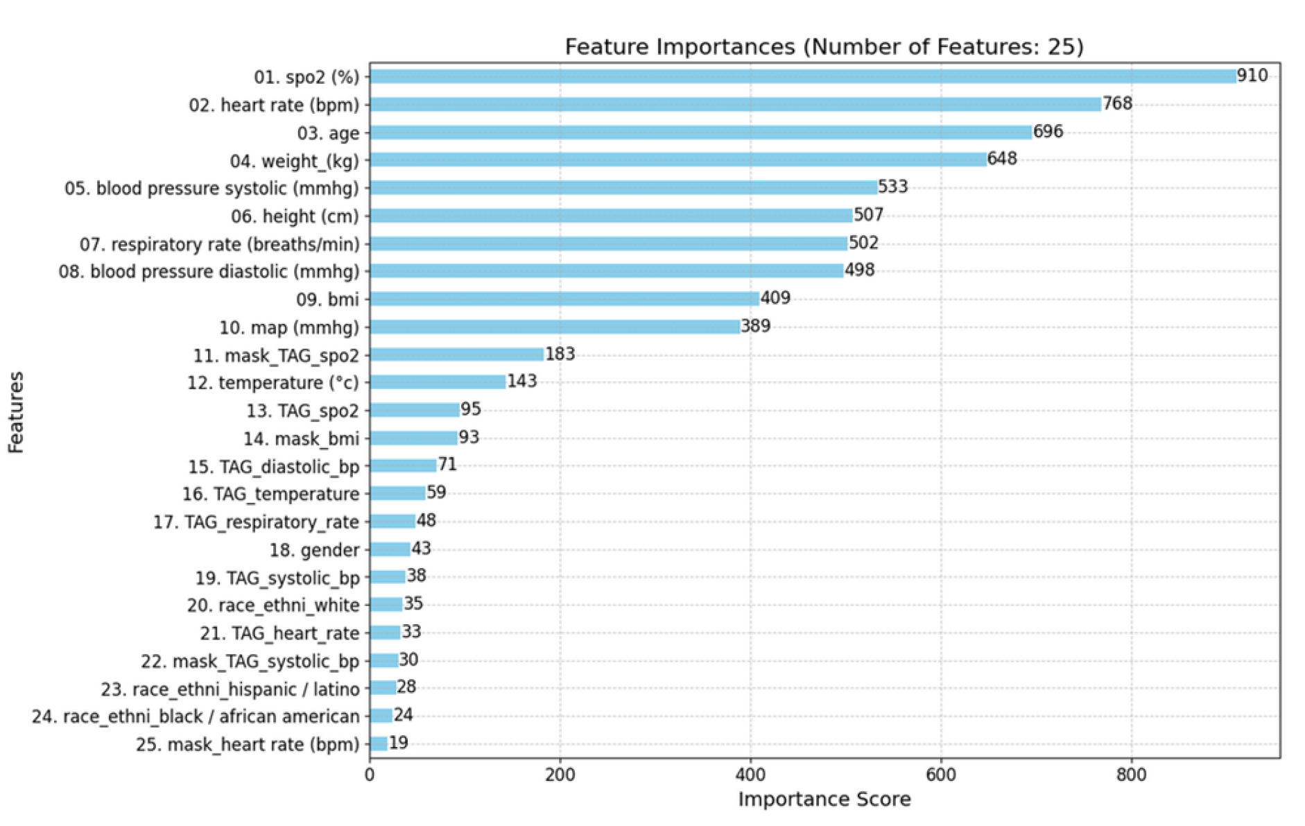
For XGBoost and LightGBM, both models considered a wide range of features, including physiological variables, TAGs, and mask features. The top contributing features were heart rate, systolic blood pressure, age, weight, and respiratory rate.

In contrast, CatBoost placed more emphasis on TAG features, with mask features being less significant. The top features in CatBoost included SpO₂, TAG SpO₂, height, age, and heart rate (see Figure 10).

Confusion Matrices:

The hypoxemia severity scores are the labels. Labels 2 and 3 were frequently misclassified, indicating challenges in predicting transitions between severity levels. Label 0 was most accurately predicted, followed by labels 3,1 and 2 (see label distribution, part 2.4). This aligns with the inherent challenge of predicting events that are both sudden and rare, such as the label "2." Importantly, this indicates that we can predict our primary complication, label 3, which corresponds to the most severe hypoxemic condition, with a reasonable degree of accuracy, supporting our proof of concept (POC).

3.4.2. Sequential Models' Results and Discussion

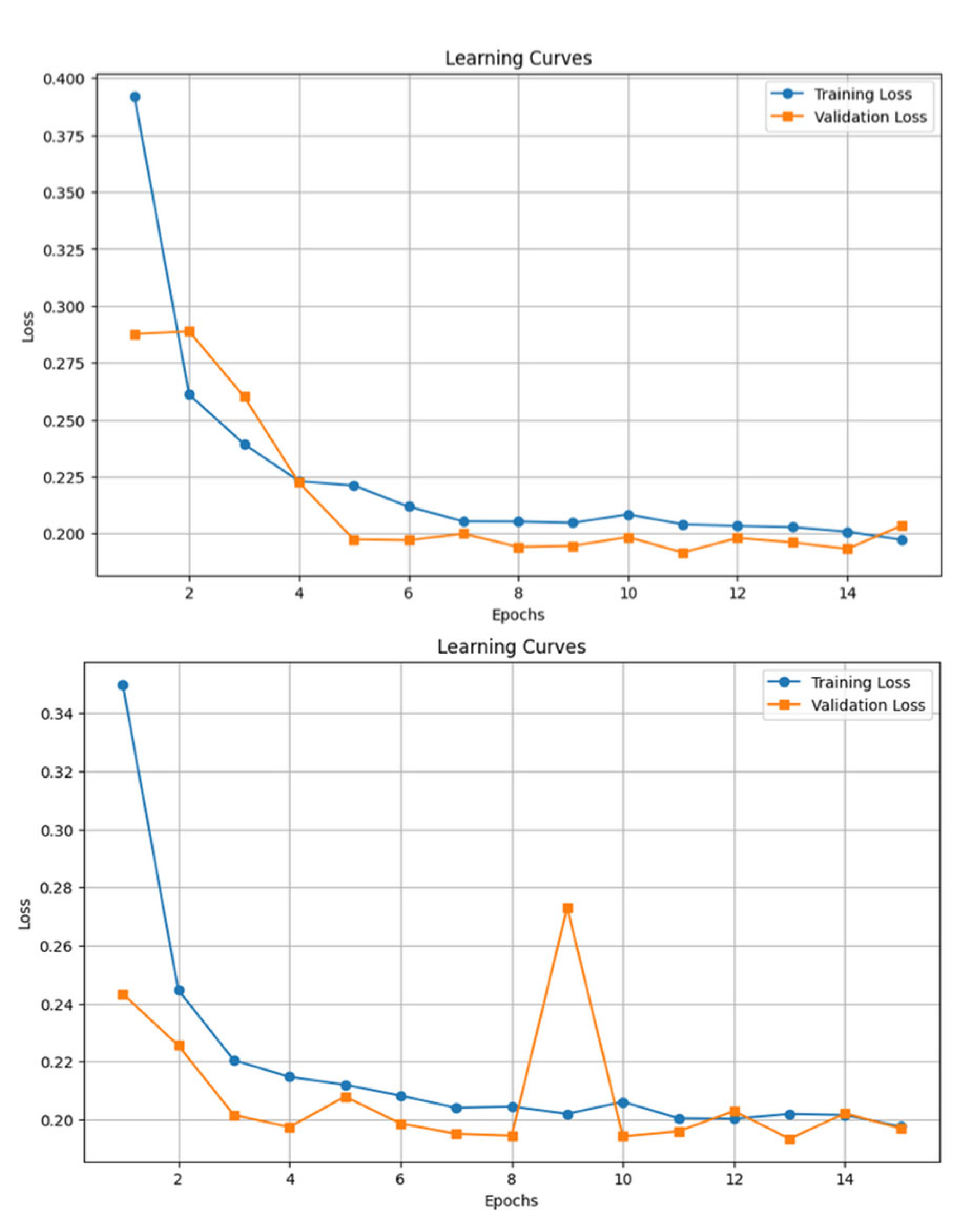
The LSTM and GRU models were trained using a 5-minute sliding window, with padding and masking applied to handle variable sequence lengths. By saving the models' parameters and hyperparameters at each epoch, we were able to reload the model from the optimal training epoch, ensuring the best performance was retained post-training.

Performance Metrics:

Table 11. Comparison of performance metrics for sequential models (LSTM and GRU) across various configurations.

Some metrics are presented as averages, where "average" denotes the mean result across all four classes, providing a concise overview (for detailed class-specific metrics, see the appendix). Consistently high scores highlight these models' effectiveness in multi-class classification tasks. Due to extensive training times, no fine-tuning was performed; instead, architectures with sufficient complexity were used as a proof of concept in this study. Note: Sensitivity is equivalent to Recall.

Training Time:

Training time was significantly longer than GBMs. Each training epoch took approximately 2.5 hours. Total training time was around 37.5 hours for each sequential model.

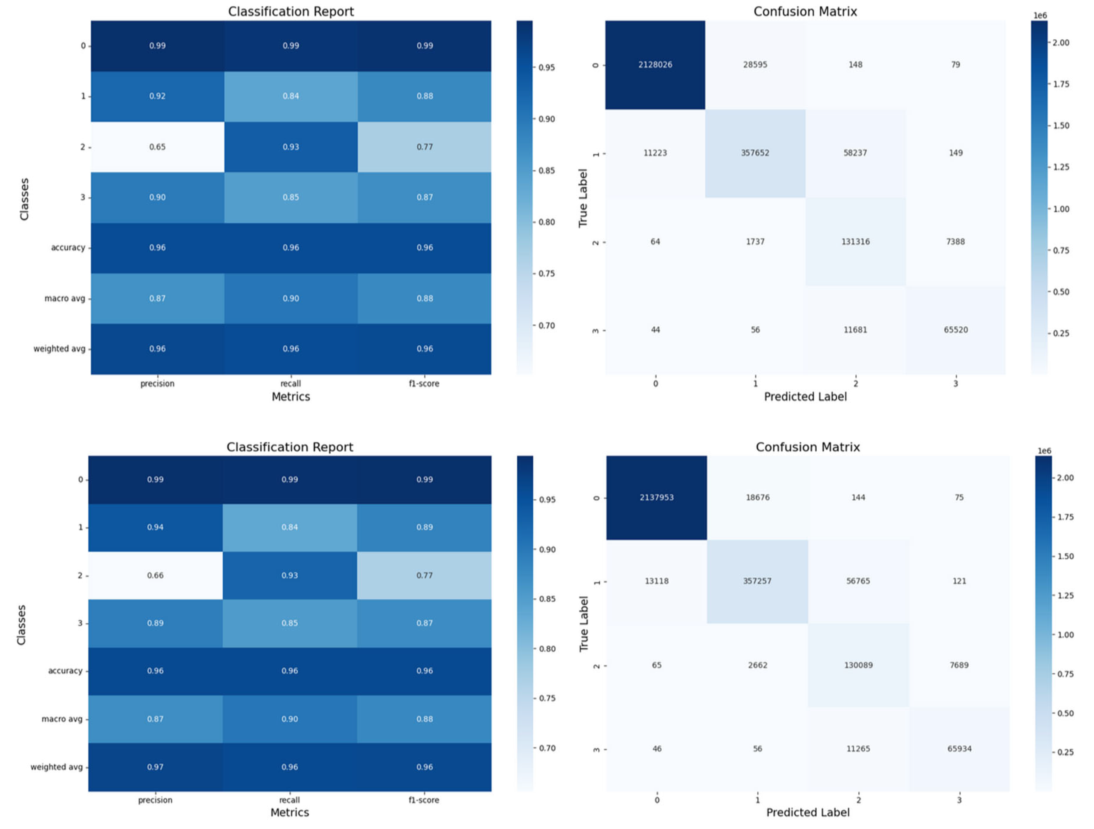
Figure 12. Confusion matrices and classification reports for LSTM and GRU models for the test set. The LSTM results are displayed at the top, and the GRU results at the bottom.

3.4.3. Comparison between GBMs and Sequential Models

While sequential models showed marginal improvements in some metrics, the gains did not justify the significantly longer training times and increased computational resources.

Concerning the Interpretability, GBMs offer greater transparency through feature importance metrics. For the Training Efficiency, GBMs trained much faster than sequential models (less than 3 minutes vs. 37.5 hours, per model). Finally, for the Performance Trade-offs, Sequential models performed slightly better in macro average F1 scores but were less practical for rapid deployment.

Performance Metrics:

The Table 12 provides a performance comparison between GBMs and sequential models. For a fairer assessment, we include the best fine-tuned GBM models optimized via HyperOpt TPE, alongside the performance results of the sequential models.

This table compares performance metrics for the best fine-tuned Gradient Boosting Models (XGBoost Opti AUC, CatBoost Opti AUC and LightGBM Opti LogLoss) and sequential models (LSTM, GRU) across configurations. Indeed, for a fair comparison, GBMs were optimized using HyperOpt TPE with objective functions like AUC and LogLoss, which provided slight performance gains and highlighted the value of hyperparameter tuning in general. Some metrics are shown as averages across all classes, providing a streamlined view (see appendix for detailed class metrics). Both GBM and sequential models consistently score high, demonstrating their effectiveness in multi-class classification tasks. Sequential models also perform well with a 5-minute sliding window approach, showing their suitability for time-series classification in general. Due to long training times, sequential models were not fine-tuned but used complex architectures as proof of concept. Note that decimal precision varies in reporting; for instance, Specificity Average for GRU is 0.9853, though this does not imply any advantage over models with fewer decimals. Both GBMs and sequential models deliver strong, competitive performance in multi-class classification but with pros and cons. See appendix A3 for all models’ comparison (including the baseline models).

3.5. Feature Importance and Model Interpretability

The feature importance rankings revealed that SpO₂ levels, heart rate, age, and respiratory rate were among the most significant predictors, which aligns well with clinical expectations. Notably, this analysis suggests clear patterns between SpO₂ and other physiological variables, supporting one of our hypotheses that patterns among features exist and are utilized by the model during training.

In focusing on the most important features for the gradient-boosting models (GBMs), we present the top 25 for clarity and interpretability. Both the XGBoost and LightGBM models underscored the importance of Mask Features, which differentiates between real and synthetic data derived from imputations and later interpolations, corroborating findings from previous studies [42,43,44,45]. Additionally, TAG score features consistently ranked quite highly across models, further affirming the utility of the NEWS2+ system in creating impactful, predictive features via its TAG scoring approach.

Although race and gender were less influential overall, they were still present among the top 25 features in some gradient-boosting models (GBMs). Their inclusion underscores the need for further investigation to ensure that any potential biases in model predictions are properly understood and managed.

4. Discussion

Our study demonstrates that machine learning models, particularly gradient boosting machines (GBMs), effectively predict hypoxemia severity using physiological parameters, among other factors. The strong performance of GBMs suggests that temporal data may not be essential for this prediction task. This aligns with findings from other studies indicating that deep learning models may not be ideal for tabular data, which, in our case, specifically takes the form of a time series [57].

Key Findings:

In comparing GBMs and sequential models, GBMs offer a practical balance of performance, interpretability, and training efficiency, while sequential models yield only slight performance gains at a much higher computational cost. Both types show strong, competitive performance in multi-class classification, though with different strengths and limitations. GBMs, while not designed to capture temporal dependencies, provide competitive results and train quickly, making them highly efficient. In contrast, sequential models, which consider temporal information, take significantly longer to train. For the purposes of this study, they were not fine-tuned due to time constraints, though further tuning might improve their performance.

In terms of feature importance, the inclusion of mask and TAG features notably improved model performance, emphasizing the value of transparent data preprocessing. Additionally, the TAG features derived from the NEWS2+ system demonstrated innovation, proving highly effective in enhancing model accuracy.

Regarding class imbalance, the class-weighted strategy allowed the models to handle the unbalanced dataset effectively, particularly in predicting the most severe hypoxemia cases (label 3). Even though label 1 was more prevalent, the models predicted label 3 more accurately, showcasing the success of the class-weighted approach.

The balance between sensitivity and specificity in model performance is challenging [28], especially for medical event predictions. High specificity with low sensitivity may reduce unnecessary interventions and related costs, as seen with D-dimer testing for venous thromboembolism [58], but could miss critical cases due to missing relevant variables or a limited number of outcome events, making such models more suited as a decision support tool rather than a stand-alone diagnostic tool. Conversely, high sensitivity with low specificity might capture non-specific patterns—such as variables associated with hypoxia but not exclusive to it—or detect subtle changes in nonhypoxic cases, leading to excessive false alerts and limiting clinical usability.

Limitations and Perspectives:

The data for this study was sourced from the MIMIC-III and IV databases, which may limit the generalizability of the findings. Our preprocessing involved minute-by-minute interpolation, but it is important to note that the data distribution from MIMIC-III and IV reflects a single hospital with no pediatric data (the minimum age post-preprocessing is 12-17 years). We also stratified patient ages into categories (see Table 4), but due to the dataset's lack of pediatric data and its imbalance across race and ethnicity categories, the model’s real deployment potential is limited with respect to these critical demographic factors.

Additionally, while the SpO₂/FiO₂ ratio (FiO₂ represents the Fraction of Inspired Oxygen in the inhaled gas), is a common indicator of respiratory distress in both clinical and pre-hospital settings (e.g., medical evacuation) [59,60], our study takes a different approach due to limitations in the available data. The MIMIC databases lack sufficient FiO₂ measurements, with a high proportion of values missing. Relying on the SpO₂/FiO₂ ratio would have introduced excessive uncertainty into the classification; instead, we prioritize SpO₂ measurements, which provide a more reliable basis for categorization. Imputing FiO₂ data to generate an SpO₂/FiO₂ ratio would have likely introduced further biases, especially in instances where both SpO₂ and FiO₂ values required imputation.

In terms of temporal information, sequential models (e.g., LSTM, GRU) did not demonstrate a significant performance advantage over GBMs, indicating that temporal dependencies may not be essential for predicting hypoxemia severity in this context. Nonetheless, to further validate our study, we should consider using a dataset with naturally regular intervals and fewer missing values, such as HiRID [61], which provides continuous physiological values recorded every two minutes, reducing the need for interpolation and imputation.

Implications for Practice:

GBMs can be integrated into systems like the VIMY Multi-System for real-time hypoxemia severity prediction, enabling rapid deployment in (pre)-clinical settings. Understanding the correlation between features and their importance is crucial for both model performance and interpretability. The feature importance metrics provide valuable insights for clinicians, aiding in the understanding of model decisions and improving trust and adoption, which ultimately enhances the interpretability of the system.

Additionally, we have a highly heterogeneous population, which is advantageous as our goal is to predict hypoxia in CBRNE situations in a broadly applicable, non-specific manner. A diverse population supports this aim, increasing the likelihood of developing a model with wide-ranging applicability.

Future Work:

Several key areas will be explored to enhance the performance and applicability of the models. First, data integration will focus on incorporating data from multiple hospital databases to improve the model's generalizability across diverse populations. The algorithms will then be tested prospectively on critically ill patients before being deployed in pre-clinical settings. Bias mitigation will ensure that the models remain free from biases related to race and gender, promoting fairness in outcomes. Lastly, real-time implementation will involve developing efficient algorithms suitable for deployment in resource-constrained environments, enabling timely and effective predictions in practical settings.

Fine-tuning the sequential models, despite the training time constraints, could likely bring even minor improvements, which in medical settings can be impactful. We also plan to test the recent xLSTM model, known for its efficiency and lighter architecture compared to other attention-based models, to assess its suitability in this context.

5. Conclusions

This study presents a proof of concept for using machine learning models to predict hypoxemia severity in (disaster) triage situations. The GBMs demonstrated robust performance and practicality for deployment within the VIMY Multi-System, while the sequential models, though theoretically advantageous for capturing temporal dependencies, provided marginal gains that did not justify the additional computational demands. Advanced feature engineering was conducted through our newly developed early warning system, NEWS2+, which generated feature scores (TAGs) for six primary physiological parameters. NEWS2+ also enabled the creation of SpO₂-based hypoxemia severity scores, adjusted for patient age and disease type, providing novel, clinically-informed labels tailored to our severity prediction task. Future work will emphasize enhancing model generalizability, integrating these models into real-time monitoring systems, and further supporting patient outcomes in emergency medical contexts.

List of Acronyms

SpO₂ : peripheral oxygen saturation.

LSTM: long short-term memory.

PPV: positive predictive value.

SaO2: arterial oxygen saturation.

GBT: gradient boosted tree.

AUROC: area under the receiver operating characteristics.

Lin: linear regression.

LR: logistic regression.

ANN: artificial neural network.

XGB: extreme gradient boosting.

RNN: recurrent neural network.

GBM: gradient boosting model.

PaO₂: partial pressure of oxygen.

FiO₂: fraction of oxygen in inhaled gas.

NN: neural network.

RF: random forest.

HR: heart rate.

BR: breath rate.

SBP: systolic blood pressure.

DBP: diastolic blood pressure.

AG: anion gap.

CNN: convolutional neural network.

MAE: mean averaged error to the range of values.

Supplementary Materials

The following supporting information can be downloaded at the website of this paper posted on Preprints.org, See the Appendix part. A1 Selected Pathologies in the admissions. A2. Inclusion diagram showing the main preprocessing steps before the imputations and interpolations (until point 12) and after (point 13-14). A3: Detailed comparison table of the performance metrics for Gradient Boosting Models (XGBoost, CatBoost, LightGBM) and Sequential Models (LSTM, GRU) under various configurations.

Author Contributions

Conceptualization: S.N.: M.A., A.W., P.J., S.B.; Data Curation: S.N., S.B.; Formal Analysis: S.N.; Funding Acquisition: M.A., P.J., S.B.; Investigation: S.N., Y.M., M.A., S.B.; Methodology: S.N., Y.M., M.A.; Project Administration: M.A., P.J., S.B.; Resources: M.A., P.J., S.B.; Software: S.N., Y.M.; Supervision: M.A., A.W., P.J., S.B.; Validation: S.N., Y.M., M.A.; Visualization: S.N., Y.M., M.A., A.W., P.J., S.B.; Writing – Original Draft: S.N., M.A.; Writing – Review & Editing: S.N., M.A., A.W., P.J. All authors have read and agreed to the published version of the manuscript.

Funding

This research was funded by Ivado's "Scientific in Action" program, through a consortium including the SADC-CDSS Lab of the CHU Sainte Justine Hospital in Montreal, Canada, applicare.ai Solutions inc, and Medint CBRNE Group consulting.

Institutional Review Board Statement

Not applicable.

Informed Consent Statement

Not applicable.

Data Availability Statement

The data supporting reported results were obtained from the MIMIC-III and MIMIC-IV databases, which are publicly available after an approval procedure at https://mimic.physionet.org/.

Acknowledgments

The authors express their sincere gratitude to the Clinical Decision Support Systems (CDSS) Lab at CHU Sainte-Justine in Montreal, the startup Solutions Applicare.ai, and the MEDINT CBRNE Group consulting for their invaluable support and collaboration. Special thanks go to former students Ons Loukil and Wala Bahri for their contributions to specific coding frameworks and their inspiring work. The authors also thank Professor Ioannis Mitliagkas from Mila/Université de Montréal for his administrative support.

Conflicts of Interest

The authors declare no conflicts of interest.

References

Baker, D.J. Critical Care Requirements after Mass Toxic Agent Release. Crit. Care Med. 2005, 33, S66–S74. [Google Scholar] [CrossRef] [PubMed]
Carli, P.; Telion, C.; Baker, D. Terrorism in France. Prehospital Disaster Med. 2003, 18, 92–99. [Google Scholar] [CrossRef] [PubMed]
Okumura, T.; Suzuki, K.; Fukuda, A.; Kohama, A.; Takasu, N.; Ishimatsu, S.; Hinohara, S. The Tokyo Subway Sarin Attack: Disaster Management, Part 1: Community Emergency Response*. Acad. Emerg. Med. 1998, 5, 613–617. [Google Scholar] [CrossRef] [PubMed]
Bourassa, S.; Paquette-Raynard, E.; Noebert, D.; Dauphin, M.; Akinola, P.S.; Marseilles, J.; Jouvet, P.; Leclerc, J. Gaps in Prehospital Care for Patients Exposed to a Chemical Attack – A Systematic Review. Prehospital Disaster Med. 2022, 37, 230–239. [Google Scholar] [CrossRef] [PubMed]
39e Congrès de La Recherche Au CHU Sainte-Justine : 5-6 Février 2025 Available online:. Available online: https://recherche.chusj.org/fr/congres2021 (accessed on 19 July 2024).
JQRSR 2021 – RSR du Québec.
Inc, M.I.C. Medint Cbrne Group- Groupe Medint Cbrne Available online:. Available online: https://medintcbrne.com/projects-%26-projets (accessed on 19 July 2024).
Bourassa, S. The Medical Management of Casualties in a Chemical Contaminated Environment : A Start for the CBRNE Defence Research Program for Clinicians. 2023.
Greenhalgh, T.; Treadwell, J.; Ms, R.B.; Roberts, N.; Tavare, A.; Pullyblank, A. Should We Use the NEWS (or NEWS2) Score When Assessing Patients with Possible COVID-19 in Primary Care? Additional Contributors (Topic Experts). 2020. [CrossRef]
Alam, N.; Vegting, I.L.; Houben, E.; van Berkel, B.; Vaughan, L.; Kramer, M.H.H.; Nanayakkara, P.W.B. Exploring the Performance of the National Early Warning Score (NEWS) in a European Emergency Department. Resuscitation 2015, 90, 111–115. [Google Scholar] [CrossRef]
Tavaré, A.; Pullyblank, A.; Redfern, E.; Collen, A.; Barker, R.O.; Gibson, A. NEWS2 in Out-of-Hospital Settings, the Ambulance and the Emergency Department. Clin. Med. 2022, 22, 525–529. [Google Scholar] [CrossRef]
National Early Warning Score (NEWS) 2 Available online:. Available online: https://www.rcp.ac.uk/improving-care/resources/national-early-warning-score-news-2/ (accessed on 24 October 2024).
Paediatric Early Warning Score (PEWS) Available online:. Available online: https://ihub.scot/improvement-programmes/scottish-patient-safety-programme-spsp/maternity-and-children-quality-improvement-collaborative-mcqic/paediatric-care/paediatric-early-warning-score-pews/ (accessed on 12 October 2023).
Paediatric Observation Reference Ranges for Referrers Available online:. Available online: https://www.clinicalguidelines.scot.nhs.uk/rhc-for-health-professionals/referring-a-patient/paediatric-observation-reference-ranges-for-referrers/ (accessed on 3 July 2024).
Akre, M.; Finkelstein, M.; Erickson, M.; Liu, M.; Vanderbilt, L.; Billman, G. Sensitivity of the Pediatric Early Warning Score to Identify Patient Deterioration. Pediatrics 2010, 125, e763–e769. [Google Scholar] [CrossRef]
Chapman, S.M.; Maconochie, I.K. Early Warning Scores in Paediatrics: An Overview. Arch. Dis. Child. 2019, 104, 395–399. [Google Scholar] [CrossRef]
Pediatric Vital Signs Normal Ranges | Iowa Head and Neck Protocols Available online:. Available online: https://medicine.uiowa.edu/iowaprotocols/pediatric-vital-signs-normal-ranges (accessed on 3 July 2024).
Flynn, J.T.; Kaelber, D.C.; Baker-Smith, C.M.; Blowey, D.; Carroll, A.E.; Daniels, S.R.; de Ferranti, S.D.; Dionne, J.M.; Falkner, B.; Flinn, S.K.; et al. Clinical Practice Guideline for Screening and Management of High Blood Pressure in Children and Adolescents. Pediatrics 2017, 140, e20171904. [Google Scholar] [CrossRef]
Validation of a Modified Early Warning Score in Medical Admissions. Available online: https://read.qxmd.com/read/11588210/validation-of-a-modified-early-warning-score-in-medical-admissions (accessed on 3 July 2024).
Khan, A.; Sarma, D.; Gowda, C.; Rodrigues, G. The Role of Modified Early Warning Score (MEWS) in the Prognosis of Acute Pancreatitis. Oman Med. J. 2021, 36, e272. [Google Scholar] [CrossRef]
Effect of Introducing the Modified Early Warning Score on Clinical Outcomes, Cardio-Pulmonary Arrests and Intensive Care Utilisation in Acute Medical Admissions. Available online: https://read.qxmd.com/read/12859475/effect-of-introducing-the-modified-early-warning-score-on-clinical-outcomes-cardio-pulmonary-arrests-and-intensive-care-utilisation-in-acute-medical-admissions (accessed on 3 July 2024).
Smith, M.E.B.; Chiovaro, J.C.; O’Neil, M.; Kansagara, D.; Quiñones, A.R.; Freeman, M.; Motu’apuaka, M.L.; Slatore, C.G. Early Warning System Scores for Clinical Deterioration in Hospitalized Patients: A Systematic Review. Ann. Am. Thorac. Soc. 2014, 11, 1454–1465. [Google Scholar] [CrossRef] [PubMed]
Gerry, S.; Bonnici, T.; Birks, J.; Kirtley, S.; Virdee, P.S.; Watkinson, P.J.; Collins, G.S. Early Warning Scores for Detecting Deterioration in Adult Hospital Patients: Systematic Review and Critical Appraisal of Methodology. BMJ 2020, 369, m1501. [Google Scholar] [CrossRef] [PubMed]
Downey, C.L.; Tahir, W.; Randell, R.; Brown, J.M.; Jayne, D.G. Strengths and Limitations of Early Warning Scores: A Systematic Review and Narrative Synthesis. Int. J. Nurs. Stud. 2017, 76, 106–119. [Google Scholar] [CrossRef] [PubMed]
Fu, L.-H.; Schwartz, J.; Moy, A.; Knaplund, C.; Kang, M.-J.; Schnock, K.O.; Garcia, J.P.; Jia, H.; Dykes, P.C.; Cato, K.; et al. Development and Validation of Early Warning Score System: A Systematic Literature Review. J. Biomed. Inform. 2020, 105, 103410. [Google Scholar] [CrossRef]
Shamout, F.E.; Zhu, T.; Sharma, P.; Watkinson, P.J.; Clifton, D.A. Deep Interpretable Early Warning System for the Detection of Clinical Deterioration. IEEE J. Biomed. Health Inform. 2020, 24, 437–446. [Google Scholar] [CrossRef]
Lauritsen, S.M.; Kristensen, M.; Olsen, M.V.; Larsen, M.S.; Lauritsen, K.M.; Jørgensen, M.J.; Lange, J.; Thiesson, B. Explainable Artificial Intelligence Model to Predict Acute Critical Illness from Electronic Health Records. Nat. Commun. 2020, 11, 3852. [Google Scholar] [CrossRef]
Pigat, L.; Geisler, B.P.; Sheikhalishahi, S.; Sander, J.; Kaspar, M.; Schmutz, M.; Rohr, S.O.; Wild, C.M.; Goss, S.; Zaghdoudi, S.; et al. Predicting Hypoxia Using Machine Learning: Systematic Review. JMIR Med. Inform. 2024, 12, e50642. [Google Scholar] [CrossRef]
Johnson, A.; Pollard, T.; Mark, R. MIMIC-III Clinical Database 2015.
Johnson, A.E.W.; Pollard, T.J.; Shen, L.; Lehman, L.H.; Feng, M.; Ghassemi, M.; Moody, B.; Szolovits, P.; Anthony Celi, L.; Mark, R.G. MIMIC-III, a Freely Accessible Critical Care Database. Sci. Data 2016, 3, 160035. [Google Scholar] [CrossRef]
Johnson, A.E.W.; Bulgarelli, L.; Shen, L.; Gayles, A.; Shammout, A.; Horng, S.; Pollard, T.J.; Hao, S.; Moody, B.; Gow, B.; et al. MIMIC-IV, a Freely Accessible Electronic Health Record Dataset. Sci. Data 2023, 10, 1. [Google Scholar] [CrossRef]
Ke, G.; Meng, Q.; Finley, T.; Wang, T.; Chen, W.; Ma, W.; Ye, Q.; Liu, T.-Y. LightGBM: A Highly Efficient Gradient Boosting Decision Tree. In Proceedings of the Advances in Neural Information Processing Systems; Curran Associates, Inc., 2017; Vol. 30. [Google Scholar]
Prokhorenkova, L.; Gusev, G.; Vorobev, A.; Dorogush, A.V.; Gulin, A. CatBoost: Unbiased Boosting with Categorical Features.
Chen, T.; Guestrin, C. XGBoost: A Scalable Tree Boosting System. In Proceedings of the Proceedings of the 22nd ACM SIGKDD International Conference on Knowledge Discovery and Data Mining; ACM: San Francisco California USA, August 13, 2016; pp. 785–794. [Google Scholar]
Gers, F.A.; Schmidhuber, J.; Cummins, F. Learning to Forget: Continual Prediction with LSTM. In Proceedings of the 1999 Ninth International Conference on Artificial Neural Networks ICANN 99. (Conf. Publ. No. 470); September 1999; Vol. 2; pp. 850–855. [Google Scholar]
Chung, J.; Gulcehre, C.; Cho, K.; Bengio, Y. Empirical Evaluation of Gated Recurrent Neural Networks on Sequence Modeling Available online:. Available online: https://arxiv.org/abs/1412.3555v1 (accessed on 20 July 2024).
Hochreiter, S.; Schmidhuber, J. Long Short-Term Memory. Neural Comput. 1997, 9, 1735–1780. [Google Scholar] [CrossRef]
Dempsey, J.A.; Wagner, P.D. Exercise-Induced Arterial Hypoxemia. J. Appl. Physiol. 1999, 87, 1997–2006. [Google Scholar] [CrossRef] [PubMed]
Johannigman, J.; Gerlach, T.; Cox, D.; Juhasz, J.; Britton, T.; Elterman, J.; Rodriquez, D.; Blakeman, T.; Branson, R. Hypoxemia during Aeromedical Evacuation of the Walking Wounded. J. Trauma Acute Care Surg. 2015, 79, S216–220. [Google Scholar] [CrossRef] [PubMed]
Bourassa, S.; Bouchard, P.-A.; Dauphin, M.; Lellouche, F. Oxygen Conservation Methods With Automated Titration. Respir. Care 2020, 65, 1433–1442. [Google Scholar] [CrossRef] [PubMed]
Samad, M.D.; Abrar, S.; Diawara, N. Missing Value Estimation Using Clustering and Deep Learning within Multiple Imputation Framework. Knowl.-Based Syst. 2022, 249, 108968. [Google Scholar] [CrossRef] [PubMed]
Perez-Lebel, A.; Varoquaux, G.; Le Morvan, M.; Josse, J.; Poline, J.-B. Benchmarking Missing-Values Approaches for Predictive Models on Health Databases. GigaScience 2022, 11, giac013. [Google Scholar] [CrossRef]
Josse, J.; Chen, J.M.; Prost, N.; Scornet, E.; Varoquaux, G. On the Consistency of Supervised Learning with Missing Values 2024.
Sharafoddini, A.; Dubin, J.A.; Maslove, D.M.; Lee, J. A New Insight Into Missing Data in Intensive Care Unit Patient Profiles: Observational Study. JMIR Med. Inform. 2019, 7, e11605. [Google Scholar] [CrossRef]
Sperrin, M.; Martin, G.P.; Sisk, R.; Peek, N. Missing Data Should Be Handled Differently for Prediction than for Description or Causal Explanation. J. Clin. Epidemiol. 2020, 125, 183–187. [Google Scholar] [CrossRef]
Kusters, R.; Misevic, D.; Berry, H.; Cully, A.; Le Cunff, Y.; Dandoy, L.; Díaz-Rodríguez, N.; Ficher, M.; Grizou, J.; Othmani, A.; et al. Interdisciplinary Research in Artificial Intelligence: Challenges and Opportunities. Front. Big Data 2020, 3. [Google Scholar] [CrossRef]
Lundberg, S.M.; Nair, B.; Vavilala, M.S.; Horibe, M.; Eisses, M.J.; Adams, T.; Liston, D.E.; Low, D.K.-W.; Newman, S.-F.; Kim, J.; et al. Explainable Machine-Learning Predictions for the Prevention of Hypoxaemia during Surgery. Nat. Biomed. Eng. 2018, 2, 749. [Google Scholar] [CrossRef]
Annapragada, A.V.; Greenstein, J.L.; Bose, S.N.; Winters, B.D.; Sarma, S.V.; Winslow, R.L. SWIFT: A Deep Learning Approach to Prediction of Hypoxemic Events in Critically-Ill Patients Using SpO2 Waveform Prediction. PLOS Comput. Biol. 2021, 17, e1009712. [Google Scholar] [CrossRef]
Bureau, U.C. About the Topic of Race Available online:. Available online: https://www.census.gov/topics/population/race/about.html (accessed on 15 July 2024).
Lassman, D.; Hartman, M.; Washington, B.; Andrews, K.; Catlin, A. US Health Spending Trends By Age And Gender: Selected Years 2002–10. Health Aff. (Millwood) 2014, 33, 815–822. [Google Scholar] [CrossRef] [PubMed]
González-Nóvoa, J.A.; Busto, L.; Rodríguez-Andina, J.J.; Fariña, J.; Segura, M.; Gómez, V.; Vila, D.; Veiga, C. Using Explainable Machine Learning to Improve Intensive Care Unit Alarm Systems. Sensors 2021, 21, 7125. [Google Scholar] [CrossRef]
Hyland, S.L.; Faltys, M.; Hüser, M.; Lyu, X.; Gumbsch, T.; Esteban, C.; Bock, C.; Horn, M.; Moor, M.; Rieck, B. Early Prediction of Circulatory Failure in the Intensive Care Unit Using Machine Learning. Nat. Med. 2020, 26, 364–373. [Google Scholar] [CrossRef]
Zheng, J.; Li, J.; Zhang, Z.; Yu, Y.; Tan, J.; Liu, Y.; Gong, J.; Wang, T.; Wu, X.; Guo, Z. Clinical Data Based XGBoost Algorithm for Infection Risk Prediction of Patients with Decompensated Cirrhosis: A 10-Year (2012–2021) Multicenter Retrospective Case-Control Study. BMC Gastroenterol. 2023, 23, 1–10. [Google Scholar] [CrossRef] [PubMed]
Zhao, H.; Ma, Z.; Sun, Y. Predict Onset Age of Hypertension Using CatBoost and Medical Big Data. In Proceedings of the 2020 International Conference on Networking and Network Applications (NaNA); December 2020; pp. 405–409. [Google Scholar]
Pham, T.D. Time–Frequency Time–Space LSTM for Robust Classification of Physiological Signals. Sci. Rep. 2021, 11, 6936. [Google Scholar] [CrossRef] [PubMed]
Lipton, Z.C.; Kale, D.C.; Elkan, C.; Wetzel, R. Learning to Diagnose with LSTM Recurrent Neural Networks 2017.
Shwartz-Ziv, R.; Armon, A. Tabular Data: Deep Learning Is Not All You Need 2021.
Weitz, J.I.; Fredenburgh, J.C.; Eikelboom, J.W. A Test in Context: D-Dimer. J. Am. Coll. Cardiol. 2017, 70, 2411–2420. [Google Scholar] [CrossRef]
Bouillon-Minois, J.-B.; Roux, V.; Jabaudon, M.; Flannery, M.; Duchenne, J.; Dumesnil, M.; Paillard-Turenne, M.; Gendre, P.-H.; Grapin, K.; Rieu, B.; et al. Impact of Air Transport on SpO2/FiO2 among Critical COVID-19 Patients during the First Pandemic Wave in France. J. Clin. Med. 2021, 10, 5223. [Google Scholar] [CrossRef]
Chen, W.; Janz, D.R.; Shaver, C.M.; Bernard, G.R.; Bastarache, J.A.; Ware, L.B. Clinical Characteristics and Outcomes Are Similar in ARDS Diagnosed by Oxygen Saturation/Fio2 Ratio Compared With Pao2/Fio2 Ratio. Chest 2015, 148, 1477–1483. [Google Scholar] [CrossRef]
Faltys, M.; Zimmermann, M.; Lyu, X.; Hüser, M.; Hyland, S.; Rätsch, G.; Merz, T. HiRID, a High Time-Resolution ICU Dataset.

Figure 1. An illustration that shows the VIMY Multisystem deployment [8], in a glance, during a medical response in a contaminated environment. Our goal is to develop a proof of concept for AI models that will ensure effective triage in CBRNE environments and other pre-clinical settings.

Figure 2. The illustration represents a simulated hypoxemia condition, testing the monitoring-scoring-treatment nexus through an iterative process [8]. 1. Monitoring: Continuous monitoring of vital signs provides real-time data on key physiological variables such as respiratory rate, temperature, blood pressure, heart rate, and SpO₂ (oxygen saturation). Both real and simulated data are analyzed to detect correlations and patterns in these digital biomarkers. This analysis helps in predicting the severity score of hypoxemia. 2. Scoring: Based on SpO₂ levels, a hypoxemia severity score is determined, ranging from 0 (best) to 3 (worst). This predicted severity score informs triage decisions, categorizing the patient's condition as Stat, Urgent, or Stable. 3. Treatment Administration: Depending on the severity score, appropriate treatments are administered. For instance, a patient with low oxygen saturation may receive oxygen therapy (with or without an oxygen mask) to stabilize their condition.

Figure 3. Simplified Inclusion diagram showing the main preprocessing steps before the imputations and interpolations, and after. See complete one in the appendix.

Figure 4. Labellisation process overview. Designed on a decision-tree like system. In our process, we have no children (patients < 18 years) with COPD, only without. For each of the three categories, we used different threshold values for SpO2 (%) to determine the severity scores.

Figure 5. Correlation matrix of main physiological variables before imputations and interpolations.

Figure 6. PCA variance explained and feature contributions. In green, the percentage of variance accounted for by each principal component is illustrated, and in blue, the cumulative variance of each PC added to those before.

Figure 7. Overview of Main Preprocessing Steps for Sequential Models with a 5-Minute Sliding Window Illustration for the Initial Minutes of an Admission.

Figure 8. Shift-lag illustration for a shift of -1 (for illustrative purposes). Observe the red arrows to see how each y label is moved one position backward (denoted as -1). The result : the label of each given row is the future severity in x-minutes. (Where label “Y” represents, in our case, the hypoxemia severity score).

Figure 9. Training curves of baseline models showing loss over iterations for the 5 min in advance predictions. XGBoost (left), CatBoost (middle) and LightGBM (right). XGBoost showed slight overfitting, while CatBoost and LightGBM generally demonstrated better generalization to the validation set compared to the training set. Given the overall good performance of all models, we concluded that they all learned effectively during training.

Figure 10. Top 25 Feature Importance derived from the GBMs for predicting hypoxemia score 5 minutes in advance: XGBoost (top left), CatBoost (top right), and LightGBM (bottom left). The models do not utilize the features in the same way when constructing their successive prediction trees. This discrepancy highlights the differences in how each model prioritizes and processes the various features to make predictions.

Figure 11. Training curves over epochs for LSTM (left) and GRU (right) models.

Table 1. NEWS2+ Scoring Matrices for Hypoxemia Severity by Patient Type.

Table 2. NEWS2+ Scoring Matrix: Feature Scores (TAGs) for Physiological Variables in Adults and Pediatric.

Table 3. Comparison of interpolation methods showing physiological variables' maximum range values after interpolation.

Table 4. Demographics of the study population after preprocessing.

Table 5. Label distribution of hypoxemia severity scores before and after interpolation.

Table 6. Default and tuned hyperparameters of the three gradient-boosting machine models (GBMs).

Table 7. Architecture and hyperparameters of the sequential models.

Table 8. Common feature columns used to train both GBMs and sequential models. Notice that there are also masks for the six different TAGs-score-features.

Table 9. Best fine-tuned models for each GBM following optimization.

Table 10. Comparison of performance metrics for the GBMs (XGBoost, CatBoost, and LightGBM models) across various configurations.

Table 12. Performance Comparison of Best Fine‐Tuned‐GBMs and the Sequential Models.

Disclaimer/Publisher’s Note: The statements, opinions and data contained in all publications are solely those of the individual author(s) and contributor(s) and not of MDPI and/or the editor(s). MDPI and/or the editor(s) disclaim responsibility for any injury to people or property resulting from any ideas, methods, instructions or products referred to in the content.

© 2024 by the authors. Licensee MDPI, Basel, Switzerland. This article is an open access article distributed under the terms and conditions of the Creative Commons Attribution (CC BY) license (http://creativecommons.org/licenses/by/4.0/).

Copyright: This open access article is published under a Creative Commons CC BY 4.0 license, which permit the free download, distribution, and reuse, provided that the author and preprint are cited in any reuse.

Alerts

MDPI Initiatives

Important Links

Choose an area of interest and we will send you notifications of new preprints at your preferred frequency.

Disclaimer