Preprint
Review

Genome Language Modeling (Glm): A Beginner’s Cheat Sheet

Altmetrics

Downloads

147

Views

121

Comments

0

This version is not peer-reviewed

Submitted:

04 November 2024

Posted:

05 November 2024

You are already at the latest version

Alerts
Abstract
Combining genomics with digital healthcare information is set to transform per- sonalized medicine. However, this integration is challenging due to the differing nature of the data modalities. The large size of the genome makes it impossible to store it as part of the standard electronic health record (EHR) system. Rep- resenting the genome as a condensed representation containing biomarkers and usable features is required to make the genome interoperable with EHR data. This systematic review examines both conventional and state-of-the-art methods for genome language modeling (GLM), which involves representing and extract- ing features from genomic sequences. Feature extraction is an essential step for applying machine learning (ML) models to large genomic datasets, especially within integrated workflows. We first provide a step-by-step guide to various genomic sequence pre-processing and representation techniques. Then we explore feature extraction methods including tokenization, and transformation of tokens using frequency, embedding, and neural network-based approaches. In the end, we discuss ML applications in genomics, focusing on classification, prediction, and language processing algorithms. Additionally, we explore the role of GLM in func- tional annotation, emphasizing how advanced ML models, such as Bidirectional encoder representations from transformers (BERT), enhance the interpretation of genomic data. To the best of our knowledge, we compile the first end-to-end analytic guide to convert complex genomic data into biologically interpretable information using GLM, thereby facilitating the development of novel data-driven hypotheses.
Keywords: 
Subject: Biology and Life Sciences  -   Biology and Biotechnology

1. Background

Natural Language Processing (NLP) is a sub-field of computer science and artificial intelligence (AI) focused on the interaction between computers and human languages. It allows computers to understand, interpret, and generate human language in a way that is meaningful to machines. NLP applications have evolved significantly over time, starting with foundational tasks and progressing to advanced technologies. Early applications included text classification, where algorithms categorized text into predefined labels, and machine translation, which converted text from one language to another. Sentiment analysis followed, enabling the extraction of emotional tone from text, and speech recognition, which transformed spoken language into written text. More advanced applications like named entity recognition (NER) and information retrieval emerged, focusing on extracting relevant entities and data from large text corpora. Language modeling techniques such as next sentence prediction (NSP), masked language modeling (MLM), and the development of large language models (LLMs) represent the latest advancements in NLP. These models are proving crucial for understanding, generating, and predicting natural language, and a wider use of such applications is gaining momentum.
Genomic information consists of DNA sequences encoding the genetic code and translating it into functional biomolecules such as RNA or protein. This information can be represented using four nucleotide alphabets (also known as bases) namely, A, T, G, and C as unstructured text. In recent years, NLP has found several applications in the field of genomics involving analyses using DNA/ RNA, or protein sequences, all of which can be represented as text. For example, NLP-based algorithms were used for protein sequence classification [2], for identifying DNA modification sites [26], functional annotations of co-expressed gene pairs [7], prediction of gene promoters [3], RNA modifications sites [32], enhancers [17], DNA replication origins [28], for generating pseudo nucleotide composition [5] or even representation of protein sequences [29].
The use of NLP techniques for genome language modeling (GLM) is appealing because genomic sequences can be processed in a manner similar to natural language text sequences. Therefore, GLM involves using NLP models to interpret and predict genetic sequences, treating them as a "language" with its own syntax and semantics. This approach enables the development of models that can identify and predict genetic features, enhancing our understanding of biological grammar. However, the grammar it follows and the distinctions of genomic “words” are not as apparent. Despite these challenges, this innovative approach enables the development of models that can identify and predict genetic features and enhance our understanding of biological grammar by using sequence data alone.
GLM represents a significant advancement in computational biology by applying NLP techniques to uncover insights from complex biological data. By applying GLM, researchers can develop more accurate predictive models, improve functional annotations, and gain a deeper understanding of the underlying mechanisms of gene expression and regulation. In this review, we will present an overview of the current opportunities and challenges in the field of GLM. Additionally, we will discuss the methods and demonstrate typical workflows used in GLM. Where possible, we will provide a comparative analysis of algorithms. While we will use DNA sequences as our example data to illustrate different methodologies, these same methods can also be applied to other types of biological sequence data, such as RNA or protein sequences.

2. Main Text

GLM Workflow of Genomic Sequence Analysis

In this section, we provide an overview of a typical workflow of GLM that involves genomic sequence analysis using ML techniques. The workflow includes steps such as genomics sequence representation, feature extraction methods, ML applications, and functional annotation. These methods are crucial for understanding how raw genomic data can be transformed into meaningful insights through NLP methods.

2.1. Genomic Sequence Representation

Representing genomic sequences is an essential aspect of GLM. This involves converting DNA sequences, represented by A, C, G, and T characters, (and RNA sequences, in which T is replaced by U character) into numerical forms. Sequence representation involves two main steps. First, preprocessing larger sequences into smaller units to work upon. The second step is encoding these sequences where text sub-units are converted into numerical formats suitable for computational analysis.

2.1.1. Preprocessing

Before numerical encoding, biological sequence data often undergoes preprocessing steps to enhance quality and usability. Common preprocessing techniques include:
a. Due to the extensive length of DNA sequences, which can range from hundreds to hundreds of millions of base pairs (bp), preprocessing involves segmenting these sequences into smaller, manageable chunks. This step is essential to reduce computational costs and enable downstream algorithms to efficiently process and analyze relevant sub-sequences [Figure 1].
b. Data cleaning: Filtering out common genomic terms or sequences containing little or unusable information, such as the character ‘N’ in nucleotide sequence data [Figure 1].
c. Normalization: Standardizing sequences to a uniform format, addressing variations like case sensitivity or character encoding.

2.1.2. Sequence Encoding Techniques

Sequence encoding in GLM has evolved significantly, starting with fundamental encoding techniques such as ordinal encoding [19], where nucleotides are encoded as integers based on their alphabetical order (e.g., A = 1, C = 2, G = 3, T = 4) [Figure 1]. This method simplifies the representation of sequences into numerical values but may not capture underlying relationships between nucleotides. Another popular encoding method is one-hot encoding, which maps each nucleotide (A, C, G, T) to a binary vector representation [Figure 1]. In this scheme, each nucleotide is represented as a vector of zeros with a single one indicating its presence (e.g., A = [1, 0, 0, 0], C = [0, 1, 0, 0], etc.). Beyond these foundational methods, other historical encoding techniques include sum, Helmert, polynomial, and binary encoding [19]. These methods aimed to capture more nuanced relationships between categorical values, providing alternatives to simple one-hot or ordinal representations. For instance, sum encoding represents each category by its deviation from the grand mean. In contrast, Helmert’s encoding contrasts each level of a categorical variable with the mean of the subsequent levels. Even though this article focuses more on nucleotide sequences (DNA/RNA), the same approach can be applied to protein sequences that are written using 20 alphabets known as amino acid characters.

2.2. Feature Extraction

Feature extraction is the next vital step in subsequent analysis and modeling that involves the preprocessing and encoding steps we introduced earlier.

2.2.1. Tokenization

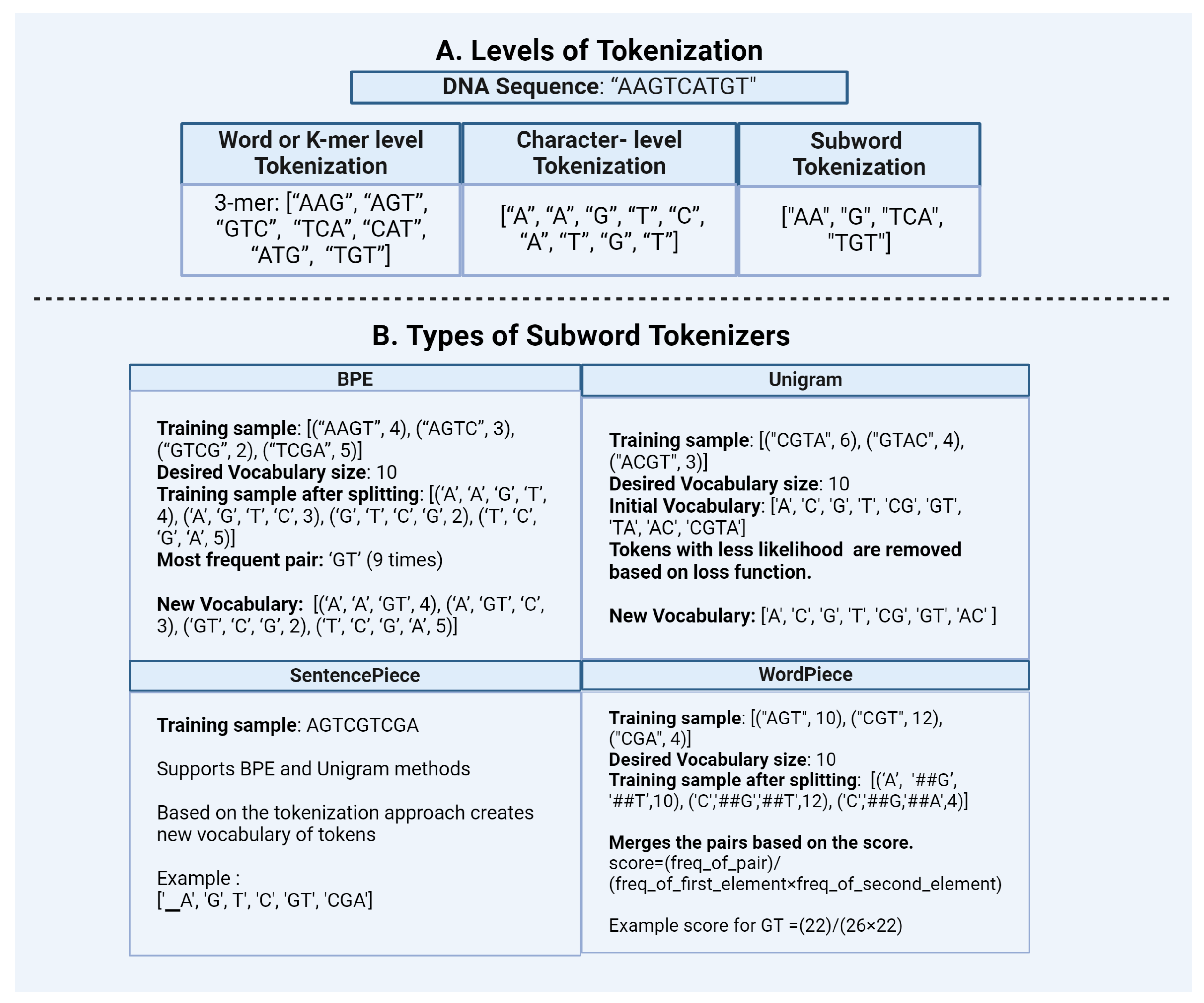
In the preprocessing step, tokenization involves breaking down long DNA, RNA, or protein sequences into smaller units called tokens. These tokens serve as the basic building blocks for subsequent analysis [Figure 2].

1. Word or K-Mer Level:

In the context of biological sequences, k-mer is a sub-sequence of k length (e.g. 3-mers and 4-mers). K-mers are generated by shifting an overlapping window of size k throughout the sequence. This is equivalent to ‘words’ of human language. Large amounts of data can be easily tokenized by this method. Since we generate all overlapping k-mers of a given length, the resulting number of tokens is very high, leading to a high computational cost. The determination of values of "k" is ad-hoc and is usually based on guesswork [Figure 2]. Another drawback of this type of tokenization method is that they do not accommodate Out-of-vocabulary (OOV) words. OOV words are words that are absent from the vocabulary of a language model or tokenizer. These words may include misspellings, rare words, or domain-specific terms not encountered during model training. Additionally, this approach fails to capture the semantic relationship between the tokens, limiting its effectiveness in understanding the context and meaning of sequences.

2. Character Level:

This tokenization method splits the sequences into individual characters, effectively handling OOV words by breaking them into their component characters. This results in a significantly smaller vocabulary size, as it includes only the four nucleotide characters (A, T, G, C). However, this approach loses semantic relationships between tokens, as the context and meaning derived from longer sequences are not captured. Additionally, while the vocabulary size is reduced compared to the word or K-mer level tokenization, the overall length of the tokenized sequence increases, making the process non-reversible and less efficient for capturing higher-level features [Figure 2].

3. Subword Tokenization:

Subword tokenization divides sequences into smaller units or subwords. N-grams, sequences of n tokens, are commonly used. The most frequent words receive unique IDs, while the less frequent words are split into subwords. This approach addresses the drawbacks of word and character-level tokenization, such as large vocabulary sizes, inability to handle OOV tokens, and increased sequence lengths, by breaking them into known subwords. It also maintains the semantic relationships between tokens. Typically, subword tokenizers use pre-tokenized input rather than raw data [Figure 2].

3.1 Byte Pair Encoding (BPE)

BPE is a compression algorithm i.e. it encodes or compresses data and is widely used in NLP pipelines to perform subword tokenization. It addresses the drawbacks of Word and Character Tokenization as it handles OOV tokens and has a limited vocabulary size. Vocabulary size of BPE can be a user-defined parameter. Initially, the vocabulary consists of unique characters or subwords of various lengths from the tokens in the training sample along with their respective frequencies. The tokens in the training sample are first split into individual characters from the vocabulary. These characters represent the smallest units of the words. The algorithm then identifies the most frequent combinations of adjacent characters, sub-words, or multi-character sequences and merges them to form new subwords. This process is repeated iteratively, with the most frequent sequences being merged at each step, gradually building up more complex subwords until the entire vocabulary is either compressed to the desired size or fully merged[Figure 2]. However, since BPE implements simple merging rule based on the most frequent tokens, it does not account for semantics of the tokens which can result in non-meaningful subwords. This leads to sub-optimal tokenization. BPE is employed in language models like GPT-2, XLM, and FlauBERT.

3.2 Unigram

The unigram model solves the merging problem of BPE by calculating the likelihood of each subword combination rather than picking the most frequent pattern. Initial vocabulary of unigram consists of different combinations of tokens created by the frequency or BPE-based approach. Subword tokens with the highest losses are removed from this vocabulary at each iteration step until the desired vocabulary size is achieved [Figure 2].This ensures that the model retains subwords that are not only frequent but also meaningful. Unigram approach is usually used in conjunction with SentencePiece in popular architectures such as BigBird and XLNet.

3.3 Specialized subword tokenizer

  • SentencePiece: SentencePiece is a modified version of subword units approach. It is an effective and language-independent sub-word tokenizer, owing to its pre-tokenization-free approach. During tokenization, SentencePiece treats the sentences as raw texts and defines a fixed vocabulary size for creating the vocabulary. It then converts all characters into Unicode including whitespaces. This feature helps to handle accurate reverse conversion from detokenized tokens to original ones (lossless tokenization). Using these features, SentencePiece could be easily extended to languages like Japanese and Chinese, which do not use spaces. This feature makes it an effective approach for biological sequences as well. SentencePiece also gives flexibility to choose between BPE and Unigram as subword algorithms which improves the robustness of the entire tokenization approach [Figure 2]. Transformer models like ALBERT, XLNet, and T5 use SentencePiece in conjunction with Unigram.
  • WordPiece: WordPiece is a tokenization approach similar to BPE. It has similar merge rules like BPE but differs in the selection of token pairs to be merged. WordPiece starts by creating a vocabulary of tokens from the initial words by splitting the word into each character and appending WordPiece prefix ’##’. It then merges the tokens based on the below scoring formula. According to this formula, the pairs which appear less frequently in the text gets merged than those which appear too frequently. WordPiece was developed by Google to train the BERT model, then it got reused in many other transformer models like DistilBERT, MobileBERT and MPNET.
score = freq_of_pair freq_of_first_element × req_of_second_element

2.2.2. Transforming Tokens Using Frequency-Based Representation

Tokens generated from tokenization are required to be encoded as numerical values and transformed as either vectors or multi-dimensional matrices before feeding them into learning algorithms to design models. Traditional methods of transforming tokens include ordinal encoding, one-hot encoding, and other encoding methods discussed in the earlier section. This section explores frequency-based representation methods for the transformation of tokens.
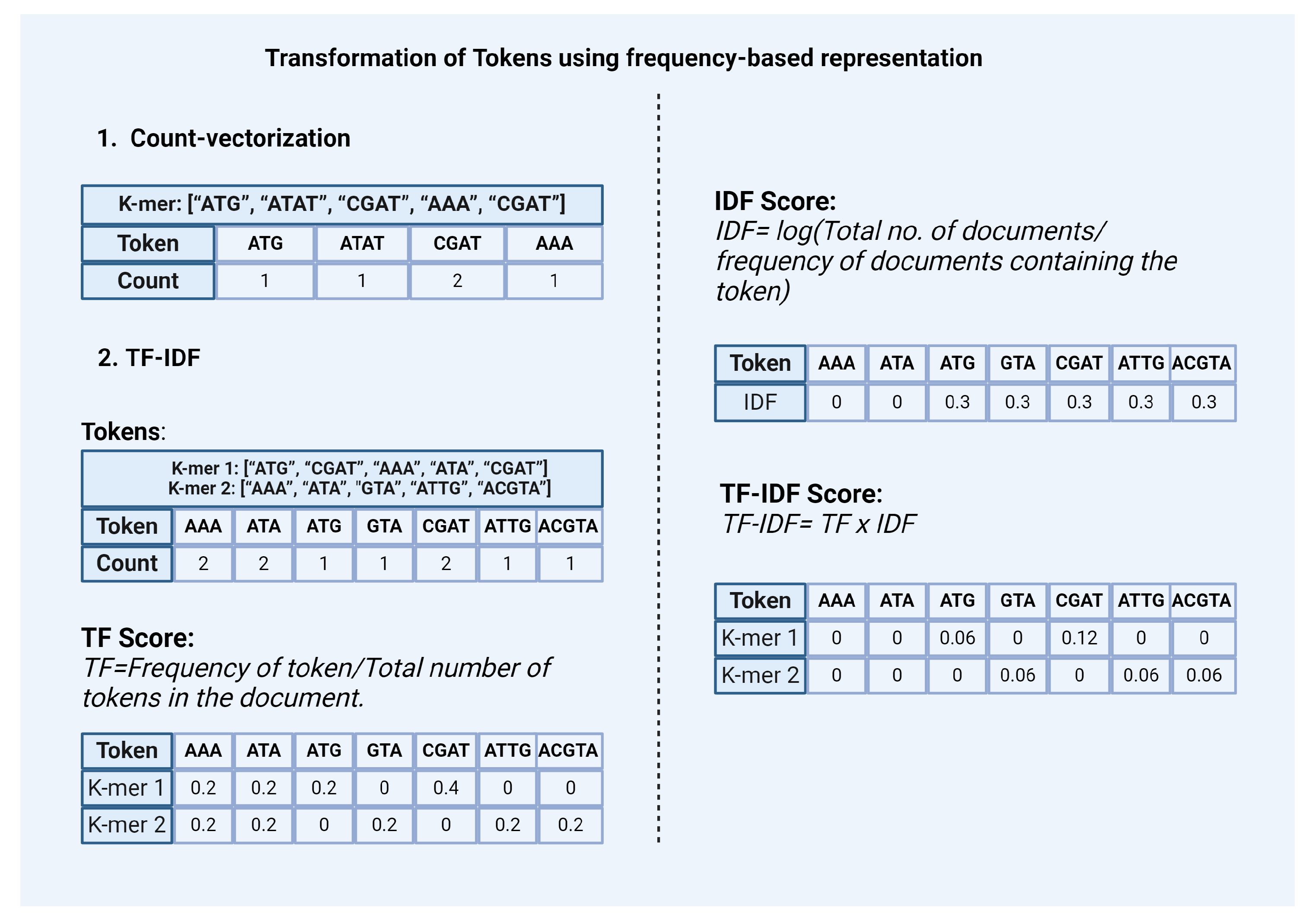
  • Count-vectorization: This method counts the number of occurrences of each token and represents it as a vector or matrix [Figure 3]. This method considers high-frequency words as more significant.
  • TF-IDF: In the context of natural language data Term Frequency-Inverse Document Frequency (TF-IDF) is a statistic based on the frequency of a token in the document. It is used to analyze the difference between the two documents by the uniqueness of tokens. A higher value of TF-IDF signifies higher importance of the tokens in the corpus while lower values represent lower importance. It is calculated by combining two metrics: Term Frequency (TF) and Inverse Document Frequency (IDF) [Figure 3].
    Term Frequency (TF) score
    It is based on the frequency of tokens or words in the document. TF is calculated by dividing the number of occurrences of a token (i) by the total number (N) of tokens in the document (j).
    TF (i) = frequency (i,j) / N (j)
    Inverse Document Frequency (IDF) score
    It is a measure that indicates how commonly a token is used. It can be calculated by dividing the total number (N) of documents (d) by the number of documents containing the token (i).
    IDF (i) = log (N (d) / frequency (d, i))
    The final TF-IDF score is calculated by multiplying TF and IDF scores.
    TF-IDF (i) = TF (i) x IDF (i)
    Similar to the Countvectorizer method, TF-IDF also gives priority to the tokens that have the highest frequency of occurrence in the document or the corpus. However, these count-based methods fail to capture the semantic relationship between tokens.

2.2.3. Transforming Tokens Using Embedding and Neural Network-Based Representations

More recently, embeddings and neural network-based have been used for token transformations. Embedding is a learned transformation for corpus where we compare tokens by comparing features to find relationships between them. Each token is mapped to one vector. Similar tokens have a representation identical to vectors/matrices. The distributed representation is learned based on their usage. This allows tokens used in similar ways to have similar representations, naturally capturing their relation. We have classified the embedding models into two broad categories:

Non-Contextual

Non-contextual representation is short-ranged. It just converts each token into one vector without considering the context in which they are used. Two same tokens will have the same representation disregarding their different semantic meanings. Two common algorithms in this category are Word2vec and Glove.
1.
Word2Vec
Word2Vec is a statistical method that attempts to explain word embedding based on the corpus. It can do that by implementing two strategies:
  • Continuous Bag-of-Words, or CBOW model.
  • Continuous Skip-Gram Model.
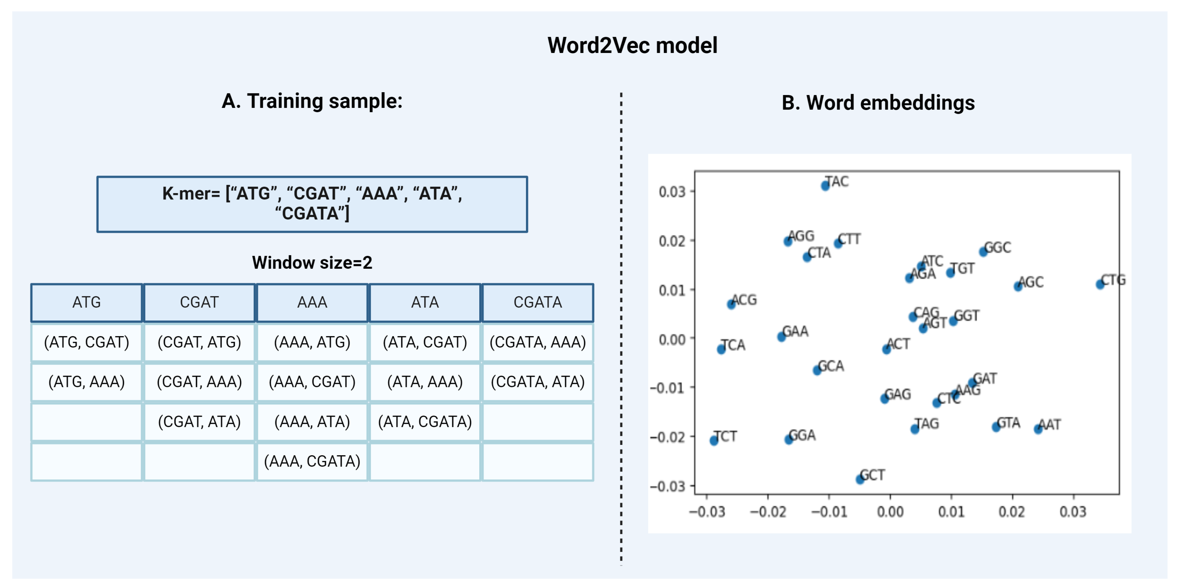
CBOW is a representation of text that describes the occurrence of words within a document. This model is only concerned with whether known words occur in the document, not where in the document. We convert a corpus of text of variable-length (unstructured data) into a fixed-length vector which is structured and well-defined and thus preferred by NLP Algorithms. The CBOW model learns the embedding by predicting the current word based on its semantics or context. The continuous skip-gram model on the other hand, learns by predicting the surrounding words given a current word. Both models are focused on learning about words given their local usage context, where the context is defined by a predefined window of neighboring words. For Example, a window size of 2, means that for every word, we’ll consider the 2 words behind and the 2 words after it [Figure 4]. The Skip-Gram model works well with small-scale data, and better represents rare words or phrases. However, the CBOW model trains faster than Skip-Gram and better represents high-frequency words, thus giving a slightly better accuracy. The key benefit of the approach is that high-quality word embeddings can be learned efficiently i.e. with low space and time complexity, allowing larger embeddings to be learned from large-scale data. DNA2vec is the DNA equivalent of Word2vec i.e. it is used specifically for applying the Word2vec approach to DNA sequences. It is used to transform tokens of variable length k-mers preferably 3 to 8 using the skip-gram model approach and thus captures efficient information of the sequences [18]. Another example is the kmer2vec model which is more focused on embedding fixed-length k-mers, typically between 3 to 6 to capture sequence relationships. This model is useful for tasks that require uniform k-mer lengths such as identifying specific patterns within genomic sequences [21].
2.
Global Vectors for Word Representation (GloVe)
The GloVe model is an extension of the Word2vec model for efficiently learning word vectors. Word2Vec only captures the local context of words. GloVe considers the entire corpus and creates a large matrix from the words in the corpus. The matrix has the words as the rows and their occurrence frequency as the columns for a corpus of text. For large matrices, we factorize the matrix to create a smaller matrix. GloVe combines the advantages of two-word vector learning methods: matrix factorization and local context window methods like Skip-gram which reduces the computational cost of training the model. The resulting word embeddings are different and improved. Word tokens with similar semantic meanings or similar contexts are placed together, for example, ‘queen’ and ‘women’. Being an extension to Word2vec, GloVe can be used for the representation of biological sequences as well. In a recent study, the GloVe model was integrated into a hybrid machine-learning model to classify gene mutations in cancer [1].

Contextual

  • Embeddings from Language Models (ELMo)
    ELMo are another way to convert a corpus of text into vectors or embeddings. ELMo word vectors are calculated by using a two-layer bidirectional language (biLM) model. Each layer has 2 passes, a forward pass, and a backward pass. It first converts the words into vectors. These vectors act as inputs to the first layer of the biLM model. The forward pass extracts and stores the information about the word in vector form and the context before it. The backward pass extracts and stores the information about the word and the context (other words) after it. This information contributes to the formation of intermediate word vectors which act as an input to the second layer of biLM. The final representation is done by the weighted sum of the initial word vectors and the two intermediate word vectors formed by the two layers. Recent studies use ELMo-based models to create embeddings for downstream tasks like protein structure prediction [9] [23].
  • Transformers
    Transformers are a type of neural network architecture used for NLP tasks. Transformers make use of an attention mechanism i.e. when a transformer looks at a piece of data, like a DNA sequence, it doesn’t just focus on one part. It pays attention to all the different parts at the same time. This helps it understand how everything fits together and find important patterns or relationships between tokens in the corpus of data for generating embeddings. A transformer model uses self-attention mechanisms to relate different positions within a single sequence. This allows each position in the sequence to attend to all other positions in the sequence, enabling the model to capture contextual information more effectively than traditional models.
    BERT
    BERT rely on this attention mechanism. In contrast to traditional (uni)directional models that read sequences from either the left or the right, transformers, including BERT use a bidirectional approach by using MLM in which tokens are masked at different intervals and models use preceding and succeeding tokens to predict the hidden tokens. BERT is an encoder-only transformer model. It takes input sequences and transforms them into fixed-size representations that capture important features. Word2vec or GloVe models generate a single-word embedding representation for each word in the vocabulary, whereas BERT will form a contextualized embedding that takes into account the context for each occurrence of a given word and will be different for each word according to the sentence. This enables BERT to provide more nuanced and accurate representations. This feature can be useful for tasks like classification and understanding genomic sequences that can have messages read in both directions and function via both short and long-range interactions. In genomics, DNABERT is a specialized adaptation of BERT for DNA sequences [11]. It is pre-trained on short sections of genomic data, learning patterns, and relationships. A newer version of DNABERT, DNABERT-2, uses BPE and other techniques to improve performance [33]. GenomicBERT uses unigram empirical tokenization to handle longer genomic sequences effectively and BERT attention mechanism to capture contextual relationships across large-scale biological datasets [4]. Other models like BioBERT, focusing on biomedical literature are leveraged to extract meaningful information from a vast biomedical text corpus [13,30]. Similarly, ClinicalBERT is employed in medical decision-making by analyzing clinical notes [10].
    Generative Pre-trained Transformers (GPT)
    GPT are a type of transformer model but follows a different architecture than BERT. GPT models are based on a decoder-only framework. A decoder takes the representations generated from an encoder and uses these to generate predictions. GPT is trained using tasks like Autoregressive Language Modelling (ALM), where the model sees a series of sequences and predicts the next sequence. It will be suitable for tasks involving sequence prediction and understanding directional sequences in genomics. Numerous models inspired by GPT such as DNAGPT [31], BioGPT [15], GeneGPT [12], and ScGPT [6], are being pre-trained on genomic sequences and biomedical literature. These models are then employed in various specialised tasks like gene sequence recognition and protein sequence prediction. For example, DNAGPT has been specifically designed for DNA sequence tasks, while BioGPT focuses on generating biomedical text that can be adapted for genomic applications.
Table 1. Algorithms comparison: This table presents a detailed comparison of different encoding algorithms including ordinal encoding, one-hot encoding, word embedding, and BERT.
Aspect Ordinal Encoding One-hot encoding Word embedding BERT
Encoding form Each token is assigned an integer value. Each token is represented by a vector (matrix). Tokens that have the same meaning have similar representations. Each token is represented by real-valued vectors. BERT provides contextualized embedding by taking into account the context of each token occurrence.
Semantic relationship Does not capture the relationship between tokens. Does not capture the relationship between tokens. Captures the relationship between tokens. It captures the relationship between tokens.
Categorical variables preferred Suitable for ordinal variables but not for nominal. Suitable for both nominal and ordinal variables. Suitable for both nominal and ordinal variables. Suitable for both nominal and ordinal variables.
Memory consumption and training time Lower memory usage but may not scale well with large datasets. High memory consumption due to large dimensions. More efficient in terms of memory than one-hot encoding. High memory consumption but scales with more data for better accuracy.
Handling OOV (Out of Vocabulary) words Can not handle OOV words. Can not handle OOV words. Struggles with OOV words. Efficiently handles OOV words with the help of modern tokenizers.
Table 2. Overview of Tokenization Types.
Tokenization Approach Method Pros Cons Reversibility
Character Tokenization Splits the data into a set of characters. Handles OOV words by breaking them into characters. Also, it has a limited size of vocabulary since it contains only a unique set of characters. It doesn’t capture the semantic relationship between the tokens. Non-reversible
Word Tokenization Splits the data into tokens using a certain delimiter. Large amounts of text can be easily tokenized without using complex computation. Fails at handling Out of Vocabulary (OOV) words. Furthermore, doesn’t scale well with big datasets as it generates a huge amount of vocabulary. Reversible
K-mer based Tokenization The data is split into fragments of desired k-length. Computationally less expensive method to generate tokens for genomic sequences. Does not capture the relationship between the tokens and generates a larger vocabulary. Non-reversible
Subword Tokenization Splits the data into subwords (or n-gram characters). The most frequently used tokens are given unique IDs and the less frequent tokens are split into subwords. Transformer-based models use this algorithm for preparing vocabulary. Has a decent vocabulary size. It does capture the semantic relationship between the tokens. Increases computational cost while reducing the model interpretability. Non-reversible
Table 3. Overview of Sub-word Tokenization Techniques.
Method name Type of Model Feature
Byte pair encoding (BPE) Frequency-based Initially developed as a compression algorithm, found applicability in sub-word tokenization using frequency-based merge rules.
WordPiece Score-based Select tokens based on a scoring mechanism to create an effective tokenizer model.
Unigram Probability and loss function based By quantifying a loss function, iteratively removes less efficient tokens from a larger vocabulary based on their probabilities to build a fixed size vocabulary.
SentencePiece Data-driven tokenization Does not require pre-tokenization and is language independent. Provides flexible integration with BPE, Wordpiece, and Unigram methods

ML Applications in Genomics

ML has significantly transformed genomics, offering powerful tools and methods for a range of applications. In this section, we explore the primary applications of ML in genomics, including classification, prediction, and language generation.

1. Classification

ML techniques have been instrumental in classification tasks such as identifying gene expressions, categorizing cell types, protein classification, and distinguishing between healthy and diseased tissues. Techniques like Random Forest (RF), Word2Vec, and Convolutional Neural Network (CNN) have been widely used. For example, CNN was used to identify N4-methylcytosine sites in DNA sequences, demonstrating the effectiveness of deep learning algorithms in genomic data analysis [26]. Similarly, Word2Vec-based models such as Bio2Vec and Prot2Vec were used to classify protein sequences. These embeddings helped capture the sequences’ semantic relationship, improving classification accuracy [2]. In another case, word embeddings combined with a deep learning framework were used to identify DNA replication origins [28]. This approach showcases the effectiveness of deep learning algorithms in handling complex classification tasks in genomics.

2. Prediction

Predictive modeling in genomics focuses on forecasting genomic outcomes based on biological data. Techniques such as regression models, Recurrent Neural Networks (RNNs), and Long Short-Term Memory (LSTM) Networks are commonly used.
For example, a Residual Fully Connected Neural Network (RFCN) was employed for predicting gene regulatory networks [14]. Similarly, CNN and RF models were used to compare ML and DL approaches in promoter prediction across various species [3]. In another paper, LSTM and CNN models were used to predict RNA modifications using one-hot encoding, word embedding, and RGloVe, showcasing the versatility of neural network models in handling diverse genomic data types [27].

3. Language Generation

GLMs, particularly transformer-based models like BERT and GPT are apt at generating new sequences of nucleotides or amino acids that conform to the grammar and structure of the genetic code. These models leverage NLP techniques to capture genomic data’s contextual relationships.
Genomic sequences exhibit a time series like property where nucleotides (A, C, G, T) or amino acids are organized into meaningful units whose meaning is dependent on their context. These units can range from kmers and genes to larger genomic regions. GLMs are designed to capture this hierarchy, allowing for the generation of sequences that incorporate the genomic context.
GLMs consider the surrounding nucleotides or amino acids to accurately predict the next element in the sequence [22]. This contextual awareness is essential for generating biologically plausible sequences that align with the rules of the genetic code.
GLMs utilize various language modeling techniques to represent and generate nucleotide or amino acid sequences [24]. One prominent approach is ALM used by GPTs, which predicts the next token (nucleotide or amino acid) in a sequence based on the preceding tokens [20]. This technique allows GLMs to generate novel genomic sequences and aid in tasks such as sequence completion, mutation prediction, or identifying regulatory regions within genomes. These capabilities highlight the versatility and potential impact of applying language modeling to genomics.

Functional Annotation

Functional annotation is an important process in genomics that involves identifying and assigning biological information to raw sequences and their products. This process helps in understanding the functional elements of a genome, such as genes or proteins, and their roles in biological processes and pathways.
Historically, tools like BLAST (Basic Local Alignment Search Tool) were used to perform sequence similarity searches to infer functional information based on the similarity of the unknown sequence to the known sequences. BLAST identifies regions of local similarity between sequences and aligns them to determine the likelihood of functional and evolutionary relationships. This approach, while effective, is limited by its dependency on existing annotations and its linear, non-contextual nature [8]. This method often needs to be revised when dealing with novel sequences or those with low similarity to known genes.
In the context of ML, functional annotation can be enhanced by both rule-based and DL approaches in an alignment-free manner [25]. Rule-based models are interpretable and can report features that are important for a predicted outcome. These models are built on predefined rules and statistical correlations, making it straightforward to understand which features contribute to a specific prediction. For instance, identifying DNA modification sites using rule-based algorithms can yield easily interpretable results, allowing researchers to directly correlate specific nucleotide patterns with functional annotations [26].
DL models, such as those based on transformers, offer a more complex but powerful approach to functional annotation. These models can automatically learn intricate patterns in genomic data, providing insights that might be missed by rule-based methods. For example, BERT and other transformer models can generate attention scores that highlight which parts of the input sequence are most influential for a given prediction. These attention scores can then be mapped back to biological functions, helping to assign biological relevance to important features.
In genomics, attention mechanisms within transformer models have been used to predict enhancers, promoters, and other regulatory elements by identifying key sequence motifs and their interactions [7]. Similarly, specialized approaches like DNABERT and genomicBERT focus on DNA sequences, offering more precise annotations by leveraging the bidirectional nature of BERT to capture context from both directions in the sequence [11].
NSP in BERT models enhances function annotation by understanding the relationship between genetic elements. In identifying operons or polycistronic messages in prokaryotic genomes, NSP can help predict whether a sequence of genes is likely to be transcribed together, revealing functional units within the genome. For instance, in a study of bacterial genomes, NSP was used to predict operon structures, significantly improving the accuracy of functional annotations compared to traditional methods. By analyzing the sequence context, NSP can identify co-regulating genes, providing insights into their collective biological functions [16].
Overall, combining rule-based and deep learning methods provides a robust framework for functional annotation, enhancing our ability to decipher complex genomic information.

3. Conclusion

The application of NLP techniques in genomics, particularly through GLM, offers significant advancements in identifying, understanding, and predicting biological functions by using the sequence information alone. This interdisciplinary approach leverages the strengths of NLP to process and interpret genomic sequences as natural language, enabling new possibilities for research and medical applications.
One of the most promising applications of GLM is in personalised medicines. By training models on combined healthcare and genomic data, researchers can identify genetic markers associated with physiological and lifestyle factors. This will enhance robust prediction of susceptibility to various diseases. For instance, deep learning models can analyze patterns in DNA sequences associated with genetic disorders, potentially leading to early diagnosis and personalized treatment plans. BERT-based models have shown great potential in identifying disease-related gene expressions and mutations, offering insights that can guide clinical decision-making [32].
GLM also plays a critical role in functional genomics, where understanding gene function and regulation is paramount. The ability to accurately annotate genes and regulatory elements helps in constructing detailed maps of genetic interactions and pathways. These annotations are crucial for elucidating the mechanisms of gene expression and regulation, which can lead to the discovery of new therapeutic targets.
While the future of GLM in genomics is promising, there are significant limitations. Training on a variety of large-scale genomic datasets is computationally demanding, requiring substantial processing power and time. Like other ML approaches, class imbalance in genomic datasets also presents a challenge, as rare sequences might get overlooked, potentially biasing predictions. The lack of standardized benchmarks in new sequencing projects will pose a critical challenge for evaluating the outcomes of language models. Understanding how language models generate predictions in genomics is often more challenging than in natural language tasks, as the complete ’grammar’ and ’vocabulary’ of the genome are still being uncovered. For this reason, the risk of model hallucination, where the model produces information that doesn’t accurately reflect the underlying data, is especially concerning in genomics.
With these limitations in mind, future research in GLM may focus on developing more efficient models for the processing of large-scale genomic data while ensuring interpretability and validation benchmarks. GLM offers enormous potential for understanding genetic information and improving health outcomes. By addressing challenges and continuing to innovate, we can achieve significant achievements in genomic research and healthcare.

4. List of Abbreviations

  • EHR: Electronic Health Record
  • GLM: Genome Language Modeling
  • ML: Machine Learning
  • BERT: Bidirectional encoder representations from transformers
  • NLP: Natural Language Processing
  • NER: Named Entity Recognition
  • NSP: Next Sentence Prediction
  • MLM: Masked Language Modeling
  • LLMs: Large Language Models
  • DNA: Deoxyribonucleic acid
  • RNA: Ribonucleic acid
  • OOV: Out-of-vocabulary
  • BPE: Byte Pair Encoding
  • TF-IDF: Term Frequency-Inverse Document Frequency
  • CBOW: Continuous Bag-of-Words
  • GloVe: Global Vectors for Word Representation
  • ELMo: Embeddings from Language Models
  • biLM: bidirectional Language Model
  • GPT: Generative Pre-trained Transformers
  • ALM: Autoregressive Language Modelling
  • RF: Random Forest
  • CNN: Convolutional Neural Network
  • RNNs: Recurrent Neural Networks
  • LSTM: Long Short-Term Memory
  • RFCN: Residual Fully Connected Neural Network
  • BLAST: Basic Local Alignment Search Tool

5. Declarations

  • Funding: S.T acknowledges AISRF EMCR fellowship from Australian Academy of Science. N.V acknowledges scholarship (RRITFS and STEM) from RMIT University, Melbourne. N.T acknowledges APBioNet for the support to present GLM research at the International Conference on Bioinformatics (INCOB) 2023 in Australia.
  • Competing interests: The authors declare that they have no competing interests
  • Acknowledgements: We thank Tyrone Chen for helpful discussions and advise on the content.
  • Authors’ contributions: N.T.:Writing-Original Draft Preparation N.V.:Writing- Reviewing and Editing S.T.:Conceptualization, Methodology, Writing- Original draft preparation, Writing- Reviewing and Editing, Supervision.
  • Ethics approval and consent to participate: ’Not applicable’
  • Consent for publication: ’Not applicable’
  • Availability of data and materials: ’Not applicable’
  • Clinical trial number: ’Not Applicable’
Table 4. Supplementary table: Sequence processing methods.
Method name Method type Tokenizer strategy Language restriction Reversibility Application
Conventional word splitting Rule-based tokenization Separates words based on space and/or punctuation. Space-separated languages True Natural Language
Conventional sentence splitting Rule-based tokenization Separates sentences based on full stops. Full-stop separated languages True Natural Language
Penn TreeBank Rule-based tokenization Separates contracted words. Use of contracted words in the language True Natural Language
TweetTokeniser Rule-based tokenization Separates audio streams in the form of string into small tokens based on space and/or punctuation. Space-separated languages False Natural Language
MWET (Multi-Word Expression) Rule-based tokenization Processes tokenized set and merges MWE into single tokens. Needs predefined tokens. True Natural Language
TextBlob Rule-based tokenization Separates text into tokens based on space, punctuation, and/or tabs. None True Natural Language
spaCy Rule-based tokenization Separates text(various languages) into words based on space. Space-separated languages True Natural Language
GenSim Rule-based tokenization Separates text based on space and/or punctuation. Contracted words True Natural Language
Keras tokenizer Rule-based tokenization Separates text into integer sequence or vector that has a coefficient for each token None False Natural Language
Moses Rule-based tokenization Separates text based on spaces. Space-separated languages True Natural Language
MeCab Sequence segmentation Segments sentences into their parts of speech. None False Natural Language
KyTea Sequence segmentation Segments sentences into their parts of speech and pronunciation tags. None False Natural Language
Byte Pair Encoding (BPE) Sequence segmentation (requires pre-tokenized input) Recodes sequences into a standardized format by frequency. None False Natural Language
Wordpiece Sequence segmentation (requires pre-tokenized input) Recodes sequences into a standardized format by likelihood. Variant of BPE None False Natural Language
Unigram Sequence segmentation (requires pre-tokenized input) Recodes sequences into a standardized format by likelihood, producing a set of tokens and their probabilities. Variant of BPE None False Natural Language
SentencePiece Data-driven tokenization Empirically derives tokens by sequence segmentation with BPE or its variants i.e. WordPiece, Unigram. None True Natural Language
k-mers Rule-based tokenization Sequence data is split into tokens of fixed length None False Biology
Khmer Rule-based tokenization Sequences are arbitrarily split into subsequences. None False Biology
Tab Rule-based tokenization Separates text based on tabs between them. Tab-separated text True Natural Language

References

  1. Aburass S, Dorgham O, Al Shaqsi J (2024) A hybrid machine learning model for classifying gene mutations in cancer using lstm, bilstm, cnn, gru, and glove. Systems and Soft Computing 6:200110.
  2. Asgari E, Mofrad MR (2015) Continuous distributed representation of biological sequences for deep proteomics and genomics. PloS one 10(11):e0141287.
  3. Bhandari N, Khare S, Walambe R, et al (2021) Comparison of machine learning and deep learning techniques in promoter prediction across diverse species. PeerJ Computer Science 7:e365.
  4. Chen T, Tyagi N, Chauhan S, et al (2023) genomicbert and data-free deep-learning model evaluation. bioRxiv pp 2023–05.
  5. Chen W, Lei TY, Jin DC, et al (2014) Pseknc: a flexible web server for generating pseudo k-tuple nucleotide composition. Analytical biochemistry 456:53–60.
  6. Cui H, Wang C, Maan H, et al (2024) scgpt: toward building a foundation model for single-cell multi-omics using generative ai. Nature Methods pp 1–11.
  7. Du J, Jia P, Dai Y, et al (2019) Gene2vec: distributed representation of genes based on co-expression. BMC genomics 20:7–15.
  8. Ejigu GF, Jung J (2020) Review on the computational genome annotation of sequences obtained by next-generation sequencing. Biology 9(9):295.
  9. Heinzinger M, Elnaggar A, Wang Y, et al (2019) Modeling aspects of the language of life through transfer-learning protein sequences. BMC bioinformatics 20:1–17.
  10. Huang K, Altosaar J, Ranganath R (2019) Clinicalbert: Modeling clinical notes and predicting hospital readmission. arXiv preprint arXiv:190405342.
  11. Ji Y, Zhou Z, Liu H, et al (2021) Dnabert: pre-trained bidirectional encoder representations from transformers model for dna-language in genome. Bioinformatics 37(15):2112–2120.
  12. Jin Q, Yang Y, Chen Q, et al (2024) Genegpt: Augmenting large language models with domain tools for improved access to biomedical information. Bioinformatics 40(2):btae075.
  13. Lee J, Yoon W, Kim S, et al (2020) Biobert: a pre-trained biomedical language representation model for biomedical text mining. Bioinformatics 36(4):1234–1240.
  14. Liu D, Xu C, He W, et al (2021) Autogenome: an automl tool for genomic research. Artificial Intelligence in the Life Sciences 1:100017.
  15. Luo R, Sun L, Xia Y, et al (2022) Biogpt: generative pre-trained transformer for biomedical text generation and mining. Briefings in bioinformatics 23(6):bbac409.
  16. Mao Y, Zhang L, Zhang Z, et al (2019) Operon identification by combining cluster analysis, genetic algorithms, and next sentence prediction models. Nucleic Acids Research 47(13):e85.
  17. Mu X, Wang Y, Duan M, et al (2021) A novel position-specific encoding algorithm (seqpose) of nucleotide sequences and its application for detecting enhancers. International Journal of Molecular Sciences 22(6):3079.
  18. Ng P (2017) dna2vec: Consistent vector representations of variable-length k-mers. arXiv preprint arXiv:170106279.
  19. Potdar K, Pardawala TS, Pai CD (2017) A comparative study of categorical variable encoding techniques for neural network classifiers. International journal of computer applications 175(4):7–9.
  20. Pourmirzaei M, Esmaili F, Pourmirzaei M, et al (2024) Prot2token: A multi-task framework for protein language processing using autoregressive language modeling. bioRxiv pp 2024–05.
  21. Ren R, Yin C, S.-T. Yau S (2022) kmer2vec: A novel method for comparing dna sequences by word2vec embedding. Journal of Computational Biology 29(9):1001–1021.
  22. Sanabria M, Hirsch J, Joubert PM, et al (2024) Dna language model grover learns sequence context in the human genome. Nature Machine Intelligence pp 1–13.
  23. Sharma S, Daniel Jr R (2019) Bioflair: Pretrained pooled contextualized embeddings for biomedical sequence labeling tasks. arXiv preprint arXiv:190805760.
  24. Tahmid MT, Shahgir HS, Mahbub S, et al (2024) Birna-bert allows efficient rna language modeling with adaptive tokenization. bioRxiv pp 2024–07.
  25. Wade KE, Chen L, Deng C, et al (2024) Investigating alignment-free machine learning methods for HIV-1 subtype classification. Bioinformatics Advances 4(1):vbae108. https://doi.org/#1, URL https://doi.org/10.1093/bioadv/vbae108.
  26. Wahab A, Tayara H, Xuan Z, et al (2021) Dna sequences performs as natural language processing by exploiting deep learning algorithm for the identification of n4-methylcytosine. Scientific reports 11(1):212.
  27. Wang H, Liu H, Huang T, et al (2022) Emdlp: Ensemble multiscale deep learning model for rna methylation site prediction. BMC bioinformatics 23(1):221.
  28. Wu F, Yang R, Zhang C, et al (2021) A deep learning framework combined with word embedding to identify dna replication origins. Scientific reports 11(1):844.
  29. Yang KK, Wu Z, Bedbrook CN, et al (2018) Learned protein embeddings for machine learning. Bioinformatics 34(15):2642–2648.
  30. Yu X, Hu W, Lu S, et al (2019) Biobert based named entity recognition in electronic medical record. In: 2019 10th international conference on information technology in medicine and education (ITME), IEEE, pp 49–52.
  31. Zhang D, Zhang W, He B, et al (2023) Dnagpt: a generalized pretrained tool for multiple dna sequence analysis tasks. bioRxiv pp 2023–07.
  32. Zhang L, Li G, Li X, et al (2021) Edlm6apred: ensemble deep learning approach for mrna m6a site prediction. BMC bioinformatics 22(1):288.
  33. Zhou Z, Ji Y, Li W, et al (2023) Dnabert-2: Efficient foundation model and benchmark for multi-species genome. arXiv preprint arXiv:230615006.
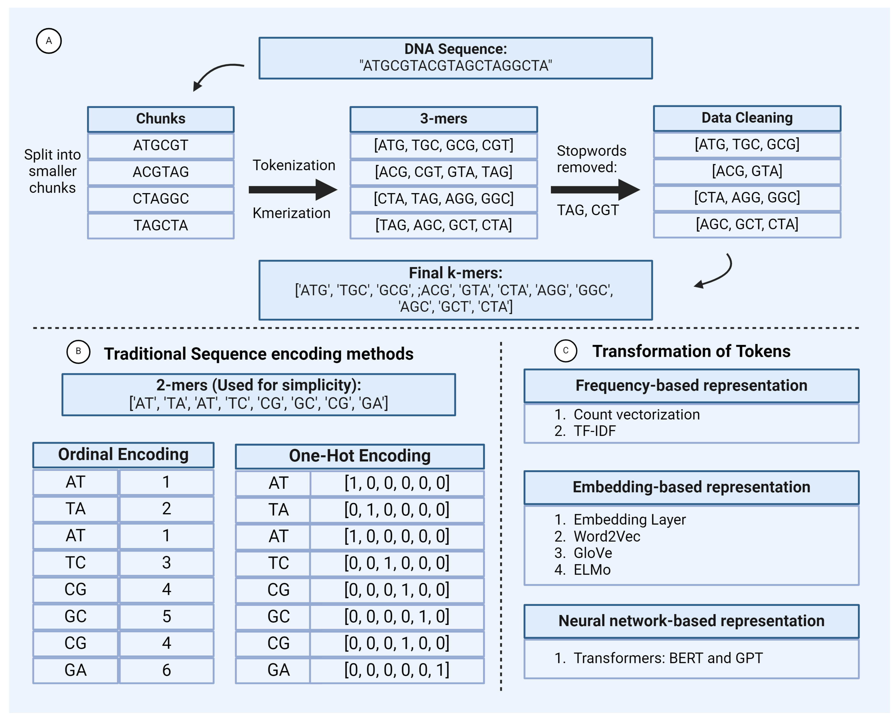
Figure 1. A GLM Workflow cheat sheet illustrating the following: A) The complete process of fragmenting long DNA sequences into smaller chunks, tokenizing them as 3-mers, and then performing stopword removal. B) Traditional methods for encoding or transforming DNA sequences, including ordinal and one-hot encoding. C) Advanced approaches to token transformation using frequency-based representation, embedding, and neural network representation.
Preprints 138447 g001
Figure 2. This figure illustrates examples of: A) Level of Tokenization: The section illustrates the various levels of tokenization applied to a DNA sequence input, producing different tokenized outputs. B) Types of Sub-word Tokenizers: The second section gives examples of four subword tokenization techniques: BPE (Byte-Pair Encoding), Unigram, WordPiece, and SentencePiece, showing how each method segments a DNA sequence into sub-word units.
Preprints 138447 g002
Figure 3. Transformation of DNA sequences using frequency-based representations: Count-vectorization and TF-IDF. The example illustrates how DNA sequences are tokenized and then converted into a numerical format.
Preprints 138447 g003
Figure 4. Illustration of Word2Vec model applied to k-mer sequences: (A) Training sample showcasing how Word2Vec processes a k-mer sequence using a window size of 2, traversing through the sequence to capture context-based relationships between neighboring k-mers. (B) A sample k-mer embedding plot: A graphical representation of the k-mer embeddings generated by the Word2Vec model. The X and Y axes indicate the relative distance between the k-mers, reflecting contextual similarities. Dense clusters suggest high similarity between k-mers, while loosely clustered or outlier k-mers suggest lower similarity or significant deviation from central groups.
Preprints 138447 g004
Disclaimer/Publisher’s Note: The statements, opinions and data contained in all publications are solely those of the individual author(s) and contributor(s) and not of MDPI and/or the editor(s). MDPI and/or the editor(s) disclaim responsibility for any injury to people or property resulting from any ideas, methods, instructions or products referred to in the content.
Copyright: This open access article is published under a Creative Commons CC BY 4.0 license, which permit the free download, distribution, and reuse, provided that the author and preprint are cited in any reuse.
Prerpints.org logo

Preprints.org is a free preprint server supported by MDPI in Basel, Switzerland.

Subscribe

© 2024 MDPI (Basel, Switzerland) unless otherwise stated