Submitted:
05 November 2024
Posted:
06 November 2024
You are already at the latest version
Abstract
When a star is born, a protoplanetary disk made of gas and dust surrounds the star. The 1 disk can show gaps opened by different astrophysical mechanisms. The gap has a wall emitting 2 radiation which contributes to the spectral energy distribution (SED) of the whole system (star, disk 3 and planet) in the IR band. As these new-born stars are far away from us, its difficult to know 4 whether the gap is opened by a forming planet. I have developed RHADaMAnTe, a computational 5 astro code based on the geometry of the wall gap coming from hydrodynamical 3D simulations of 6 protoplanetary disks. With this code it is possible to make models of disks to estimate synthetic SEDs 7 of the wall gap and prove whether the gap was opened by a forming planet. I have implemented this 8 code to the stellar system LkCa 15. I found that a planet of 10 Jupiter masses is capable of opening a 9 gap with a curved wall with height of 12.9AU. However, the synthetic SED does not fit to Spitzer IRS 10 SED (ξ2 ∼ 4.5) from 5µm to 35µm. This implies that there is an optically thick region inside the gap.
Keywords:
protoplanetary disk
; wall gap
; spectral energy distribution
; 3D simultaions
1. Introduction
In a small fraction of young stellar objects (YSOs) surrounded by disks, observations have discovered a low excess radiation in the near–infrared but a high excess in longer wavelengths. This has been interpreted as an evidence that these disks called transitional disks (TDs) have central holes which have practically no dust [1]. More recently, disks showing a significant excess in the near–infrared have been discovered. Such an excess indicates the presence of an optically thick inner disk. This inner disk is separated from an outer disk which also has a high optical depth. In this way the spectral energy distribution (SED) suggests the incipient development of a gap between both disks, these disks are called pre–transitional disks (Pre–TDs) [2]. Several physical mechanisms have been suggested to explain the gaps or holes in protoplanetary disks. The one implemented in this work is driven by forming giant planets.
A key element that produces characteristic features in the SEDs of protoplanetary disks is the outer wall of the gap or hole. To simplify SED wall models, it is often assumed that the wall is vertical and frontally irradiated by the central star [2,3]. But this assumption is physically wrong [4]. For dust sublimation walls, located near from the star, it has been proposed that the wall is curved, where the dust grain growth and its fall into the mid–plane of the disk, and the gas density high–dependence on sublimation temperature are the physical mechanisms responsible for such curvature [5].
In order to create synthetic SEDs of protoplanetary disks with gaps or holes having inner curved walls, I have developed a computational code called rhadamante. This code is based on an older code which suggests that the inner vertical wall of the outer disk can explain the mid–infrared spectrum of the low–mass pre main–sequence star CoKu Tau/4 [6].
To test the code, I present a model of a truncated dusty disk –a disk with an inner hole– that accounts for the Spitzer Infrared Spectrograph observations of the low-mass pre main–sequence star LkCa 15. In this model the mid–infrared spectral energy distribution (between 10 and 25µm) arises from the inner curved wall of the gap in the disk.
1.1. Dust in Protoplanetary Disks
Dust is a pretty important component of protoplanetary disks surrounding young stars. The growth of dust grains from sizes of microns to centimeters or larger grains is the first step in planet formation.
The dust grains in protoplanetary disks follow a size distribution based on a single power law [[7], MNR], where the maximum dust size, , the minimum dust size, , and the power law index, p, are different for each grain species.
The dust composition in protoplanetary disks has been extensively studied through mid-IR observations. This dusty mixture includes silicates (mainly), carbonaceous grains, poly-cyclic aromatic hydrocarbons, and sulfide-bearing grains [8].
Silicate grains are the best understood dust component. The most abundant crystalline silicates are olivine, which is magnesium-rich (Fo90), and pyroxene. Olivine series range from forsterite, Mg2SiO4 (denoted as Fo100), to the fayalite, Fe2SiO4 (denoted as Fo0). While pyroxene series range from the enstatite, MgSiO3 (denoted En100), to the ferrosilite, FeSiO3 (denoted En0).
Modeling of the observed spectra expects amorphous silicate grains to exist in protoplanetary disks [see, e.g. [9]; [10]]. The composition of these grains are glass with embedded metals and sulfides, and series ranging from ferromagnesian silica to Fe–Mg-bearing aluminosilica. These grains are difficult to observe directly from infrared spectroscopy. Their spectral signature observed is a combination of grain composition, shape, size, and structure, making difficult to isolate the pure amorphous silicate signal.
Carbonaceous grains, including amorphous and graphite elemental carbon, are difficult to detect in the infrared. However, grain modeling suggests these grains are needed in order to explain the observed infrared spectra of protoplanetary disks [9].
Nano–diamonds, from sizes of <1 nm to ∼ 10 nm, are found in protoplanetary disks. Diamond emission coming from the inner region of the disk (i.e. < 15 AU) at 3.43 and 3.53 m has been detected in disks [see, e.g. [11]].
The presence of poly-cyclic aromatic hydrocarbons (PAHs) has been detected in the surface layers of some protoplanetary disks [see, e.g. [12]]. Disks surrounding higher-mass stars, such as Herbig stars, show more PAHs emission [13] than disks surrounding lower-mass stars, such as T Tauri stars [14]. Protoplanetary disks with a flaring outer surface show significantly more PAH emission [13]. It follows that PAHs exist in all disks, but they can only be detected, as infrared emission, when ultraviolet radiation from the central star is able to excite them. The discovery of weak PAH features in T Tauri stars supports this idea [see, e.g. [14]].
Other dusty components in protoplanetary disks are iron-nickel sulfides grains (FeS, NiS) and water ice (H2O). Sulfide emision around 23 m has been detected in the emission spectra of protoplanetary disks [15]. While water ice emission has been identified at 3m [16], 44m [17], 60m [18] and 62m [19].
1.2. LkCa 15
LkCa 15 is a K5-type [20] T Tauri star located in the nearby () the Taurus-Auriga Star Forming Region [21]. The mass of the central star is [20], it has an effective temperature of 4370K [22] and a radius of [23]. Three planet candidates have been detected: LkCa 15b (semi major axis ) [24], LkCa 15c () and LkCa 15d (), with masses lower than 5–10, for the two first planets, and for the third one [25].
Observations of the far-ultraviolet (1100–2200Å) radiation field and the near–to mid–IR (3-13.5m) spectral energy distribution of LkCa 15, from the Space Telescope Imaging Spectrograph (STIS) indicate the existence of an inner disk gap of a few astronomical units [26].
LkCa 15 has an inner disk, a gap and an outer disk [27]. Using the Spitzer data, LkCa 15 has been classified as a pre-transitional disk [28], and it has been showed that the inner hole is not devoid of dust between 0.1 and 5 AU. The outer disk extends from 46 to 800 AU [29].
Recent observations from Gemini NIRI suggest that a single massive planet would be capable of opening a gap as large as the one observed in the LkCa 15 disk [22]. This assumption leads me to use a mass of ∼ for the planet candidate in the current work.
2. Geometry of the Wall Projected on the Sky
To find the two–dimensional geometry of a wall gap, I implement the artemise code [4]. Which is a computational and geometrical code that analyses a tri–dimensional simulation of the disk–planet interaction by considering the wall is located at the points where the disk optical depth is . Simulations are done with fargo-3D code [31] under some specific parameters of the young stellar object to be studied.
2.1. Inclined Walls
Definition 1.
In the coordinate system the star is centered at the origin, here z–axis is the disk rotation axis, and the plane is the disk mid–plane. For simplicity, I also consider the cylindrical coordinate system , such that all points on the wall superior boundary have coordinates z, y , whereas all points on the wall inferior boundary have coordinates z, y . Since the protoplanetary disk is assumed to be projected on the plane of the sky , as seen in Figure 2, I consider a third coordinate system also centered at the star, where the Z–axis is the line of sight. When the disk is face–on the coordinate systems coincide. There exists a transformation between the three coordinate systems:
where i is the disk inclination angle, that is, the angle between the z–axis and the plane of the sky .
The amount of visible surface of the wall, projected on the plane of the sky, depends on the disk inclination angle, and there are two possibilities: (i) when the star is visible (corresponding to , see Equations (4) and (9) for a definition of ), and (ii) when the star in invisible (corresponding to , as seen in Figure 2. A surface element of the visible area is , with .
Let be the visible surface of the wall projected on the plane for both cases, as seen in Figure 3. Then the boundary of this region is defined by two ellipses and (see Appendix A.1) given by the projections of the up and down edges of the tri–dimensional conic wall. The up ellipse is defined as , where and are the superior and inferior parts of this ellipse, respectively, such that
Similarly, the down ellipse is defined as , where and are the superior and inferior parts of this ellipse, respectively, such that
Ellipses and intersect at critical angles y , where is given by
Depending on the wall inclination angle i, there exist two possibilities to know whether both ellipses can intersect: if or not if , as seen in Figure 3.
For the case , the region is composed by two sub-regions and :
For the case , the region is defined as follows
2.2. Vertical Walls
If in Definition 1 I set , I obtain a two–dimensional vertical wall, as seen in Figure 4a. By rotating this line segment around z–axis, I generate a cylindrical ring which lies in the Euclidean space , as seen in Figure 4b. This ring is a tri–dimensional cylindrical wall.
Following the same mathematical procedure as in the case of an inclined wall, I obtain that
where
Both ellipses intersect at critical angles y , where is given by
3. The RHADaMAnTe Code
To create synthetic SEDs as arising from the inner curved wall of a gap or hole open by a planet in a protoplanetary disk, I have developed a computational code, written in the fortran 90 language, called rhadamante. This code is coupled to the artemise code because the geometry of the wall is required.
As I am interested in estimating the radiation reemitted by a tri–dimensional wall projected on the plane of the sky, in this code, I firstly calculate the angle between the radial ray and the normal to the two–dimensional wall for each incident radial radiation ray coming from the central star, as seen in Figure 5, by applying an algorithm also called RHADaMAnTe.
Then, I construct the tri–dimensional wall as the finite union of tri–dimensional conic rings obtained by rotating inclined line segments about the z–axis at different heights. (see Figure 6a and Figure 7).
Next, I calculate the surface projection on the plane of the sky of these rings, and then I calculate the radiation emitted by each of them by implementing some ideas from an algorithm developed for vertical walls [6]. Finally, I sum the contribution of the emission of all the projected rings to create a synthetic SED.
3.1. Geometry of the Radiation Reemitted by the Wall
rhadamante, acronym for Radial Geometry Algorithm for Calculating the Radiation Emitted by a Wall), it is a geometrical algorithm which at first calculates the angle between the stellar radiation along a radial ray and the normal to the two–dimensional wall , as seen in Figure 5. Secondly, this algorithm discretizes the two–dimensional wall, which is not continuous, as seen in Figure 6a.
Let be the angle between the normal on the point belonging to the wall , and the stellar radiation ray , such that
where is the minimal angle between the normal and the mid–plane (r–axis), and is the angle between the ray and the mid–plane, as seen in Figure 5.
The angle is required to calculate the reemitted stellar radiation by the wall. Because of wall’s curvature and the radial geometry of the stellar radiation, each parcel of the wall does not absorb the total radiation, as it is in the case of vertical walls. In this case, each parcel absorbs only a fraction of the radiation which depends on the .
Let be the tangent line to the wall at the point with a positive slope . It follows that the inclination angle of such a line, measured from the r–axis, is , where
Physically, the wall should be characterized by a mathematical continuous function. However, in this case, because of the numerical simulation, the wall is transfered, via the discretization process described in Section 3.2, into a discrete counterpart. So, as the points with defining are close enough, it is possible to find an approximation of its derivative.
Consider the points and in the wall to be connected along the segment line (as seen in Figure 5), then the slope of this line approximates to the derivative with respect to r of at the point , that is
Hence .
Next, since the line is almost perpendicular to the normal , it follows
Finally, since the star is located at the origin of coordinate system, it is easily to calculate the angle between the ray and the mid–plane
where and are the r and z coordinates of the point .
3.2. Discretization of the Two–Dimensional Wall
By applying the ARTeMiSE algorithm, I obtain a set of points with , defining the two–dimensional wall . It means that the wall is not a continuous curve. Then I discretize the wall as the finite union of infinitesimal inclined walls: I connect each couple of points and by inclined line segments with height , as seen in Figure 6.
Consider an inclined line segment with boundaries and in the wall , and let be the mid–point of . As I require that the vertical height of this line segment to be , I define
where and are the z coordinates of and the mid–point between the points and . See Figure 6.
If , I construct a vertical line segment with boundaries and , and height , which conects to the mid–plane.
3.3. Curved Wall
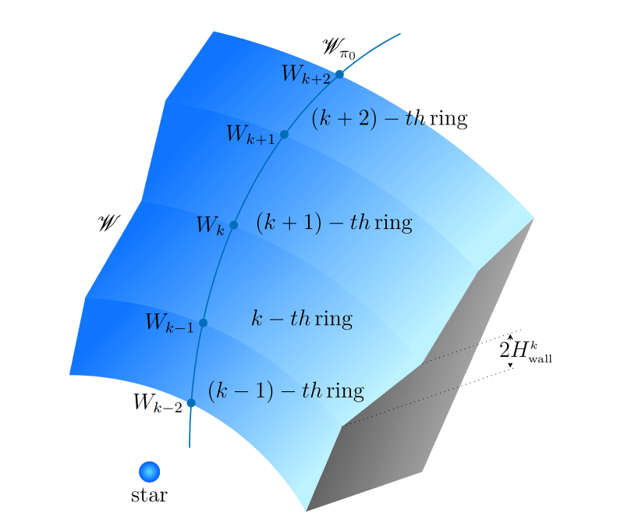
Let be a two–dimensional wall discretized by infinitesimal inclined line segments for , and a vertical line segment .
By rotating each inclined line segment around z–axis, one generates a conic ring with minimum radius , maximum radius and total height . Whereas, by rotating the vertical line segment, a cylindrical ring with radius and total height , is obtained. It follows the tri–dimensional curved wall can be defined as the finite union of a cylindrical ring and several conic rings: . See Figure 7.
3.3.1. Projection on the Plane of the Sky
The wall has to be projected on the plane of the sky to calculate the amount of visible surface. Therefore I consider the coordinate system , where Z is along the line of sight, such that
Since I want to apply the same algorithms of projection described in Section 2.1 and Section 2.2, it is required to do a geometric translation of each ring to a secondary coordinate system such that the translated ring is centered at the origin. Easily I can say that there exists a translation transformation :
where is the displacement of the ring along z–axis, to be centered at the origin of the system , see Figure 8, with is the z coordinate of the point and .
Applying this translation, it is possible to use the coordinate system to project the ring on the plane :
From Equations (13), (14), and (15) it follows that there exists a translation transformation , such that:
where is the projection on the Y–axis of the displacement of the ring along the z–axis, as seen in Figure 8.
Combining Equation (16) with Equations (2) and (3), it follows that for the k–th conic ring
Whereas, for the cylindrical ring, by combining Equation (16) with Equation (8), it follows
3.4. Emission of the Wall
To calculate the emission or emergent flux of the visible wall projected on the plane of the sky, I multiply the total emergent intensity by the solid angle of the visible surface of the wall, whose geometry has been described in detail in Section 3.3.
For each element in the visible surface of the projected wall, the thermal emergent intensity, approximated as isotropic, is given by
[see [6] for derivation], where is the Planck function, is the total mean optical depth at the disk frequency band, and , with opacity .
The wall temperature is a function of the optical depth of the disk, and it is calculated as follows [see [6] for derivation]
where
and
with , , and is the mean albedo to the stellar radiation and , where is the stellar luminosity.
At a distance d from the observer, the total solid angle is given by
with
for conic rings, and
with
for cylindrical rings.
3.4.1. Rosseland Mean Opacity
Equation (19) requires the calculation of the opacity . This dominant opacity depends on the chemical composition, pressure and temperature of the gas, as well as the frequency of the incident light. This is a complex endeavour. The problem can be simplified by using a mean opacity averaged over all frequencies, so that only the dependence on the gas physical properties remains. In the current work, I use the Rosseland mean opacity, defined as
where is the Planck’s function, and T is the disk temperature [32].
To calculate the total Rosseland mean opacity , I consider that all the dust grains species exist and the mixture of dust grains is made of small and big grains. Using the previous assumptions I calculate the total Rosseland mean opacity as follows:
where and are the Rosseland mean opacities associated to the small dust grain size distribution and big dust grain size distribution, respectively. And and represent the abundances (dust-to-gas mass ratio) of the small and big grains, respectively:
here represents a small fraction of the scale height of the disk, and k is a factor which defines a smooth transition between small and big grains population [33].
The monochromatic opacity in Equation (25) depends on the dust species in the mixture and their physical and chemical properties, such that it is calculated as the sum of the monochromatic opacity of each grain species:
where and are the sizes of the small and big grains, and and are the abundance and refraction index of the species. Here q is running over the name of the species (e.g. silicates, organics, amorphous carbon, ice and troilite) in the dust composition of the disk. I calculate the monochromatic opacities using the Mie theory by implementing some modified routines of a code developed in [6].
Summarizing, to calculate the emergent flux emitted by the curved wall, I have developed a computational code called rhadamante. This code is based on the geometry of the wall calculated by the artemise code. In Figure 9 I show a flowchart of our code. For some tests, see Appendix B.
4. Results: An Implementation to the Stellar System LkCa 15
In this section, I present a model of the truncated dusty disk of the T Tauri star LkCa 15 that accounts for the Spitzer Infrared Spectrograph observations. I have modeled the mid–infrared spectral energy distribution from 5 and 40) as arising from the inner curved wall of the outer disk. In this model a mass planet is the responsible of the wall curvature. The free dust hole has a radius of ∼ along the mid-plane. The wall has a half-height of ∼ and it is illuminated at normal incidence by the central star, but it also is shadowed because of the presence of an internal optically thick disk.
4.1. Simulation: Planet–Disk Interaction
As I am interested in characterizing the geometry of the wall of the disk gap, in the LkCa 15 system, I need to analyze the vertical structure of the disk. Assuming the gap was opened by an embedded planet, I use the fargo–3d hydro–dynamical code to launch two numerical simulations of the disk–planet interaction until the 500th. The only difference among these simulations is the size in resolution (). The low resolution of was used to find quickly the orbit where the system reaches a quasi–stationary state. The medium resolution of was used to get a better approximation of the wall. According to fargo–3d requirements, in Table 1 I show some parameters for simulations.
In Figure 10, I present the tri–dimensional structure of the 100th orbit of the LkCa 15 disk simulation. It is here where the system reached a stationary-state.
4.2. Dust Grain
The optical depth of the disk depends on the disk material opacity, I assume that the disk is a mixture of grains composed of silicates with mass fraction , organics with , and troilite with , consistent with the model proposed in [34]. The grains are assumed to be spheres, which obey the standard MRN grain size distribution [7].
I consider two grain populations: small grains between minimum radius and maximum radius , and big grains between minimum radius and maximum radius . I consider a smooth transition between both dust populations, see Equation (27) in Section 3.4.1, where I set , and and . I use optical constants for silicates from [35,36] and [37], for the organics from [34] and for troilite from [34] and [38]. I also take into account the sublimation temperature of the grain species in the mixture , , and .
4.3. The Vertical Geometry of the Wall
I found that the mass planet candidate, when is located at from the central star, opens a gap around the young transitional disk host LkCa 15. The artemise code was implemented to analize the simulation data. The radii of the wall along the mid–plane of the disk and the heights of the wall have a deppendence on the chemical composition of the silicate grains as showed in Table 2. In Figure 12, I show the geometry of a wall where the dust garin disk composition has glassy olivine (silicate) with 50%Fe and 50% Mg.
The location of the planet candidate is not consistent with the observations [e.g. [25], which suggest that the possible massive planets LkCa 15 b and LkCa 15c are located at and , respectively, along the semimajor axis. However, the radii of the wall along the mid–plane are similar to those measured in [40,41], ∼, and [22],∼.
4.4. SED of the Wall
I model LkCa 15 as a central star with the properties described in Section 1.2, surrounded by an optically thick inner disk (as showed in Figure 11) and and outer disk truncated at ∼. I consider the gap has a curved wall at differentent locations and heights according to Table 2. In the models, I consider that LkCa 15 is at from Earth in the Taurus-Auriga star forming region [21] and the disk inclination is [25]. A representation of the model is showed in Figure 13.
As the inner disk casts an umbra over the wall of the outer disk, as seen in Figure 13, I have to remove it from the SED of the outer disk wall. In order to find , I implement some improved routines developed in [42] for curved sublimation walls. This code uses opacities to calculate the shape of the wall and assumes that the stellar rays are parallel to the mid–plane. I found that the wall of the inner disk starts at ∼, from the central star, and runs until ∼ where it reaches ∼ in height. And the temperature of the sublimation wall decreases with radius and it ranges from to .
In a first approximation, assuming the star as a point, the sublimation wall produces only an umbra over the wall of the outer disk (see Figure 13). To calculate the size of this umbra, theangle subtended by the height of the sublimation wall is needed. In addition, for some points in the outer wall, I calculate the angle until it reaches the value .
Applying the previous algorithm to the geometry of the wall (see Figure 12), I found that the umbra produced by the sublimation wall of the inner disk onto the wall of the outer disk is in height (above and below the disk mid–plane). It means the contribution to the SED of the outer wall comes from a region of the wall from ∼ to ∼ along the radial direction, and from to along the vertical direction. In Figure 14a I show the surface area of the whole curved wall, and in Figure 14b I show the surface area considered the umbra cast by the inner disk.
Synthetic SEDs of the wall of the outer disk, where the dust consists of grains of glassy pyroxene with different concentration of Fe and Mg are showed in Figure 15. I performed a chi–square test for each model, to examine whether the synthetic SED fits to the Spitzer IRS SED. I found that no model is either capable to fit the observed SED (∼300) nor reproduce the silicate peak at ∼. However, for glassy pyroxene with 60% Fe and 40% Mg (see Figure 15a) it seems the silicate peaks tries to appear at ∼, this lead us to think that a lesser concentration of Mg in the pyroxene composition would produce the silicate feature. Unfortunately, there is not available, in the literature, the optical constants needed to calculate the opacities, for such chemical concentrations.
In Figure 16, I show the synthetic SEDs of the wall of the outer disk, where the dust mixture consists of grains of glassy olivine with different concentration of Fe and Mg. I found that none of these configurations is capable to fit the observed SED (). However, in both cases a silicate peak appears at ∼. A concentration of 50% Fe and 50% Mg produces the best fit (see Figure 16b).
Previous results lead us to say that the SED of LkCa 15 is not dominated by the contribution of the curved wall of the outer disk in the mid–infrared. However, when olivine grains with a concentration of 50% Fe and 50% Mg or 80% Fe and 20% Mg are in the dust mixture, a silicate feature appears at ∼.
4.5. SED of the System
Considering the SED contribution of the inner sublimation wall and the star, in addition to the SED contribution of the wall of the outer disk, I present a more complete model of the stellar system LkCa 15. For the stellar SED, I have used a Kurucz atmosphere model with and . Table 3 lists the parameters for this model. In Figure 17, I show the contribution of the star, the inner sublimation wall and the wall of the outer disk to the total synthetic SED.
Only for some wavelengths in the mid–infrared, ∼∼, the sythetic SED fit to LkCa 15 observed SED, I estimated ∼. For all the other wavelengths in the field of view of the Spitzer IRS (5.217–37.86 m), the synthetic SED is below the observed SED. For wavelengths ∼∼ the difference is not very high (∼); however, for wavelengths ∼∼ (with ∼) and ∼∼ (with ∼) this difference becomes significant (see Figure 18).
I can suggests that the inner sublimation wall and the stellar photo-sphere cannot account for the significant near-infrared excess in LkCa 15. It means the SED model also requires of optically thin dust inside the gap to explain the excess and to produce the silicate feature as showed in [43]. Similarly, as the wall of the outer disk cannot account for the excess in the mid and long–infrared, I asumme that this SED model also requires of the contribution of the outer disk.
5. Discussion: Vertical Wall SED vs. Curved Wall SED
Wall SED models of LkCa 15 (and many other pre-TDs and TDs) are based on vertical walls [e.g. [23,43]]. rhadamante code is able to construct wall SEDs based on this geometry. Here I present some wall SED models of LkCa 15 considering vertical walls to compare with the best fit curved wall SED model (as seen in Figure 19).
In these vertical wall SED models, it is also cosidered that the umbra cast by the inner disk is (measured from the disk mid–plane to up). The height of the wall is (measured from the disk mid–plane to up). The size and composition of the dust grains remain the same as described for the best fit curved wall SED model.
The vertical walls were located at 30, , and . rhadamante estimated the area of the visible surface projected on the plane of the sky of these vertical walls, , and the curved wall, . I found that , if the umbra of the inner disk is considered. While if the emission of the whole wall is considered, . Wall temperatures also were estimated, I found , , and , respectively. It means that the temperature of a vertical wall, , decreases if its radius, , increases. Furthermore, the radiation emitted by a vertical wall, , also decreases as increases, as seen in Figure 19.
Finaly, I compared the radiation emitted by vertical walls, , with the radiation emitted by the curved wall, (see Figure 19). I found that for wavelengths between 5 and . The difference between fluxes becomes significant, about one order of magnitude, for .
This infrared excess arises, in part, from the angle, , between the radiation ray and the normal to the wall (see Section 3.1), because . For vertical walls, for all the radiation rays hitting the wall, because the normal to the wall is always parallel to the disk mid–plane. Whereas for curved walls , because of the wall curvature. In addition, for some models, some regions of the curved wall are farther from the central star than the vertical one.
The above two facts induce a lower exposure of the curved wall to the host star radiation, which derives in much less radiative heating of the wall, and, consequently, in the significantly lower radiative infrared cooling flux. For this reason, the one order of magnitude in lower infrared emisison in the curved wall model is as significant as correct by very basic physical considerations: the height of the curved wall and the umbra cast by the inner disk onto the outer disk.
It is worth mentioning that the geometry, location and height of the curved wall arise from a physical mechanism considering the opacities and chemical composition of the disk, where the disk is the result of a three–dimensional hydro–dynamical simulation, whereas for the vertical walls there is not any physics to choice these parameters. Although the curved wall SED model is the best choice to compare with the Spitzer IRS SED of LkCa 15, as it is showed in Figure 19, to rise this synthetic flux to the right level, it is needed, in adittion, the contribution of the central star, the inner disk, the outer disk and a region of optically thin dust inside the gap, as discussed in Section 4.4.
6. Conclusions
The computational code rhadamante was developed in order to calculate synthetic SEDs of protoplanetry disks. As a initial parameter, the code requires the geometry of the wall coming from hydro-dynamical three-dimensional simulations of the planet-disk interaction and dust grain properties. This code is useful to explain the observed SED of young stellar systems in transition stage. It would lead to unveil the structure of the system, such as, the inner disk, the gap, and the outer disk, even the location and mass of the embedded planet responsible of the gap opening.
From the implementation of this code to the pre-transitional disk LkCa 15, it can be concluded that:
All models of the SED consisting only of a curved wall, using different concentrations of Fe and Mg for the silicate (pyroxene and olivine) grains, suggest that LkCa 15’s Spitzer IRS SED cannot be accounted by the emission of a curved wall. Chi-square tests indicate the models are not good (∼). In addition, for models with a dust mixture containing glassy amorphous olivine grains, or , a silicate feature can be observed. However, the intensity of this silicate emission to that measured in the Spitzer IRS SED.
Including to the wall SED model, the contribution of the stellar photo-sphere and the sublimation wall of the inner disk, considering a dust mixture with amorphous glassy olivine with 50% Fe and 50% Mg and a small amount of organic and troilite grains, the observed and synthetic SEDs fit better (∼45). However, this model cannot fit the Spitzer IRS SED. Only for a small band in the mid-infrared, ∼∼, the fit is good (∼).
Several limitations exist in the current model: The contribution of the inner disk was not considered, neither the contribution of an optically thin region inside the gap [e.g. [23,43], nor the optically thick outer disk. The inner disk might contribute to the SED at wavelengths in the near infrared. The optically thin region might explain the silicate feature of the Spitzer IRS SED at . While the outer disk might contribute to the SED at wavelengths longer than .
Vertical wall SED models, via rhadamante code, show a difference of one order of magnitude in the flux, , compared to the curved wall SED model, , for wavelengths from 8 to . This difference arises from dependency of the flux, , on the cosine of the angle, , between the stellar radiation ray and the normal to the wall. This lower exposure of the curved wall to the stellar radiation results in much less radiative heating of the wall, and, consequently, in the significantly lower radiative infrared cooling flux.
The synthetic SED of a curved wall, estimated by rhadamante code, includes physical and chemical mechanisms absent in the estimation of the SED of a vertical wall. That is, a curved wall SED is better to fit the Spitzer IRS SED of LkCa 15 or any other protoplanetaray disk.
Funding
“This research was funded by Consejo Nacional de Humanidades, Ciencia y Tecnología (CONAHCyT) grant number CF-2023-I-1221.”
Conflicts of Interest
“The author declares no conflicts of interest.”
Abbreviations
The following abbreviations are used in this manuscript:
| Mass of the Sun | |
| Mass of Jupiter |
Appendix A. Mathematical Tools
Appendix A.1. Construction of a Vertical Wall
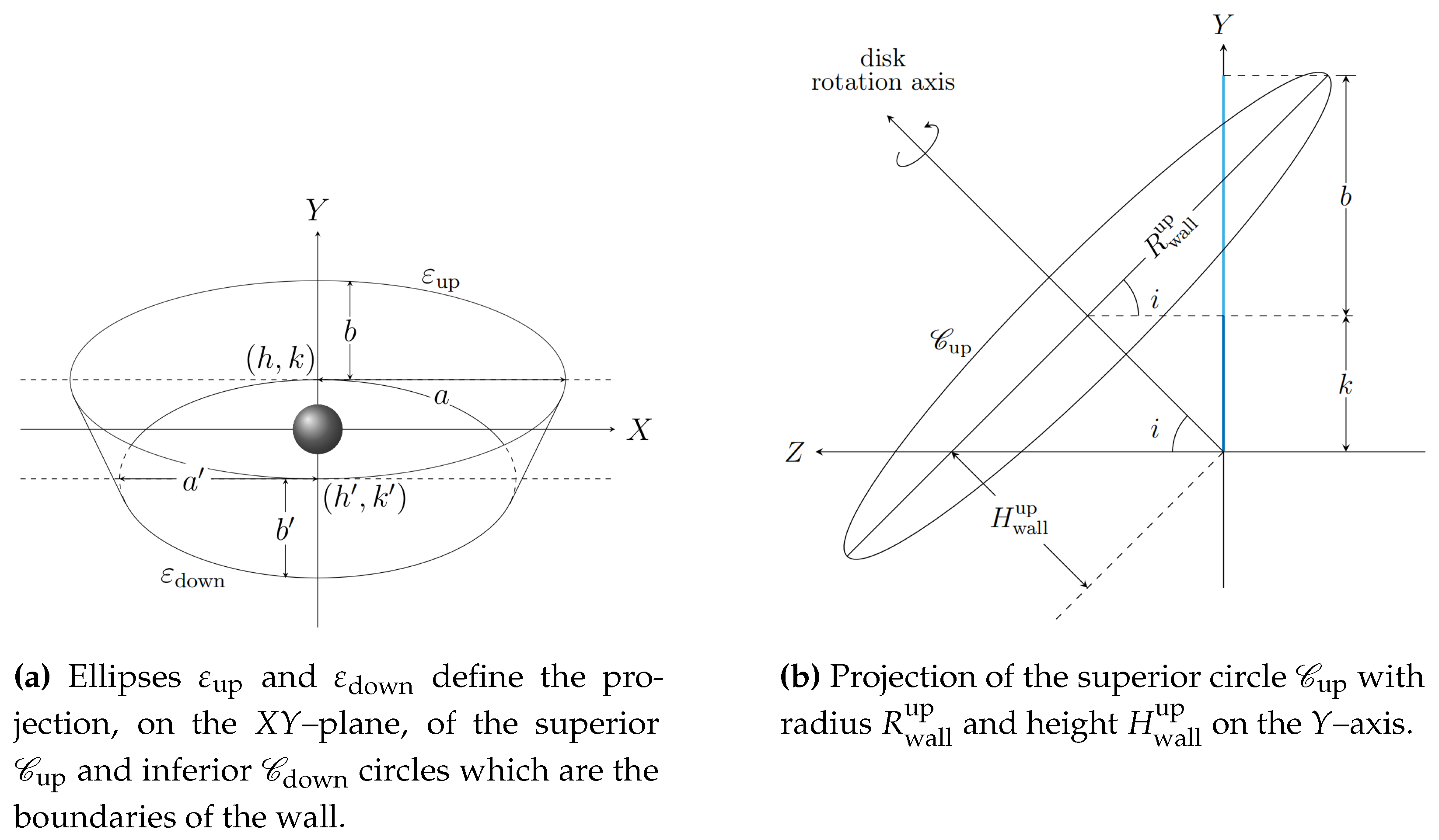
Consider an inclined segment line as showed in Figure 1a. Circles and , with radii and and height and , respectively, are generated by rotating such segment line around z–axis. These circles define the superior and inferior boundaries of a tri–dimensional wall . The projection on the –plane of these circles, given an inclination angle i, generates the ellipses and , as seen in Figure A1a. Ellipse is centered at with semi–major and semi–minor axes a and b, respectively. Whereas, ellipse is centered at with semi–major and semi–minor axes and , respectively.
Without lost of generality I focus on the construction of ellipse . As the coordinate system is centered on the star, it follows , and the Y coordinate of the ellipse is the projection of the height of the circle on the Y-axis, as seen in Figure A1b, that is, . The semi–major axis is , and the semi–minor axis is the projection of the radius of the circle on the Y-axis, as seen in Figure A1b, that is, .
Figure A1.
Geometry of ellipses and defining the projection of the tri–dimensional wall on the –plane.
Figure A1.
Geometry of ellipses and defining the projection of the tri–dimensional wall on the –plane.
So the full form of the equation of ellipse is:
Similarly, for ellipse ,
Hence, I define
such that
Appendix A.2. Area Between Two Curves
Definition A1.
The area between the curves and and the ordinates and is given by
if and only if .
Definition A2.
Let be a continuous function defined by . An anti-derivative or primitive function of f is
such that .
Appendix A.3. Theoretical area of the projected vertical wall: The whole wall
The following analysis, on the area of a visible wall (projected on the plane of the sky), focuses on the case corresponding to (the star is visible), because of LkCa 15 inclination angle ().
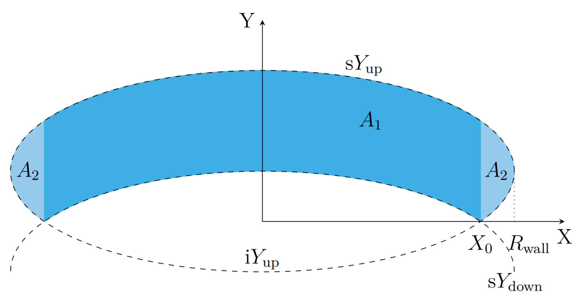
The area of the projection of a whole vertical wall on the plane of the sky is
as seen in Figure (Figure A2). Where, according to Definition A1,
and
Figure A2.
Area of the projection of the whole vertical wall on the plane of the sky , defined by the intersection of the ellipses and .
Figure A2.
Area of the projection of the whole vertical wall on the plane of the sky , defined by the intersection of the ellipses and .
Since
and
it follows
and
Using Equation (A6), it leads
Hence, the area of the projected vertical wall is
Appendix A.4. Theoretical Area of the Projected Vertical Wall: The Wall with Shadow
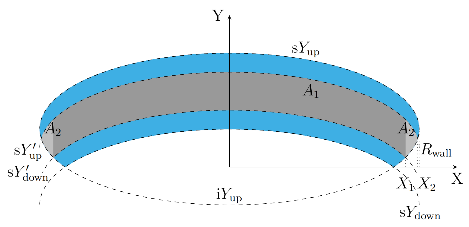
To calculate the area of the projection of a vertical wall considering the umbra cast by the inner disk, I subtract to the area generated by the whole wall [see Equation (A11)], the area generated by the shadow. The shadow can be assumed as a vertical wall with in height, measured from the mid–plane.
Then the area of the projection of the shadow on the plane of the sky is
as seen in Figure A3. Where, according to Definition A1,
and
with
Since
if follows
and
Figure A3.
Area of the projection of the shadow cast by the inner disk on the plane of the sky , defined by the intersection of the ellipses , and (in gray). The region in blue is the area of the visible wall.
Figure A3.
Area of the projection of the shadow cast by the inner disk on the plane of the sky , defined by the intersection of the ellipses , and (in gray). The region in blue is the area of the visible wall.
Using Equation (A6), it leads
Hence, the area of the shadow, projected on the plane of the sky, is
Appendix B. Testing RHADaMAnTe
rhadamante code calculates the Spectral Energy Distribution (SED) of the curved wall of gaps in protoplanetary disk. Before doing its main task, this code has to calculate the projection of each ring on the plane of the sky, which defines the 3D-wall. Figure A4 shows the results of a test where it is assumed that the 3D-wall is made of six rings.
Figure A4.
Wall surface projected on the plane of the sky calculated by rhadamnte.
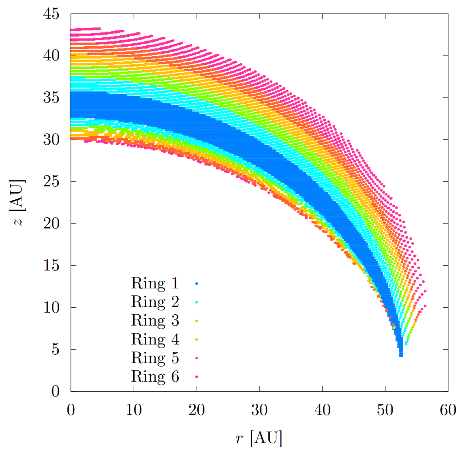
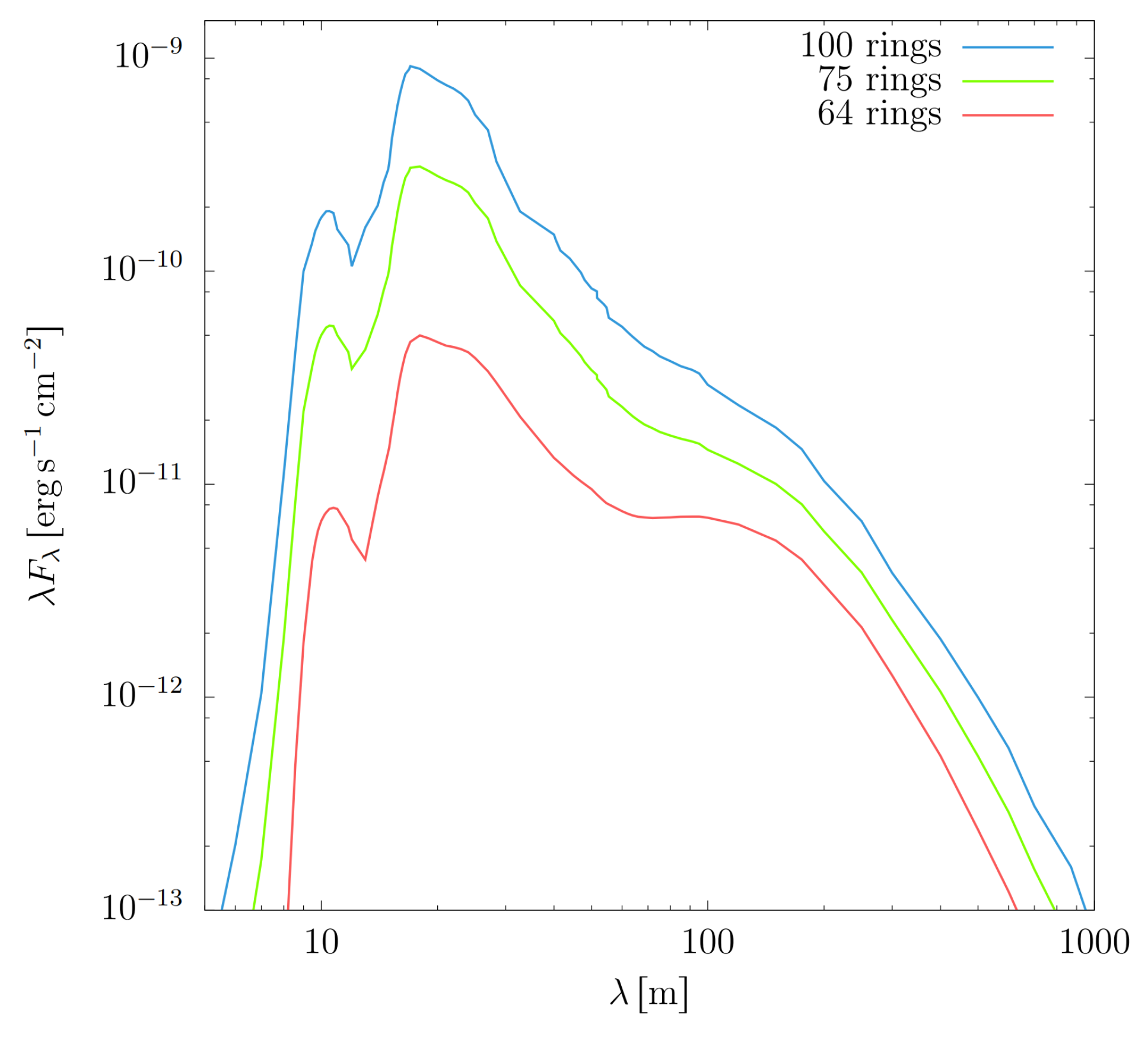
Figure A5 shows the synthetic SED of a curved wall depending on the number of rings used to estimate it. That is, as the number of the rings increases the size of the SED also increases. In the test it was noticed that the greater contributors to the SED are those rings near the mid-plane.
Figure A5.
SEDs of a curved wall with different ring contributions calculated by rhadamante. SED in blue is calculated using all the rings, that is, the whole wall. SED in green is calculated starting from the 14th ring above the disk-mid plane, and SED in red is calculated starting from the 36th ring, that is, a shadowed wall.
References
- Calvet, N.; D’Alessio, P.; Hartmann, L.; Wilner, D.; Walsh, A.; Sitko, M. Evidence for a Developing Gap in a 10 Myr Old Protoplanetary Disk. ApJ 2002, 568, 1008–1016. [Google Scholar] [CrossRef]
- Espaillat, C.; Calvet, N.; D’Alessio, P.; Hernández, J.; Qi, C.; Hartmann, L.; Furlan, E.; Watson, D.M. On the Diversity of the Taurus Transitional Disks: UX Tauri A and LkCa 15. ApJ 2007, 670, L135–L138. [Google Scholar] [CrossRef]
- Espaillat, C.; Calvet, N.; D’Alessio, P.; Bergin, E.; Hartmann, L.; Watson, D.; Furlan, E.; Najita, J.; Forrest, W.; McClure, M.; Sargent, B.; Bohac, C.; Harrold, S.T. Probing the Dust and Gas in the Transitional Disk of CS Cha with Spitzer. ApJ 2007, 664, L111–L114. [Google Scholar] [CrossRef]
- Rendón, F. Modelación de la geometría de paredes de cavidades en discos protoplanetarios mediante el código ARTeMiSE. In Modelación matemática V: Ingeniería, Ciencias Naturales y Ciencias Sociales; Reyes-Mora, S., Barragán-Mendoza, F., Eds.; Universidad Tecnológica de la Mixteca: Huajuapan de León, Oaxaca, México, 2023; pp. 57–75. [Google Scholar]
- Muzerolle, J.; Calvet, N.; Hartmann, L.; D’Alessio. Unveiling the Inner Disk Structure of T Tauri Stars. ApJ 2003, 597, L149–L152. [Google Scholar] [CrossRef]
- D’Alessio, P.; Hartmann, L.; Calvet, N.; Franco-Hernández, R.; Forrest W., J.; Sargent, B.; Furlan, E.; Uchida, K.; Green, J.D.; Watson, D.M.; Chen, C.H.; Kemper, F.; Sloan, G.C.; Najita, J. The Truncated Disk of CoKu Tau/4. ApJ 2005, 621, 461–472. [Google Scholar] [CrossRef]
- Mathis, J.S.; Rumpl, W.; Nordsieck, K.H. The size distribution of interstellar grains. ApJ 1997, 217, 425–433. [Google Scholar] [CrossRef]
- Min, M.; Flynn, G. Dust Composition in Protoplanetary Disks. In Protoplanetary Dust: Astrophysical and Cosmochemical Perspectives; Apai, D. A.; Lauretta, D.S., Eds.; Cambridge University Press, 2010; pp. 161–190.
- Min, M.; Hovenier, J.W.; de Koter, A.; Waters, L.B.F.M.; Dominik, C. The composition and size distribution of the dust in the coma of Comet Hale Bopp. Icarus 2005, 179, 158–173. [Google Scholar] [CrossRef]
- Lisse, C.M.; VanCleve, J.; Adams, A.C.; A’Hearn, M.F.; Fernández, Y.R.; Farnham, T.L.; Armus, L.; Grillmair, C.J.; Ingalls, J.; Belton, M.J.S.; Groussin, O.; McFadden, L.A.; Meech, K.J.; Schultz, P.H.; Clark, B.C.; Feaga, L.M.; Sunshine, J.M. Spitzer Spectral Observations of the Deep Impact Ejecta. Science 2006, 313, 635–640. [Google Scholar] [CrossRef]
- Habart, E.; Testi, L.; Natta, A.; Carbillet, M. Diamonds in HD 97048: A Closer Look. ApJ 2004, 614, L129–L132. [Google Scholar] [CrossRef]
- Meeus, G. , Waters, L.B.F.M.; Bouwman, J.; van den Ancker, M. E.; Waelkens, C.; Malfait, K. ISO spectroscopy of circumstellar dust in 14 Herbig Ae/Be systems: Towards an understanding of dust processing. A&A 2001, 364, 476–490. [Google Scholar]
- Acke, B.; van den Ancker, M.E. ISO spectroscopy of disks around Herbig Ae/Be stars. A&A 2004, 426, 151–170. [Google Scholar]
- Geers, V.C.; Augereau, J.-C.; Pontoppidan, K.M.; Dullemond, C.P.; Visser, R.; Kessler-Silacci, J.E.; Evans, N.J., II; van Dishoeck, E.F.; Blake, G.A.; Boogert, A.C.A.; Brown, J.M.; Lahuis, F.; Merín, B. C2D Spitzer-IRS spectra of disks around T Tauri stars. II. PAH emission features. A&A 2004, 459, 545–556. [Google Scholar]
- Keller, L.P.; Messenger, S.; Flynn, G.J.; Jacobsen, C.; Wirick, S. Chemical and Petrographic Studies of Molecular Cloud Materials Preserved in Interplanetary Dust. MaPS 2000, 35, A86. [Google Scholar]
- Terada, H.; Tokunaga, A.T.; Kobayashi, N.; Takato, N.; Hayano, Y.; Takami, H. Detection of Water Ice in Edge-on Protoplanetary Disks: HK Tauri B and HV Tauri C. ApJ 2007, 667, 303–3007. [Google Scholar] [CrossRef]
- van den Ancker, M.E.; Bouwman, J.; Wesselius, P.R.; Waters, L.B.F.M.; Dougherty, S.M.; van Dishoeck, E.F. ISO spectroscopy of circumstellar dust in the Herbig Ae systems AB Aur and HD 163296. A&A 2000, 357, 325–329. [Google Scholar]
- Malfait, K.; Waelkens, C.; Bouwman, J.; de Koter, A.; Waters, L.B.F.M. The ISO spectrum of the young star HD 142527. A&A 1999, 345, 181–186. [Google Scholar]
- McClure, M.K.; Manoj, P.; Calvet, N.; Adame, L.; Espaillat, C.; Watson, D.M.; Sargent, B.; Forrest, W.J.; D’Alessio, P. Probing Dynamical Processes in the Planet-forming Region with Dust Mineralogy. ApJ 2012, 759, L10–L16. [Google Scholar] [CrossRef]
- Simon, M. and Dutrey, A.;Guilloteau, S. Dynamical Masses of T Tauri Stars and Calibration of Pre-Main-Sequence Evolution. ApJ 2000, 545, 1034–1043. [Google Scholar] [CrossRef]
- Kenyon, S.J.; Hartmann, L. Pre-Main-Sequence Evolution in the Taurus-Auriga Molecular Cloud. ApJS 1995, 101, 117–171. [Google Scholar] [CrossRef]
- Thalmann, C.; Mulders, G.D.; Hodapp, K.; Janson, M.; Grady, C.A.; Min, M.; de Juan Ovelar, M.; Carson, J.; Brandt, T.; Bonnefoy, M.; McElwain, M.W.; Leisenring, J.; Dominik, C.; Henning, T.; Tamura, M. The architecture of the LkCa 15 transitional disk revealed by high-contrast imaging. A&A 2014, 556, A51–A74. [Google Scholar]
- Espaillat, C. and D’Alessio, P. and Hernández, J.; Nagel, E.; Luhman, K.L.; Watson, D.M.; Calvet, N.; Muzerolle, J.; McClure, M. Unveiling the Structure of Pre-transitional Disks. ApJ 2010, 717, 441–457. [Google Scholar] [CrossRef]
- Kraus, A. L.; Ireland, M.J. LkCa 15: A Young Exoplanet Caught at Formation? ApJ 2012, 745, 5–17. [Google Scholar] [CrossRef]
- Sallum, S.; Follette, K.B.; Eisner, J.A.; Close, L.M.; Hinz, P.; Kratter, K.; Males, J.; Skemer, A.; Macintosh, B.; Tuthill, P.; Bailey, V.; Defrère, D.; Morzinski, K.; Rodigas, T.; Spalding, E.; Vaz, A.; Weinberger, A.J. Accreting protoplanets in the LkCa 15 transition disk. Nature 2015, 527, 342–344. [Google Scholar] [CrossRef] [PubMed]
- Bergin, E.; Calvet, N.; Sitko, M.L.; Abgrall, H.; D’Alessio, P.; Herczeg, G.J.; Roueff, E.; Qi, C.; Lynch, D. K.; Russell, R.W.; Brafford, S.M.; Perry, R.B. A New Probe of the Planet-forming Region in T Tauri Disks. ApJ 2004, 614, L133–L136. [Google Scholar] [CrossRef]
- Najita, J.R.; Strom, S.E.; Muzerolle, J. Demographics of transition objects. MNRAS 2007, 378, 369–378. [Google Scholar] [CrossRef]
- Espaillat, C.; Calvet, N.; Luhman, K.L.; Muzerolle, J.; D’Alessio, P. Confirmation of a Gapped Primordial Disk around LkCa 15. APJ 2008, 682, L125–L128. [Google Scholar] [CrossRef]
- Piétu, V.; Dutrey, A.; Guilloteau, S.; Chapillon, E.; Pety, J. Resolving the inner dust disks surrounding LkCa 15 and MWC 480 at mm wavelengths. A&A 2006, 378, L43–L47. [Google Scholar]
- Andrews, S. M.; Williams, J.P. High-Resolution Submillimeter Constraints on Circumstellar Disk Structure. APJ 2005, 659, 705–728. [Google Scholar] [CrossRef]
- Benítez-Llambay, P.; Masset, F. S. FARGO3D: A New GPU-oriented MHD Code. ApJ 2016, 223, 29. [Google Scholar] [CrossRef]
- Hui-Bon-Hoa, A. Stellar models with self-consistent Rosseland opacities - Consequences for stellar structure and evolution. A&A 2021, 646, L6–L10. [Google Scholar]
- D’Alessio, P.; Calvet, N.; Hartmann, L.; Franco-Hernández, R.; Servín, H. Effects of Dust Growth and Settling in T Tauri Disks. ApJ 2006, 638, 314–335. [Google Scholar] [CrossRef]
- Pollack, J.B.; Hollenbach, D.; Beckwith, S.; Simonelli, D. P.; Roush, T.; Fong, W. Composition and radiative properties of grains in molecular clouds and accretion disks. ApJ 1994, 421, 615–639. [Google Scholar] [CrossRef]
- Jaeger, C.; Mutschke, H.; Begemann, B.; Dorschner, J.; Henning, T. Steps toward interstellar silicate mineralogy. 1: Laboratory results of a silicate glass of mean cosmic composition. A&A 1994, 292, 641–655. [Google Scholar]
- Dorschner, J.; Begemann, B.; Henning, T.; Jaeger, C.; Mutschke, H. Steps toward interstellar silicate mineralogy. II. Study of Mg-Fe-silicate glasses of variable composition. A&A 1995, 300, 503–520. [Google Scholar]
- Draine, B.T. Interstellar Dust Grains. ARA&A 2003, 41, 241–289. [Google Scholar]
- Begemann, B.; Dorschner, J.; Henning, T.; Mutschke, H.; Thamm, E. A laboratory approach to the interstellar sulfide dust problem. ApJ 1994, 423, L71–L74. [Google Scholar] [CrossRef]
- Henning, T.; Il’In, V.B.; Krivova, N.A.; Michel, B.; Voshchinnikov, N. V. WWW database of optical constants for astronomy. A&AS 1999, 136, 405–406. [Google Scholar]
- Piétu, V.; Dutrey, A.; Guilloteau, S. Probing the structure of protoplanetary disks: a comparative study of DM Tau, LkCa 15, and MWC 480. A&A 2007, 467, 163–178. [Google Scholar]
- Andrews, S.M.; Rosenfeld, K.A.; Wilner, D.J.; Bremer, M. A Closer Look at the LkCa 15 Protoplanetary Disk. ApJ 2011, 745, L5–L10. [Google Scholar] [CrossRef]
- Nagel, E.; D’Alessio, P.; Calvet, N.; Espaillat, C.; Trinidad, M. A. The Effect of Sublimation Temperature Dependencies on Disk Walls Around T Tauri Stars. RMXAA 2013, 49, 43–52. [Google Scholar]
- Espaillat, C.; Calvet, N.; D’Alessio, P.; Hernández, J.; Qi, C.; Hartmann, L.; Furlan, E.; Watson, D.M. On the Diversity of the Taurus Transitional Disks: UX Tauri A and LkCa 15. ApJ 2007, 670, L135–L138. [Google Scholar] [CrossRef]
Figure 1.
Construction of a tri-dimensional conic wall.
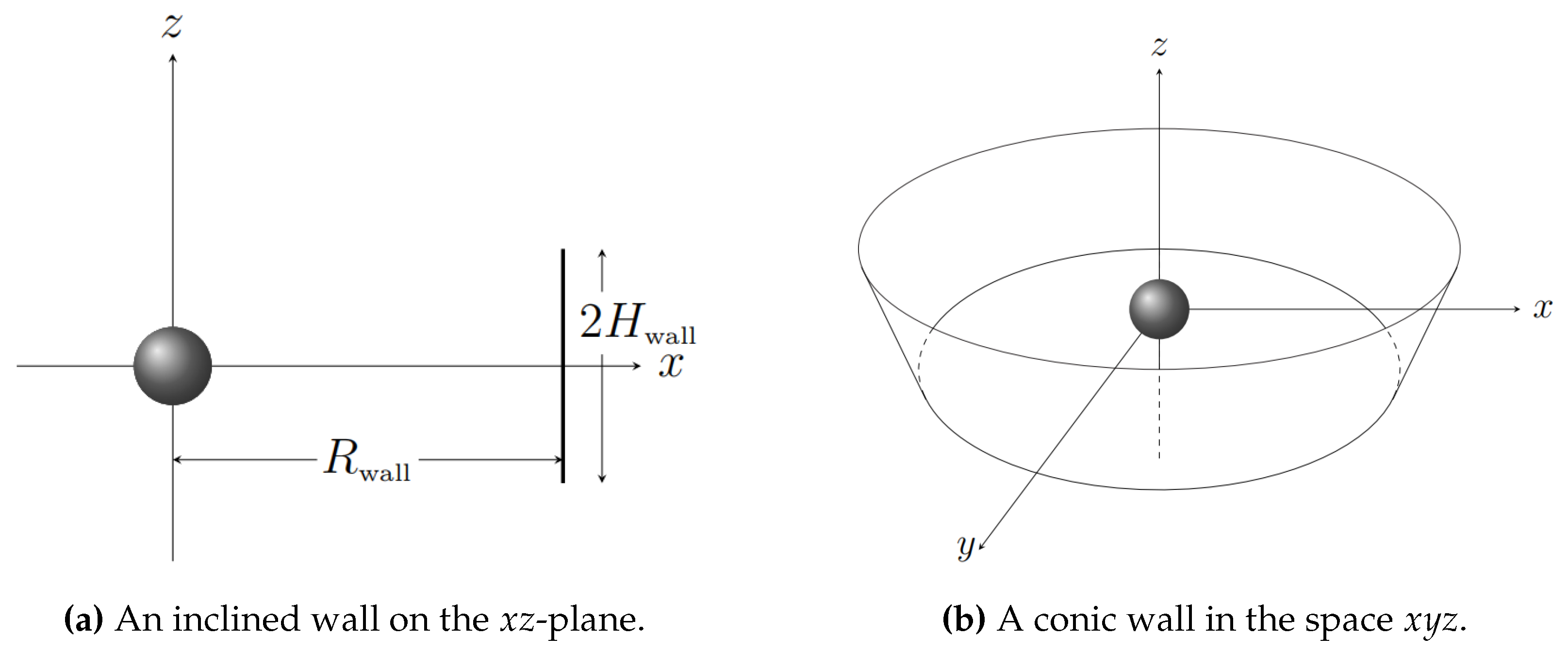
Figure 2.
Schematic representation of the visible surface of the wall as seen by the observer for two inclination angles.
Figure 2.
Schematic representation of the visible surface of the wall as seen by the observer for two inclination angles.
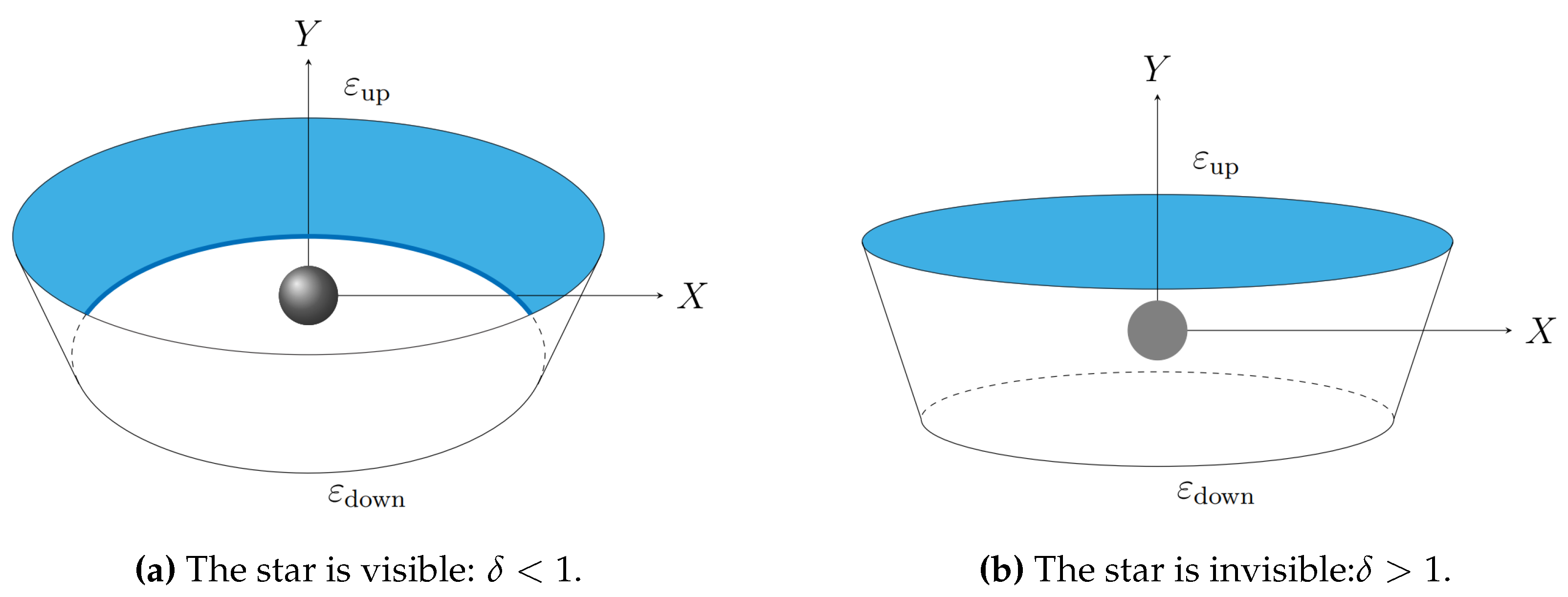
Figure 3.
Geometry of the visible wall projected on the plane of the sky for two inclination angles.
Figure 3.
Geometry of the visible wall projected on the plane of the sky for two inclination angles.
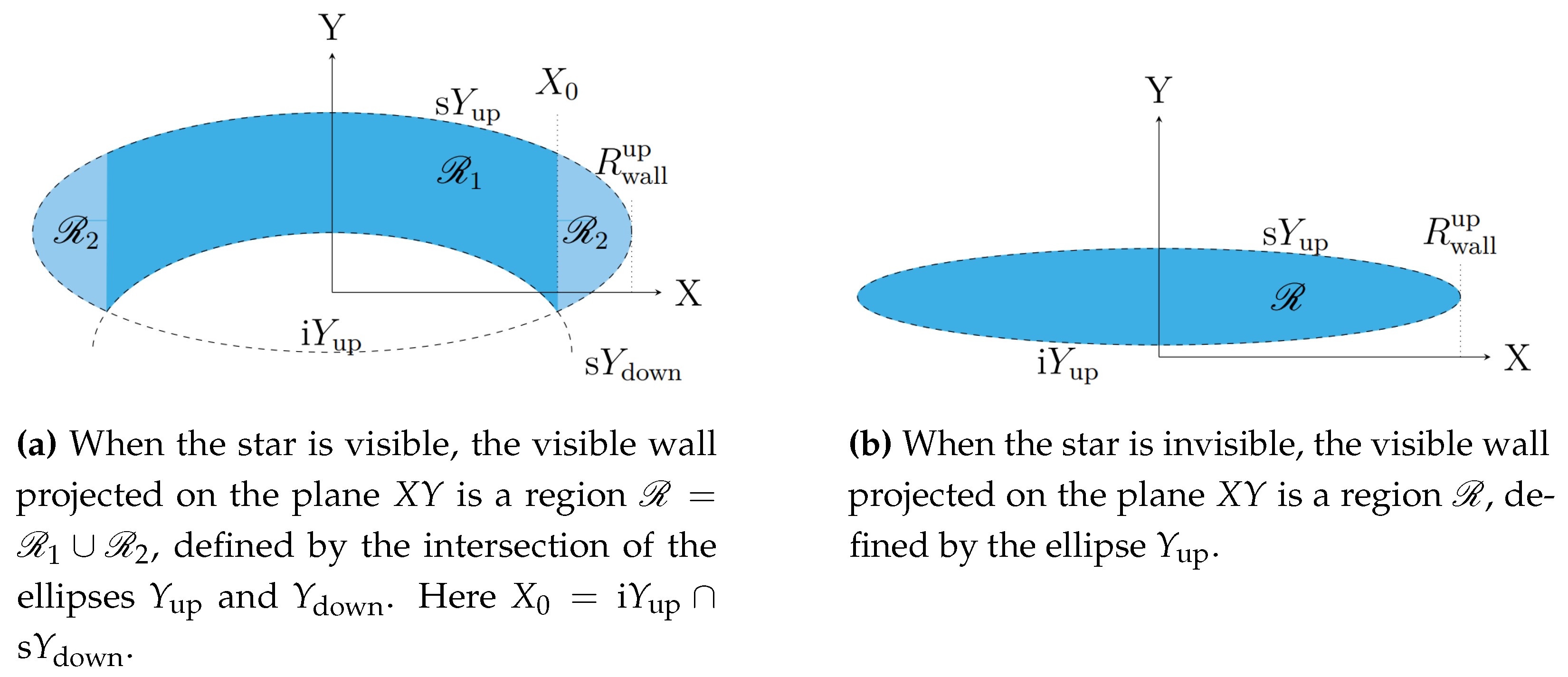
Figure 4.
Construction of a tri–dimensional vertical wall.
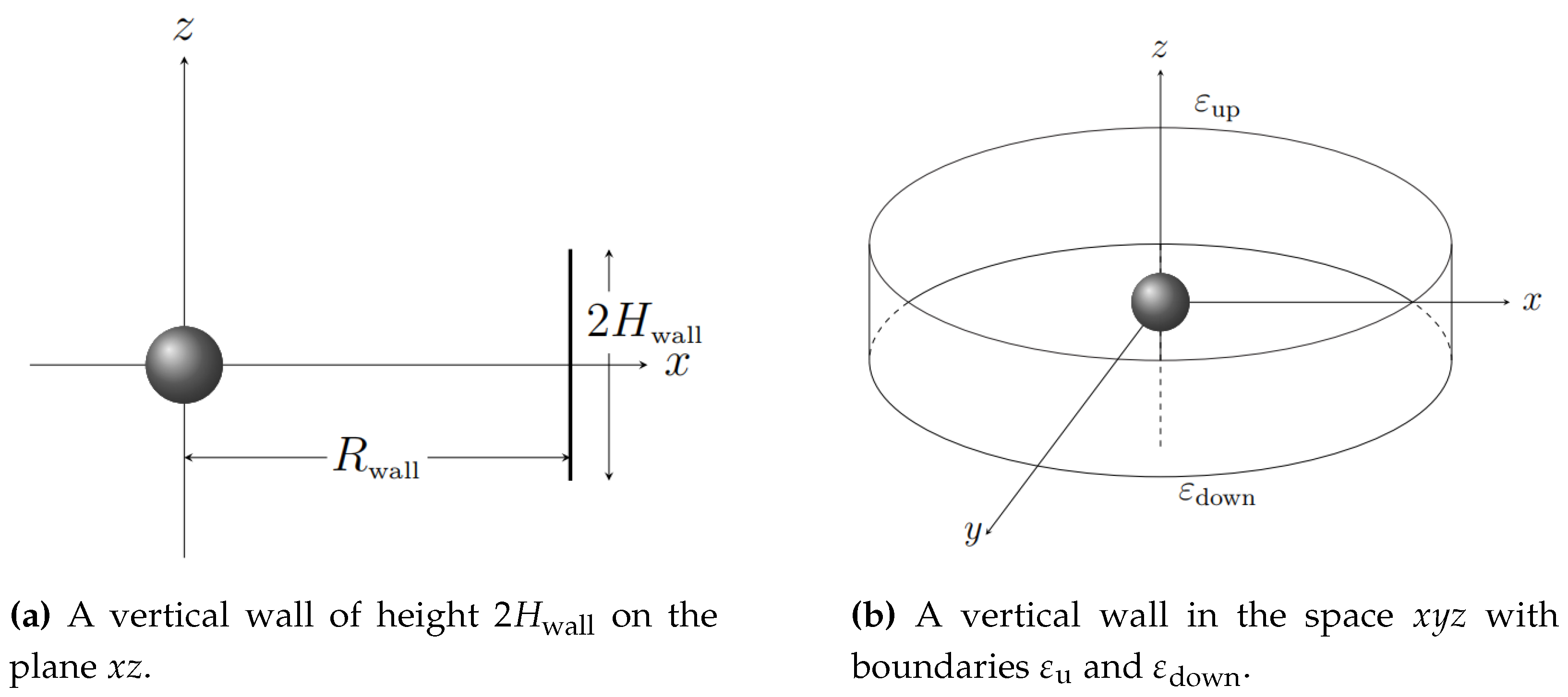
Figure 5.
Geometry of the incidence of the stellar radiation along a ray on the wall .
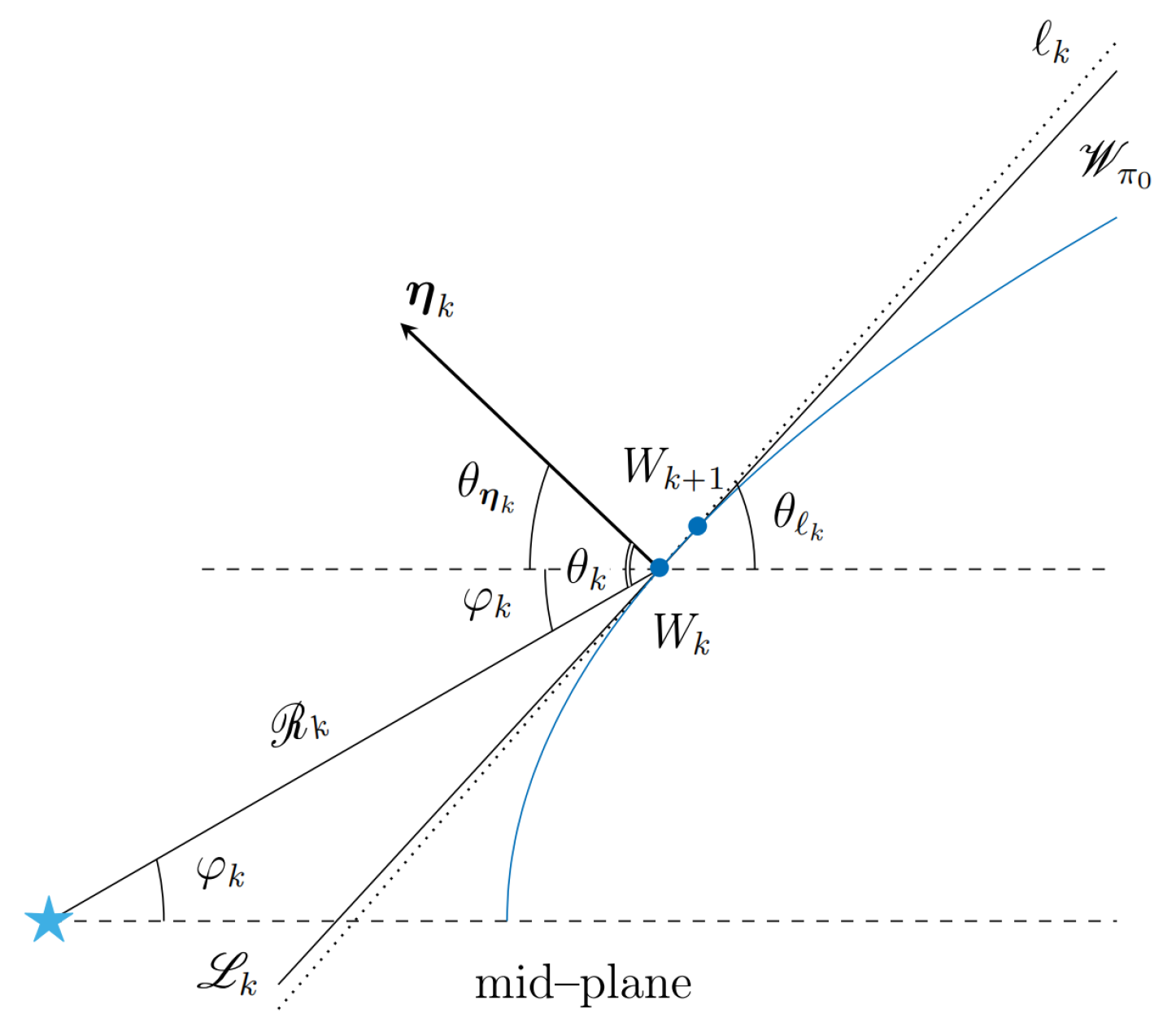
Figure 6.
Discretization of a two–dimensional curved wall by inclined line segments , for , and one vertical wall with in height.
Figure 6.
Discretization of a two–dimensional curved wall by inclined line segments , for , and one vertical wall with in height.
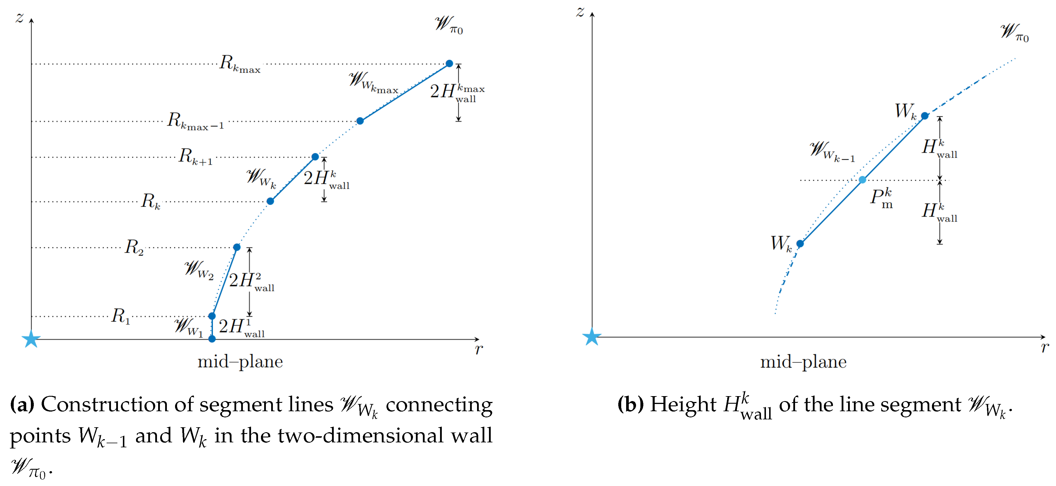
Figure 7.
Construction of a tri–dimensional wall : Each couple of points and in the two–dimensional wall defines a ring .
Figure 7.
Construction of a tri–dimensional wall : Each couple of points and in the two–dimensional wall defines a ring .
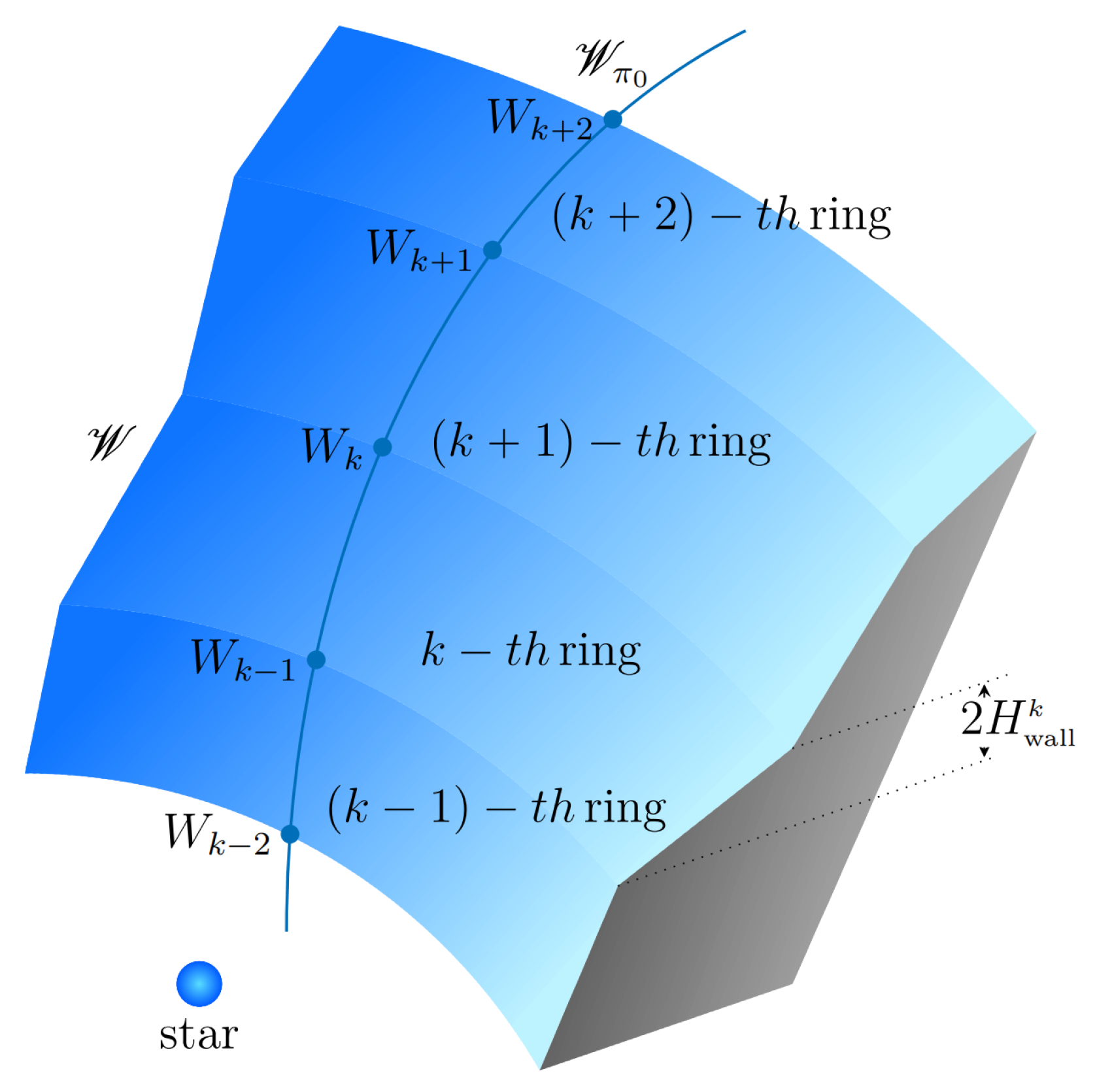
Figure 8.
Projection of a ring on the Y-axis: When the ring is located at distance along the z-axis of the system , the projected distance on the Y-axis is .
Figure 8.
Projection of a ring on the Y-axis: When the ring is located at distance along the z-axis of the system , the projected distance on the Y-axis is .
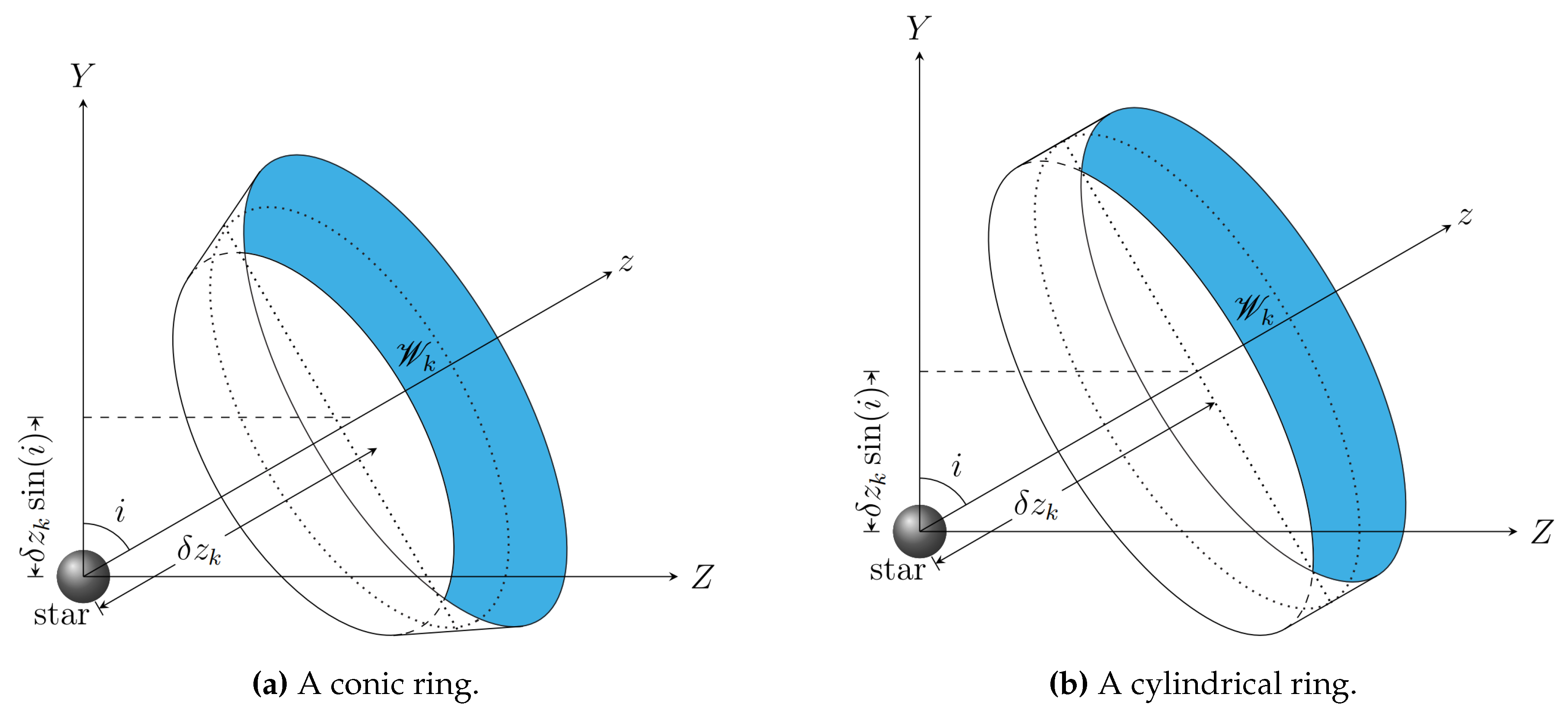
Figure 9.
A flow chart of the rhadamante code.
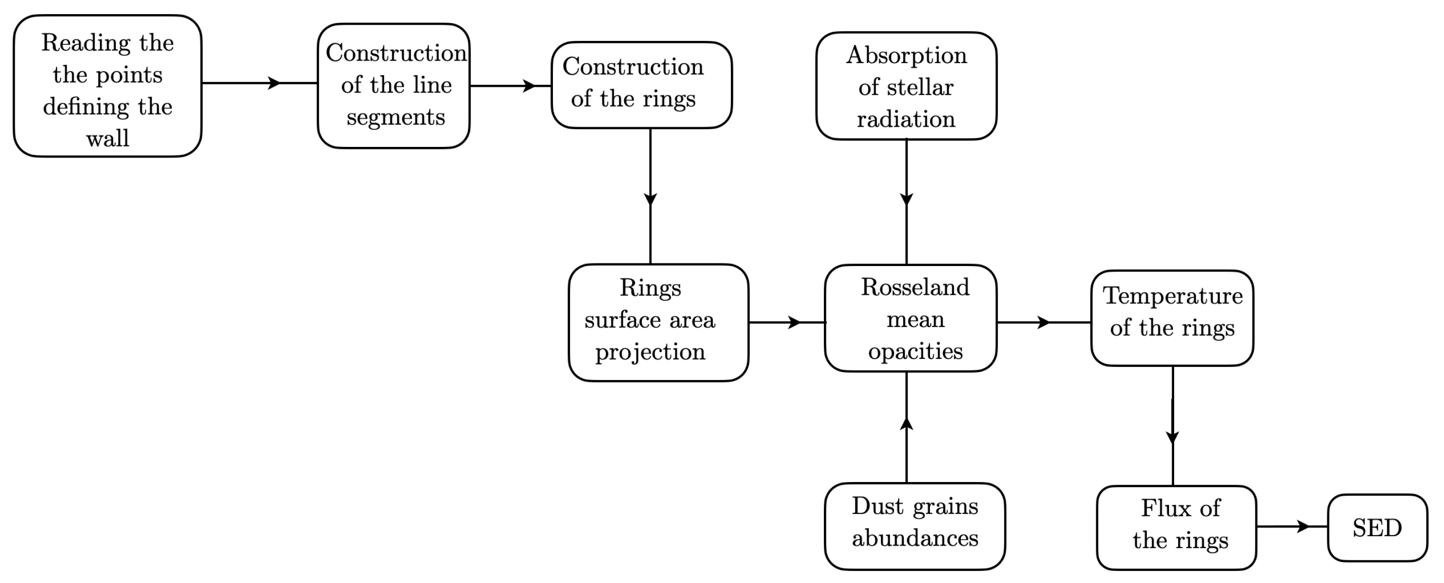
Figure 10.
Visualization of the 3D simulation (100 orbit).
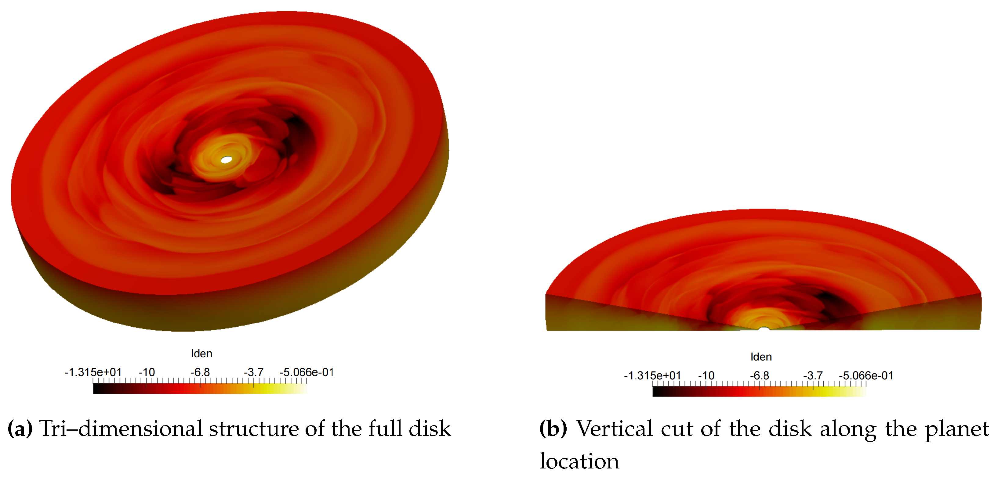
Figure 11.
Density isocontours on the disk: Gap opening.
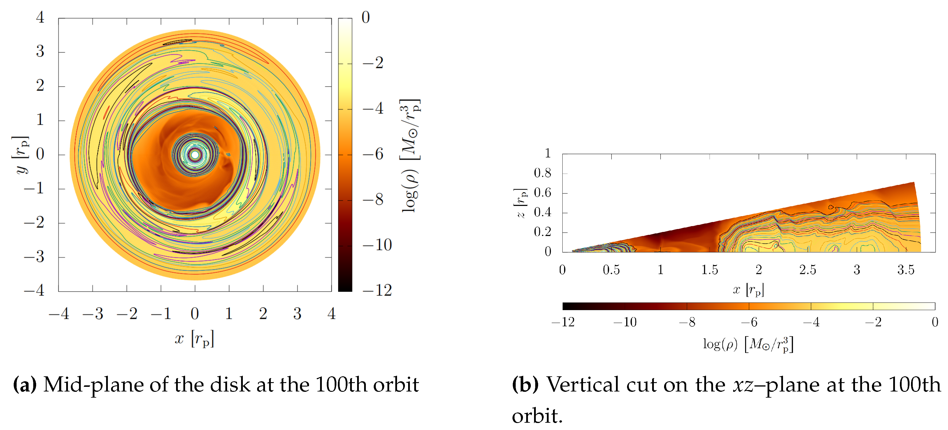
Figure 12.
Vertical geometry of the wall of the inner edge of the outer disk (picture is not scaled proportionally): Because of the embedded planet the wall is curved. It is ∼ in width and ∼ in height. In this model, the dust consists of a mixture of small and big grains of glassy olivine (silicate) with 50%Fe and 50% Mg and with a small amount of organic and troilite grains.
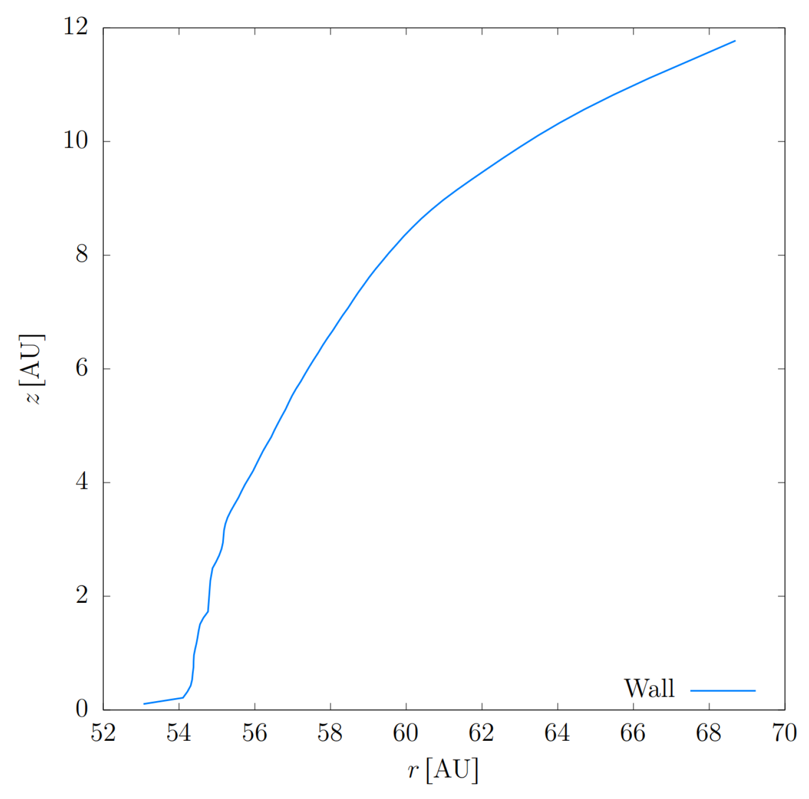
Figure 13.
Schematic representation of the pre-transitional disk LkCa15. In this ilustration the blue point represents the central star and the curved lines are the disk walls. The wall of the inner disk is fully illuminated by the central star. For the wall of the outer disk, light blue line represents the portion of the wall that is fully illuminated by the star, and black corresponds to the part of the wall that is in the umbra of the inner disk.
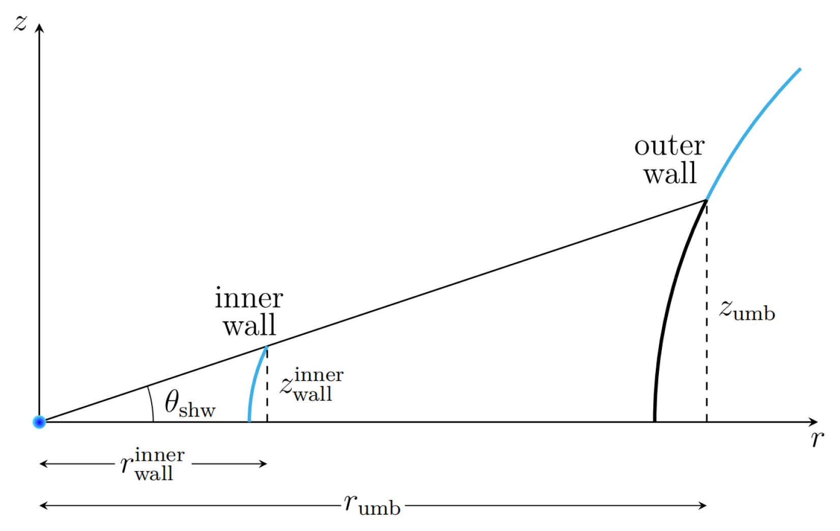
Figure 14.
Area of the projection of a curved wall on the plane of the sky . The wall starts at along the mid-plane and ends at , with total height of , and the disk inclination angle is .
Figure 14.
Area of the projection of a curved wall on the plane of the sky . The wall starts at along the mid-plane and ends at , with total height of , and the disk inclination angle is .
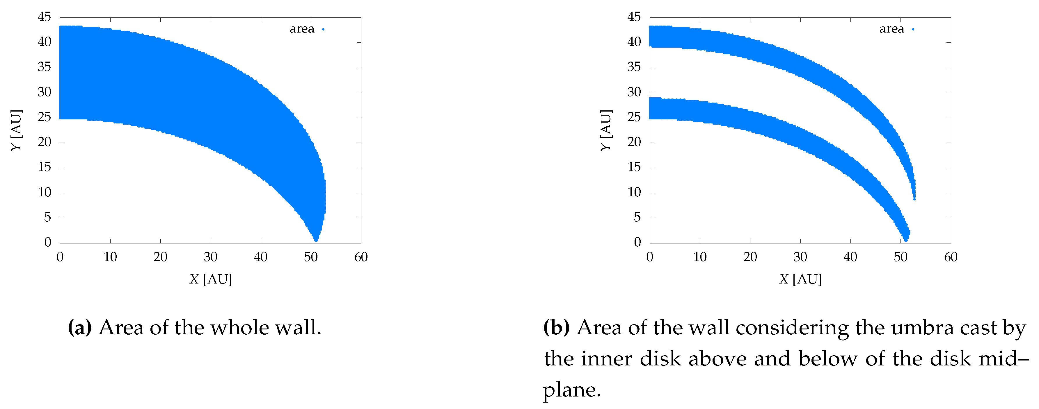
Figure 15.
Examples of wall synthetic SEDs (green line) compared to the observed SED (blue line) of LkCa 15. The dust mixture consists of different chemical composition of glassy pyroxene silicate grains and with a small amount of organic and troilite grains.
Figure 15.
Examples of wall synthetic SEDs (green line) compared to the observed SED (blue line) of LkCa 15. The dust mixture consists of different chemical composition of glassy pyroxene silicate grains and with a small amount of organic and troilite grains.
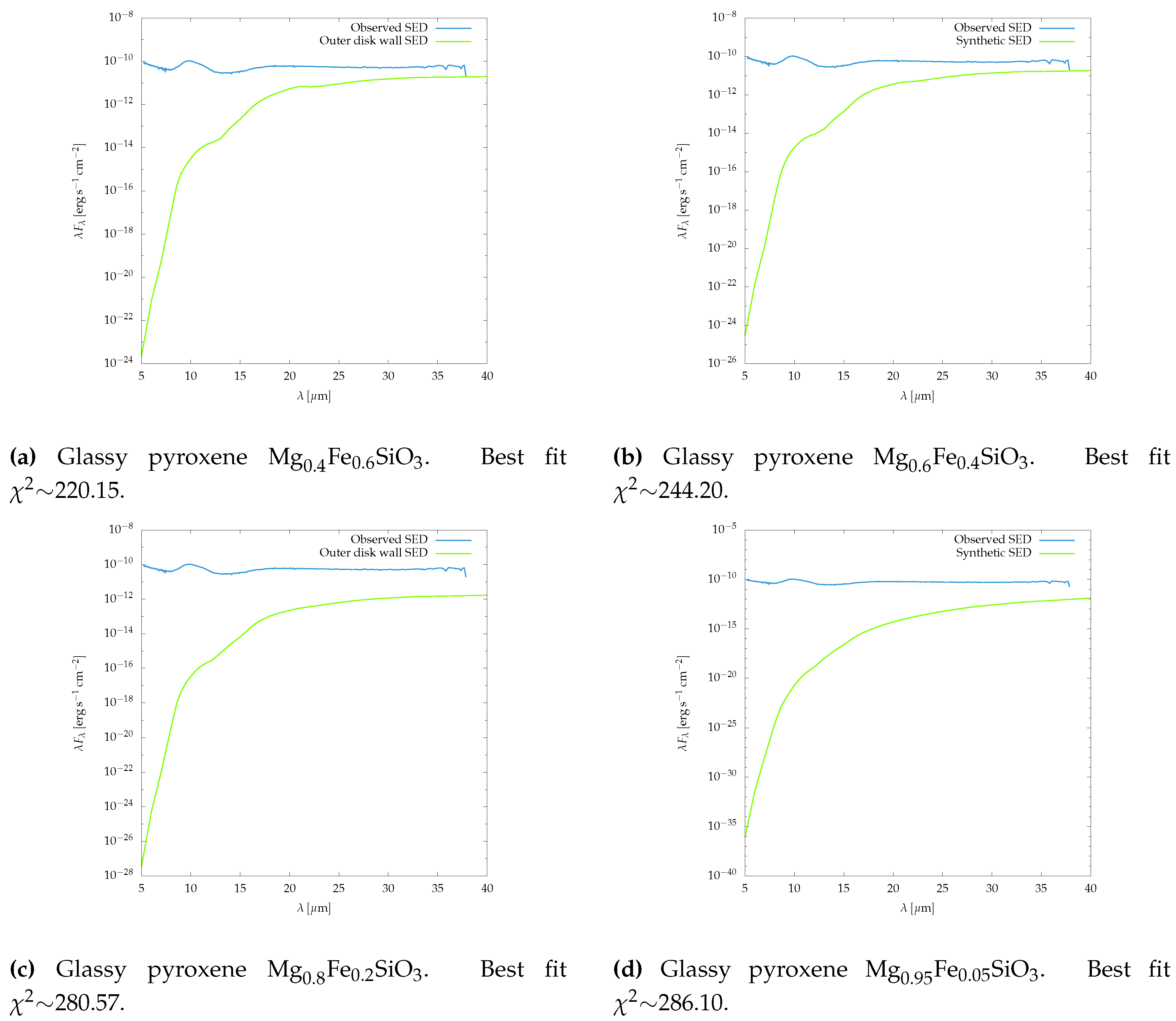
Figure 16.
Examples of wall synthetic SEDs (green line) compared to the observed SED (blue line) of LkCa 15. The dust mixture consists of different chemical composition of glassy olivine silicate grains and with a small amount of organic and troilite grains.
Figure 16.
Examples of wall synthetic SEDs (green line) compared to the observed SED (blue line) of LkCa 15. The dust mixture consists of different chemical composition of glassy olivine silicate grains and with a small amount of organic and troilite grains.
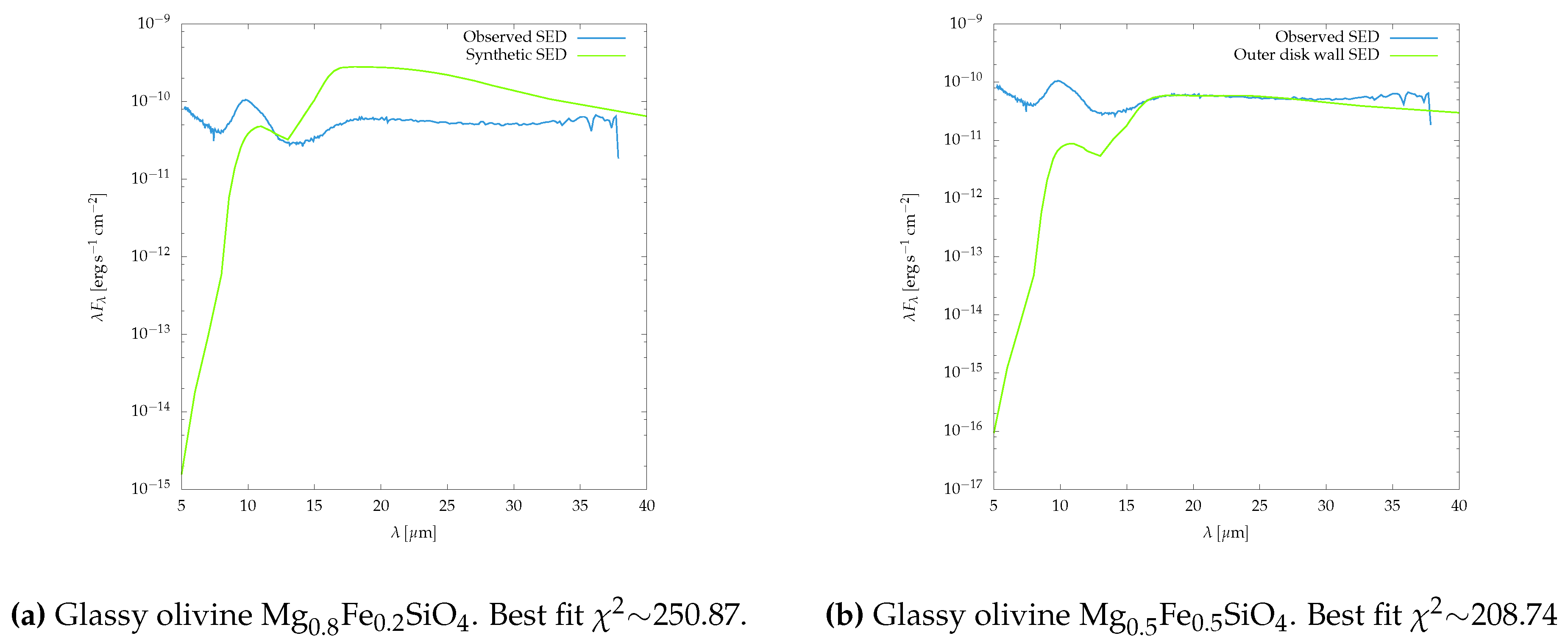
Figure 17.
Pre-transitional disk model of LkCa 15. The best-fit model to LkCa 15 (dark blue line), with a ∼ gap, consists of an inner optically thick disk with a curved sublimation wall and an outer optically thick disk with a curved wall. Separate model components are the stellar photo-sphere (yellow line), the inner disk sublimation wall (magenta line) and the outer disk wall (green line). We show the Spitzer IRS SED (light blue line).
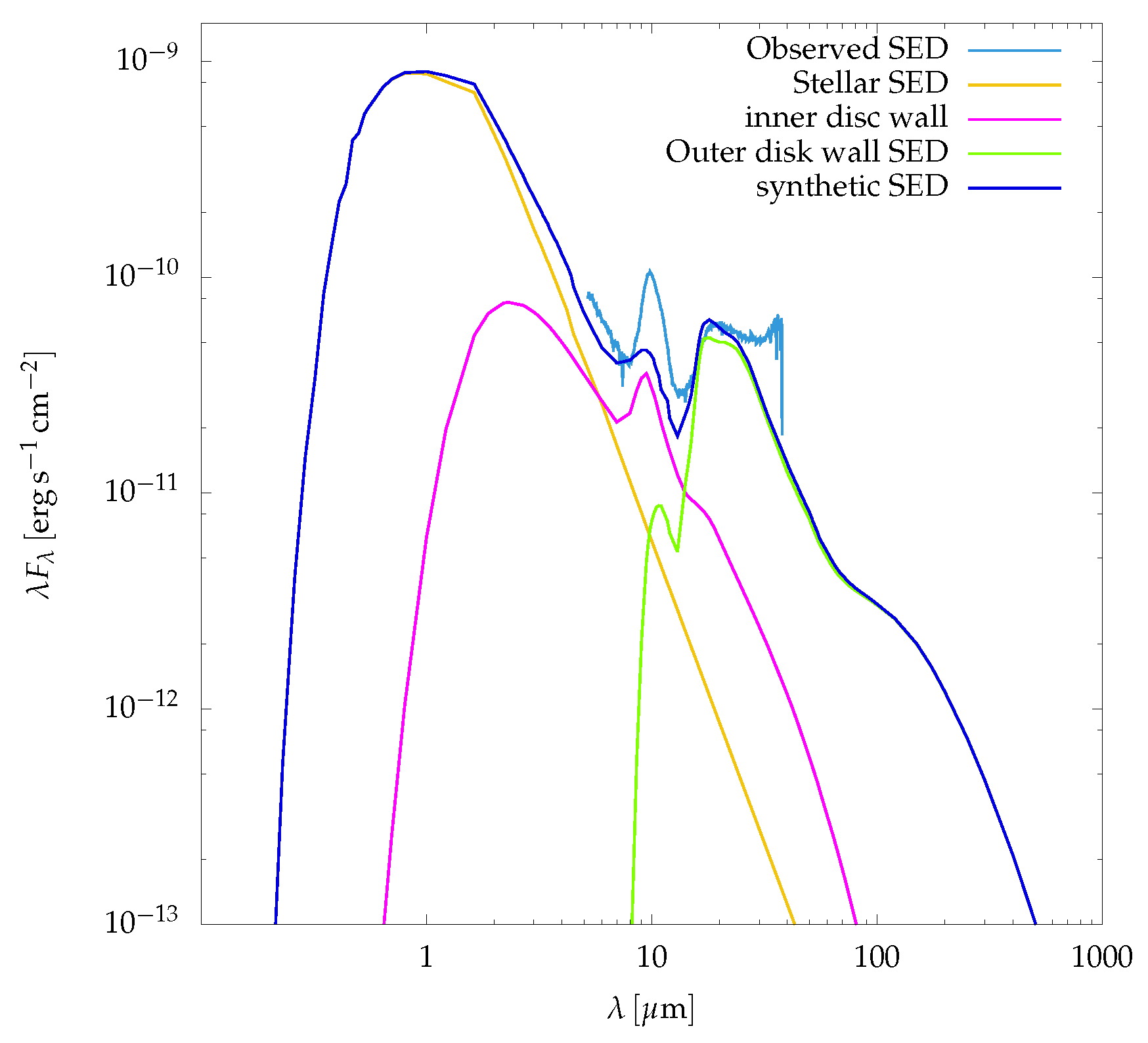
Figure 18.
Synthetic SED (green line) that best fit the observed SED (blue line) of LkCa15. With model parameters: , , , . The dust in the inner disk consists of small grains () and big grains () of silicates and graphite, while in the outer disk, the dust consists of small ( and ) and big grains (, ) of glassy olivine with 50% Fe and 50% Mg and with a small amount of organic and troilite grains.
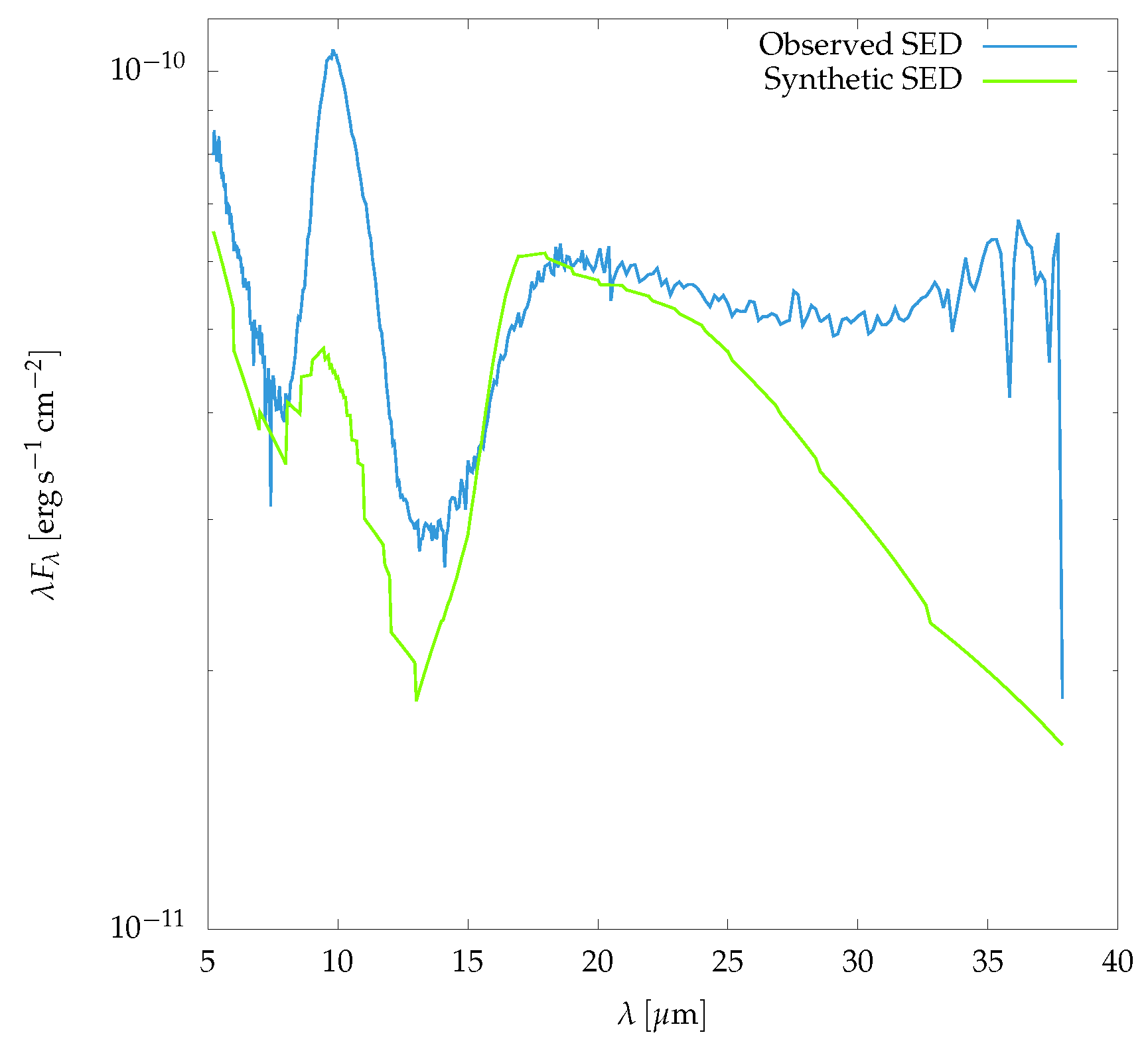
Figure 19.
Comparison between synthetic SEDs of vertical walls of gaps located at different , and a curved wall starting at and finishing at , created by rhadamante code. All the walls are in height, and it is considered a shadow (umbra) on the walls of due to the inner disk. Spitzer IRS SED is showed in blue.
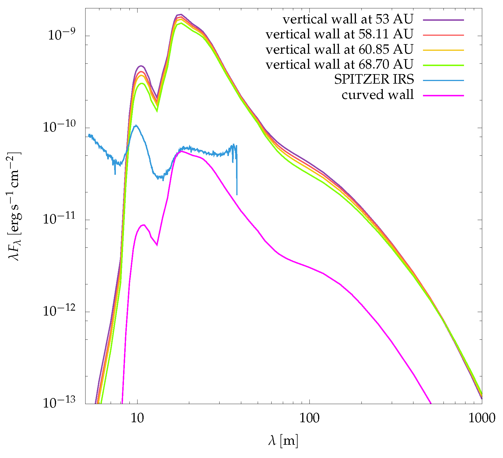

Table 1.
Disk-planet simulation specifications.
| parameter | value | |
|---|---|---|
| Disk | Aspect ratio H | |
| Surface density | ||
| –viscosity | ||
| slope | 1.0 | |
| Flaring index | 0.0 | |
| Planet | ||
| RocheSmoothing | 0.4 | |
| Acretion | No | |
| Mesh | Units | unitless |
| Dimension | 3D | |
| Geometry | spherical | |
| Timing | Orbits | 500 |
Table 2.
Parameters of the wall for different chemical composition of silicate dust grains: pyroxene and olivine. Organic and troilite grains composition is the same for all cases.
Table 2.
Parameters of the wall for different chemical composition of silicate dust grains: pyroxene and olivine. Organic and troilite grains composition is the same for all cases.
| silicate | [AU] | [AU] |
|---|---|---|
| pyroxene | ||
| 56.0 | 11.5 | |
| 49.8 | 12.3 | |
| 51.0 | 12.0 | |
| 50.0 | 13.2 | |
| olivine | ||
| 52.5 | 10.0 | |
| 53.0 | 12.0 | |
Table 3.
Stellar and model properties: and in the case of the outer wall are measured at the location of the umbra cast by the inner disk. Olivine silicate grains composition is 50% Fe and 50% Mg.
Table 3.
Stellar and model properties: and in the case of the outer wall are measured at the location of the umbra cast by the inner disk. Olivine silicate grains composition is 50% Fe and 50% Mg.
| parameter | value | |
|---|---|---|
| Star | 4370 K | |
| Disk | Inclination | |
| Inner wall | ||
| Dust | silicates | |
| graphite | ||
| Outer wall | ||
| Dust | olivine | |
| organics | ||
| troilite |
Disclaimer/Publisher’s Note: The statements, opinions and data contained in all publications are solely those of the individual author(s) and contributor(s) and not of MDPI and/or the editor(s). MDPI and/or the editor(s) disclaim responsibility for any injury to people or property resulting from any ideas, methods, instructions or products referred to in the content. |
© 2024 by the authors. Licensee MDPI, Basel, Switzerland. This article is an open access article distributed under the terms and conditions of the Creative Commons Attribution (CC BY) license (http://creativecommons.org/licenses/by/4.0/).
Copyright: This open access article is published under a Creative Commons CC BY 4.0 license, which permit the free download, distribution, and reuse, provided that the author and preprint are cited in any reuse.


