
Submitted:
05 November 2024
Posted:
07 November 2024
You are already at the latest version
Abstract
Considering the sustained increase of dengue outbreaks in Latin America in recent years, this study proposes the use of machine learning (ML) tools with epidemiological data, meteorological climate parameters considering El Niño and La Niña (Niño 3.4 Index), and socioeconomic and demographic phenomena as a basis for the construction of an early warning system for dengue outbreaks in Zulia State, Venezuela. The study area covers 21 municipalities. Two ML models, support vector regression machine (SVM-R) and Gaussian process regression (GPR), were used. The data were used raw, standardised, and normalized for each model to be trained. The predictions of dengue outbreaks from the GPR and SVR algorithms show agreement with the dates of the real data; it was determined that there is a range of 2 to 3 weeks depending on the municipality. These coincide with previous studies showing that the algorithms do not work properly for some municipalities.
Keywords:
Dengue
; machine learning
; epidemiology
; global
; forecast
Introduction
Dengue fever is a vector-borne disease that has become endemic in tropical and sub-tropical regions worldwide over the last century and now poses a threat to half of the world´s population [1], Aedes mosquitoes, the species responsible for the dengue transmission, are now found in more than 130 countries making dengue the single most significant human disease burden of any arbovirus with around 10.000 deaths and more than 100 million symptomatic infections per year [1,2]. This grim global scenario is exacerbated by other Aedes-like species reported in many parts of the world, coupled with factors such as migratory displacement, political conflict, climate change, unplanned urbanisation and inefficient public services [2].
In this context, the Neglected Tropical Diseases (NTDs) initiative, established as part of the United Nations Sustainable Development Goals (SDGs) in 2015 to address the global challenges of dengue fever and other infectious diseases, emphasises the necessity of a multidisciplinary approach to dengue eradication, requiring an unprecedented level of cooperation and collaboration between different sectors [3].
In the case of dengue in Venezuela, it has shown sustained increases, both in the interannual magnitude of cases and in the frequency of outbreaks [4]. In this regard, six major dengue epidemics were documented in Venezuela between 2007 and 2016 [5]. The largest was in 2010, the third largest ever recorded in the Americas, with a peak of about 1,000,000 cases, of which more than 10,000 were severe[5]. Zulia state is one of the most affected regions, as shown in Figure 1. In this regard, recent spatio-temporal models of dengue in Zulia state using Generalized Additive Mixed models [6] suggest the need for urgent intervention there to improve certain living conditions of the inhabitants, as a way to reduce the growing escalation of dengue in that part of the country.
Likewise, the World Health Organization (WHO) has stated that the prediction of dengue outbreaks is one of the main objectives for effective public global health [8,9]; and Machine Learning (ML) techniques are a promising approach for epidemiological studies [10], that can provide for knowledge of dengue outbreaks, with the aim of the development of Early Warning Systems (EWS) to control the disease [8,10,11,12,13,14].
Based on the above, the main objective of this study is to evaluate the possibility of creating an Early Warning System for Dengue Prevention in Venezuela appropriate for the local environment of Zulia State using climatic data in conjunction with socioeconomic and demographic data. Using the algorithms Support Vector Regression (SVR), which is an extension of Support Vector Machines (SVM) applied to regression problems[15,16]; and the Gaussian Process Regression (GPR) is a non-parametric supervised learning method used to solve regression and probabilistic classification problems[17,18].
Preliminaries
The typical of these studies is that the authors use climate variables as predictors of dengue incidence using the Generalized Additive Model for Location, Scale, and Shape (GAMLSS) and Random Forest (RF). In this [8], the authors applied Vector Auto Regression (VAR), Generalized Boosted models (GBM), Support Vector Regression (SVR), and Long Short-Term Memory (LSTM) to predict dengue prevalence using meteorological data. In [14] the authors used climate data to train a Support Vector Machine (SVM) classifier with Radial Basis Function (RBF) kernel; In [19], the authors compared LSTM time series forecasting for dengue prediction with Support Vector Regression (SVR).
A study performed in China [20] for instance, used weekly data since 2011-2014 in conjunction with meteorological factors with appropriated delayed effects plus Internet search engine query statistics to construct predictive models of dengue. Several models were tried to compare and identify the optimal performance through Goodness of Fit validation of Root Mean-Square Error (RMSE) and R-squared measures.
In [21] the authors perform a systematic review of ML techniques applied to the study of dengue, creating a list of the most common ML regression models for predictive applications. Similarly, in [19] a review of ML models used to estimate possible dengue outbreaks was carried out. The diagram in Figure 2 shows some of the most used ML models for dengue outbreak forecast studies.
The study performed in China [20] considered a delayed climatic factor effect identified through a Cross-Correlation Analysis, the obtained results were: The Nino 3.4 with 2 months lag; mean temperature at 3 months lag; soil moisture at 1-month lag and both rainfall and relative humidity with a 0-month lag.
Another study performed in India [8] confirmed those values, but also found the most significant lagged terms of the Nino3.4 with 2-month lag, mean temperature with 3- months lag, soil moisture with 1-month lag, rainfall and relative humidity with zero-month lag respectively.
Methods
Study Area
This study used data related to Zulia state, which is located in the northwest part of Venezuela, between 8.20° to 11.79° North latitude and between 70.73° and 73.37° West longitude [6]. The state is divided into 21 municipalities, covering 50,230 square kilometers around Lake Maracaibo. These municipalities (Figure 3) are: Almirante Padilla, Baralt, Cabimas, Catatumbo, Colon, Francisco Javier Pulgar, Jesús Enrique Lossada, Jesús María Semprún, La Cañada de Urdaneta, Lagunillas, Machiques de Perijá, Mara, Maracaibo, Miranda, Indígena Bolivariano Guajira, Rosario de Perijá, San Francisco, Santa Rita, Simón Bolívar, Sucre and Valmore Rodríguez.
Data Integration
A series of data (Figure 4) from various sources, such as epidemiological data, socioeconomic and demographic data, and local and local climatic data, were integrated for this study. The characteristics of these data are presented as follows.
Epidemiological Data
Hospital admissions of dengue fever were provided by the Venezuelan Ministry of Health as weekly reported dengue fever cases from January 2008 to December 2016. A case was operationally defined as hospital admission, regardless of disease severity. This study is similar to a previous one performed in Zulia State by Cabrera M & Taylor G[6], framed on an overall dengue admission rate and range across the Zulia state municipalities.
Climate and Weather Data
Meteorological data from Zulia state was obtained from NASA Earth Science's Applied Program’s POWER (Prediction Of Worldwide Energy Resources) project [22]. This project provides NASA's solar and meteorological data sets to support renewable energy schemes, building energy efficiency and agricultural needs. Meteorological parameters are achieved from NASA's GMAO MERRA-2 assimilation model plus GEOS-5.12.4 FP-IT. The Data Access Viewer was used to search the geographical coordinates across the zone: -74° West to -70° East and 12° North to 8° South (Lat 10.6417 Long -71.6295) [22] using the following meteorological parameters:
- Temperature at 2 Meters Maximum (°C)
- Temperature at 2 Meters Minimum (°C)
- Specific Humidity at 2 Meters (g/kg)
- Relative Humidity at 2 Meters (%)
- Precipitation Corrected (mm/day)
- Wind Speed at 2 Meters (m/s)
- Wind Speed at 2 Meters Maximum (m/s)
Since meteorological conditions in Venezuela are heavily influenced by El Niño producing warmer temperatures and reduced precipitation, and La Niña with the opposite effect - cooler temperatures and more significant rainfall [4] we used the Niño3.4 Index, following earlier Venezuelan studies [4,6]. The Niño 3.4 index was obtained from the National Oceanic and Atmospheric Administration (NOAA) [23].
Socio-Economic and Demographic data
While multiple factors contribute to dengue incidence, the collection of socioeconomic data in the Zulia state is restricted by the limited information recorded in the 2011 census conducted by the National Institute of Statistics due to the lack of available data for the country. In this regard, the socioeconomic variables within this category were aggregated at the municipality level in Zulia, as provided by the 2011 Census. These variables included the proportion of households living in poverty and the proportion with access to piped water supply.
Regarding demographic data, the annual population figures were obtained from INE (2014), also based on the Venezuelan National Census of 2011. These figures were used to address gaps in demographic data from 2008 to 2016, aggregated at the municipality level. These gaps arose due to the absence of formal population surveys the Venezuelan national government conducted since 2011. Therefore, the most recent population size data available for the municipalities in Zulia state is from 2011. While this decision may limit the results, it represents the most accurate approximation.
Machine Learning Algorithms
In this study, it was decided to use the Support Vector Regression (SVR) algorithm, which is fundamentally the Support Vector Machine (SVM) algorithm for regression, since it is one of the most widely used algorithms in Dengue studies, as previously mentioned. It was decided to use Gaussian process regression (GPR) because there are only a small number of previously published studies using this algorithm [24,25] applied directly to dengue and in the case of Venezuela there are no previous studies. A summary of these algorithms is presented below.
Support Vector Machine (SVM):
This technique, devised in the 1960s and substantially improved in the 1990s, is based on statistical learning theory and the principle of structural risk minimisation [15,16]. SVM-Regression (SVM-R) has become a prevalent technique for dengue prediction [15] due to its reported efficiency in generalization performance [16]. As a predictor tool it has shown excellent empirical results by maximising predictive accuracy and avoiding overfitting [15]. SVM-R includes three major components to be considered: (i) learning theory; (ii) optimal hyperplane algorithm and (iii) kernel functions [15].
We briefly examined all three primary kernel functions but settled on the RBF as the most effective one (Table 1).
According to specialists, no efficient, structured method for selecting the optimal hyperparameters exists. Therefore, a simple approach is used to optimise one parameter at a time [15]. Hence, the evaluation of parameters of for instance, with a fixed parameter C at value 1.0, through a wide range of (typically) exponential forms: is tried. Once the optimal value has been found, the optimal value of parameter C is determined [15].
Gaussian Process Regression
Gaussian process regression (GPR) [18] is a regression approach gaining significant attention in Machine Learning [26,27,28], due to its nonparametric and Bayesian characteristics. This methodology has shown remarkable performance with small datasets and its ability to provide uncertainty measurements on the predicted outcomes. In contrast to many widely used supervised Machine Learning algorithms that strive to learn precise values for each parameter in a given function, the Bayesian approach takes a different path by inferring a probability distribution across all potential values.
Let the training set , where and , obtained from an unknown distribution. A GPR model addresses the question of predicting the value of a response variable , given the new input vector , and the training data [29]. A linear regression model is of the form:
Where:
, with σ2 the error variance and the coefficients β are estimated from the data.
A GPR model uses latent variables and explicit basis functions to explain the response. The covariance function captures the latent variables, and the basis functions project the inputs into a p-dimensional feature space.
A Gaussian Process (GP) is a collection of random variables in which any finite number follows a joint Gaussian distribution[30]. If is a GP, then given n observations , the joint distribution of the random variables is Gaussian; characterised by its mean function and covariance function , that is:
Now consider the following model.
where:
- ○
- ,
- ○
- : are a set of basis functions that transform the original feature vector into a new feature vector .
- ○
- : is a p-by-1 vector of basis function coefficients.
This model represents a GPR model. An illustration of response can be modeled as
Therefore, a GPR model is a probabilistic model. A latent variable is introduced for each observation xi, making the GPR model nonparametric. In vector form, the GPR model can be written as follows:
where:
The joint distribution of latent variables ) in The GPR model has the following form:
approach to a linear regression model, where is in the following form:
The covariance function is usually written as to explicitly indicate the dependence on ; because it is generally parameterised by a set of kernel parameters or hyperparameters . Now, the kernel parameters are based on the signal standard deviation and the characteristic length scale . The determination of characteristic length scale serves to delineate the separation between input values at which the response values are rendered uncorrelated. Both and require to be greater than 0, and this can be enforced by the unconstrained parameterization vector θ, such that:
Squared Exponential Kernel
Matern 5/2
Rational Quadratic Kernel
Where:
ARD Exponential Kernel
ARD Matern 3/2
where:
The methodology applied in the present study used dengue cases in Zulia state weekly aggregated in conjunction with a set of socioeconomic and local and global climatic variables and based on previously implemented machine learning algorithms used for other parts of the world [8,15,20]. The construction of Support Vector Regression (SVR) and Gaussian process regression (GPR) as traditional ML algorithms were performed due to their flexibility, practicality and typically excellent performance. A set of scenarios was proposed in the models for comparative purposes using both climatic and non-climatic factors and respective validations to obtain the optimum model. Figure 5 shows the process implemented in this study.
Data Integration: Various preliminary steps were used to prepare the data before being entered into the machine learning algorithms:
- Weekly epidemiological data of dengue cases in Zulia state were aggregated at the municipal level in conjunction with a set of climatic and non-climatic covariants. In this context it was necessary to integrate the existing data because of the different sources of information (as proposed Cabrera M & Taylor G. [6]). The present study also utilised remote satellite climatic data obtained from NASA as described previously.
- Epidemiological data was missing for Guajira municipality between 2013 to 2016, which resulted in this municipality being excluded from the study.
- Some demographic data, such as 2008 and 2016, had 53 weeks due to the day the new year started, whilst the climatic data was always divided into 52 weeks. This was dealt with straightforwardly by repeating the previous week´s climatic data for the 53rd week where this occurred. The Niño 3.4 index was aggregated at a weekly level to be consistent with the other data.
- According to some authors [15], the data can be sensitive to extreme values. Therefore, in some cases, it is convenient to normalize or standardize the data. In this study, raw, standardized, and normalized data were used for each model to be trained. In this way, choose the best model obtained. In Standardization: the software centers and scales each column of the predictor data according to the mean and standard deviation of the column. In Normalization: it scales each column of the predictor data between -1 and 1.
Model Construction: Two different machine learning algorithms were used for comparative purposes in this study, chosen for their reported accuracy in dengue forecasting in other parts of the world [8,15,20,32] .
To conduct the experiments, the MatLab Statistics and Machine Learning Toolbox [33] was used, which provides a framework for designing and implementing ML algorithms, and applications. The experiments were carried out with a PC Laptop of the following characteristics: CPU Intel(R) Core(TM) i7-10750H CPU @ 2.60GHz, 12,0 GB RAM, GPU NVIDIA GeForce RTX2060 with Max-Q design. We perform 10-fold cross-validation on the database aiming to obtain unbiased results in our experiments.
Fitting the GPR model requires estimating the following model parameters from the data:
- ○
- Covariance function parameterized in terms of kernel parameters in vector θ
- ○
- Noise variance
- ○
- Coefficient vector of fixed-basis functions β
Fitting the SVR model requires solves an optimization problem that involves two parameters:
- ○
- The regularization parameter C and
- ○
- The error sensitivity parameter ϵ.
Results
GPR outcomes
Once the data were integrated, we applied the GPR algorithm to the data. In this case we sought to optimize both the kernel functions and the hyperparameters. The results show that for each dataset the behavior is different, with the result that the algorithm works well for some municipalities whilst is unsatisfactory for others. This finding is consistent with results obtained from previous studies [10,34], who similarly found that the same ML algorithm applied to dengue case data works well for some regions (states, municipalities, etc.) but not for others. The models were also evaluated, considering the effect of climate data on the incidence of dengue cases.
The results showed a lag of between two and three weeks in the effect of climate on the incidence of dengue cases in the municipalities of Zulia state. Table 2 shows the municipalities where the prediction trend reproduces the behavior of the real data of the considered municipalities.
Figure 6 shows the prediction results along with the actual dengue cases in six of the municipalities; these cover weeks 377 to 470 in the dataset. In all plots, there is an outbreak of dengue cases approximately between weeks 410 and 430, as well as between the 400th and 420th weeks. It is also observed that the GPR model prediction shows a similar pattern compared to real values.
Those weeks correspond to the last 9 weeks of the year 2015 and the first 11 weeks of the year 2016, that is, from November 2015 to the end of March 2016. It can be observed that, except for the Baralt municipality, from approximately week 460 to week 470, which corresponds to the last 10 weeks of 2016, dengue cases tend to increase.
This is consistent with the fact that it is in the same period where the previous outbreak was detected. In this way, the model predicted possible dengue outbreaks based on the meteorological conditions.
SVR outcomes
The results for the SVR show almost exactly the same behavior as for the GPR. Similarly, for some municipalities, approximate values of the real behavior of the outbreaks are obtained, and for other municipalities, adequate results are not obtained. In both cases, they indicate the periods of increase of dengue cases and always with two or three weeks of lag with regards to the climate. Table 3 shows the municipalities where the prediction trend reproduces the behavior of the real data of the considered municipalities.
Figure 7 shows the prediction results along with the actual dengue cases in six of the municipalities; these cover weeks 377 to 470 in the dataset.
Discussion
Dengue continues to be a significant public health problem, especially in Latin America, where currently multiple countries presenting an epidemic situation in 2024, with more than 1 million cases just in two months, especially in Brazil. Understanding this epidemiology and developing prediction models is critical for control and surveillance in endemic countries of the region, including Venezuela. Venezuela is of deepening concern due to the country's current economic, political and social difficulties [5,35]. The economic crisis brought it with hyperinflation of 180.9% in 2015 and poverty levels that rose from 33.9% in the first half of 2015 to 82% in 2016 [35]. Consequently, a combination of poverty, socio-economic factors, precarious living conditions and a grossly deficient public services such as water and electricity are the main drivers for its ongoing crisis in dengue infections [5].
In addition, in terms of surveillance system, the Epidemiological bulletins established since 1938 in Venezuela suffered an interruption since 2007-2014, and ultimately the publication of healthcare indicators has wholly stopped since 2018, after sixty-three years of continuous activity [5]. The combination of all those factors has allowed the reemergence of infectious diseases that had been primarily eradicated [5,35]; as a result, the extreme damage to the health and welfare of its inhabitants is a matter that requires urgent actions [5].
As for predicting mosquito-borne diseases, a study [10] claims that no model could be completely effective, mainly because they cannot fit all the necessary conditions from the real world. According to these authors, significant constraints are the insufficient available data and the lack of open-source information, in conjunction with an unstructured and inadequate set of information, amongst other drawbacks.
The evaluation of time series data in prediction probably needs further theoretical work. The prediction quality is usually given in terms of the difference between observed and predicted values at each instant. However, this is not really what is required for disease prediction. What is usually needed is the identification of outbreak peaks, and the accuracy of their predicted magnitude is probably less important than the accuracy of predicting them. Knowing that a peak is coming is more important than predicting its size. Similarly, the accuracy of the timing of the peak and the amount of notice that the predictive tool gives is more important than precisely predicting the size of the peak.
Conclusions
This study provided results consistent with other studies in that the predictive models are tolerably accurate for some locations but not others. This is possibly due to critical but as yet undefined features that are not accurately incorporated into the model.
Author Contributions
- Maritza Cabrera.: Conceptualization, investigation, methodology, Writing – review & editing, supervision, Data curation, Formal analysis.
- José Naranjo-Torres.: investigation, methodology, Writing – review & editing, supervision, Software, Formal analysis.
- Ángel Cabrera: Formal analysis.
- Lysien Zambrano: Writing – review & editing, supervision, Software, Formal analysis.
- Alfonso J. Rodríguez-Morales: Writing – review & editing, supervision, Software, Formal analysis.
Funding
The current article processing charges (publication fees) were funded by the Facultad de Ciencias Médicas (FCM) (2-03-01-01), Universidad Nacional Autonoma de Honduras (UNAH), Tegucigalpa, MDC, Honduras, Central America (granted to Zambrano).
References
- Messina, J.P.; Brady, O.J.; Golding, N.; Kraemer, M.U.G.; Wint, G.R.W.; Ray, S.E.; Pigott, D.M.; Shearer, F.M.; Johnson, K.; Earl, L.; et al. The Current and Future Global Distribution and Population at Risk of Dengue. Nat Microbiol 2019, 4, 1508–1515. [CrossRef]
- Allan, R.; Budge, S.; Sauskojus, H. What Sounds like Aedes, Acts like Aedes, but Is Not Aedes? Lessons from Dengue Virus Control for the Management of Invasive Anopheles. The Lancet Global Health 2023, 11, e165–e169. [CrossRef]
- Raviglione, M.; Maher, D. Ending Infectious Diseases in the Era of the Sustainable Development Goals. Porto Biomedical Journal 2017, 2, 140–142. [CrossRef]
- Vincenti-Gonzalez, M.F.; Tami, A.; Lizarazo, E.F.; Grillet, M.E. ENSO-Driven Climate Variability Promotes Periodic Major Outbreaks of Dengue in Venezuela. Sci Rep 2018, 8, 5727. [CrossRef]
- Grillet, M.E.; Hernández-Villena, J.V.; Llewellyn, M.S.; Paniz-Mondolfi, A.E.; Tami, A.; Vincenti-Gonzalez, M.F.; Marquez, M.; Mogollon-Mendoza, A.C.; Hernandez-Pereira, C.E.; Plaza-Morr, J.D.; et al. Venezuela’s Humanitarian Crisis, Resurgence of Vector-Borne Diseases, and Implications for Spillover in the Region. The Lancet Infectious Diseases 2019, 19, e149–e161. [CrossRef]
- Cabrera, M.; Taylor, G. Modelling Spatio-Temporal Data of Dengue Fever Using Generalized Additive Mixed Models. Spatial and Spatio-temporal Epidemiology 2019, 28, 1–13. [CrossRef]
- Gutiérrez, L.A. PAHO/WHO Data - Venezuela - Dengue Cases | PAHO/WHO Available online: https://www3.paho.org/data/index.php/en/mnu-topics/indicadores-dengue-en/dengue-subnacional-en/576-ven-dengue-casos-en.html (accessed on 12 June 2024).
- Kakarla, S.G.; Kondeti, P.K.; Vavilala, H.P.; Boddeda, G.S.B.; Mopuri, R.; Kumaraswamy, S.; Kadiri, M.R.; Mutheneni, S.R. Weather Integrated Multiple Machine Learning Models for Prediction of Dengue Prevalence in India. Int J Biometeorol 2023, 67, 285–297. [CrossRef]
- World Health Organization Global Strategy for Dengue Prevention and Control 2012-2020; World Health Organization: Geneva, 2012; ISBN 978-92-4-150403-4.
- Cabrera, M.; Leake, J.; Naranjo-Torres, J.; Valero, N.; Cabrera, J.C.; Rodríguez-Morales, A.J. Dengue Prediction in Latin America Using Machine Learning and the One Health Perspective: A Literature Review. TropicalMed 2022, 7, 322. [CrossRef]
- Barboza, L.A.; Chou-Chen, S.-W.; Vásquez, P.; García, Y.E.; Calvo, J.G.; Hidalgo, H.G.; Sanchez, F. Assessing Dengue Fever Risk in Costa Rica by Using Climate Variables and Machine Learning Techniques. PLoS Negl Trop Dis 2023, 17, e0011047. [CrossRef]
- Nalini., C.; R, Shanthakumari.; R, V.Prasanna.; A, Nikilesh.; S.M., N.P. Prediction of Dengue Infection Using Machine Learning. In Proceedings of the 2022 International Conference on Computer Communication and Informatics (ICCCI); IEEE: Coimbatore, India, January 25 2022; pp. 1–5.
- Sanchez-Gendriz, I.; Souza, G.F. de; Andrade, I.G.M. de; Neto, A.D.D.; Tavares, A. de M.; Barros, D.M.S.; Morais, A.H.F. de; Galvão-Lima, L.J.; Valentim, R.A. de M. Data-Driven Computational Intelligence Applied to Dengue Outbreak Forecasting: A Case Study at the Scale of the City of Natal, RN-Brazil. Scientific Reports 2022, 12. [CrossRef]
- Souza, C.; Maia, P.; Stolerman, L.M.; Rolla, V.; Velho, L. Predicting Dengue Outbreaks in Brazil with Manifold Learning on Climate Data. Expert Systems with Applications 2022, 192, 116324. [CrossRef]
- Kesorn, K.; Ongruk, P.; Chompoosri, J.; Phumee, A.; Thavara, U.; Tawatsin, A.; Siriyasatien, P. Morbidity Rate Prediction of Dengue Hemorrhagic Fever (DHF) Using the Support Vector Machine and the Aedes Aegypti Infection Rate in Similar Climates and Geographical Areas. PLoS ONE 2015, 10, e0125049. [CrossRef]
- Niu, Y.; Ye, S. Data Prediction Based on Support Vector Machine (SVM)—Taking Soil Quality Improvement Test Soil Organic Matter as an Example. IOP Conf. Ser.: Earth Environ. Sci. 2019, 295, 012021. [CrossRef]
- Roberts, S.; Osborne, M.; Ebden, M.; Reece, S.; Gibson, N.; Aigrain, S. Gaussian Processes for Time-Series Modelling. Phil. Trans. R. Soc. A. 2013, 371, 20110550. [CrossRef]
- Rasmussen, C.E. Gaussian Processes in Machine Learning. In Advanced Lectures on Machine Learning; Bousquet, O., Von Luxburg, U., Rätsch, G., Eds.; Lecture Notes in Computer Science; Springer Berlin Heidelberg: Berlin, Heidelberg, 2004; Vol. 3176, pp. 63–71 ISBN 978-3-540-23122-6.
- Baker, Q.B.; Faraj, D.; Alguzo, A. Forecasting Dengue Fever Using Machine Learning Regression Techniques. In Proceedings of the 2021 12th International Conference on Information and Communication Systems (ICICS); IEEE, May 2021.
- Guo, P.; Liu, T.; Zhang, Q.; Wang, L.; Xiao, J.; Zhang, Q.; Luo, G.; Li, Z.; He, J.; Zhang, Y.; et al. Developing a Dengue Forecast Model Using Machine Learning: A Case Study in China. PLoS Negl Trop Dis 2017, 11, e0005973. [CrossRef]
- Hoyos, W.; Aguilar, J.; Toro, M. Dengue Models Based on Machine Learning Techniques: A Systematic Literature Review. Artificial Intelligence in Medicine 2021, 119, 102157. [CrossRef]
- NASA, E.S. NASA POWER | Prediction Of Worldwide Energy Resources Available online: https://power.larc.nasa.gov/ (accessed on 9 December 2023).
- NOAA, N. Climate Prediction Center - Monitoring & Data: Current Monthly Atmospheric and Sea Surface Temperatures Index Values Available online: https://www.cpc.ncep.noaa.gov/data/indices/ (accessed on 9 December 2023).
- Albinati, J.; Meira, W.; Pappa, G.L. An Accurate Gaussian Process-Based Early Warning System for Dengue Fever. In Proceedings of the 2016 5th Brazilian Conference on Intelligent Systems (BRACIS); IEEE: Recife, Brazil, October 2016; pp. 43–48.
- Manogaran, G.; Lopez, D. A Gaussian Process Based Big Data Processing Framework in Cluster Computing Environment. Cluster Comput 2018, 21, 189–204. [CrossRef]
- Arias Velásquez, R.M.; Mejía Lara, J.V. Forecast and Evaluation of COVID-19 Spreading in USA with Reduced-Space Gaussian Process Regression. Chaos, Solitons & Fractals 2020, 136, 109924. [CrossRef]
- Cheng, L.-F.; Dumitrascu, B.; Darnell, G.; Chivers, C.; Draugelis, M.; Li, K.; Engelhardt, B.E. Sparse Multi-Output Gaussian Processes for Online Medical Time Series Prediction. BMC Med Inform Decis Mak 2020, 20, 152. [CrossRef]
- Ketu, S.; Mishra, P.K. Enhanced Gaussian Process Regression-Based Forecasting Model for COVID-19 Outbreak and Significance of IoT for Its Detection. Appl Intell 2021, 51, 1492–1512. [CrossRef]
- Popa, C.L.; Dobrescu, T.G.; Silvestru, C.-I.; Firulescu, A.-C.; Popescu, C.A.; Cotet, C.E. Pollution and Weather Reports: Using Machine Learning for Combating Pollution in Big Cities. Sensors 2021, 21, 7329. [CrossRef]
- Bassman Oftelie, L.; Rajak, P.; Kalia, R.K.; Nakano, A.; Sha, F.; Sun, J.; Singh, D.J.; Aykol, M.; Huck, P.; Persson, K.; et al. Active Learning for Accelerated Design of Layered Materials. npj Comput Mater 2018, 4, 74. [CrossRef]
- Neal, R.M. Bayesian Learning for Neural Networks; Lecture Notes in Statistics; Springer New York: New York, NY, 1996; Vol. 118; ISBN 978-0-387-94724-2.
- Lubbe, F.; Maritz, J.; Harms, T. Evaluating the Potential of Gaussian Process Regression for Solar Radiation Forecasting: A Case Study. Energies 2020, 13, 5509. [CrossRef]
- Statistics and Machine Learning Toolbox Documentation Available online: https://www.mathworks.com/help/stats/index.html?s_tid=CRUX_lftnav (accessed on 26 June 2024).
- Appice, A.; Gel, Y.R.; Iliev, I.; Lyubchich, V.; Malerba, D. A Multi-Stage Machine Learning Approach to Predict Dengue Incidence: A Case Study in Mexico. IEEE Access 2020, 8, 52713–52725. [CrossRef]
- Roa, A.C. Sistema de Salud En Venezuela: ¿un Paciente Sin Remedio? Cad. Saúde Pública 2018, 34. [CrossRef]
Figure 1.
Total dengue cases in Venezuela by state for the year 2018 Zulia State [7]. It is observed that the Zulia state is the third most affected in the country.
Figure 1.
Total dengue cases in Venezuela by state for the year 2018 Zulia State [7]. It is observed that the Zulia state is the third most affected in the country.
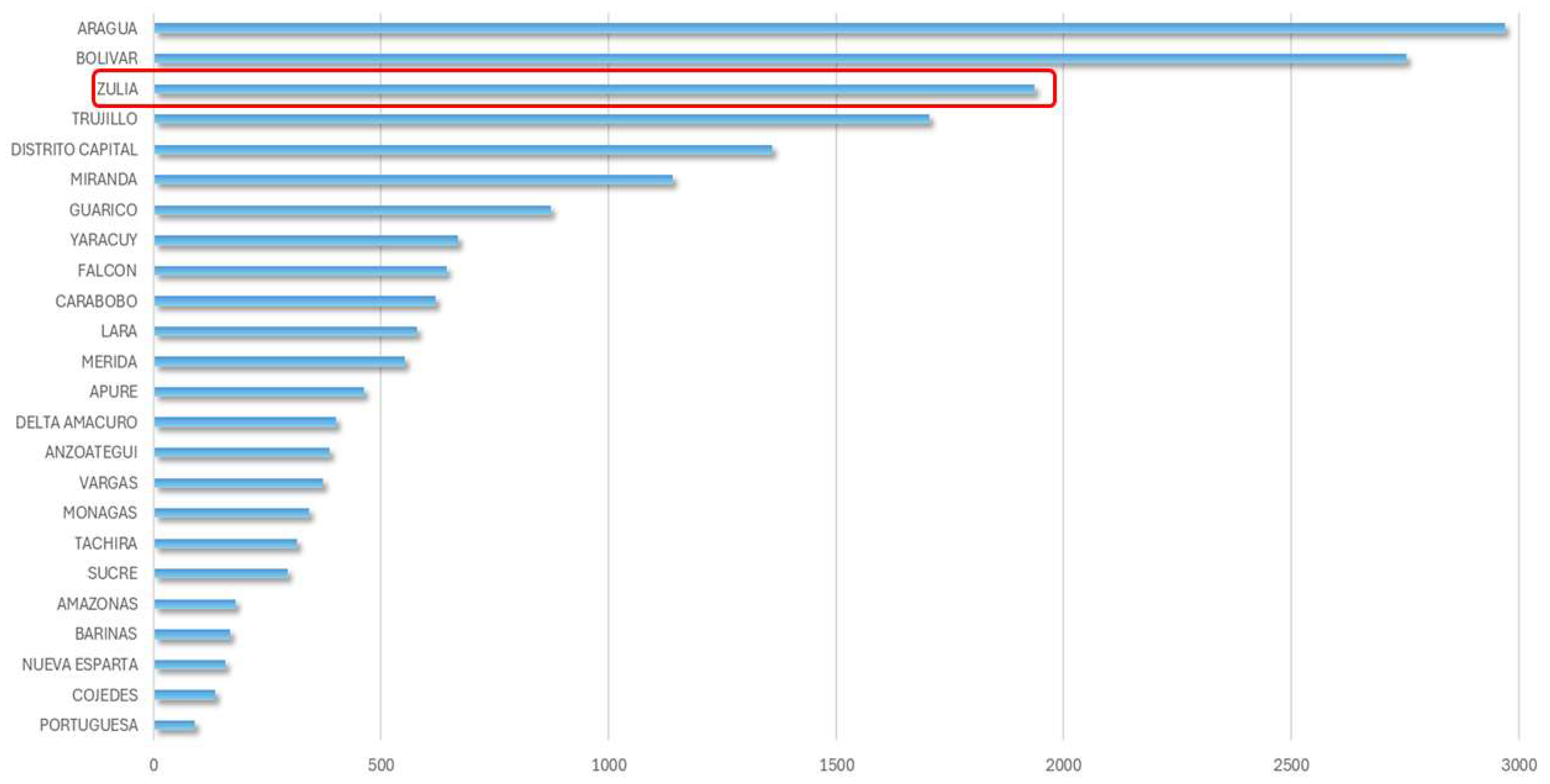
Figure 2.
ML models are most frequently used to conduct studies to predict dengue outbreaks.
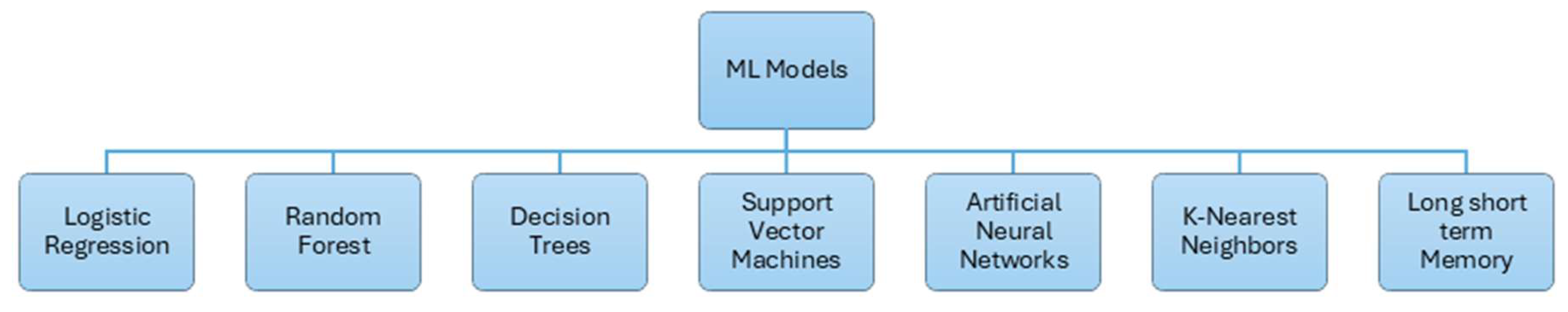
Figure 3.
Zulia State municipalities, Venezuela.
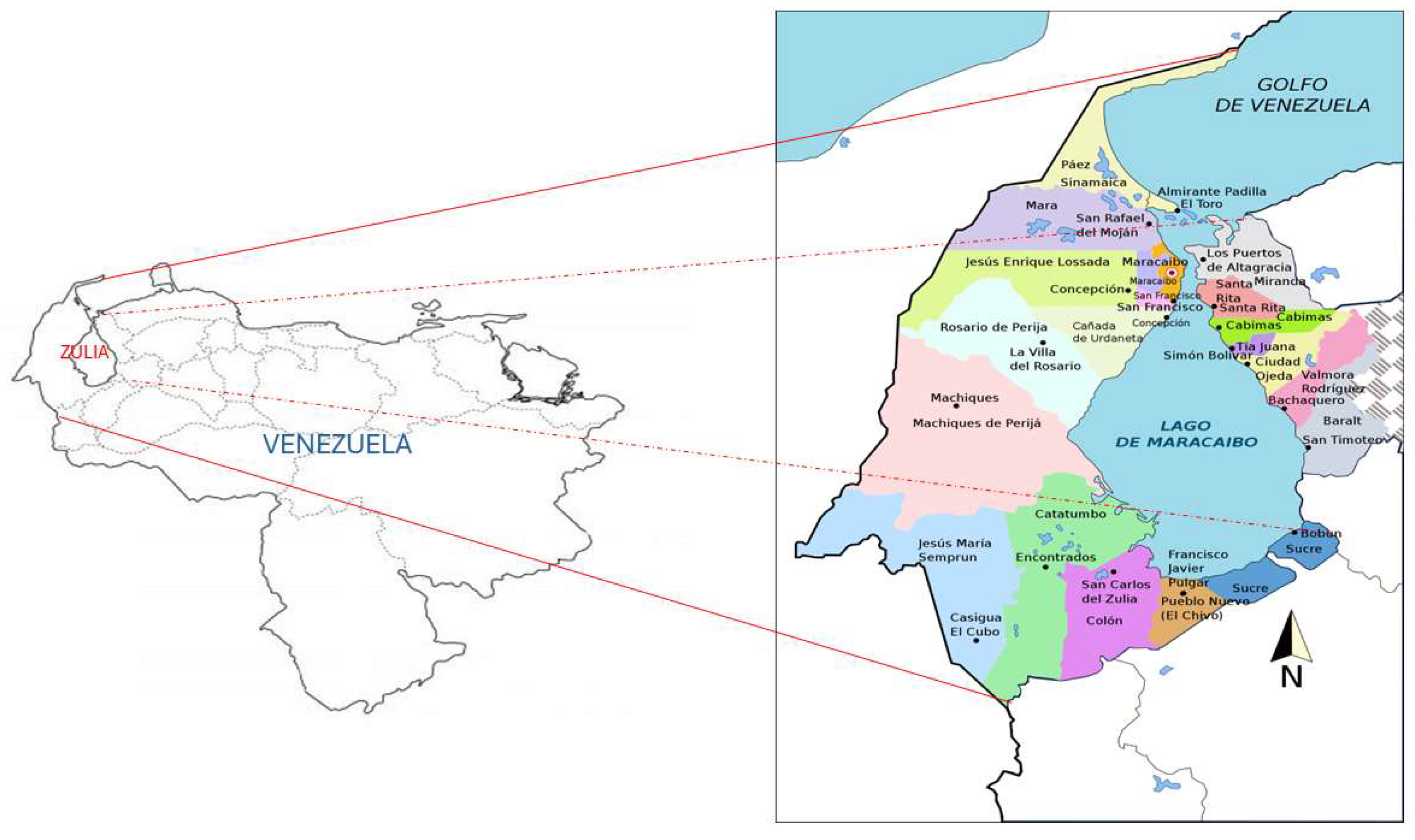
Figure 4.
Data integration.
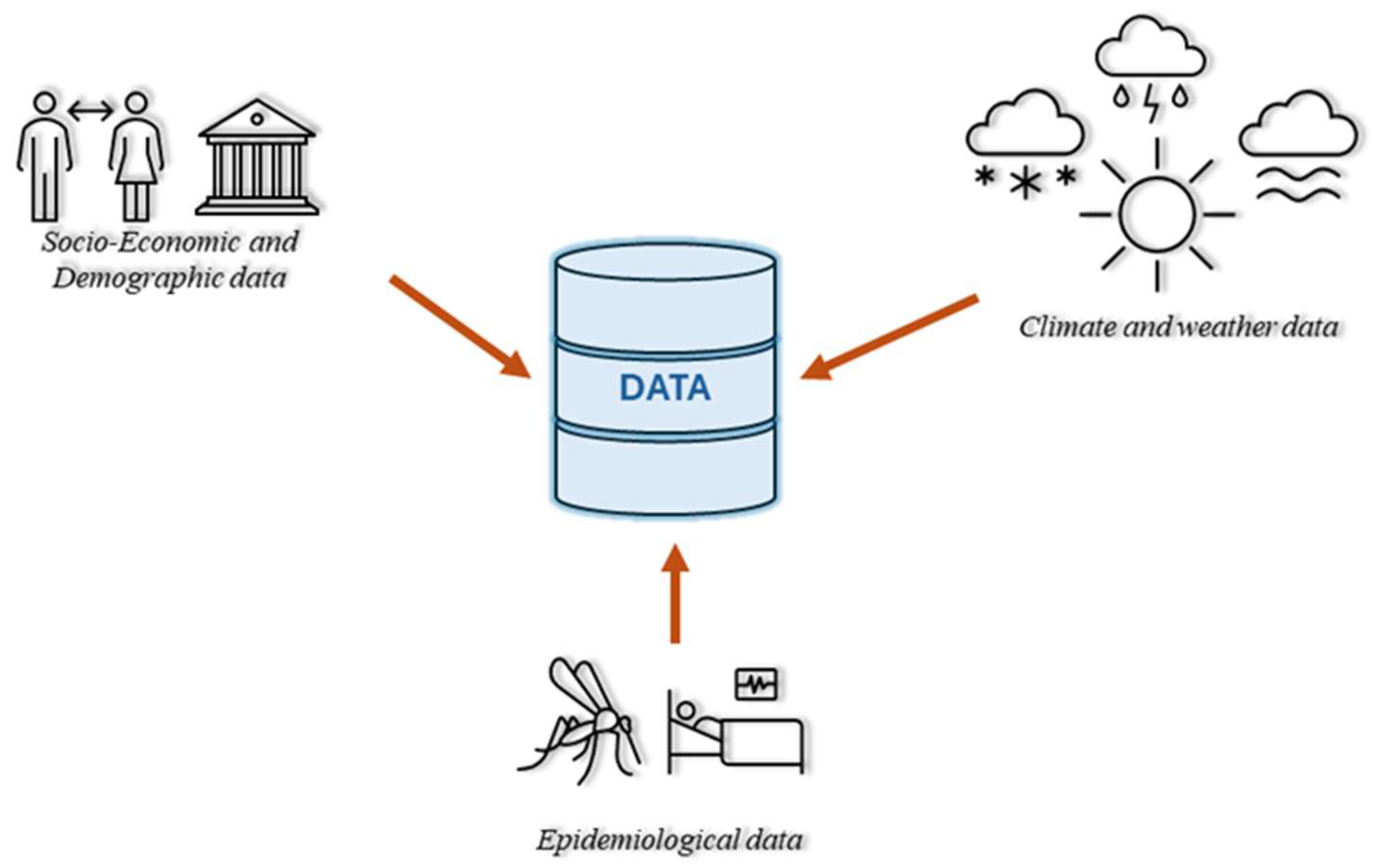
Figure 5.
Experimental processes for constructing a forecast tool for dengue cases in Zulia state, Venezuela based on the traditional kernel machines learning: SVR and Gaussian Processes due to their effectiveness, flexibility and ease of use.
Figure 5.
Experimental processes for constructing a forecast tool for dengue cases in Zulia state, Venezuela based on the traditional kernel machines learning: SVR and Gaussian Processes due to their effectiveness, flexibility and ease of use.
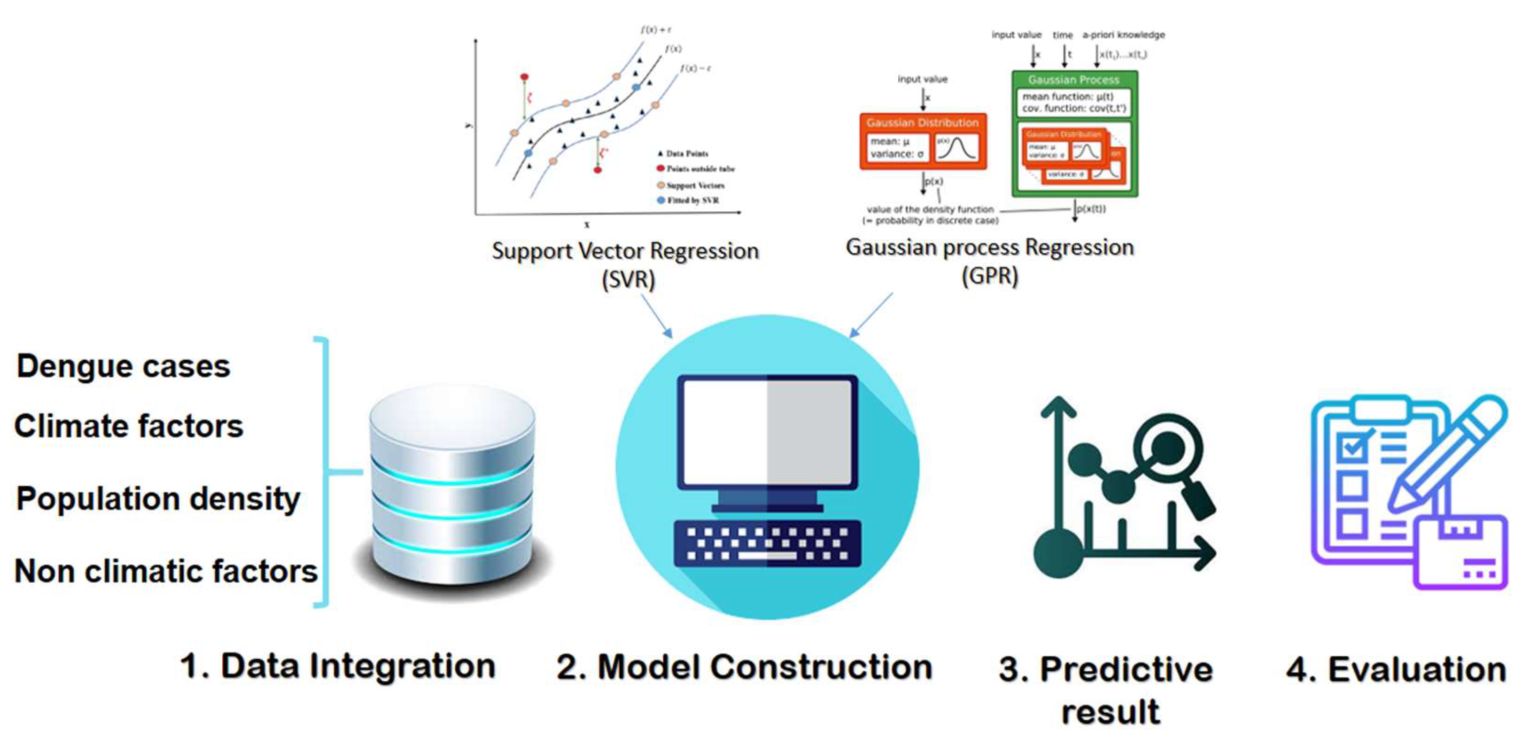
Figure 6.
Results of the GPR prediction along with the actual cases of dengue for certain municipalities with two-week lag in the effect of climate on the incidence of dengue cases.
Figure 6.
Results of the GPR prediction along with the actual cases of dengue for certain municipalities with two-week lag in the effect of climate on the incidence of dengue cases.
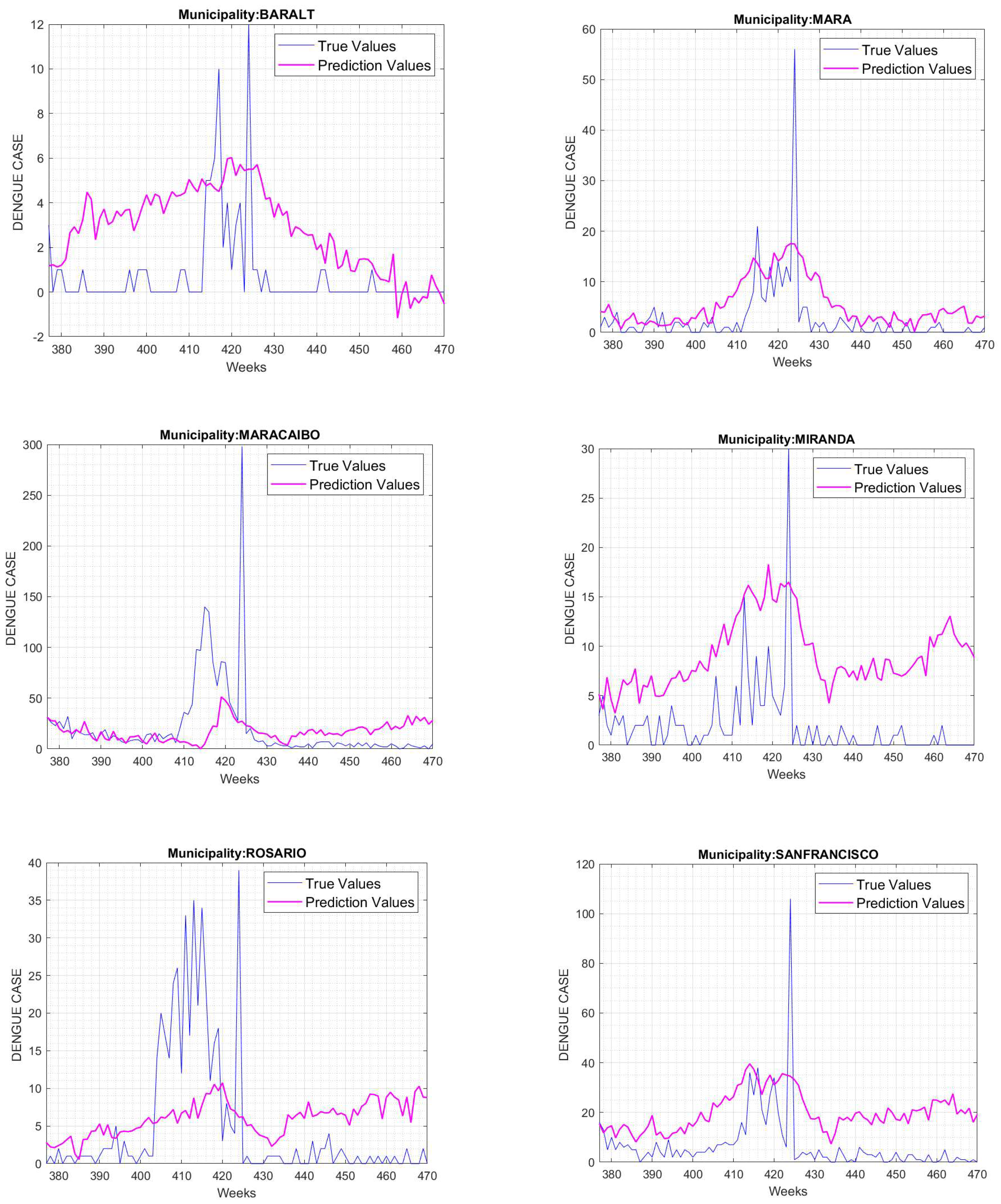
Figure 7.
Results of the SVR prediction along with the actual cases of dengue for certain municipalities.
Figure 7.
Results of the SVR prediction along with the actual cases of dengue for certain municipalities.
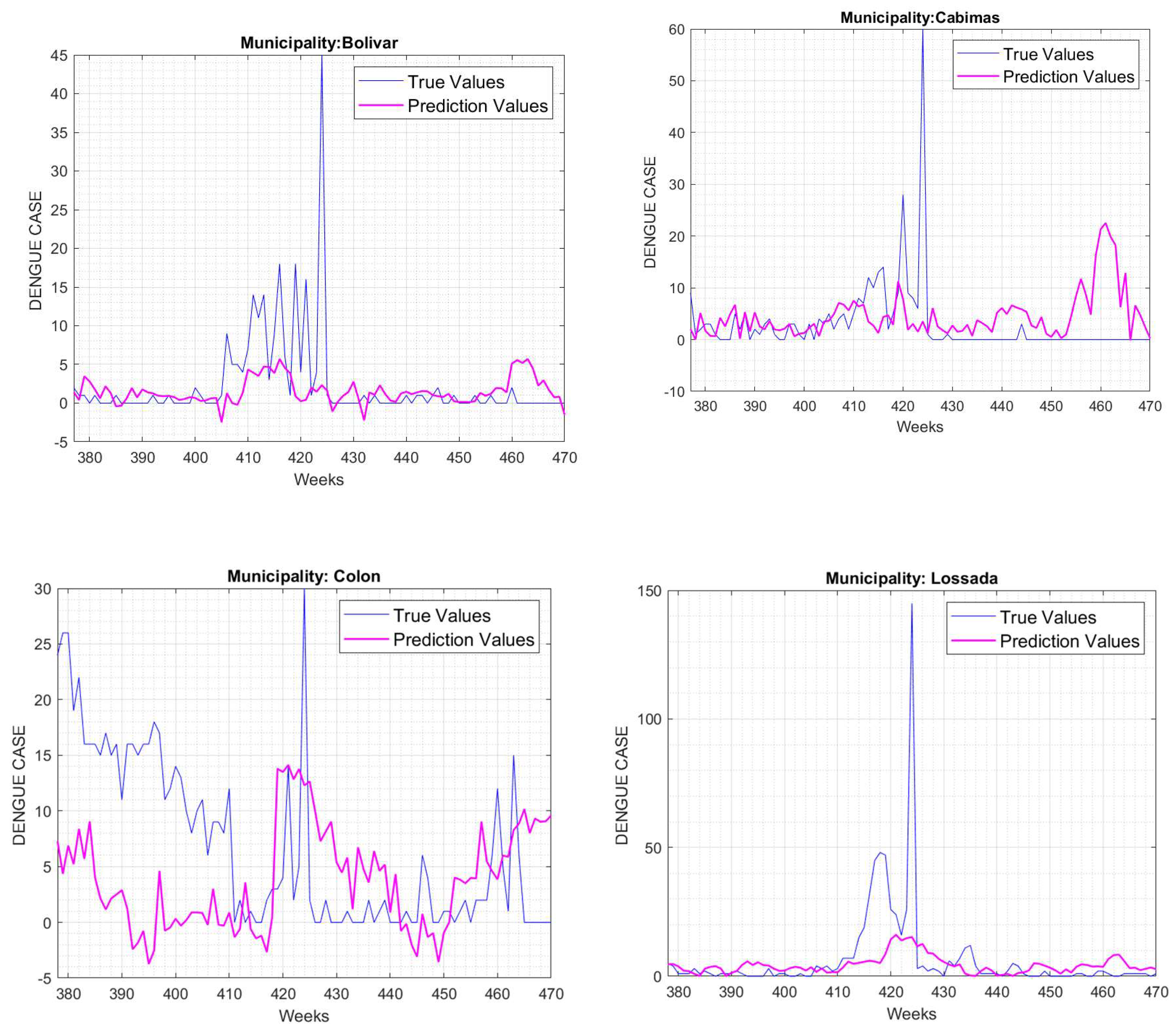
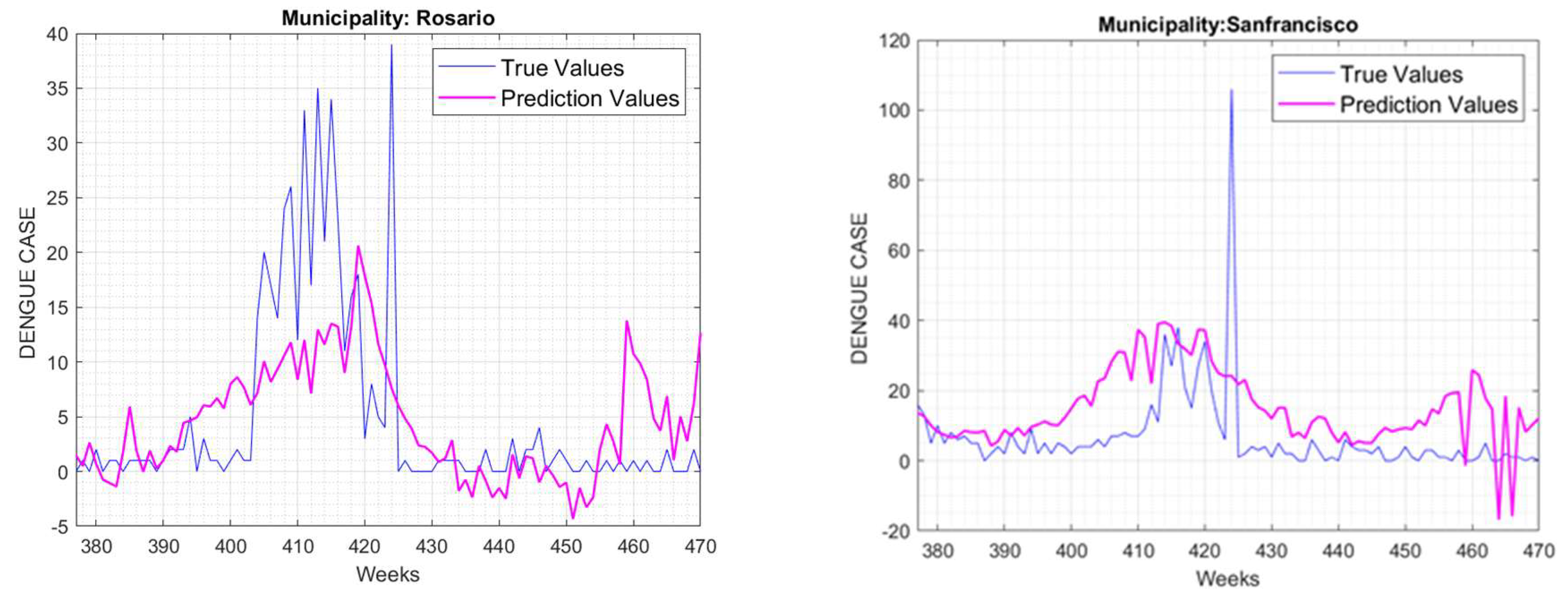

Table 1.
Common kernel functions for SVM-R implementation: (i) The simplest kernel function (linear kernel); (ii) Non-linear classical kernel function (polynomial kernel) and a powerful kernel (radial basis function RBF).
Table 1.
Common kernel functions for SVM-R implementation: (i) The simplest kernel function (linear kernel); (ii) Non-linear classical kernel function (polynomial kernel) and a powerful kernel (radial basis function RBF).
| Kernel | Mathematical Function | Reference |
|---|---|---|
| Linear | (Kesorn, K. et al. 2015) | |
| Polynomial | (Kesorn, K. et al. 2015; Mello-Roman, J., et al. 2019) | |
| Radial basis function (RBF) | (Kesorn, K. et al. 2015; Nordin, N. I. et al., 2020). |
Table 2.
RMSE and lags.
| MUNICIPALITY | Lags | RMSE |
|---|---|---|
| Baralt | 2 | 2.94 |
| Cabimas | 3 | 7.13 |
| Colon | 3 | 6.26 |
| Lossada | 2 | 15.35 |
| Mara | 2 | 5.84 |
| Maracaibo | 2 | 35.36 |
| Miranda | 2 | 8.09 |
| Rosario | 2 | 7.80 |
| San Francisco | 3 | 16.20 |
Table 3.
RMSE and lags using SVR.
| MUNICIPALITY | Lags | RMSE |
|---|---|---|
| Baralt | 2 | 2.57 |
| Cabimas | 2 | 8.14 |
| Colon | 3 | 9.43 |
| Lagunillas | 2 | 2.38 |
| Mara | 2 | 7.005 |
| Lossada | 3 | 16.12 |
| Miranda | 3 | 4.43 |
| Padilla | 2 | 2.16 |
| Rosario | 2 | 7.23 |
| San Francisco | 2 | 15.85 |
Disclaimer/Publisher’s Note: The statements, opinions and data contained in all publications are solely those of the individual author(s) and contributor(s) and not of MDPI and/or the editor(s). MDPI and/or the editor(s) disclaim responsibility for any injury to people or property resulting from any ideas, methods, instructions or products referred to in the content. |
© 2024 by the authors. Licensee MDPI, Basel, Switzerland. This article is an open access article distributed under the terms and conditions of the Creative Commons Attribution (CC BY) license (http://creativecommons.org/licenses/by/4.0/).
Copyright: This open access article is published under a Creative Commons CC BY 4.0 license, which permit the free download, distribution, and reuse, provided that the author and preprint are cited in any reuse.


