Preprint
Article

Near-Exact Analytical Solution of the Sir-Model for the Precise Temporal Dynamics of Epidemics

This version is not peer-reviewed.

Submitted:

06 November 2024

Posted:

07 November 2024

You are already at the latest version

Abstract
A near-exact analytical solution of the statistical Susceptible-Infectious-Recovered (SIR) epidemics model for a constant ratio k0 of infection to recovery rates is derived. The derived solution is not of inverse form as the known solutions in the literature but expresses rather directly the three compartmental fractions S(τ ), I(τ ) and R(τ ) and thus the rate of new infections j(τ ) = S(τ )I(τ ) in terms of the single function U (τ ) and the reduced time τ (the time-integrated infection rate), involving the principal and non-principal branches of Lambert’s function. Exact analytical formulas for the peak time and the maximum fraction of I(τ ) are obtained proving that the rate of new infections peaks before the fraction of infected persons. Our analysis is not entirely analytically exact because the reduced time dependence of the function U (τ ) obeying a nonlinear integro-differential equation is only obtained approximately by expanding a double-exponential function to first-order at small reduced times, and employing an accurate simple approximation of the principal Lambert function at large times, respectively.
Keywords: 
Subject: 
Computer Science and Mathematics  -   Applied Mathematics
Preprints on COVID-19 and SARS-CoV-2

1. Introduction

The Susceptible-Infectious-Recovered (SIR) model is the simplest of the compartmental models used for the mathematical modeling of infectious diseases in order to reproduce or predict the temporal evolution of infectious diseases in human populations. Originally developed nearly hundred years ago [1,2] it lately has become very popular and widespread [3,4,5,6,7,8,9,10,11,12,13,14,15,16,17,18,19,20,21,22,23,24,25,26,27,28,29,30,31,32,33,34,35,36,37,38,39,40,41,42,43] due to its successful applications to the outbreaks of the corona virus in many countries [44]. The considered population of N 1 initially susceptible persons is assigned to the three compartments S ( t ) (susceptible), I ( t ) (infectious), or R ( t ) (recovered/removed). Persons from the population may progress between these compartments described by the time-dependent infection ( a ( t ) and recovery ( μ ( t ) ) rates.
The three respective population fractions obey the sum constraint condition
I ( t ) + S ( t ) + R ( t ) = 1
at any time, and their temporal evolution is given by the SIR-equations
d S ( t ) d t = a ( t ) S ( t ) I ( t ) ,
d I ( t ) d t = a ( t ) S ( t ) I ( t ) μ ( t ) I ( t ) ,
d R ( t ) d t = μ ( t ) I ( t ) .
Besides numerical solutions it is of high interest to derive analytical solutions of the underlying dynamical SIR-equations. In the most general case of a time-dependent ratio k ( t ) = μ ( t ) / a ( t ) between the recovery and the infection rate analytical approximate solutions were derived [45,46] which are very accurate if the cumulative fraction of infections J ( t ) = 1 S ( t ) is small compared to unity at all times.
Recently, new analytical solutions became available [47,48] for an arbitrary time dependence of the infection and recovery rates, provided that the ratio between the two rates is independent of time, for two different types of initial conditions. We refer to these in the following as KSSIR solutions. The utility of the KSSIR solutions were proven by their successful application to past waves of the corona virus [47]. However, in both cases the KSSIR solutions could only be given in inverse form t ( S ) involving an integral, that had to be approximated by second-order polynomials (see [47] for details). Here we consider an alternative approach to the KSSIR solution that avoids the inverse form adopting the semi-time initial conditions [49,50,51,52,53,54,55,56,57,58,59]
S ( 0 ) = 1 η , I ( 0 ) = η , R ( 0 ) = 0 ,
with 0 < η O ( 1 / N ) 1 denoting the initial seed infection fraction of the population.
Two quantities are of particular interest in studies of infections [60,61,62,63,64,65,66,67,68,69,70,71,72,73,74,75,76,77,78,79,80,81,82,83,84,85,86,87,88,89,90,91,92,93,94,95,96,97,98,99,100,101]:
(1)
the differential rate of newly infected persons from the desease
J ˙ ( t ) = a ( t ) I ( t ) S ( t ) ,
which, with a delay time t d of about a week, determines the death rate d ( t ) = f N j ( t t d ) , where the mortality rate f is of the order 10 2 10 3 varying for different mutants of the Covid virus and different countries [102]. J ˙ ( t ) also determines the hospitalization rate of seriously infected persons.
(2)
the fraction of infected persons I ( t ) determines the peak time of required clinical resources in the host country of the considered population [103].
Both quantities J ˙ ( t ) and I ( t ) first increase in time, undergo a maximum and drop at late times. While exact analytical formulas for the peak time τ j and the peak rate of new infections J ˙ max are available in the KSSIR-model, several different approximations for the peak time τ j and the peak fraction of infected persons I max have been derived [103]. It is one purpose of the present study to derive exact expressions for τ I and I max .

2. Reduction of the General SIR-Equations

By introducing the reduced time
τ = t 0 t d ξ a ( ξ )
for arbitrary but given real time dependent infection rates a ( t ) and the ratio
k ( τ ( t ) ) = μ ( t ) a ( t )
the SIR-equations (1)-(3) can be written as
d S ( τ ) d τ = S ( τ ) I ( τ ) ,
d I ( τ ) d τ = S ( τ ) I ( τ ) k ( τ ) I ( t ) ,
d R ( τ ) d τ = k ( τ ) I ( τ ) ,
1 = S ( τ ) + I ( τ ) + R ( τ ) ,
subject to initial conditions
S ( τ = 0 ) = 1 η , I ( τ = 0 ) = η , R ( τ = 0 ) = 0 .
From the invariant J ˙ ( t ) d t = j ( τ ) d τ we obtain with Equation (5) in the form d τ / d t = a ( t ) for the differential rate of newly infected persons from the desease
j ( τ ) = d J ( τ ) d τ = J ˙ ( t ) a ( t ) = S ( τ ) I ( τ ) = d S ( τ ) d τ
with the initial value j ( 0 ) = η ( 1 η ) . The invariant ( J ( t ) = J ( τ ) ) cumulative distribution corresponding to j ( τ ) is given by
J ( τ ) = τ d τ j ( τ ) = J ( 0 ) 0 τ d τ d S ( τ ) d τ = J ( 0 ) + S ( 0 ) S ( τ ) = 1 S ( τ ) ,
where the initial condition J ( 0 ) = I ( 0 ) = η had been used, in accord with Equation (8).

2.1. Reduction

Equation (7a) readily yields
I ( τ ) = d ln S ( τ ) d τ = d S ( τ ) / d τ S ( τ ) ,
whereas Equation (7b) provides
d ln I ( τ ) d τ = S ( τ ) k ( τ ) ,
which with the initial condition on I ( 0 ) = η integrates to
I ( τ ) = η e U ( τ ) ,
U ( τ ) = 0 τ d x [ S ( x ) k ( x ) ] .
Combining Equations (11) and (13) with
S ( τ ) = d U ( τ ) d τ + k ( τ )
then leads to the single nonlinear differential equation
d d τ ln d U ( τ ) d τ + k ( τ ) = η e U ( τ )
for U ( τ ) . Equation (16) integrates to
d U ( τ ) d τ + k ( τ ) = ( 1 η ) exp η 0 τ d x e U ( x ) ,
where we made use of the initial condition S ( 0 ) = 1 η .

2.2. Stationary Ratio

Throughout this study a stationary ratio (6) is assumed, i.e.,
k ( τ ) = k 0 = const .
k 0 often is referred to as inverse reproduction number. The derived exact analytical solutions then hold for stationary infection and recovery rates as well as for any time-dependent infection rate a ( t ) provided the recovery rate μ ( t ) a ( t ) has the same time variation while its absolute value can be different.
For a stationary ratio Equations (14) and (16)–(17) simplify to
U ( τ ) = 0 τ d x S ( x ) k 0 τ ,
d d τ ln d U ( τ ) d τ + k 0 = η e U ( τ ) ,
d U ( τ ) d τ + k 0 = ( 1 η ) e η 0 τ d x e U ( x ) ,
d 2 U ( τ ) d τ 2 = η ( 1 η ) U ( τ ) e η 0 τ d x e U ( x ) .
In earlier work [48] Equations (7) were solved exactly in inverse form as
τ = η J d x ( 1 x ) x + k 0 ln 1 x 1 η ,
allowing important conclusions on the final values of the fractions S , I , R (see Appendix A for details). Here we will follow a different approach avoiding the necessary inversion of solution (20) to derive J ( τ ) . However, the noted exact results from Appendix A will be used below to check the validity of the alternative solution.

3. Exact Solution

3.1. Ansatz

The ansatz
d U ( τ ) d τ + k 0 = k 0 W a e b e U ( τ )
in terms of the Lambert [104] function W ( Z ) (see Appendix G of ref. [105]) and yet unspecified constants a and b provides for Equation (19c)
k 0 W ( a e b e U ( τ ) ) = ( 1 η ) e η 0 τ d x e U ( x ) .
Note that the ansatz (21) is equivalent to
k 0 τ = U d x 1 + W ( a e b e x ) .
Next, we will determine the constants a and b and thus prove that the ansatz (21) fulfills the differential equation (19c). Applying the defining equation for the Lambert function
W ( Z ) = Z e W ( Z )
yields for Equation (22)
η 0 τ d x e U ( x ) = W a e b U ( τ ) b e U ( τ ) ln k 0 a 1 η .
Hence for its derivative with respect to τ , with
Z ( τ ) = a e b e U ( τ ) ,
one obtains
η e U ( τ ) = d U d τ d d U W ( a e b e U ) b e U = d U d τ d Z d U d d Z W ( Z ) b e U   = d U d τ b e U Z d d Z W ( Z ) b e U = d U d τ b e U Z d d Z W ( Z ) 1   = d U d τ b e U W ( Z ) 1 + W ( Z ) 1 = d U d τ b e U ( τ ) 1 + W ( Z ) ,
where we used the differential equation
Z d W ( Z ) d Z = W ( Z ) 1 + W ( Z )
for Lambert functions. The Equation (28) can be written as
d τ d U = b / η 1 + W ( Z ) ,
which is solved by
τ = b η U d x 1 + W ( a e b e x ) .
In order for the solution (30) to be consistent with Equation (23) one has to demand that b = η / k 0 . Consequently, the exact solution is given by
k 0 τ = U d x 1 + W a e η e x k 0 ,
where we still have to determine the constant a and the lower integration limit from the initial condition and we have to identify the appropriate branch of the Lambert function.
If we re-use U ( 0 ) = 0 and U ( 0 ) = 1 η k 0 , then we can determine a from Equation (27) evaluated at τ = 0 ,
1 = 1 η k 0 k 0 [ 1 + W ( a e η / k 0 ) ] ,
or equivalently
W ( a e η / k 0 ) = 1 η k 0 .
With Equation (24) written as
Z = W e W ,
Equation (33) can be solved for a and provides
a = ( 1 η ) e 1 / k 0 k 0 = α ,
with α from Equation (A9) in Appendix A.
To conclude, Equation (21) is formally solved by
τ = 1 k 0 U d x 1 + W 1 η k 0 e ( 1 η e x ) / k 0 = 1 k 0 U d x 1 + W α e η e x k 0 ,
but we have to make this more precise, as the Lambert function W has two branches, W 0 and W 1 .
For positive k 0 and η [ 0 , 1 ) the argument of the Lambert function is negative because α < 0 . Recall that W ( Z ) = 1 for Z = 1 / e , where the two Lambert branches meet. Let τ U and U max denote the peak time and peak amplitude of U ( τ ) . The peak amplitude U max = U ( τ U ) is determined by the solution of Z = 1 / e , and thus given by
U max = ln 1 + ln ( a ) b = ln 1 k 0 k 0 ln 1 η k 0 η .
For times up to peak time the solution (36) applies, using the non-principal branch of Lambert’s function,
τ = 1 k 0 0 U d x 1 + W 1 α e η e x k 0 ( 0 τ τ U ) ,
with the peak time τ U determined by
τ U = 1 k 0 0 U max d x 1 + W 1 α e η e x k 0 .
Over this interval U ( τ ) monotonically increases from U ( 0 ) = 0 to U ( τ U ) = U max . Beyond peak time, the solution is determined by
τ = τ U + 1 k 0 U U max d x 1 + W 0 α e η e x k 0 ( τ τ U ) .
Over this remaining interval U ( τ ) monotonically decreases towards lim τ U ( τ ) = .
The respective slopes below and above the peak time are obtained by taking the derivative with respect to τ of Equations (38) and (40) providing
d U d τ ( τ τ U ) = k 0 1 + W 1 α e η e U ( τ ) k 0
and
d U d τ ( τ τ U ) = k 0 1 + W 0 α e η e U ( τ ) k 0 ,
respectively. At very large times the latter approaches
lim τ d U d τ = k 0 [ 1 + W 0 ( α ) ] ,
since lim τ U ( τ ) = .

3.2. Resulting Fractions

Using the notation W s ( Z ) and W s ( Z ) = d W s ( Z ) / d Z with s = 1 for τ τ U and s = 0 for τ τ U , respectively, and
Z = 1 η k 0 e η e U ( τ ) 1 k 0 = α e η e U ( τ ) k 0 = exp η k 0 e U ( τ ) e U max 1 ,
with negative α , the solutions Equations (41)–(42) read
d U d τ = k 0 [ 1 + W s ( Z ) ] .
Then, according to Equation (15) one finds
S ( τ ) = U ( τ ) + k 0 = k 0 W s ( Z ) = k 0 W s α e η e U ( τ ) k 0 ,
so that with Z = α
S = S ( τ = ) = k 0 W 0 ( α ) ,
in agreement with the exact KSSIR result (A10a). Using
d Z d τ = η k 0 d U ( τ ) d τ e U ( τ ) Z = η Z e U ( τ ) 1 + W s ( Z ) ,
one obtains for the first derivative of Equation (46) with respect to τ
d S d τ = k 0 d Z d τ W s ( Z ) = η k 0 Z e U ( τ ) [ 1 + W s ( Z ) ] W s ( Z ) = η k 0 e U ( τ ) W s ( Z ) ,
where we used Lambert’s equation (28). Inserting Equations (46) and (49) yields for Equation (11)
I ( τ ) = d S ( τ ) / d τ S ( τ ) = η e U ( τ ) = d d τ ln U ( τ ) + k 0 = U ( τ ) U ( τ ) + k 0 ,
where we used Equation (19b), thus correctly reproducing the earlier Equation (13). Obviously, the fraction of infected persons peaks at τ U , because of its dependence e U ( τ ) , and its maximum value is given by
I max = η e U max = 1 k 0 k 0 ln 1 η k 0
Consequently, one finds for the rate of new infections (9)
j ( τ ) = S ( τ ) I ( τ ) = U ( τ ) = η ( 1 η ) U ( τ ) e η 0 τ d x e U ( x ) ,
where in the last step we used Equation (19d), and the corresponding cumulative fraction of infected persons
J ( τ ) = 1 S ( τ ) = 1 + k 0 W s ( Z ) = 1 + k 0 W s α e η e U ( τ ) k 0 .
Likewise, the sum constraint (7d) leads to
R ( τ ) = 1 S ( τ ) j ( τ ) 1 J ( τ ) = 1 k 0 U ( τ ) + U ( τ ) U ( τ ) + k 0
As U ( ) = we derive
I = j = 0 ,
R = J = 1 S = 1 + k 0 W 0 ( α ) ,
reproducing exactly the earlier noted properties (A8) and (A10).
We thus have expressed all quantities of interest, the fractions S , I , R as well as the differential rate of new infections and its corresponding cumulative number in terms of the function U ( τ ) and its first and second derivatives. These expressions are exact. It remains to derive the direct reduced time dependence of the function U ( τ ) which is done approximately for large and small times in the following sections.

4. Approximated U ( τ ) for Large and Small Times

4.1. Large Times τ τ U

We note that the function Z ( τ ) in Equation (44) has values
Z ( τ U ) = e 1 , Z ( τ = ) = α = ( 1 η ) e 1 k 0 k 0 ,
so that 0 < | Z ( τ = ) | < | Z ( τ U ) | < e 1 . For such small values of Z we then use as approximation
W 0 ( Z ) ( 1 + e Z ) 1 / 2 1 ,
shown in Figure 1 in comparison to the exact variation. As can be seen the agreement is sufficient, and the approximation exact at the terminals.
The approximation (57) then yields for Equation (40)
k 0 ( τ τ U ) U U max d x 1 + α e exp ( η e x / k 0 ) = η e U k 0 η e U max k 0 d y y 1 + α e e y ,
where we substituted y = η e x / k 0 . The upper integration limit is given by
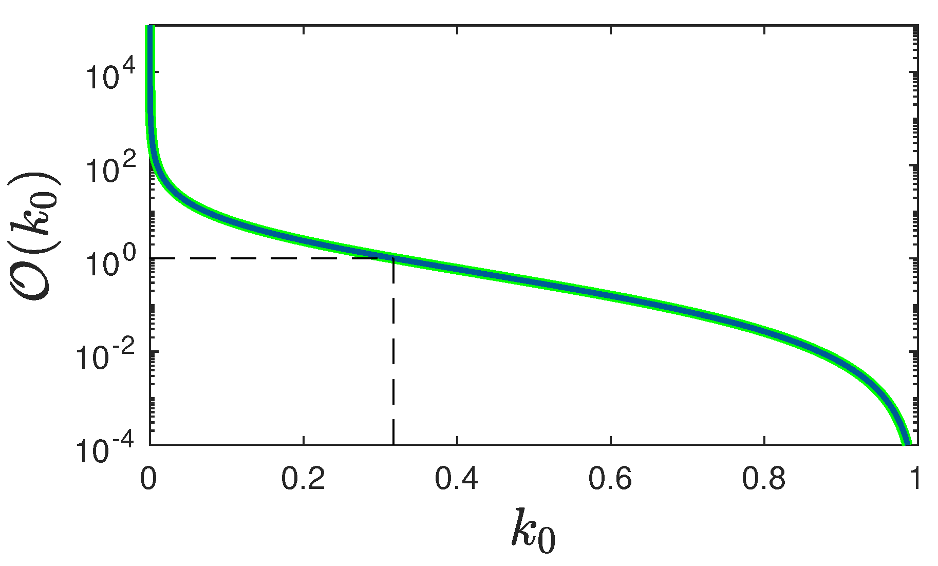
O ( k 0 ) = η e U max k 0 = 1 k 0 1 + ln 1 η k 0 1 k 0 + ln ( k 0 ) 1 ,
where the second approximation holds for small values of η 1 . It is shown in Figure 2 as a function of k 0 . The upper integration limit is thus smaller than unity provided k 0 ( 2 ln k 0 ) > 1 , corresponding to
k 0 > W 1 ( e 2 ) 0.32
in agreement with Figure 2.
For such values of k 0 we approximate
1 + α e e y 1 + α e + α e y
to obtain with
κ = α e 1 + α e = k 0 1 η e 1 k 0 1 1 1 = e η e U max k 0 1 1 = 1 e O ( k 0 ) 1
for the integral (58)
1 + α e k 0 ( τ τ U ) = k 0 ( τ τ U ) 1 + κ η e U k 0 η e U max k 0 d y y 1 κ y
With the substitution s = 1 κ y one finds for the last equation
k 0 ( τ τ U ) 1 + κ = 1 η κ e U max k 0 1 η κ k 0 e U d s ( 1 s ) s = 2 tanh 1 s 1 η κ e U max k 0 1 η κ k 0 e U     = ln 1 + s 1 s 1 η κ e U max k 0 1 η κ k 0 e U
After straightforward algebra Equation (64) leads to
η κ e U ( τ ) k 0 = 1 tanh 2 k 0 ( τ τ U ) 2 1 + κ + Φ = cosh 2 k 0 ( τ τ U ) 2 1 + κ + Φ
with the constant Φ defined by
Φ = 1 2 ln 1 + 1 η κ e U max k 0 1 1 η κ e U max k 0 = tanh 1 1 κ η k 0 e U max
Equation (65) readily provides as approximation at large times
U ( τ τ U ) = U H ( τ ) = ln k 0 η κ 2 ln cosh ζ ( τ ) ,
ζ ( τ ) = k 0 ( τ τ U ) 2 1 + κ + Φ .
We note that Equation (67) correctly provides U H ( τ U ) = U max as cosh ( ζ ( τ U ) ) = cosh Φ = k 0 / η κ e U max .
The slope of the approximation (67) is
U ( τ τ U ) = k 0 1 + κ tanh ζ ( τ ) ,
providing for its limiting slope
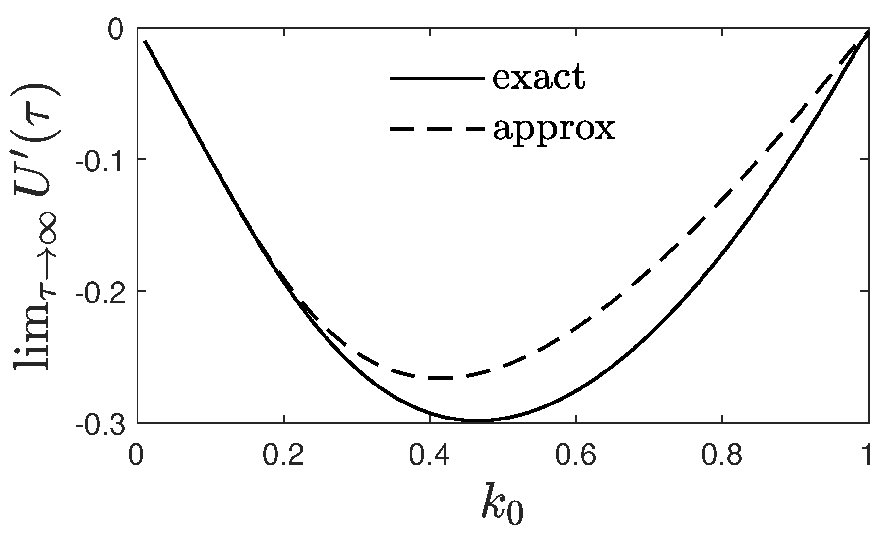
lim τ d U H d τ = k 0 1 + κ = k 0 k 0 ( 1 η ) e 1 1 k 0 ,
which Figure 3 compares favorably well with the exact limiting slope given by Equation (43).
It is tempting to use approximation (67) to calculate the corresponding U ( τ τ U ) as in Equation (69) and U ( τ τ U ) to infer directly the three fractions S, I and R as well as the differential rate j at large times. However, this produces incorrect results as can be seen with the resulting
S ( τ τ U ) = U ( τ τ U ) + k 0 = k 0 [ 1 tanh ζ ( τ ) 1 + κ ]
implying
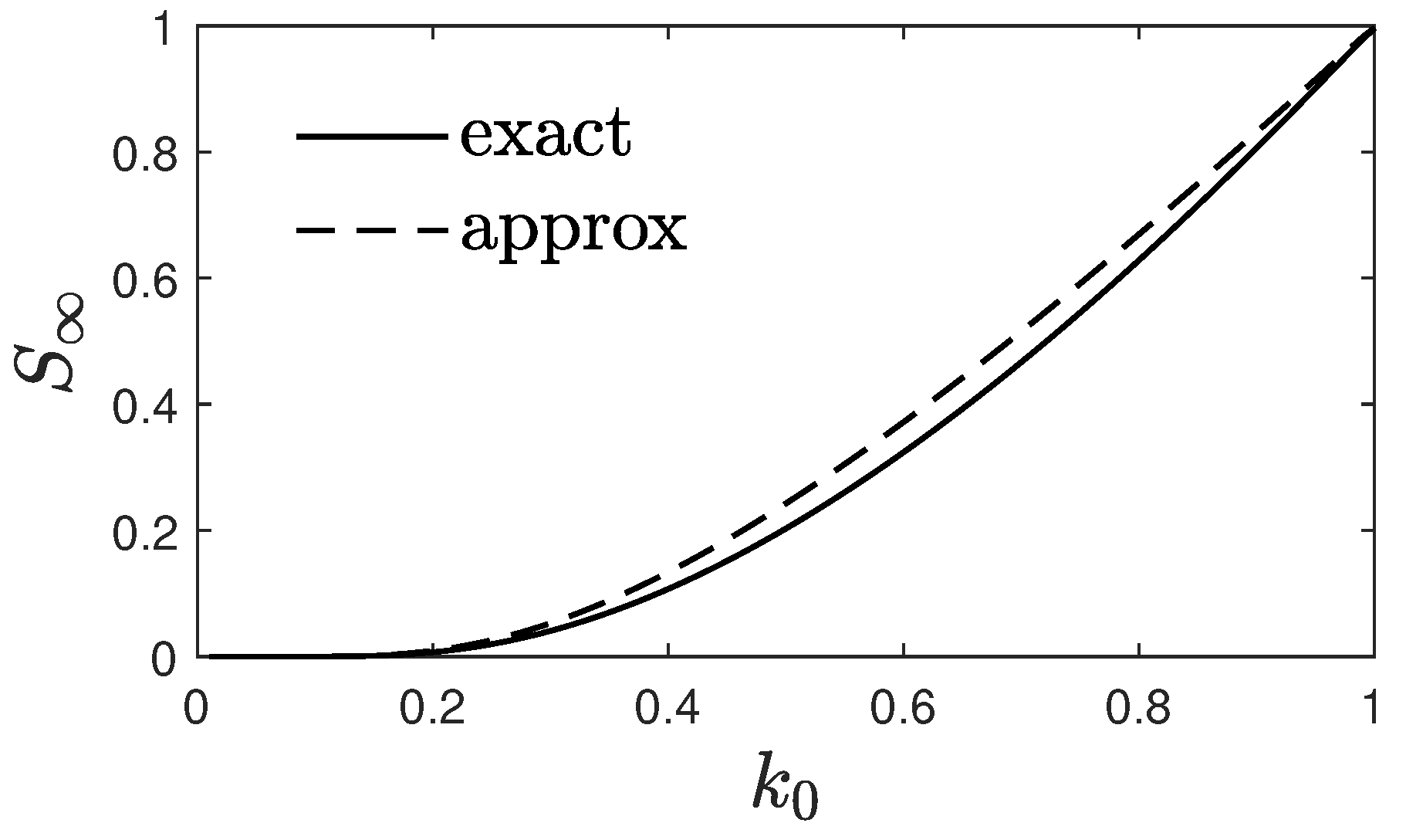
S = k 0 1 1 1 + κ = k 0 1 1 1 η k 0 e 1 1 k 0 1 η 2 k 0 e 1 1 k 0
which is finite but slightly disagrees with the exact final value (47), as shown in Figure 4.
The proper way to continue is to only use Equation (67) as an approximation for U ( τ τ U ) and to insert it in the earlier general expressions for the fractions. With this approximation we obtain for Equation (44)
Z ( τ τ U ) = α exp 1 κ cosh 2 ζ ( τ ) ,
Z ( τ U ) = α exp η e U max k 0 = 1 e ,
and consequently for the fraction (46)
S ( τ τ U ) = 1 J ( τ τ U ) = k 0 W 0 ( Z ( τ τ U ) )   = k 0 W 0 α exp 1 κ cosh 2 ζ ( τ ) ,
which in contrast to the incorrect Equation (72) now correctly approaches S = k 0 W 0 ( α ) . For later use we note
S ( τ U ) = k 0 W 0 ( e 1 ) = k 0
Likewise, the fraction (50) at large times is given by
I ( τ τ U ) = k 0 ln Z α = k 0 κ cosh 2 ζ ( τ ) ,
reproducing correctly I = 0 . The rate of new infections (9) then is
j ( τ τ U ) = S ( τ τ U ) I ( τ τ U ) = k 0 2 W 0 α exp 1 κ cosh 2 ζ ( τ ) κ cosh 2 ζ ( τ )   = k 0 2 W 0 ( Z ) ln Z α .

4.2. Small Times τ τ U

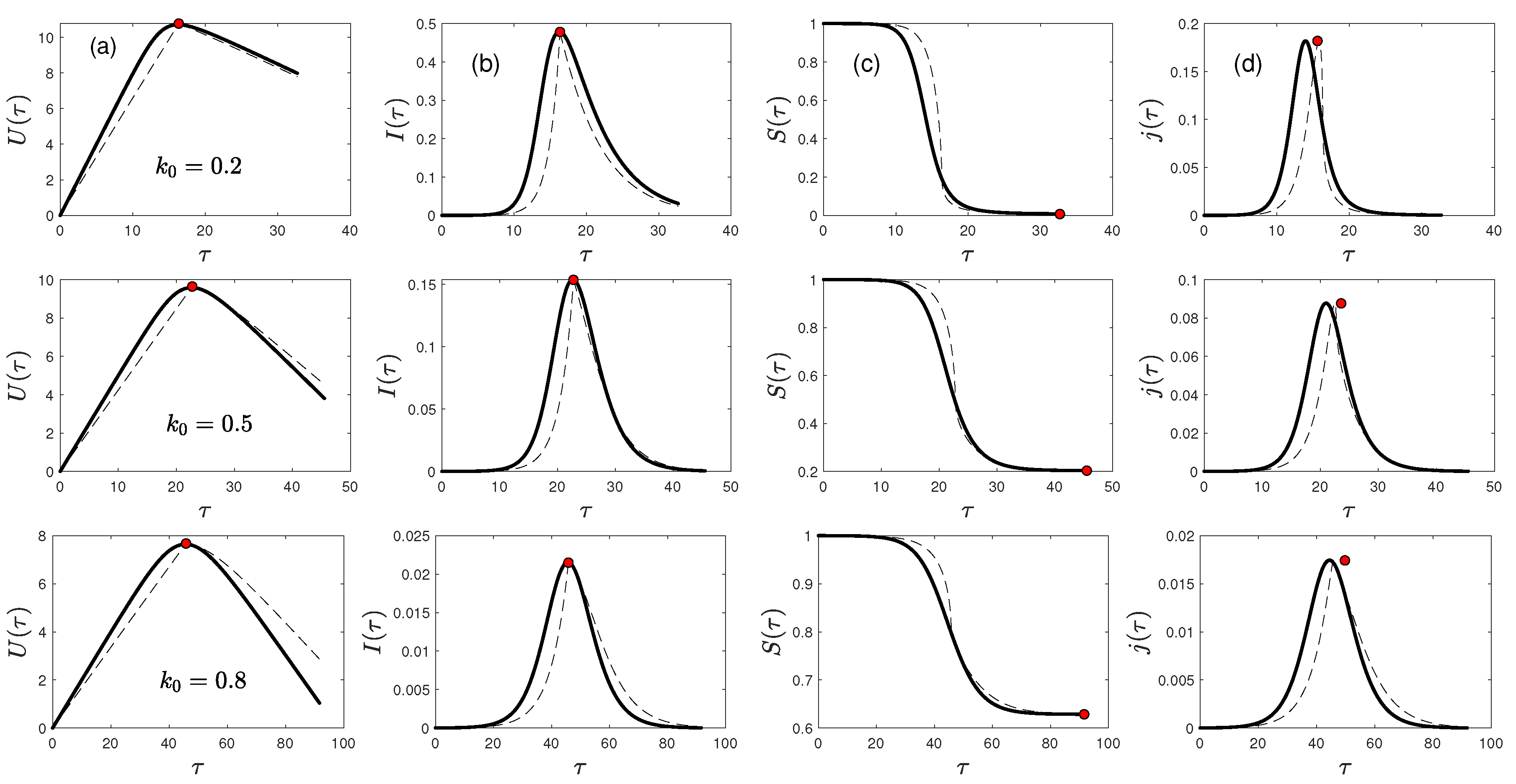
Figure 5. Time evolution of the functions U ( τ ) , I ( τ ) , S ( τ ) , and j ( τ ) . (a) Numerical U ( τ ) from (14) (solid) compared with U ( τ ) from (67) and (85) (dashed), using ζ from Equation (68), Φ from Equation (66), ρ from (82), κ from (62), τ U from (39), U max from (37). The red bullet marks ( τ U , U max ) . (b) Numerical I ( τ ) (solid) compared with I ( τ ) from Equations (76) and (88). The red bullet marks ( τ I = τ U , I max ) from Equations (39) and (51). (c) Numerical S ( τ ) (solid) compared with S ( τ ) from Equations (87) and (74). The red bullet marks S (47). (d) Numerical j ( τ ) (solid) compared with j ( τ ) from Equations (93) with Z s according to Equation (94). The red filled bullet marks ( τ j , j max ) according to Equations (103) and (106). Parameters: η = 10 5 and k 0 { 0.2 , 0.5 , 0.8 } mentioned in the left panel.
Preprints 138757 g005
For small times where U ( τ ) 1 we expand the double-exponential function on the right-hand side of Equation (19c) to first order as
e η 0 τ d x e U ( x ) 1 η 0 τ d x e U ( x ) 1 η 0 τ d x [ 1 + U ( x ) ] = 1 η τ η 0 τ d x U ( x ) ,
so that Equation (19c) becomes
d U ( τ ) d τ + η ( 1 η ) τ + 0 τ d x U ( x ) 1 η k 0 ,
fulfilling the correct initial condition U ( 0 ) = 1 η k 0 . Setting
0 τ d x U ( x ) = F ( τ ) τ + 1 η k 0 η ( 1 η ) ,
Equation (79) reduces to
d 2 F ( τ ) d τ 2 + η ( 1 η ) F ( τ ) = 0 ,
with the solution
F ( τ ) = C 1 sin ( ρ τ ) + C 2 cos ( ρ τ ) , ρ = η ( 1 η ) .
Therefore
0 τ d x U ( x ) = C 1 sin ( ρ τ ) + C 2 cos ( ρ τ ) τ + 1 η k 0 η ( 1 η ) , U ( τ ) = ρ [ C 1 cos ( ρ τ ) C 2 sin ( ρ τ ) ] 1 .
The two integration constants C 1 and C 2 are determined by the conditions U ( 0 ) = 0 and U ( τ U ) = U max yielding
C 1 = 1 ρ , C 2 = cos ( ρ τ U ) 1 U max ρ sin ( ρ τ U ) .
Consequently
U ( τ τ U ) = U L ( τ ) = g ( τ ) 1 ,
g ( τ ) = sin ρ ( τ U τ ) + ( 1 + U max ) sin ( ρ τ ) sin ( ρ τ U ) .
Since U ( τ U ) = U max guarantees, according to Equations (44) and (46), that Z ( τ U ) = e 1 implying W 1 ( Z ( τ U ) ) = 1 , with the approximation (85) also S ( τ U ) = k 0 is in agreement with Equation (75).
For general small times Equation (44) subjected to the approximation Equation (85a) provides
Z ( τ τ U ) = α e η k 0 e g ( τ ) 1 ,
so that Equation (46) leads to
S ( τ τ U ) = 1 J ( τ τ U ) = k 0 W 1 α e η k 0 e g ( τ ) 1 .
Likewise, the fraction (50) at small times is given by
I ( τ τ U ) = η e g ( τ ) 1 ,
reproducing correctly I ( τ = 0 ) = η . The rate of new infections (9) then is
j ( τ τ U ) = S ( τ τ U ) I ( τ τ U ) = η k 0 e g ( τ ) 1 W 1 α e η k 0 e g ( τ ) 1 .
We recall that Equation (39) determines
τ U = 1 k 0 0 U max d x 1 + W 1 α e η e x k 0 .
so that for given values η and k 0 all parameters are fixed.
In most applications the initial fraction of infected persons η O ( 10 5 ) is very small. Hence for reduced times τ τ U η 1 / 2 one can further approximate
sin ( ρ τ ) ρ τ , sin ( ρ τ U ) ρ τ U , sin [ ρ ( τ U τ ) ] ρ ( τ U τ )
to obtain for the function (85b)
g ( τ τ U ) 1 + τ τ U U max ,
i.e., one may replace g ( τ ) 1 in Equations (86)–(89) by τ U max / τ U with U max from Equation (37).

5. Results

5.1. Rate of New Infections

According to Equations (77) and (89) with our earlier notation the rate of new infections at all reduced times is given by
j ( τ ) = k 0 2 W s ( Z s ) ln Z s α
with
Z 1 = Z L = α e η k 0 e g ( τ ) 1 , τ τ U
Z 0 = Z H = α e κ 1 cosh 2 ζ ( τ ) , τ τ U
We note that
Z L α [ e η k 0 , e O ( k 0 ) ] 1 ,
Z H α [ 1 , e O ( k 0 ) ] > 1 .
In the last column of Figure 5 we compare this rate of new infections based on τ U from Equation (90) with the exact numerical solution for η = 10 5 and several choices of the parameter k 0 = 0.2 , 0.5 , 0.8 . One notices excellent agreement between the analytical and numerical curves in all three cases.
Figure 6. Extremum of Z ( τ ) . Z E / α (102) versus (a) e α and (b) k 0 . Shown are the cases of s = 1 (solid) and s = 0 (dashed). For this plot η = 10 5 , but the plots are basically unaffected by η for η 1 .
Preprints 138757 g006
The rate of new infections (93) attains its maximum for a vanishing first derivative
d j ( τ ) d τ = k 0 2 d Z s d τ d d Z s [ W s ( Z s ) ln Z s α ]   = η k 0 2 Z s e U s [ 1 + W s ( Z s ] W s ( Z s ) ln Z s α + W s ( Z s ) Z s   = η k 0 2 e U s W s ( Z s ) [ 1 + W s ( Z s ) ] 1 + Z s W s ( Z s ) W 0 ( Z s ) ln Z s α   = η k 0 2 e U s W s ( Z s ) 1 + W s ( Z s ) + ln Z s α = 0 ,
where we used Equations (48) and (28). Thus the maximum occurs at Z E given by the solution of
1 + W s ( Z E ) + ln Z E α = 0 .
Taking the exponential of the last equation leads to
α e = Z E e W s ( Z E ) = W s ( Z E ) e 2 W s ( Z E ) ,
where we used Equation (24). Setting X = 2 W s ( Z E ) one can cast Equation (98) into the form
e X = e 2 α X
with the solution
X = W s 2 α e
and consequently
W s ( Z E ) = 1 2 W s ( α 0 ) , α 0 = 2 α e ,
where we introduced α 0 . Applying Equation (34) then provides
Z E = 1 2 W s ( α 0 ) e 1 2 W s ( α 0 ) = 1 2 α 0 W s ( α 0 ) ,
where Equation (24) and a = ı a for positive values a > 0 has been used. The maximum is then given by
j max = k 0 2 W s ( Z E ) [ 1 + W s ( Z E ) ] = k 0 2 4 W s ( α 0 ) [ 2 + W s ( α 0 ) ]   = k 0 2 4 1 + W s ( α 0 ) 2 1 ,
where we inserted Equation (101). Equation (103) agrees exactly with the well-known KSSIR expression (A14) only if s = 1 , i.e., only if the non-principal branch of the Lambert functions W 1 ( α 0 ) in the solution (102) is chosen. The second solution Z E = 0.5 α 0 W s ( α 0 ) involving the principal branch W 0 ( α 0 ) can be ruled out as it provides values of Z E / α = Z H / α smaller than unity, as can be seen by the dashed curves in Figure 6 that reside clearly outside of the possible values of Z H / α according to Equation (95b).
In Figure 6 we calculate from Equation (102) Z E / α as a function of k 0 for η = 10 5 . It can be seen that Z E / α is always greater than unity. Because of the property (95a) this indicates that the peak time of the rate of new infections τ j < τ U occurs at times smaller than τ U and is given by the solution of the Equation
e η k 0 e g ( τ j ) 1 = W 1 ( α 0 ) 2 α = α 0 e W 1 ( α 0 ) 2 α = e [ 1 + W 1 ( α 0 ) ] ,
where we used Equation (24), so that
g ( τ j ) 1 = ln k 0 η ln [ 1 + W 1 ( α 0 ) ]
With the approximation (92) one obtains
τ j = τ U U max ln k 0 η ln [ 1 + W 1 ( α 0 ) ] .
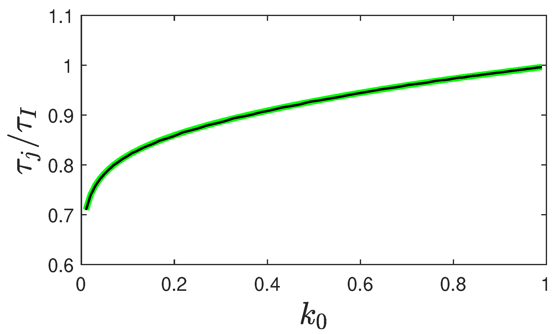
In Figure 7 the ratio τ j / τ I is displayed as a function of k 0 for η = 10 5 . The ratio always is smaller than unity demonstrating that the rate of new infections peaks before the fraction of infected persons in agreement also with the second and fourth columns in Figure 5.
Figure 7. Ratio of peak times. Numerical τ j / τ I = τ j / τ U (solid black) compared with this ratio using the analytical expression Equation (A15) with J 0 from Equation (A13) (thick green), which is well approximated by the simpler Equations (93) and (39) with Z s according to Equation (94). For this figure, η = 10 5 .
Preprints 138757 g007

5.2. Peak Time of Fraction of Infected Persons

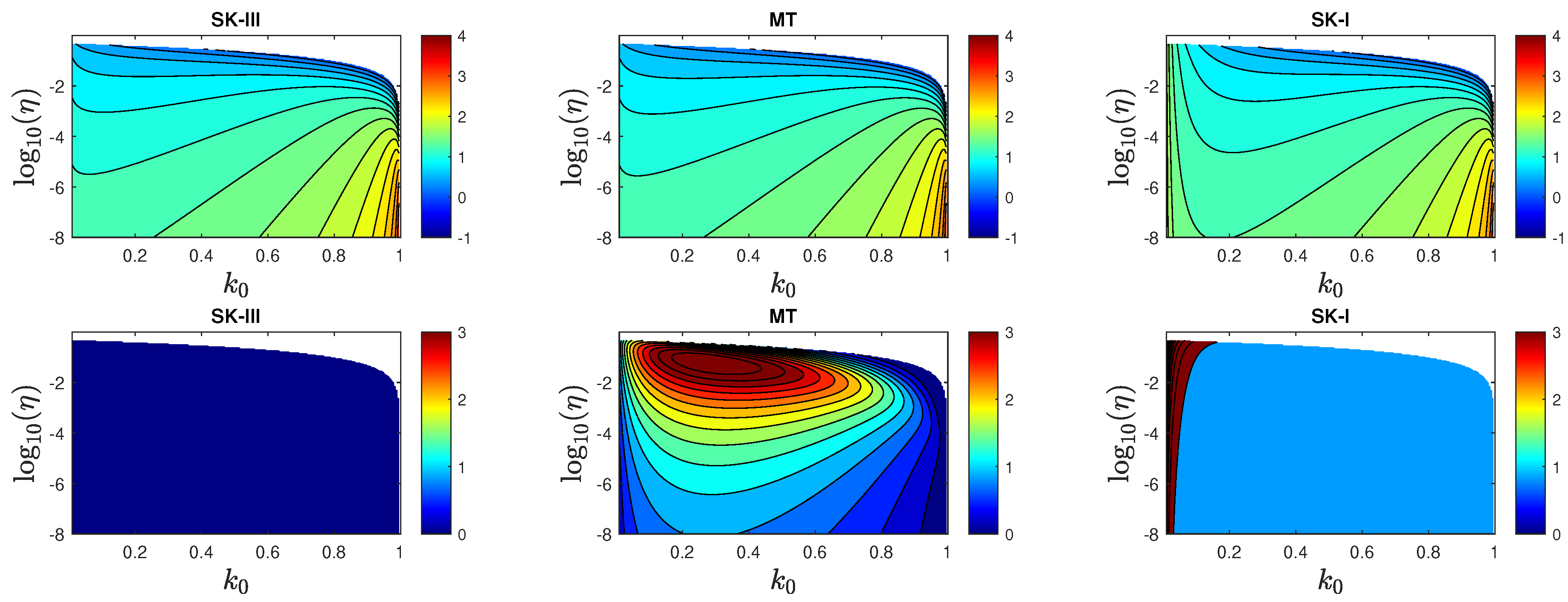
The peak time τ I of the fraction of infected persons is of particular interest [70,75,89,110,111,112,113,114,115,116,117,118,119,120]. According to Equation (50) this peak time τ I coincides with τ U given exactly by Equation (39). Consequently, we can compare this exact peak time with approximants derived before [103]. Figure 8 demonstrates in the first column that the analytical equation (38) coincides with the numerically calculated peak time τ I . While the earlier SK-I approximant (shown in the third column) provides acceptable agreement in a wide range of parameter values, the MT-approximant (shown in the second column) is less accurate.

6. Summary and Conclusions

We have derived a near-exact analytical solution of the statistical Susceptible-Infectious-Recovered (SIR) epidemics model for a constant ratio k 0 (referred to as KSSIR case) of infection ( a ( t ) ) to recovery ( μ ( t ) ) rates in the semi-time case which is particularly appropriate for modeling the temporal evolution of later (than the first) pandemic waves when a greater population fraction from the first wave has been infected. By introducing the dimensionless reduced time variable τ = t 0 t d ξ a ( ξ ) the derived solution holds for stationary rates as well as for the case of the same real time-dependency of the recovery and infection rates. The accuracy of the analytical solutions is confirmed by comparison with the exact numerical solutions of the SIR equations. Exact as well as accurately approximative solutions serve dual important purposes: first, they are suitable benchmarks for numerical codes, and secondly, they allow us to understand the fundamental behavior and functional patterns of epidemic outbursts as well as the decisive role of parameters.
The newly developed KSSIR-solution is not of inverse form as the known KSSIR solutions in the literature but rather directly expresses the three fractions S ( τ ) , I ( τ ) and R ( τ ) and thus the rate of new infections j ( τ ) = S ( τ ) I ( τ ) exactly in terms of the same function U ( τ ) = k 0 τ + 0 τ d x S ( x ) . With respect to the reduced time these fractions depend on two parameters: predominantly on the ratio k 0 and only weakly on the usually very small initial fraction η of infected persons. With respect to real time additionally the predescribed time dependent infection rate a ( t ) enters via the reduced time. These exact expressions involve the principal and non-principal branches of the Lambert functions, which routinely are available in mathematical software packages such as Python (scipy), Excel, Matlab and Mathematica, above and below the peak time of the function U ( τ ) which agrees with the peak time of the rate of infections I ( τ ) . The newly developed solution correctly reproduces all known exact expressions of the earlier KSSIR solution including the final values of S , I , and R . It also provides exact analytical formulas for the peak time τ I = τ U and the maximum fraction I max . These allow to check the accuracy of earlier derived approximants for τ I . In particular it is shown that the rate of new infections peaks before the fraction of infected persons.
The derived near-exact solution is not entirely exact because the reduced time dependence of U ( τ ) obeying a nonlinear integro-differential equation is only obtained approximately for small and large times with respect to τ U . At small reduced times where U ( τ ) 1 the approximation is based on the expansion of a double-exponential function to first-order, whereas at large reduced times an accurate simple approximation of the principal Lambert function W 0 ( Z ) is employed. The resulting rate of new infections correctly reproduces the known exact maximum rate of new infections.

Author Contributions

R.S.: conceptualization, methodology, formal analysis, writing-reviewing and editing; M.K.: methodology, formal analysis, software, writing-reviewing and editing, visualization. All authors have read and agreed to the published version of the manuscript.

Funding

This research received no external funding.

Informed Consent Statement

Not applicable.

Data Availability Statement

All data are enclosed with this publication.

Conflicts of Interest

The authors declare no conflict of interest

Appendix A. Inverse KSSIR-Solution of Earlier Work

For stationary ratios (18) Equation (7c) immediately integrates to
R ( τ ) = k 0 ln S ( τ ) 1 η = k 0 ln 1 J ( τ ) 1 η ,
where we used S ( τ ) = 1 J ( τ ) from Equation (10) so that also
I ( τ ) = d ln [ 1 J ( τ ) ] d τ
With these expressions the sum constraint (7c) then reads
J ( τ ) + d ln [ 1 J ( τ ) ] d τ + k 0 ln 1 J ( τ ) 1 η = 0 ,
implying
d J ( τ ) d τ = [ 1 J ( τ ) ] J ( τ ) + k 0 ln 1 J ( τ ) 1 η
With the initial condition J ( 0 ) = η Equation (A4) readily is solved in inverse form as
τ = η J d x ( 1 x ) [ x + k 0 ln 1 x 1 η ] .
This solution (A5) generalizes the known analytical solutions in the literature [1,2,121] as it holds for arbitrary time-dependence of the infection rate a ( t ) . The mentioned known solutions can be reproduced with Equation (A5) by setting τ = a 0 t on its left-hand side resulting from a constant injection rate a 0 .
Taking the derivative with respect to τ highlights the fact that the inverse integrand in (A5) is nothing but the differential rate of newly infected persons in terms of J ( τ ) , i.e.,
j ( τ ) = ( 1 J ( τ ) ) J ( τ ) + k 0 ln 1 J ( τ ) 1 η .
It has been noted before that important exact properties of the KSSIR-solution (A5) can be inferred without doing the inversion to J ( τ ) .

Appendix A.1. Final and Maximum Values

The solution (A5) indicates that the maximum value J = J ( τ = ) is attained when the denominator of the respective integrand vanishes, i.e.,
J + k 0 ln 1 J 1 η = 0 .
Consequently,
J = 1 + k 0 W 0 ( α ) ,
where W 0 is the principal solution of Lambert’s equation and
α = ( 1 η ) e 1 / k 0 k 0 .
The knowledge of J from Equation (A8) immediately yield
S = 1 J = k 0 W 0 ( α ) ,
R = k 0 ln 1 J 1 η = J ,
I = 1 S R = 0 , ,
j = j ( τ = ) = 0 .

Appendix A.2. Peak Differential Rate

Likewise, the maximum of the differential rate (A6) occurs when the derivative ( d j / d J ) J 0 = 0 vanishes. With Equation (A6) one finds
d j d J = 1 2 J k 0 [ 1 ln ( 1 η ) ] k 0 ln ( 1 J ) ,
yielding for J 0 the transcendental equation
2 J 0 = 1 k 0 + k 0 ln ( 1 η ) k 0 ln ( 1 J 0 ) ,
which is solved in terms of the non-principal Lambert function as
J 0 = 1 + k 0 2 W 1 ( α 0 ) , α 0 = 2 α e ,
with α from (A9). Inserting Equation (A13) in Equation (A6) and making use of Equation (A12) yields for the maximum value in reduced time
j max = j ( J 0 ) = ( 1 J 0 ) ( 1 J 0 k 0 ) = k 0 2 4 1 + W 1 ( α 0 ) 2 1
According to Equation (A5) the peak time of the differential rate (A6) is given by
τ j = η J 0 d x ( 1 x ) [ x + k 0 ln 1 x 1 η ] .
For a maximum to occur at finite positive times τ j > 0 , the derivative d j / d τ has to be positive at times 0 τ < τ j . With Equations (A11) - (A12) we readily find
d j d τ = d J d τ d j d J = j d j d J = j ( τ ) [ 1 2 J ( τ ) k 0 ( 1 ln ( 1 η ) ) k 0 ln ( 1 J ( τ ) ) ]   = j ( τ ) 2 ( J 0 J ( τ ) ) k 0 ln 1 J ( τ ) 1 J 0 .
Since the requirement of a maximum j max to exist at positive times is identical to the requirement of a positive d j / d τ at τ = 0 , we can insert J ( 0 ) = η into the last equality in the first line of Equation (A16) to find
d j d τ τ = 0 = η ( 1 η ) [ 1 2 η k 0 ] > 0
implying
k 0 < 1 2 η .
For inverse reproduction numbers k 0 greater than 1 2 η , the daily rate is monotonically decreasing at all times from its initial value j ( 0 ) = η ( 1 η ) (decay phase). Contrary, for k 0 < 1 2 η the daily rate of newly infected persons attains a maximum at a finite positive time (peak case). At k 0 = 1 2 η the daily rate starts in its maximum at τ = 0 , and then decreases, while S, R and J approach their final values below unity.

References

  1. Kermack, W.O.; McKendrick, A.G. A contribution to the mathematical theory of epidemics. Proc. Royal Soc. A 1927, 115, 700–721. [Google Scholar]
  2. Kendall, D.G. Deterministic and stochastic epidemics in closed populations. In Proc. Third Berkeley Symp. on Math. Statist. and Prob.; Univ. of Calif. Press, Berkeley, United States, 1956; Vol. 4, pp. 149–165.
  3. Babajanyan, S.G.; Cheong, K.H. Age-structured SIR model and resource growth dynamics: a Covid-19 study. Nonlinear Dynamics 2021, 104, 2853–2864. [Google Scholar] [CrossRef] [PubMed]
  4. Turkyilmazoglu, M. Explicit formulae for the peak time of an epidemic from the SIR model. Physica D-nonlinear Phenomena 2021, 422, 132902. [Google Scholar] [CrossRef] [PubMed]
  5. Telles, C.R.; Lopes, H.; Franco, D. SARS-COV-2: SIR Model Limitations and Predictive Constraints. Symmetry-basel 2021, 13, 676. [Google Scholar] [CrossRef]
  6. Carvalho, A.M.; Goncalves, S. An analytical solution for the Kermack-McKendrick model. Physica A 2021, 566, 125659. [Google Scholar] [CrossRef]
  7. Priesemann, V.; Brinkmann, M.M.; Ciesek, S.; Cuschieri, S.; Czypionka, T.; Giordano, G.; Gurdasani, D.; Hanson, C.; Hens, N.; Iftekhar, E.; Kelly-Irving, M.; Klimek, P.; Kretzschmar, M.; Peichl, A.; Perc, M.; Sannino, F.; Schernhammer, E.; Schmidt, A.; Staines, A.; Szczurek, E. Calling for pan-European commitment for rapid and sustained reduction in Sars-Cov-2 infections. Lancet 2021, 397, 92–93. [Google Scholar] [CrossRef]
  8. Mungkasi, S. Variational iteration and successive approximation methods for a SIR epidemic model with constant vaccination strategy. Applied Mathematical Modelling 2021, 90, 1–10. [Google Scholar] [CrossRef]
  9. dos Santos, I.F.F.; Almeida, G.M.A.; de Moura, F.A.B.F. Adaptive SIR model for propagation of Sars-Cov-2 in Brazil. Physica A 2021, 569, 125773. [Google Scholar] [CrossRef]
  10. Ghaffar, A.; Alanazi, S.; Alruwaili, M.; Sattar, M.U.; Ali, W.; Humayun, M.; Siddiqui, S.Y.; Ahmad, F.; Khan, M.A. Multi-Stage Intelligent Smart Lockdown using SIR Model to Control Covid 19. Intelligent Automation And Soft Computing 2021, 28, 429–445. [Google Scholar] [CrossRef]
  11. Law, K.B.; Peariasamy, K.M.; Gill, B.S.; Singh, S.; Sundram, B.M.; Rajendran, K.; Dass, S.C.; Lee, Y.L.; Goh, P.P.; Ibrahim, H.; Abdullah, N.H. Tracking the early depleting transmission dynamics of Covid-19 with a time-varying SIR model. Scientific Reports 2020, 10, 21721. [Google Scholar] [CrossRef]
  12. Brugnano, L.; Iavernaro, F.; Zanzottera, P. A multiregional extension of the SIR model, with application to the Covid-19 spread in Italy. Mathematical Methods In The Applied Sciences 2021, 44, 4414–4427. [Google Scholar] [CrossRef]
  13. Venkatasen, M.; Mathivanan, S.K.; Jayagopal, P.; Mani, P.; Rajendran, S.; Subramaniam, U.; Ramalingam, A.C.; Rajasekaran, V.A.; Indirajithu, A.; Sorakaya Somanathan, M. Forecasting of the Sars-Cov-2 epidemic in India using SIR model, flatten curve and herd immunity. Journal of Ambient Intelligence And Humanized Computing 2020. [Google Scholar] [CrossRef] [PubMed]
  14. Heng, K.; Althaus, C.L. The approximately universal shapes of epidemic curves in the Susceptible-Exposed-Infectious-Recovered (SEIR) model. Scientific Reports 2020, 10, 19365. [Google Scholar] [CrossRef] [PubMed]
  15. Chekroun, A.; Kuniya, T. Global threshold dynamics of aninfection age-structured SIR epidemic model with diffusion under the Dirichlet boundary condition. Journal of Differential Equations 2020, 269, 117–148. [Google Scholar] [CrossRef]
  16. Cadoni, M.; Gaeta, G. Size and timescale of epidemics in the SIR framework. Physica D-nonlinear Phenomena 2020, 411, 132626. [Google Scholar] [CrossRef]
  17. Chen, Y.C.; Lu, P.E.; Chang, C.S.; Liu, T.H. A Time-Dependent SIR Model for Covid-19 With Undetectable Infected Persons. Ieee Transactions On Network Science And Engineering 2020, 7, 3279–3294. [Google Scholar] [CrossRef]
  18. Cooper, I.; Mondal, A.; Antonopoulos, C.G. A SIR model assumption for the spread of Covid-19 in different communities. Chaos Solitons Fract. 2020, 139, 110057. [Google Scholar] [CrossRef]
  19. Karaji, P.T.; Nyamoradi, N. Analysis of a fractional SIR model with General incidence function. Appl. Math. Lett. 2020, 108, 106499. [Google Scholar] [CrossRef]
  20. McMahon, A.; Robb, N.C. Reinfection with Sars-Cov-2: Discrete SIR (Susceptible, Infected, Recovered) Modeling Using Empirical Infection Data. Jmir Public Health And Surveillance 2020, 6, 279–287. [Google Scholar] [CrossRef]
  21. Chen, X.; Li, J.; Xiao, C.; Yang, P. Numerical solution and parameter estimation for uncertain SIR model with application to Covid-19. Fuzzy Optimization And Decision Making 2021, 20, 189–208. [Google Scholar] [CrossRef]
  22. Ahmetolan, S.; Bilge, A.H.; Demirci, A.; Peker-Dobie, A.; Ergonul, O. What Can We Estimate From Fatality and Infectious Case Data Using the Susceptible-Infected-Removed (SIR) Model? A Case Study of Covid-19. Front. Med. 2020, 7, 556366. [Google Scholar] [CrossRef] [PubMed]
  23. Gopagoni, D.; Lakshmi, P., V. Susceptible, Infectious and Recovered (SIR Model) Predictive Model to Understand the Key Factors of Covid-19 Transmission. International Journal of Advanced Computer Science And Applications 2020, 11, 296–302. [Google Scholar] [CrossRef]
  24. Sene, N. SIR epidemic model with Mittag?Leffler fractional derivative. Chaos Solitons Fract. 2020, 137, 109833. [Google Scholar] [CrossRef]
  25. Mohamadou, Y.; Halidou, A.; Kapen, P.T. A review of mathematical modeling, artificial intelligence and datasets used in the study, prediction and management of Covid-19. Applied Intelligence 2020, 50, 3913–3925. [Google Scholar] [CrossRef]
  26. Barlow, N.S.; Weinstein, S.J. Accurate closed-form solution of the SIR epidemic model. Physica D-nonlinear Phenomena 2020, 408, 132540. [Google Scholar] [CrossRef]
  27. Simon, M. SIR epidemics with stochastic infectious periods. Stochastic Processes And Their Applications 2020, 130, 4252–4274. [Google Scholar] [CrossRef]
  28. Postnikov, E.B. Estimation of Covid-19 dynamics "on a back-of-envelope?: Does the simplest SIR model provide quantitative parameters and predictions? Chaos Solitons Fract. 2020, 135, 109841. [Google Scholar] [CrossRef]
  29. Shah, S.T.A.; Mansoor, M.; Mirza, A.F.; Dilshad, M.; Khan, M.I.; Farwa, R.; Khan, M.A.; Bilal, M.; Iqbal, H.M.N. Predicting Covid-19 Spread in Pakistan using the SIR Model. Journal of Pure And Applied Microbiology 2020, 14, 1423–1430. [Google Scholar] [CrossRef]
  30. Zhao, X.; He, X.; Feng, T.; Qiu, Z. A stochastic switched SIRS epidemic model with nonlinear incidence and vaccination: Stationary distribution and extinction. International Journal of Biomathematics 2020, 13, 2050020. [Google Scholar] [CrossRef]
  31. Richard, N.A.; Robert, D.; Valentin, D.; Emma, H.B.; Jan, A. Potential impact of seasonal forcing on a Sars-Cov-2 pandemic. Swiss Medical Weekly 2020, 150, w20224. [Google Scholar]
  32. Colombo, R.M.; Garavello, M. Optimizing vaccination strategies in an age structured SIR model. Mathematical Biosciences And Engineering 2020, 17, 1074–1089. [Google Scholar] [CrossRef] [PubMed]
  33. Samanta, S.; Sahoo, B.; Das, B. Dynamics of an epidemic system with prey herd behavior and alternative resource to predator. Journal of Physics A 2019, 52, 425601. [Google Scholar] [CrossRef]
  34. El Koufi, A.; Adnani, J.; Bennar, A.; Yousfi. Analysis of a Stochastic SIR Model with Vaccination and Nonlinear Incidence Rate. International Journal of Differential Equations 2019, 2019, 9275051. [Google Scholar] [CrossRef]
  35. Li, X.; Li, X.; Zhang, Q. Time to extinction and stationary distribution of a stochastic susceptible-infected-recovered-susceptible model with vaccination under. Mathematical Population Studies 2020, 27, 259–274. [Google Scholar] [CrossRef]
  36. Imron, C.; Hariyanto. ; Yunus, M.; Surjanto, S.D.; Dewi, N.A.C. Stability and persistence analysis on the epidemic model multi-region multi-patches. International Conference On Mathematics: Pure, Applied And Computation 2019, 1218, 012035. [Google Scholar]
  37. Britton, T.; Pardoux, E., Eds. Stochastic Epidemic Models with Inference; Vol. 2255, Springer, Berlin, 2019; pp. 1–472.
  38. Zhang, Y.; Li, Y.; Zhang, Q.; Li, A. Behavior of a stochastic SIR epidemic model with saturated incidence and vaccination rules. Physica A 2018, 501, 178–187. [Google Scholar] [CrossRef]
  39. Xu, C.; Li, X. The threshold of a stochastic delayed SIRS epidemic model with temporary immunity and vaccination. Chaos Solitons Fract. 2018, 111, 227–234. [Google Scholar] [CrossRef]
  40. Liu, Q.; Jiang, D.; Shi, N.; Hayat, T. Dynamics of a stochastic delayed SIR epidemic model with vaccination and double diseases driven by Levy jumps. Physica A 2018, 492, 2010–2018. [Google Scholar] [CrossRef]
  41. Witbooi, P.J. Stability of a Stochastic Model of an SIR Epidemic with Vaccination. Acta Biotheoretica 2017, 65, 151–165. [Google Scholar] [CrossRef]
  42. Miller, J.C. Mathematical models of SIR disease spread with combined non-sexual and sexual transmission routes. Infectious Disease Modelling 2017, 2, 35–55. [Google Scholar] [CrossRef]
  43. Jornet-Sanz, M.; Corberan-Vallet, A.; Santonja, F.J.; Villanueva, R.J. A Bayesian stochastic SIRS model with a vaccination strategy for the analysis of respiratory syncytial virus. Sort-statistics And Operations Research Transactions 2017, 41, 159–175. [Google Scholar]
  44. Estrada, E. Covid-19 and Sars-Cov-2, Modeling the present, looking at the future. Phys. Rep. 2020, 869, 1. [Google Scholar] [CrossRef] [PubMed]
  45. Schlickeiser, R.; Kröger, M. Determination of a key pandemic parameter of the SIR-epidemic model from past Covid-19 mutant waves and its variation for the validity of the Gaussian evolution. Physics 2023, 5, 205–214. [Google Scholar] [CrossRef]
  46. Schlickeiser, R.; Kröger, M. Analytical solution of the Susceptible-Infected-Recovered/Removed model for the not too late temporal evolution of epidemics for general time-dependent recovery and infection rates. Covid 2023, 3, 1781–1796. [Google Scholar] [CrossRef]
  47. Kröger, M.; Schlickeiser, R. Verification of the accuracy of the SIR model in forecasting based on the improved SIR model with a constant ratio of recovery to infection rate by comparing with monitored second wave data. R. Soc. Open Sci. 2021, 8, 211379. [Google Scholar] [CrossRef]
  48. Schlickeiser, R.; Kröger, M. Analytical solution of the SIR-model for the temporal evolution of epidemics. Part B. Semi-time case. J. Phys. A: Math. Theor. 2021, 54, 175601. [Google Scholar] [CrossRef]
  49. Guo, X.; Wang, J.L. A Unified Adsorption Kinetic Model Inspired by Epidemiological Model: Based on Adsorbates "Infect" Adsorbents. Langmuir 2024, 40, 15569–15579. [Google Scholar] [CrossRef]
  50. Guo, X.; Wang, J.L. A novel monolayer adsorption kinetic model based on adsorbates "infect" adsorbents inspired by epidemiological model. Water Research 2024, 253, 121313. [Google Scholar] [CrossRef]
  51. Cui, S.X.; Liu, F.Z.; Jardon-Kojakhmetov, H.; Cao, M. Discrete-time layered-network epidemics model with time-varying transition rates and multiple resources. Automatica 2024, 159, 111303. [Google Scholar] [CrossRef]
  52. Klemm, S.; Ravera, L. On SIR-type epidemiological models and population heterogeneity effects. Physica A 2023, 624, 128928. [Google Scholar] [CrossRef]
  53. Melikechi, O.; Young, A.L.; Tang, T.; Bowman, T.; Dunson, D.; Johndrow, J. Limits of epidemic prediction using SIR models. Journal of Mathematical Biology 2022, 85, 36. [Google Scholar] [CrossRef] [PubMed]
  54. Machado, G.; Baxter, G.J. Effect of initial infection size on a network susceptible-infected-recovered model. Physical Review E 2022, 106, 014307. [Google Scholar] [CrossRef] [PubMed]
  55. Yan, X.R. Research and Practice Analysis of Higher Vocational Colleges Facing the Experience and Dissemination of Regional Characteristic Tea Culture. Advances In Multimedia 2022, 2022, 2199788. [Google Scholar] [CrossRef]
  56. Jayatilaka, R.; Patel, R.; Brar, M.; Tang, Y.; Jisrawi, N.M.; Chishtie, F.; Drozd, J.; Valluri, S.R. A mathematical model of Covid-19 transmission. Materials Today-proceedings 2022, 54, 101–112. [Google Scholar] [CrossRef] [PubMed]
  57. Palomo-Briones, G.A.; Siller, M.; Grignard, A. An agent-based model of the dual causality between individual and collective behaviors in an epidemic. Computers In Biology And Medicine 2022, 141, 104995. [Google Scholar] [CrossRef]
  58. Roman, H.E.; Croccolo, F. Spreading of Infections on Network Models: Percolation Clusters and Random Trees. Mathematics 2021, 9, 3054. [Google Scholar] [CrossRef]
  59. Kavitha, C.; Gowrisankar, A.; Banerjee, S. The second and third waves in India: when will the pandemic be culminated? European Physical Journal Plus 2021, 136, 596. [Google Scholar] [CrossRef]
  60. Di Crescenzo, A.; Gomez-Corral, A.; Taipe, D. A computational approach to extreme values and related hitting probabilities in level-dependent quasi-birth-death processes. Mathematics And Computers In Simulation 2025, 228, 211–224. [Google Scholar] [CrossRef]
  61. Yu, C.; He, J.M.; Ma, Q.T.; Liu, X.Y. Dynamic Evolution Model of Internet Financial Public Opinion. Information 2024, 15, 433. [Google Scholar] [CrossRef]
  62. Athapaththu, D.V.; Ambagaspitiya, T.D.; Chamberlain, A.; Demase, D.; Harasin, E.; Hicks, R.; Mcintosh, D.; Minute, G.; Petzold, S.; Tefft, L.; Chen, J.X. Physical Chemistry Lab for Data Analysis of Covid-19 Spreading Kinetics in Different Countries. Journal of Chemical Education 2024, 101, 2892–2898. [Google Scholar] [CrossRef]
  63. Song, Z.L.; Zhang, Z.; Lyu, F.; Bishop, M.; Liu, J.K.; Chi, Z.H. From Individual Motivation to Geospatial Epidemiology: A Novel Approach Using Fuzzy Cognitive Maps and Agent-Based Modeling for Large-Scale. Sustainability 2024, 16, 5036. [Google Scholar] [CrossRef]
  64. Li, G.J.; Chang, B.F.; Zhao, J.; Wang, J.Y.; He, F.; Wang, Y.H.; Xu, T.; Zhou, Z.G. VIVIAN: virtual simulation and visual analysis of epidemic spread data. Journal of Visualization 2024, 27, 677–694. [Google Scholar] [CrossRef]
  65. Agosto, A.; Cerchiello, P. A data-driven test approach to identify Covid-19 surge phases: an alert-warning tool. Statistics 2024, 58, 422–436. [Google Scholar] [CrossRef]
  66. Yoon, I.; Ahn, C.; Ahn, S.; Lee, B.; Lee, J.; Park, M. Enhancing indoor building occupant safety in the built environment: Assessing the validity of social force modeling for simulating physical. Developments In The Built Environment 2024, 17, 100336. [Google Scholar] [CrossRef]
  67. Yadav, S.K.; Khan, S.A.; Tiwari, M.; Kumar, A.; Kumar, V.; Akhter, Y. Taking cues from machine learning, compartmental and time series models for Sars-Cov-2 omicron infection in Indian provinces. Spatial And Spatio-temporal Epidemiology 2024, 48, 100634. [Google Scholar] [CrossRef]
  68. Finney, L.; Amundsen, D.E. Asymptotic analysis of periodic solutions of the seasonal SIR model. Physica D-nonlinear Phenomena 2024, 458, 133996. [Google Scholar] [CrossRef]
  69. Rocha, J.L.; Carvalho, S.; Coimbra, B. Probabilistic Procedures for SIR and SIS Epidemic Dynamics on Erdös-Rényi Contact Networks. Appliedmath 2023, 3, 828–850. [Google Scholar] [CrossRef]
  70. Ilic, B.; Salom, I.; Djordjevic, M.; Djordjevic, M. An analytical framework for understanding infection progression under social mitigation measures. Nonlinear Dynamics 2023, 111, 22033–22053. [Google Scholar] [CrossRef]
  71. Atienza-Diez, I.; Seoane, L.F. Long- and short-term effects of cross-immunity in epidemic dynamics. Chaos Solitons Fract. 2023, 174, 113800. [Google Scholar] [CrossRef]
  72. Prodanov, D. Computational aspects of the approximate analytic solutions of the SIR model: applications to modelling of Covid-19 outbreaks. Nonlinear Dynamics 2023, 111, 15613–15631. [Google Scholar] [CrossRef]
  73. Darvishi, H.; Darvishi, M.T. An Analytical Study on Two High-Order Hybrid Methods to Solve Systems of Nonlinear Equations. Journal of Mathematics 2023, 2023, 9917774. [Google Scholar] [CrossRef]
  74. Karaji, P.T.; Nyamoradi, N.; Ahmad, B. Stability and bifurcations of an SIR model with a nonlinear incidence rate. Mathematical Methods In The Applied Sciences 2023, 46, 10850–10866. [Google Scholar] [CrossRef]
  75. Chakir, Y. Global approximate solution of SIR epidemic model with constant vaccination strategy. Chaos Solitons Fract. 2023, 169, 113323. [Google Scholar] [CrossRef]
  76. Salimipour, A.; Mehraban, T.; Ghafour, H.S.; Arshad, N.I.; Ebadi, M.J. SIR model for the spread of Covid-19: A case study. Operations Research Perspectives 2023, 10, 100265. [Google Scholar] [CrossRef]
  77. Luangwilai, T.; Thammawichai, M. Optimal river flow management to reduce flood risks: A case study in northeastern Thailand. River Research And Applications 2023, 39, 255–265. [Google Scholar] [CrossRef]
  78. Prodanov, D. Asymptotic analysis of the SIR model and the Gompertz distribution. Journal of Computational And Applied Mathematics 2023, 422, 114901. [Google Scholar] [CrossRef]
  79. Qin, Y.P.; Wang, Z.; Zou, L. Analytical properties and solutions of a modified Lindemann mechanism with three reaction rate constants. Journal of Mathematical Chemistry 2023, 61, 389–401. [Google Scholar] [CrossRef]
  80. Ishfaq, U.; Khan, H.U.; Iqbal, S. Identifying the influential nodes in complex social networks using centrality-based approach. Journal of King Saud University-computer And Information Sciences 2022, 34, 9376–9392. [Google Scholar] [CrossRef]
  81. Gairat, A.; Shcherbakov, V. Discrete SIR model on a homogeneous tree and its continuous limit. Journal of Physics A 2022, 55, 434004. [Google Scholar] [CrossRef]
  82. Al-Obaidi, R.H.; Darvishi, M.T. Constructing a Class of Frozen Jacobian Multi-Step Iterative Solvers for Systems of Nonlinear Equations. Mathematics 2022, 10, 2952. [Google Scholar] [CrossRef]
  83. Öz, Y. Analytical investigation of compartmental models and measure for reactions of governments. European Physical Journal E 2022, 45, 68. [Google Scholar] [CrossRef] [PubMed]
  84. de Souza, D.B.; Araújo, H.A.; Duarte, G.C.; Gaffney, E.A.; Santos, F.A.N.; Raposo, E.P. Fock-space approach to stochastic susceptible-infected-recovered models. Physical Review E 2022, 106, 014136. [Google Scholar] [CrossRef] [PubMed]
  85. Kozyreff, G. Asymptotic solutions of the SIR and SEIR models well above the epidemic threshold. Ima Journal of Applied Mathematics 2022, 87, 521–536. [Google Scholar] [CrossRef]
  86. Tchoumi, S.Y.; Rwezaura, H.; Tchuenche, J.M. Dynamic of a two-strain Covid-19 model with vaccination. Results In Physics 2022, 39, 105777. [Google Scholar] [CrossRef]
  87. Schwarzendahl, F.J.; Grauer, J.; Liebchen, B.; Löwen, H. Mutation induced infection waves in diseases like Covid-19. Scientific Reports 2022, 12, 9641. [Google Scholar] [CrossRef]
  88. Gulec, F.; Atakan, B.; Dressler, F. Mobile human ad hoc networks: A communication engineering viewpoint on interhuman airborne pathogen transmission. Nano Communication Networks 2022, 32-33, 100410. [Google Scholar] [CrossRef]
  89. Turkyilmazoglu, M. A restricted epidemic SIR model with elementary solutions. Physica A 2022, 600, 127570. [Google Scholar] [CrossRef]
  90. Turkyilmazoglu, M. An extended epidemic model with vaccination: Weak-immune SIRV I. Physica A 2022, 598, 127429. [Google Scholar] [CrossRef]
  91. d’Andrea, V.; Gallotti, R.; Castaldo, N.; De Domenico, M. Individual risk perception and empirical social structures shape the dynamics of infectious disease outbreaks. Plos Computational Biology 2022, 18, e1009760. [Google Scholar] [CrossRef]
  92. Jiang, J.Y.; Zhou, Y.C.; Chen, X.S.; Jhou, Y.R.; Zhao, L.Q.; Liu, S.; Yang, P.C.; Ahmar, J.; Wang, W. COVID-19 Surveiller: toward a robust and effective pandemic surveillance system basedon social media mining. Philosophical Transactions of The Royal Society A-mathematical Physical 2022, 380, 20210125. [Google Scholar] [CrossRef]
  93. Uçar, D.; Çelik, E. Analysis of Covid 19 disease with SIR model and Taylor matrix method. Aims Mathematics 2022, 7, 11188–11200. [Google Scholar] [CrossRef]
  94. Berenbrink, P.; Cooper, C.; Gava, C.; Marzagao, D.K.; Mallmann-Trenn, F.; Radzik, T. On Early Extinction and the Effect of Travelling in the SIR model. Uncertainty In Artificial Intelligence, Vol 180 2022, 180, 159–169. [Google Scholar]
  95. Hussain, S.; Madi, E.N.; Khan, H.; Etemad, S.; Rezapour, S.; Sitthiwirattham, T.; Patanarapeelert, N. Investigation of the Stochastic Modeling of Covid-19 with Environmental Noise from the Analytical and Numerical Point of View. Mathematics 2021, 9, 3122. [Google Scholar] [CrossRef]
  96. Rusu, A.C.; Emonet, R.; Farrahi, K. Modelling digital and manual contact tracing for Covid-19. Are low uptakes and missed contacts deal-breakers? Plos One 2021, 16, e0259969. [Google Scholar] [CrossRef]
  97. Lee, K.; Parish, E.J. Parameterized neural ordinary differential equations: applications to computational physics problems. Proceedings of The Royal Society A-mathematical Physical And Engineering 2021, 477, 20210162. [Google Scholar] [CrossRef]
  98. Bärwolff, G. A Local and Time Resolution of the Covid-19 Propagation-A Two-Dimensional Approach for Germany Including Diffusion Phenomena to. Physics 2021, 3, 536–548. [Google Scholar] [CrossRef]
  99. Kartono, A.; Karimah, S.V.; Wahyudi, S.T.; Setiawan, A.A.; Sofian, I. Forecasting the Long-Term Trends of Coronavirus Disease 2019 (COVID-19) Epidemic Using the Susceptible-Infectious-Recovered (SIR) Model. Infectious Disease Reports 2021, 13, 668–684. [Google Scholar] [CrossRef]
  100. Hynd, R.; Ikpe, D.; Pendleton, T. Two critical times for the SIR model. Journal of Mathematical Analysis And Applications 2022, 505, 125507. [Google Scholar] [CrossRef]
  101. Zhou, Y.C.; Jiang, J.Y.; Chen, X.S.; Wang, W. #StayHome or #Marathon? Social Media Enhanced Pandemic Surveillance on Spatial-temporal Dynamic Graphs. Proceedings of The 30th Acm International Conference On Information 2021, pp. 2738–2748.
  102. Schüttler, J.; Schlickeiser, R.; Schlickeiser, F.; Kröger, M. Covid-19 predictions using a Gauss model, based on data from April 2. Physics 2020, 2, 197–202. [Google Scholar] [CrossRef]
  103. Kröger, M.; Turkyilmazoglu, M.; Schlickeiser, R. Explicit formulae for the peak time of an epidemic from the SIR model. Which approximant to use? Physica D 2021, 425, 132981. [Google Scholar] [CrossRef]
  104. Lambert, J.H. Observations variae in Mathesin Puram, Acta Helvitica. Phys. Math. Anatom. Botan Med. 1758, 3, 128–168. [Google Scholar]
  105. Kröger, M.; Schlickeiser, R. Analytical solution of the SIR-model for the temporal evolution of epidemics. Part A: Time-independent reproduction factor. J. Phys. A: Math. Theor. 2020, 53, 505601. [Google Scholar] [CrossRef]
  106. Haas, F.; Kröger, M.; Schlickeiser, R. Multi-Hamiltonian structure of the epidemics model accounting for vaccinations and a suitable test for the accuracy of its numerical solvers. J. Phys. A 2022, 55, 225206. [Google Scholar] [CrossRef]
  107. Weisstein, E. The CRC Encyclopedia of Mathematics, Third Edition; Chapman and Hall/CRC Press, Boca Raton, Florida, United States, 2009.
  108. Beyer, W.H. CRC Standard Mathematical Tables, 28th ed.; CRC Press, Boca Raton, Florida, United States, 1987; p. 455.
  109. Shampine, L.F.; Reichelt, M.W. The MATLABODE suite. SIAM J. Sci. Comput. 1997, 18, 1–22. [Google Scholar] [CrossRef]
  110. Bender, C.; Ghosh, A.; Vakili, H.; Ghosh, P.; Ghosh, A.W. An effective drift-diffusion model for pandemic propagation and uncertainty prediction. Biophysical Reports 2024, 4, 100182. [Google Scholar] [CrossRef]
  111. Jang, G.H.; Kim, S.J.; Lee, M.J.; Son, S.W. Effectiveness of vaccination and quarantine policies to curb the spread of Covid-19. Physica A 2024, 637, 129580. [Google Scholar] [CrossRef]
  112. Gao, W.H.; Wang, Y.; Cao, J.D.; Liu, Y. Final epidemic size and critical times for susceptible-infectious-recovered models with a generalized contact rate. Chaos 2024, 34, 013152. [Google Scholar] [CrossRef]
  113. Dobie, A.P.; Bayrakal, A.; Or, M.E.; Bilge, A.H. Dynamics of Feline Coronavirus and FIP: A Compartmental Modeling Approach. Veterinary Medicine International 2023, 2023, 2721907. [Google Scholar] [CrossRef]
  114. Shirazian, M. A new acceleration of variational iteration method for initial value problems. Mathematics And Computers In Simulation 2023, 214, 246–259. [Google Scholar] [CrossRef]
  115. Turkyilmazoglu, M. A highly accurate peak time formula of epidemic outbreak from the SIR model. Chinese Journal of Physics 2023, 84, 39–50. [Google Scholar] [CrossRef]
  116. Alshammari, F.S. Analysis of SIRV I model with time dependent coefficients and the effect of vaccination on the transmission rate and Covid- 19 epidemic waves. Infectious Disease Modelling 2023, 8, 172–182. [Google Scholar] [CrossRef] [PubMed]
  117. Dimou, A.; Maragakis, M.; Argyrakis, P. A network SIRX model for the spreading of Covid-19. Physica A 2022, 590, 126746. [Google Scholar] [CrossRef] [PubMed]
  118. Wang, Q.B.; Wu, H. There exists the ’smartest’ movement rate to control the epidemic rather than ’city lockdown’? Applied Mathematical Modelling 2022, 106, 696–714. [Google Scholar] [CrossRef] [PubMed]
  119. Gölgeli, M. The contagion dynamics of vaccine skepticism. Hacettepe Journal of Mathematics And Statistics 2022, 51, 1697–1709. [Google Scholar] [CrossRef]
  120. Wang, S.F.; Ma, Z.H.; Li, X.H.; Qi, T. A generalized delay-induced SIRS epidemic model with relapse. Aims Mathematics 2022, 7, 6600–6618. [Google Scholar] [CrossRef]
  121. Harko, T.; Lobo, F.S.N.; Mak, M.K. Exact analytical solutions of the susceptible-infected-recovered (SIR) epidemic model and of the SIR model with equal death and birth rates. Appl. Math. Comput. 2014, 236, 184–194. [Google Scholar] [CrossRef]
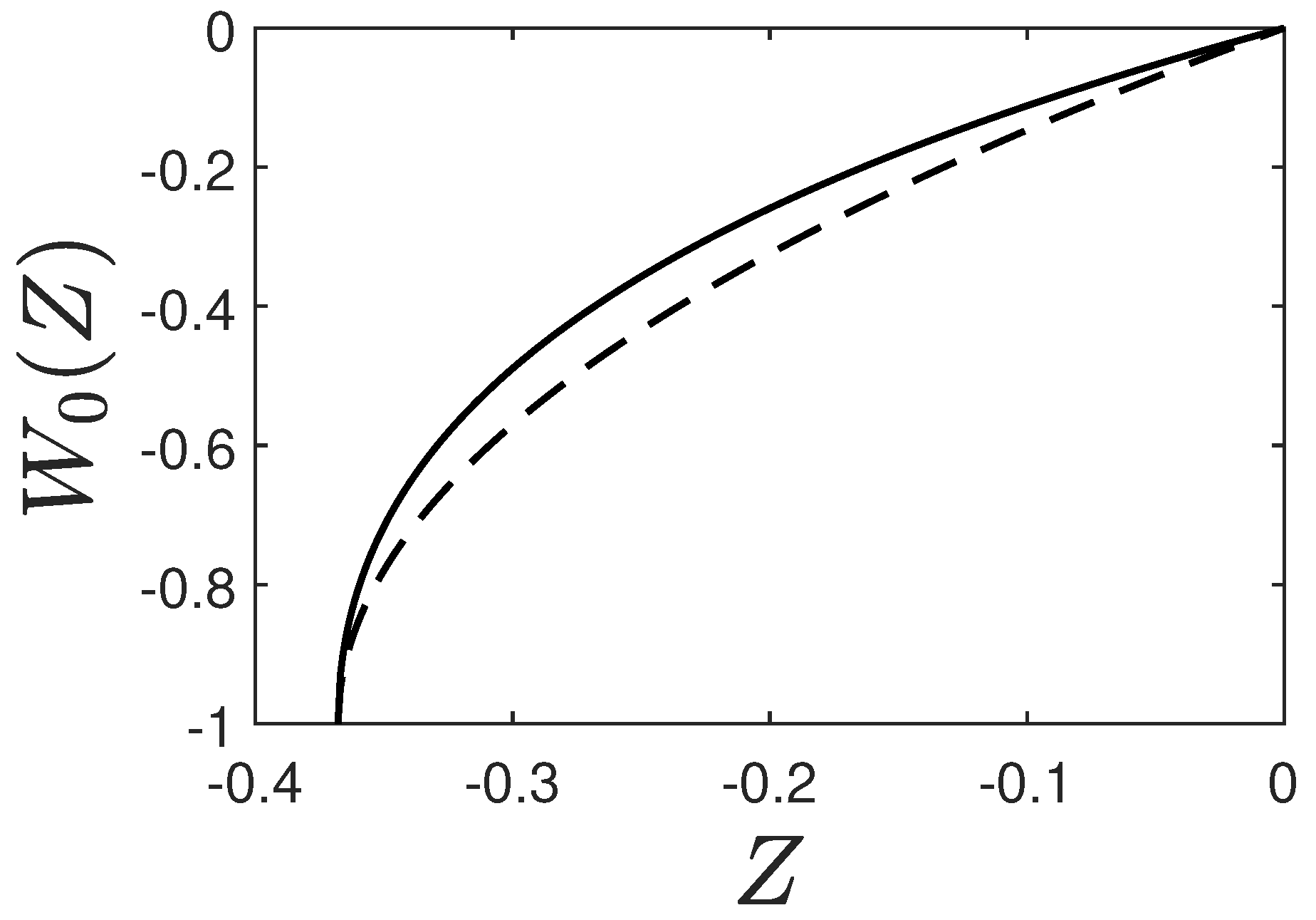
Figure 1. Principal branch of Lambert’s function. Approximation (57) (dashed) for W 0 ( Z ) (solid).
Preprints 138757 g001
Figure 2. Upper bound O ( k 0 ) = η e U max / k 0 versus k 0 for η = 10 5 . Shown is both the exact expression (black line) and the approximant (59) (green line). The dashed lines mark O ( k 0 ) = 1 . The curve is basically unaltered for smaller η .
Preprints 138757 g002
Figure 3. Limiting slope of U ( τ ) . Exact numerical result using Equation (43) and approximation (70). Following [106] the numerical solution of the GSL equations we obtained using the 10th order predictor–corrector Adams method [107,108]. Within 0.1% precision, a single-step solver based on a modified Rosenbrock formula of order 2, implemented by [109] as ode23s in MatlabTM yielded practically indistinguishable results.
Preprints 138757 g003
Figure 4. Limiting susceptible fraction. Exact (47) and approximate (72) analytic expressions for S . For this plot, η = 10 5 , but the situation is very comparable for any η 1 .
Preprints 138757 g004
Figure 8. Comparison of analytical approximants for τ I . The top row shows the decadic logarithm of τ I (colormap) versus k 0 and η for k 0 1 2 η , while the 2nd row shows the relative deviation (in %) between the exact τ I and the approximant. The first column displays the analytical τ I (39) (here denoted as SL-III), which coincides with the exact result, the second column the so-called MT-approximant proposed in Ref. [103], and the third column the SK-I-approximant [103].
Preprints 138757 g008
Disclaimer/Publisher’s Note: The statements, opinions and data contained in all publications are solely those of the individual author(s) and contributor(s) and not of MDPI and/or the editor(s). MDPI and/or the editor(s) disclaim responsibility for any injury to people or property resulting from any ideas, methods, instructions or products referred to in the content.
Copyright: This open access article is published under a Creative Commons CC BY 4.0 license, which permit the free download, distribution, and reuse, provided that the author and preprint are cited in any reuse.
Alerts
Prerpints.org logo

Preprints.org is a free preprint server supported by MDPI in Basel, Switzerland.

Subscribe

© 2025 MDPI (Basel, Switzerland) unless otherwise stated