
Submitted:
07 November 2024
Posted:
07 November 2024
You are already at the latest version
Abstract
The use of centrifugal pumps for water supply and distribution applications is evident in every industry as they efficiently transport fluid from a certain point. However, the sector faces severe concerns regarding its operating efficiency due to accumulated losses and sudden power consumption growth. Thus, it is crucial to find a remedy to mitigate these concerns and improve the performance of the centrifugal pump. This study aims to provide an improved design of centrifugal water pumps by analyzing the effects of changing its design parameters. Splitter blades, with a length of 80% of the main blade, will be included in the design. Using ANSYS software to generate a baseline design model, CFD analysis will be conducted. Then, an optimization study will be performed using the Response Surface Method (RSM) to formulate an optimized design. Results indicate that finding a perfect balance between the placement of the splitter blades, the design of the volute tongue clearance and thickness, and configuring the ellipse ratio of the splitter blades improves the pump's performance. The optimal design results in 27.35%, 15.70%, 28.18%, 16.67%, and 8.36% improvement in total efficiency, total head, static efficiency, static head, and power consumption, respectively.
Keywords:
centrifugal water pumps
; splitter blades
; CFD
; optimization
; RSM
1. Introduction
A centrifugal pump has proven itself to become an efficient piece of equipment often used in the everyday activities of an industry that involves the production of industrial goods and other necessities [1]. It is characterized by its simple design but provides high performance and pressure, which can be effectively used for the distribution and transportation of fluids. However, centrifugal pumps often consume vast amounts of energy in industrial applications to ensure the system operates smoothly [2]. This significantly affects global energy consumption; hence, many researchers have focused on providing solutions to improve pump efficiency to reduce energy consumption.
Given that the industry relies on using centrifugal pumps through various applications, the energy loss that comes with its actual production and operations is being ignored by people in the industry. Ignoring these details causes damage to the centrifugal pump but also causes severe concerns regarding its production capacity, leading to more serious economic problems. It is crucial to study the adjustment necessary to maintain the energy consumption of the centrifugal pump to a minimum [3]. In finding the best adjustment method, the areas of concern, such as unstable operation, lower operating efficiency, and energy waste, can fundamentally solve the massive problems of parametric losses of centrifugal pumps.
The trend for global energy consumption is expected to increase from 2016 to 2030 by 30%. The continuous increase in energy demand for industrial applications has been shown to contribute to the global energy consumption percentage increase. Based on the record, the pumps account for nearly 22% of the energy power supplied by electric motors in the world, whereas centrifugal pumps alone consume 16% of the total energy consumption for pumps, which is shown to be higher compared to other types of rotodynamic pumps [4]. Given this percentage of energy consumption of centrifugal pumps, the concern must be addressed to overcome the energy deficit and develop a feasible solution to identify energy-saving potential. It is known that centrifugal pumps consume excessive power due to accumulated losses that minimize the fluid flow and gradually affect the pump's performance. The cause of inefficiencies in the performance of the pump must be investigated to find optimal solutions, contributing to the development of a comprehensive design that will address the concern [5].
Existing research studies highlight the significance of modifying the impeller geometry to reduce the accumulated losses in the pump’s performance. Redesigning the impeller and changing the parameters of the blade profile improves the pump's hydraulic performance, leading to a more suitable design and adequate fluid flow. Simultaneously changing and altering the design of the impeller promotes a more uniform flow of fluid along the impeller passage [6,7]. Also, incorporating splitter blades in the design effectively improves the impeller outflow's stability and uniformity, reducing the inlet pressure pulsation. In general, splitter blades help decrease the clogging at the inlet of the impeller [8]. The result from a previous study concludes that an impeller with splitter blades improved the pump head by 8.2% while improving the overall efficiency by 3% [9]. This finding shows the relevance of considering the addition of splitter blades in the design of the impeller. However, blade regions, such as the trailing edge (TE) and leading edge (TE), should also be considered in the design as they affect the fluid flow within the pump. The TE profile of the blade is crucial for pressure pulsation, while the LE blade profile is vital for local flow separation and pressure distribution [10,11]. The impeller and the volute are the major components of a centrifugal pump. Hence, conducting a minor configuration on the volute should also be considered to have an efficient impeller-volute interaction, improving the hydraulic efficiency. A study observed that the spacing between the impeller outlet diameter and the location of the volute tongue causes a significant effect on the flow dynamics of the centrifugal pump [12]. Thus, minor changes in the volute tongue should also be investigated.
One of the best and most efficient ways of designing a centrifugal pump is using a computational fluid dynamics (CFD) approach. Present studies involving centrifugal pump design heavily rely upon the use of CFD for their respective design proposal as it is more efficient to use in a highly complex design having three-dimensional (3D) geometry models to use for simulating the behavioral flow and performance of the pump. Analyzing the flow of the centrifugal pump design is often a challenging task as it requires a critical understanding of a highly complex flow that is three-dimensional in nature [13]. Integrating CFD with the Response Surface Method (RSM) efficiently optimizes design. This approach is convenient for designing parameters with different variables to visualize the simulation trend in one diagram. Researchers have recently relied on using RSM, which has progressively been applied to find an optimized design for centrifugal pumps. The previous study employed RSM in their Pareto-based multi-objective optimization of centrifugal pump design to investigate the trend of the pump performance results of their research [14]. The RSM efficiently represented the system’s response as a function of one or more factors. The relationship of the parameters was displayed using RSM graphical techniques, allowing the researchers to identify the optimization area conveniently.
Achieving an optimal pump operation has been challenging in terms of minimizing energy costs and ensuring substantial head availability because the water supply and distribution system are heavy consumers of electrical energy [15]. Thus, the primary concern of this research study is to address the issues about the application of centrifugal pumps in water supply and distribution systems. In particular, this study aims to investigate the effects of modifying the impeller and the volute. Modifications in the impeller will incorporate splitter blades, varying their placement within the impeller and its TE and LE blade profiles, specifically at their corresponding ellipse ratios at the hub and shroud. On the other hand, minor modifications will be conducted in the volute, specifically the volute tongue thickness and clearance, to promote efficient impeller-volute interaction with the design. Since investigations from previous studies had consistently focused on redesigning the impeller and changing the number of blades, considering these additional factors offers a more thorough approach to developing an optimal centrifugal pump.
The centrifugal pump’s eminent suitability in the water supply and distribution industry accounts for an increase in excessive energy consumption. Thus, the significance of this study is to find a remedy for reducing the power consumption required to operate a centrifugal pump, especially in the continuous operation of the unit. In this way, people in the industry can save vast amounts of money on energy costs. The Response Surface Methodology will be utilized in the study to determine how the changes in input parameters affect the corresponding output results, which can be visualized in a 3D graph that can help interpret and understand the generated results of the study, leading to an optimized design. This also helps point out what design parameters must be considered or avoided to maintain the pump's performance at its best. Through this initiative, an optimized centrifugal pump design will also help decrease the power demand of the industrial sector that heavily relies on centrifugal pumps. This will also help address a small portion of the country's electricity crisis. Additionally, an optimized design of centrifugal pumps will lead to efficient equipment performance, reducing the cost of maintaining or changing the whole pump unit. Hence, the consumers and operators will be able to maximize the usable life of the pump and achieve desirable operational effectiveness.
The design configurations of this study highlight its use for water supply and distribution applications. The fluid nature considered in making the design was only intended for centrifugal pumps that carry water. With this, the proposed design may only be limited to centrifugal pumps for water supply and distribution applications and may not apply to other pump types and usage. The study's results will depend on the simulations made in computational fluid dynamics (CFD) software, which will focus on improving the flow of the fluid within the centrifugal pump by determining the pressure of the fluid within the pump and the pressure-induced in the meridional surface of the impeller blade along with the determination of the amount of turbulence present in the flow of the fluid. The CFD analysis that will be conducted will be limited to the normal condition of the water at one atmospheric pressure while neglecting the temperature changes in the water. Thus, the study will focus merely on the analysis of the flow of the fluid from the inlet to the outlet of the pump. Although the study intends to enhance the performance capabilities of centrifugal pumps, the findings of this research may still change if implemented and tested on an actual operation and scenarios. Hence, further validations are recommended for future research.
2. Methodology
The research methodology highlights two processes that will be conducted in the study. The initial process will be based on the implementation of computational fluid dynamics (CFD), followed by the optimization process of the design. These processes will allow us to examine the effect of varying parameters in a centrifugal pump and compare the results and performance of the baseline and optimized design models. Both the CFD and optimization processes will be conducted using ANSYS software. Figure 1 provides a summary of the whole research methodology.
2.1. CFD Simulation Process in Centrifugal Pump Design
This section will discuss the computational fluid dynamics (CFD) simulation process for designing a centrifugal pump. It will also give insight into how CFD was implemented in the design process, highlighting every step involved to have a complete overview of the procedures to be conducted in the study. The creation of geometry, which refers to creating three-dimensional (3D) models of the pump’s impeller and volute, will be the first to be discussed. This will be followed by parameterizing the pump components before proceeding with the geometry meshing. On the other hand, the pre-processing stage follows, which refers to finalizing the setup of the centrifugal pump before initializing the CFX-solver. Lastly, post-processing will also be presented to discuss the initial results of the baseline design of the centrifugal pump.
2.1.1. Geometric Modeling
The geometry of the pump’s impeller and volute can be generated by defining the parameters of the centrifugal pump through ANSYS Vista CPD. The selected reference for the design parameters was based on the study presented by Alawadhi et al. [16]. The input parameters will be utilized throughout the generation of the pump geometry up to the solver setup before the simulation. However, a few details will be changed for the selected reference, such as the number of vanes and impellers of the pump, as this study uses splitter blades for the design aspect. The chosen reference for the corresponding number of vanes was based on the study conducted by Gölcü et al. [17]. Though the first mentioned reference paper deals with a slurry classification of fluid, this study will dwell more on the effects of using these configurations in means of water as the selected type of fluid for the pump design. Moreover, the parameters used in this study are provided in Table 1:
After finalizing the parameters in Table 1, these data will be used in ANSYS Vista CPD to generate the design specifications of the corresponding impeller and volute, which will be used in creating the geometry profile of the two after the program has successfully computed and analyzed the given input. The impeller and volute specifications are based on the computational assessment of the program, which can be seen in Table 2 and Table 3. Also, the impeller export type setting was changed from isolated impeller to coupled to volute. This will ensure that the outlet radius of the impeller matches the inlet radius of the volute when exported from Vista CPD.
The geometry of the impeller can be extracted from ANSYS Vista CPD and transfer its data to BladeGen. The blade design extension of ANSYS BladeGen can be used to generate the three-dimensional (3D) model of the pump impeller. The splitter blades were also added to the impeller in this process, as shown in Figure 2 below:
The length of the splitter blades was reduced to 20% on the trailing edge (TE) side, as shown in the above figure. This is in line with the suggested design in the study conducted by Gölcü et al., where the length of the splitter blades at 80% of the length of the main blades shows a preferable result. Hence, the design suggestion was applied in this study. Additionally, the data from Vista CPD can be used to generate the geometry of the volute, which can be obtained through ANSYS DesignModeler. The generated geometry model of the volute is provided in Figure 3:
2.1.2. Parameterization
The TE and LE ellipse ratio at the hub and shroud, along with the splitter blade offset pitch fraction or the placement of the splitter blades between the two main blades, are the components to be parameterized for the pump impeller. On the other hand, the components to be parameterized in the volute are the cutwater or tongue thickness and clearance. The parameterization can be conducted through ANSYS DesignModeler, in which the software will define the selected components as the input parameters of the study. Figure 4 shows the location of the components to be parameterized in the design. In Figure 4a, the splitter offset pitch fraction refers to the placement of the splitter blades in the pump impeller. The initial value of the fraction was set to 0.5, which means the splitter blades are located between the main blades by default. A value less than 0.5 refers to the placement of the splitter blade close to the pressure side of the main blade, while a value greater than 0.5 refers to the splitter blade’s placement close to the main blade’s suction side. Figure 4b-c shows the TE and LE's ellipse ratio at the hub and shroud. These components will also be parameterized to determine their effect on the performance of the centrifugal pump, as an existing study shows that well-designed blade regions, such as an Ellipse on the Pressure Side (EPS) and Ellipse on Both Sides (EBS) profiles, contribute to improving the pump efficiency [18]. The modification of the EPS profile design was also observed to increase pump efficiency based on the study conducted by Zhang et al., which used an experimental approach with an impeller-volute combination [19]. Hence, configuring the ellipse ratio at the hub and shroud of TE and LE was also considered in this study. The volute tongue clearance and thickness were also parameterized in this study to improve the impeller-volute interaction further, leading to efficient hydraulic performance. This was based on Alemi et al.'s observation that the volute tongue significantly affects the absolute velocity in the impeller outflow [20]. Thus, redesigning the volute tongue was explicitly considered in the study of impeller-volute interaction. Figure 4d shows the location of the volute tongue parameters.
The initial values of the parameterized components for the impeller and volute were generated through the geometric modeling process. The corresponding initial values of the parameters are provided in Table 4.
2.1.3. Meshing
The impeller meshing process will be conducted through ANSYS CFX Fluid Flow and ANSYS Mechanical for the volute meshing. Both components share the same physics and solver preferences, CFD and CFX, respectively. Table 5 summarizes the mesh metrics for both the impeller and volute. The total nodes and elements generated based on the meshing processes of both components are provided in Table 6. Tu et al. highlight the importance of using an unstructured triangular mesh for further refinement in a complex geometry. Although structured mesh tends to generate highly skewed cells, this type of mesh generally leads to numerical unreliability that leads to the deterioration of computation results [21] (pp. 139-140). Hence, an unstructured (tetrahedral) type of mesh was used in the study. For best practice, a growth rate of 1.1-1.3 is typically used in centrifugal pump meshing. A value greater than 1.3 will give a coarse mesh, and a value lesser will provide a fine mesh.
The mesh metric in the previous table successfully meshed the pump impeller and volute. These parametric values must be defined to generate a mesh profile used in the CFX-pre setup. The meshed pump impeller and volute are shown in Figure 5.
2.1.4. Pre-Processing
The pre-processing stage of CFD simulation refers to combining the geometries of the pump impeller and volute. The mesh profiles of the two components will be imported to CFX Pre Setup to define the respective domains and their corresponding boundaries. The whole centrifugal pump setup was divided into two domains, namely S1 and R1. R1 refers to the rotating pump component, which generally contains boundaries such as the pump inlet, blade, hub, and shroud. The angular velocity was also defined in R1 at 1,600 RPM, the same speed used in Vista CPD. S1 refers to the stationary component of the pump, and this domain was used to define the pump volute. After determining the domain of the pump components, the interfaces were generated through Turbo Mode options. The turbo mode enables the system to completely define the connection of the two domains involved in the model. Also, Turbo Mode gives the option to choose the type of solver, kind of fluid, and flow rate. In this setup, the Shear-Stress Transport (SST) solver was used as default, water was selected as the fluid type, and the flow rate was 33.333 m3/s. The steady-state k–ω SST RANS model was selected throughout this study by default, as specified by the solver, as it gives highly accurate numerical predictions that determine the amount of flow separation under adverse pressure gradients. The k–ω SST turbulence model is an approach that combines both the strengths of the k–ω and k–ϵ models. Thus, an accurate prediction for flows and separations can be employed in complex structures [22]. The k–ω SST turbulence model was developed by Menter (1994), where it employs equations of the flow field such as the continuity and momentum equations [23]. The k–ω SST equation is defined through Equations (1-4):
Since the study will focus on the behavioral flow analysis of water within the pump, the material properties of water were set in its normal condition. Thus, physical changes such as the temperature and other properties of water within the pump will not be included. However, the pressure induced within the pump, the pressure distribution on its flow, and the amount of turbulence present in the fluid will be observed in the results of the CFD simulation. The material properties of water, as defined in the pre-processing setup, are listed in Table 7.
2.1.5. Post-Processing
The post-processing stage of CFD simulations refers to the results of the simulated baseline design model of the centrifugal pump through ANSYS CFX-Post. The pressure and velocity contour plot results can be acquired in post-processing. In this way, an initial evaluation of the simulated results can be conducted to understand the behavior and the performance of the centrifugal pump. The flow streamlines can also be accessed in the post-processing stage to evaluate the fluid flow pattern in the pump’s inlet and outlet. The pump and impeller report can also be generated, and the software will provide the corresponding data, such as the pump efficiencies, head, and power. These acquired data will be assigned as the output parameters in preparation for the optimization process. The results of the baseline design model of the centrifugal pump from the conducted CFD simulation are provided in Table 8.
2.2. Optimization Process in Centrifugal Pump Design
The defined input and output parameters from the conducted CFD simulation will be used to develop an optimized centrifugal pump design. The optimization process involves different procedures that will be followed according to the general workflow of the Response Surface Optimization (RSO) tool in ANSYS Workbench. Figure 6 provides a workflow summary of the optimization process using RSO.
2.2.1. Design of Experiments (DOE) Setup
The Design of Experiments (DOE) is the initial procedure for conducting an optimization process through ANSYS software. It is known to explore data through computational algorithms efficiently. In this process, design points are created based on the defined data parameters of the study. The DOE used was the ‘Custom + Sampling’ type. The central composite design (CCD) was initially considered for use in the study. However, this DOE type was found unsuitable for this study as it contains numerous parameters to be considered, resulting in a higher computational cost and much time to process the input and output parameters. This finding also aligned with the suggestion of a related study, where Custom + Sampling ensures much smoother data processing for the DOE matrix [24]. Since the Custom + Sampling method processed the complexity of the given parameters, this DOE type was used in the study. The total number of samples in this process was set to 15. With this, the DOE has generated 15 samples with different design parameters. The generated design points are provided in Table 9.
In Table 9, 15 design points are shown, and their corresponding system-generated input and output parameters are provided. The input and output data were identified through the following parameters name below:
-
Input Parameters:
- Spltr_OPF = Splitter offset pitch fraction
- LE_erh = Leading edge ellipse ratio at hub
- LE_ers = Leading edge ellipse ratio at shroud
- TE_erh = Trailing edge ellipse ratio at hub
- TE_ers = Trailing edge ellipse ratio at shroud
- clear = Volute tongue clearance
- thk = Volute tongue thickness
-
Output Parameters:
- = Total efficiency
- = Total head
- = Static efficiency
- = Static head
- = Shaft/Input Power
2.2.2. Response Surface Method
In this process, the software generates a surface by interpolating the design points created in the DOE process. The relationship between the input and output parameters of the created design points is statistically and numerically processed in RSM, and their response is shown through either a 2D, 2D slice, or 3D-graphical model. The type of response surface used in this study is the default response surface, ‘Genetic Aggregation.’ This type of response surface is ideal for optimization as it aims to find the suitable response level for each design point through an iterative genetic algorithm based on the preferred tolerance for the output parameters. The given tolerance for the response surface variables is provided in Table 10. It is essential to define the tolerance of the output parameters for the software to generate a reasonable response accurately. The tolerances were kept at a minimum value to retain the accuracy of finding a suitable response for the study.
2.2.3. Response Surface Method
The optimization process is the last procedure used in the study. It deals with further validating the response of each sample and producing 3 candidates with corresponding optimized design results. In this process, the objectives and constraints of the output parameters must be set to allow the software to perform an optimization study and find optimal design parameters for the centrifugal pump. The given objectives and constraints for the output parameters are provided in Table 11 below:
The data provided in the above table will then be processed by the optimization method known as The Multi-Objective Genetic Algorithm (MOGA), which is a variant of Non dominated Sorted Genetic Algorithm-II (NSGA-II), which aims to determine the optimum design based on the given objectives and constraints. The configuration initially generated 7,000 samples consisting of 1400 samples per iteration at a maximum of 20 iterations and 33,600 estimated evaluations. The optimization process configuration allows a maximum Pareto and stability percentages of 70% and 2%, respectively. The Pareto percentage measures the amount of change per iteration of the given objectives and constraints, while the stability percentage determines the stability of the convergent points. The process measured a Pareto percentage at 0.07% and a convergence stability of 1.62% with no reported failure per iteration. The solution of the defined objective and constraints converged after 13 iterations. The process was completed after 23,329 evaluations.
3. Results and Discussion
This section, which contains the pump data, such as the efficiencies, heads, and power, will discuss interpreting the study's results. Contour plots will also determine the pump's pressure and fluid flow behavior. The evaluation will begin with the results of the baseline or initial design of the centrifugal pump through CFD simulation and compare them to the findings gathered in the optimized design through RSM.
3.1. Baseline Design Results
The summary of the pump performance for the baseline design of the centrifugal pump was previously provided in Table 8. The generated total efficiency resulted in 58.458%, with a total head of 13.041. On the other hand, the static efficiency resulted in 40.592% with a static head of 11.621 m. The shaft power, or the pump’s input power, resulted in 16,246 watts. Here, the total efficiency includes the outlet velocity and the static pressure generated in the pump, while the static efficiency measures only the static pressure in the inlet and outlet of the pump, hence the difference in the results.
3.1.1. Results Validation
The acquired results were compared to the experimental results presented in the study by Gölcü et al. to validate the results of the baseline model obtained through CFD simulation. Both mentioned related study and CFD simulation used 5 main blades and 5 splitter blades in the design, with the length of the splitter blades making 80% of the length of the main blades. Both designs selected water as the fluid type. However, slight differences in the properties of water were observed. The reference study used a density of 998 kg/m3 at 20°C, while this study defined a density of 997 kg/m3 at 25°C. While these differences can be observed, it is expected that slight deviances can occur. The total efficiency of the CFD was compared to the data observed in the reference experimental study at 80% nondimensional splitter blade length, while the total head of the CFD was compared to the design parameter of the head as defined in the reference experimental study. As shown in Table 12, the results were validated with a percent difference of 0.97372% for the total efficiency and 0.31489% for the total head.
3.1.2. CFD Analysis of the Baseline Design Model
To understand what led to the simulated results of the baseline design model, a CFD analysis will be conducted to determine the fluid flow behavior within the pump. A series of contour plots and streamline diagrams will be provided in this section to provide an in-depth understanding of the root causes that affect the pump’s performance. This analysis is crucial in the design process of a centrifugal pump as it will determine not just the flow of the fluid but also the amount of turbulence and pressure present within the pump.
- Pressure contour plot
The pressure contour plot in Figure 7a shows the pressure contour plot of the baseline design model. The figure shows that the pressure distribution between the impeller and the volute is not uniform. The pressure contour in the volute is higher than the pressure obtained in the impeller. Additionally, a vast area in the impeller develops negative pressure. A sudden pressure drop may result in further damage to the blades. This unbalanced pressure distribution between the two components deteriorates the pump's performance. It risks obtaining several issues, such as an unstable flow due to pressure fluctuations, excessive stress on the components, and unstable pumping operation. When it comes to improving the design of a centrifugal pump, this specific issue should be addressed to improve the quality of the pump's performance. Thus, the optimization design process should achieve a uniform pressure distribution.
To understand the fluid’s interaction with the pressure side of the blade, the area averaged pressure contour plot on the meridional surface is provided in Figure 7b. Based on the figure, a negative pressure is evident in the middle section of the blade. This implies that the middle section of the blade is at risk of cavitation. Cavitation occurs when the local pressure drops below the fluid’s vapor pressure. In Newtonian fluids, such as water, cavitation can occur through small vapor-filled cavities or bubbles that form when the pressure suddenly drops to a negative value. Cavities in the impeller blade significantly affect the pump's performance and longevity. Thus, it is vital to address the issue of cavitation in impeller blades to maintain the efficiency and performance of the pump.
- 2.
- Volume rendering of the entire domain
The cloud contour plot of the entire domain can be accessed through volume rendering. The volume rendering helps visualize the three-dimensional (3D) representation of the internal structure within the whole domain of the simulated baseline centrifugal pump design. In Figure 8a, the accumulated pressure of the entire domain is not equally distributed. Imbalanced pressure distribution is evident between the pump impeller and the volute, judging by the color contour of the given domain. An equal pressure distribution is essential to maintaining the system's fluid pumping efficiency within its entire domain. In this case, pressure fluctuations will likely occur between the impeller and volute, affecting fluid flow within the pump. Additionally, the impeller-volute interaction gradually affects the pump performance. Hence, this uneven pressure distribution may lead to an inefficient pump performance. On the other hand, the eddy viscosity cloud contour in Figure 8b shows the number of eddies present in the entire system. Determination of the number of eddies in the system is essential as these accumulated eddies generate turbulence in the pump. Thus, many eddies result in higher turbulence in the system. Based on the given figure, spots of eddies can be seen within the pump impeller, containing a higher value of eddy viscosity compared to the other sections within the pump. It is also evident that the eddy viscosity gradient is unevenly distributed within the system. Given this situation, the fluid flows turbulently due to the number of eddies in the system. A higher amount of turbulence within the fluid flow may increase energy loss. This finding may also be the cause of the presence of cavitation in the impeller blade surface, as previously shown in Figure 7b. Additionally, the turbulence caused by the number of eddies disturbs the path of the fluid and causes a decrease in pressure. With this, the system will demand more pumping power to attain the desired flow performance. Thus, this will increase the input power delivered by the shaft.
- 3.
- Velocity streamline of the baseline design model
The velocity streamline diagram visualizes the flow path of the fluid. Figure 9 shows the pattern flow of the fluid from the inlet and the outlet of the impeller blades. It can be seen in the given figure that the flow of fluid deviates from the profile of the blade at some point. The flow of the fluid also forms an indefinite pattern, which depicts that the flow of the fluid in the impeller is inconsistent, and the velocity reduces due to the irregularity of the flow pattern of the fluid, which can also have a significant effect on the hydraulic efficiency and performance of the pump.
3.2. Optimization Result
The optimization result involves presenting the findings in the conducted optimization study through the response surface method (RSM). This will provide valuable insight into how the optimal design of the centrifugal pump was achieved by analyzing the effect of modifying the design, determining the response of varying the input parameters, and evaluating the improved design’s performance from the centrifugal pump’s baseline design model. With this, the study's objectives can be fulfilled, and an insightful conclusion and recommendation can be constructed.
3.2.1. Minimum and Maximum Generated Response
The minimum and maximum responses are generated through the response surface method (RSM) according to the given tolerances provided in Table 10. The response surface type Genetic Aggregation was used to create 90 refinement points having different input parameters with their corresponding output or response. The calculated minimum and maximum responses are shown in Table 13. The total efficiency gathered a minimum response of 53.527% and a maximum of 86.262%. The minimum response for the total head gathered a response of 6.9756 m and a maximum of 18.383 m. The calculated minimum and maximum response for the static efficiency are 33.893% and 58.479%, respectively. The static head obtained a minimum response of 4.9608 m and a maximum of 17.401 m. The shaft power obtained a minimum response of 4936.6 W and a maximum of 58.479 W. These generated responses are beneficial in the optimization study as they will help determine the effect of different variations of parameters. In this way, the objective of the study to develop an optimized centrifugal pump can be achieved.
3.2.2. Goodness of Fit (GOF) Chart
The Goodness of Fit (GOF) Chart in Figure 10 shows the relationship between the observed and the predicted values. This criterion measures the degree of proportionality of the two values and determines how close the two values are to each other. The horizontal axis represents the observed points from the design points generated in the DOE test environment, and the vertical represents the estimated or predicted points extracted from the RSM. A diagonal regression line assesses the relationship between the observed and the predicted points to determine whether the two indicate a strong fit. The observed and predicted values for the shaft power, total, and static efficiency are linear, as the scattered points of these parameters closely align with the diagonal regression line. This means that the two values obtained possess a strong similarity. However, both the total and static heads move slightly away from the regression line. This indicates that the relationship between the observed and predicted values for the total and static heads contains a small number of discrepancies. Nonetheless, the deviation between the observed and predicted values of the two heads is still tolerable as they converged within the regression line at some point in the GOF chart. With these findings, it can be verified that through the GOF chart, the observed and predicted values are adequate results.
3.2.3. Sensitivity Analysis
The sensitivity analysis can be formulated through the local sensitivity chart in RSM. The local sensitivity helps understand how sensitive an output response is to changes in specific input parameters, which is beneficial in optimizing an optimization process. This sensitivity analysis can be used to determine the impact of varying the input parameters on the output’s response. The chart typically shows a positive and a negative range. A positive value implies a positive relation between the input and output parameters, while a negative value suggests the opposite. This means that an increase in the input parameter reduces the output value. To further analyze the sensitivity of the parameters, the local sensitivity chart is provided in Figure 11, illustrating the sensitivity percentage between the input and output parameters. Based on the figure, increasing the splitter blade offset pitch fraction for total efficiency further decreases its output value. The same results can be seen for the total head, static efficiency, and static head. Increasing the ellipse ratio at the hub in the trailing edge increases the total efficiency. On the other hand, increasing the ellipse ratio at the hub in the leading edge is more suitable for increasing the total head, static efficiency, and static head. In terms of the volute tongue thickness and clearance, the same findings were extracted from the investigation of Morabito et al., where modifying the volute tongue affects the pump's performance. Thus making it the most crucial variable in the design modification of the volute [25]. In keeping the shaft power at a minimum level, increasing almost every input parameter will be beneficial since one of the study's objectives is to reduce the power consumption of the centrifugal pump.
3.2.4. Response Surface Charts
This section highlights the use of response surface charts to further understand how varying the input parameters affects the output parameters in a positive and negative way. The results provided by the response surface charts will be used to determine the appropriate design modifications that must be made to optimize and fully boost the performance of the centrifugal pump. Combining these positive modifications of the parameters will also help shed light on how the pump performance improved from its baseline design model.
- Splitter blade offset pitch fraction
Figure 12 provides the effect of varying the splitter blades' offset pitch fraction in different output parameters. Using these response charts, it will be easier to understand how the changes in the position of the splitter blades affect the pump's performance in terms of the power required to drive the shaft and the total static efficiency and head. When the value of the splitter blades' offset pitch fraction is greater than 0.5, the total efficiency, total head, static efficiency, and static head decrease. In contrast, these output values increase when the value of the splitter blade offset pitch fraction is lower than 0.5. Regarding the shaft power, the highest value was obtained when the pitch fraction was near 0.49 and gradually decreased as the pitch fraction decreased. The initial value of the pitch fraction was set at 0.5. This means that the location of the splitter blades lies between the pressure and the suction side of the main blade. A value less than 0.5 refers to the location of the splitter blade close to the pressure side of the main blade, while a value greater than 0.5 refers to the splitter blade’s location close to the main blade’s suction side. Based on the results, it is suggested that the position of the splitter blades should be maintained closer to the pressure side at a reasonable distance to maintain a high value of pump efficiency and head, which also leads to a decrease in the value required for the shaft power. This observation shared the same sentiment to the findings of Zakeralhoseini & Schiffmann [26].
- 2.
- Volute tongue thickness and clearance
The effect of modifying the volute tongue thickness and clearance was also observed in this section of the study. Figure 13 shows that the total efficiency, total head, static efficiency, and static head increase when the volute tongue thickness increases and the clearance is maintained to a minimum value, which, in this case, is at a value of 11.87 mm and is represented by a violet line in the response chart. On the other hand, the shaft power can be reduced when the tongue thickness is reduced with an increase in the tongue clearance. Based on the findings provided in the response charts, it is evident that a minor change in the volute tongue profile has a significant effect on the pump's performance. The result shows that the tongue thickness should increase while maintaining a lesser value for tongue clearance to attain a better pump performance. Thus, it is crucial to consider the perfect balance between the design of the volute tongue thickness and clearance to achieve high efficiency and head while maintaining a minimum amount of shaft power, as modifying these two parameters of the volute contributes to a better impeller-volute interaction that improves the volumetric efficiency of the pump. With this, friction losses and pressure fluctuations from fluid flow at the impeller and volute are reduced, leading to a desirable performance of the pump. This finding proves that instead of redesigning only the impeller blades, a minor volute modification should also be considered and not neglected when designing an efficient centrifugal pump.
- 3.
- Splitter blade’s LE and TE ellipse ratio
In this section, the effect of varying the splitter blade’s Leading edge (LE) and Trailing edge (TE) ellipse ratio at the hub and shroud on each output parameter will be determined. This will allow a suitable combination of LE and TE modification to be selected for the centrifugal pump's design optimization.
- Total Efficiency
Figure 14 shows the effect of varying the LE and TE ellipse ratio at the hub and shroud in the total efficiency. For the LE, the initial value of the ellipse ratio of the hub and shroud was set to 2 and 1 for the TE. Both response charts depict an increase in efficiency from their initial values when the ellipse ratio at the hub increases, and the ellipse ratio at the shroud decreases. However, a slight decrease in efficiency is evident in the TE response chart when the ellipse ratio at the hub decreases, and the ellipse ratio at the shroud maintains its initial value of 1. Additionally, minimum efficiencies are observed for the LE and TE response charts when the ellipse ratio at the hub and shroud are on their initial values.
- Total Head
The effect of configuring the splitter blades LE and TE to the total head of the pump can be observed by visualizing the response of the output parameters to the configured input parameters. Figure 15 shows the effect of varying the LE and TE ellipse ratio at the hub and shroud in the total head. The maximum head can be attained for both LE and TE if their corresponding ellipse ratio at the hub increases and the ratio at the shroud decreases. The results of the response charts for the total head are similar to the analysis mentioned in the total efficiency. However, in this case, the minimum head can be seen when the hub's LE ellipse ratio decreases and the shroud's ellipse ratio increases. Meanwhile, increasing the ellipse ratio at the hub and shroud minimizes the head in TE. In this analysis, it is evident that configuring the LE and TE of the splitter blades creates a significant impact on the total head of the pump. To attain a desirable total head of the pump, the results suggest that the LE and TE must be kept greater than the initial value of the ellipse ratio at the hub and less than the initial value of the ellipse ratio at the shroud.
- Static Efficiency
In Figure 16, the response surface charts show the response of the output parameter (static efficiency) to the changing input variables of LE and TE. The response of static efficiency is shown to be similar to the response of the total efficiency observed in the previous discussion. Based on the given response charts, the maximum static efficiency can be attained for both LE and TE when their corresponding ellipse ratio at the hub is greater than their initial value, and the ellipse ratio at the shroud should maintain a value lesser than their initial value. The minimum static efficiency can also be observed when the ellipse ratio at the hub and shroud for both LE and TE are at their respective initial values. Therefore, both the total and static efficiencies results suggest that the ellipse ratio at the hub and shroud for LE and TE should be drawn away from their respective initial values to ensure an increase in total and static efficiencies.
- Static Head
Figure 17 provides the LE and TE configuration response charts in line with the static head. Based on the response charts, the behavioral response of the static head shows to be similar to the response observed in the total head. The static head increases for both LE and TE when their respective ellipse ratio at the hub increases from their initial values. At the same time, the ellipse ratio at the shroud decreases from their initial values. However, it was also observed in the response chart of the TE that the static head can also increase if the ellipse ratio at the hub decreases from its initial value and the ellipse ratio at the shroud increases from its initial value. This new finding shows how sensitive the static head is to the configuration of the TE ellipse ratio. Hence, finding a suitable balance between the ellipse ratio of the splitter blade’s LE and TE is suggested when it comes to design modification to maintain a desirable value of static head.
- Shaft Power
One of the study’s objectives is to develop an optimized centrifugal pump design that will decrease the power consumption for the pump's operation. In Figure 18, the response chart of the LE shows that the shaft power can be reduced if the ellipse ratio at the hub and shroud both increase from their initial value of 2. In contrast, a value of 2.1 for the ellipse ratio at the hub and a decreasing value of the ellipse ratio at the shroud increase the shaft power. On the other hand, the TE response chart shows the shaft power reduction when the ellipse ratio at the hub was 1.06, and the ellipse ratio at the shroud was greater than its initial value of 1. Decreasing the ellipse ratio at the hub from its initial value while increasing the ellipse ratio at the shroud from its initial value will increase shaft power. Through these results, the limitations of the LE and TE modifications can be determined to develop a reduced power consumption for the pump. A suitable combination of LE and TE parameters should be carefully selected to attain the given objectives of the study.
3.2.5. Optimal Candidate Points
The optimization study generated three (3) candidate points with corresponding improvements for the centrifugal pump design. These candidate points could be determined through the defined objectives and constraints. The optimization process solution was able to run using the Multi-Objective Genetic Algorithm (MOGA) method, which aims to find optimal results out of all the generated design and response points from DOE and RSM, respectively. The optimization process ended with 23,239 evaluations at 13 iterations with no reported failures. Hence, the suggested candidate points are exemplary. The three candidate points with optimal input design parameters are provided in Table 14, while their corresponding output parameters are provided in Table 15. Based on the data, the first candidate point is the best option for this study as it contains the highest total and static efficiencies while having the lowest power consumption compared with the two other candidate points. However, candidate points 2 and 3 are also acceptable as these three points only possess a small number of discrepancies. Nonetheless, the parameters obtained in candidate point 1 will be used in this study.
3.3. Comparison of Results
In this section, the optimized design results will be compared to the baseline design model of the centrifugal pump. This will determine the improvement the optimized design achieved by comparing their performance and highlighting the crucial aspects in the acquired results. The comparison will include the analysis of pressure distribution, amount of turbulence, and streamline diagram of the two designs to highlight the improvement of the optimized design from the baseline design model.
Figure 19 shows the difference between the pressure contour of the baseline and the optimized design. An improved pressure distribution can be seen in the contour plot of the optimized design, where the amount of pressure in the impeller and the volute are closely similar compared to the pressure distribution of the baseline design. A uniform pressure distribution results in improved stability regarding the relative motion of the impeller and the volute. Hence, this results in further improvement of the pump's performance and the flow dynamics of the fluid within the pump.
In Figure 20, a sudden pressure drop can be seen in the meridional blade surface of the baseline design. A negative pressure can be seen at the middle section of the blade, which depicts a cavitation risk on the affected area. The optimized design improves based on its pressure contour, where negative pressure in the middle section is removed. This shows that a risk of cavitation is not likely to occur within the blades of the optimized design. When a pump operates without cavitation, it is expected to increase efficiency as the stress induced by the occurrence of cavitation is removed. The obtained improvement in efficiency translates to reduced energy consumption, which supports one of the study's objectives.
To visualize the amount of pressure inside the pump, the pressure cloud contour provides a clear representation of the pressure distribution for each pump component. Figure 21 shows the difference between the pressure distribution of the baseline design and the optimized design. A large gap of pressure between the impeller and the volute can be seen in the baseline design. This shows an imbalanced pressure distribution between the two main components of the pump. The imbalanced pressure attained in the baseline design contributes to the unsteady flow of the fluid due to an inconsistent transfer of energy. In the optimized design, the pressure distribution shows improvement as the impeller and the volute has a nearly similar amount of pressure attained, judging by the color contour of the optimized design. The impeller-volute interaction plays a crucial role in improving the pump's performance as it enhances the behavioral flow of the fluid. Therefore, a uniform pressure distribution between the volute and the impeller will reduce pressure fluctuation and increase the hydraulic efficiency of the pump.
The eddy viscosity contour plot of the baseline design and the optimized one is shown in Figure 22. The baseline design shows a higher eddy viscosity within its system. Green spots, which correspond to higher eddies, are present between the impeller blades of the pump. This means there is an excessive amount of turbulence in the impeller, which affects the flow of the fluid. In the optimized design, the number of eddies is reduced to a minimum level, which means that the turbulence affecting the fluid flow is reduced. The number of eddies is also well distributed compared to the baseline design. This corresponds to the amount of turbulence that results in an efficient change in pressure and velocity within the fluid, which leads to minimizing energy losses. Additionally, eliminating turbulence helps reduce the energy required to pump the fluid, reducing the work exerted by the system. Thus, more efficient power consumption can be achieved.
The difference in fluid flow between the baseline and the optimized design is shown in Figure 23. It is evident in the given figure that the flow of fluid was improved in the optimized design. The fluid flow in the baseline design forms an indefinite pattern, which depicts that the fluid flow in the impeller is inconsistent, and the velocity reduces due to the irregularity of the flow pattern of the fluid. This irregularity has a great effect on the pump, resulting in inefficient performance. In terms of the optimized design, the scattered flow pattern of the fluid is shown to be reduced, and the velocity of the affected flow path also improves, judging by the consistency of the flow from the tip of the impeller blades. Therefore, the optimized design promotes a better fluid flow pattern than the baseline design, as it depicts flow stability in the inlet and outlet of the impeller. This enhances the hydraulic efficiency of the pump as the optimized design contains a better flow path of the fluid.
To visualize the improvement of the flow behavior of the fluid, an overall view of the streamline is provided in Figure 24. The streamline diagram shows the fluid's behavior at the impeller and the pump's volute. In the baseline design model, huge gaps can be observed in the streamlines. Some areas are not entirely covered by these streamlines, which may result in a decrease in the velocity of the fluid. This finding may have caused the reduction of pressure distribution in the fluid flow, as observed in the previous results and discussions. On the other hand, the streamline diagram shown in the optimized design is highly compact compared to the streamline diagram of the baseline model. By looking closely at the difference between the two streamline diagrams, the fluid circulation is much more consistent on the optimized design compared to the fluid flow in the baseline design. The stableness of the flow in the optimized design results in an increase in the velocity of the fluid. This finding justifies how the pump's performance was improved judging by the behavior of the fluid within the pump.
To determine the percentage improvement of the optimized design from the baseline design, the comparison of results and their corresponding input parameters are listed in Table 16. The total efficiency obtained a 27.35% improvement with 15.70% on the total head. The static efficiency improved by 28.18%, with 16.67% on the static head. The optimized design achieved a reduced power consumption, with an 8.36% improvement.
4. Conclusions
After subsequent performance analysis and result observation between the baseline and optimized centrifugal pump design, an insightful conclusion can be formulated. The result established that the offset pitch fraction of the splitter blade should maintain a value of less than 0.5. This means that the placement of the splitter blade should be kept at a reasonable distance near the pressure side of the main blade. In doing so, an increase in the performance of the pump can be achieved. The impeller-volute interaction plays a crucial role in improving the performance of the pump. Thus, modifying the volute tongue and clearance will help achieve the study's objective. The performance of the pump can be improved when the volute tongue thickness increases while maintaining the tongue clearance at a minimum level. This improves the dynamics between the impeller and the volute, enhancing the pump's hydraulic efficiency. For the LE and TE ellipse ratio, improvement in the performance of the pump, such as the efficiency and head, was achieved when the ellipse ratio at the hub increased and the ellipse ratio at the shroud decreased from their initial values of 2 and 1 for LE and TE respectively. However, reducing the shaft power requires different LE and TE configurations. In LE, setting the ellipse ratio at the hub and shroud to a value greater than their initial value of 2 will help minimize the power required by the shaft. On the other hand, the TE ellipse ratio at the hub should maintain a value closer to 1.06, and an increasing value of the ellipse ratio at the shroud that is greater than 1 to minimize the shaft power. However, configuring the LE and TE of the splitter blades to reduce the shaft power to its full extent may compromise the efficiency and head due to the differences in their required configuration. Therefore, finding the perfect balance between these parameters is essential to achieve a desirable pump performance with conflicting parametric objectives and a single constraint. The optimal design of the study resulted in 27.35%, 15.70%, 28.18%, and 16.67% improvement in total efficiency, total head, static efficiency, and static head, respectively, while achieving an 8.36% decrease in power consumption.
5. Recommendation
The study employed numerical analysis to investigate the results and develop an optimal centrifugal pump design. With this, the acquired results of the study were solely based on numerical approximations. Thus, the outcome of implementing the study in a real-world situation may deviate from the findings gathered in this study. Future studies may incorporate other existing optimization techniques to determine which technique generates a solution relatively closer to the results when implemented in a real-world setup. It is also recommended that researchers consider the type of material to be used in the design of the pump’s impeller and volute in the scope of the study. In this way, the effects on the pump's performance can be observed when the stress induced in the material of the pump is reduced. Additionally, the study was performed under normal water conditions, and the change in temperature of the water was neglected. To conduct a complete evaluation of the behavior of the fluid within the pump, considering the changes in the properties of water, such as the temperature, should be included in the analysis. Moreover, future researchers may uncover other design alternatives that will reduce the computational time needed to generate the optimal solution for the study.
Author Contributions
Conceptualization, J.A.; methodology, J.A and J.H.; software, J.A.; investigation, J.A.; writing—original draft preparation, J.A.; writing—review and editing, J.H.; supervision, J.H.; project administration, J.H. All authors have read and agreed to the published version of the manuscript.
Funding
This research received no external funding.
Data Availability Statement
The raw data supporting the conclusions of this article will be made available by the authors on request.
Conflicts of Interest
The authors declare no conflicts of interest.
References
- Nguyen, V. T. T.; Vo, T. M. N. Centrifugal Pump Design: An Optimization. Eurasia Proceedings of Science, Technology, Engineering and Mathematics 2022, 17, 136–151. [Google Scholar] [CrossRef]
- Zhang, L.; Wang, X.; Wu, P.; Huang, B.; Wu, D. Optimization of a Centrifugal Pump to Improve Hydraulic Efficiency and Reduce Hydro-Induced Vibration. Energy 2023, 268, 126677. [Google Scholar] [CrossRef]
- Zhang, W.; An, L.; Li, X.; Chen, F.; Sun, L.; Wang, X.; Cai, J. Adjustment Method and Energy Consumption of Centrifugal Pump Based on Intelligent Optimization Algorithm. Energy Reports 2022, 8, 12272–12281. [Google Scholar] [CrossRef]
- Arun Shankar, V. K.; Umashankar, S.; Paramasivam, S.; Hanigovszki, N. A Comprehensive Review on Energy Efficiency Enhancement Initiatives in Centrifugal Pumping System. Appl Energy 2016, 181, 495–513. [Google Scholar] [CrossRef]
- Chen, W.; Li, Y.; Liu, Z.; Hong, Y. Understanding of Energy Conversion and Losses in a Centrifugal Pump Impeller. Energy 2023, 263. [Google Scholar] [CrossRef]
- Shojaeefard, M. H.; Saremian, S. Effects of Impeller Geometry Modification on Performance of Pump as Turbine in the Urban Water Distribution Network. Energy 2022, 255, 124550. [Google Scholar] [CrossRef]
- Shojaeefard, M. H.; Saremian, S. Analyzing the Impact of Blade Geometrical Parameters on Energy Recovery and Efficiency of Centrifugal Pump as Turbine Installed in the Pressure-Reducing Station. Energy 2024, 289, 130004. [Google Scholar] [CrossRef]
- Wu, C.; Pu, K.; Shi, P.; Wu, P.; Huang, B.; Wu, D. Blade Redesign Based on Secondary Flow Suppression to Improve the Dynamic Performance of a Centrifugal Pump. J Sound Vib 2023, 554, 117689. [Google Scholar] [CrossRef]
- Siddique, M. H.; Samad, A.; Hossain, S. Centrifugal Pump Performance Enhancement: Effect of Splitter Blade and Optimization. 2021, 236 (2), 391–402. [CrossRef]
- Gao, B.; Zhang, N.; Li, Z.; Ni, D.; Yang, M. G. Influence of the Blade Trailing Edge Profile on the Performance and Unsteady Pressure Pulsations in a Low Specific Speed Centrifugal Pump. Journal of Fluids Engineering, Transactions of the ASME 2016, 138 (5). [CrossRef]
- Tao, R.; Xiao, R.; Wang, Z. Influence of Blade Leading-Edge Shape on Cavitation in a Centrifugal Pump Impeller. Energies 2018, Vol. 11, Page 2588 2018, 11 (10), 2588. [CrossRef]
- Fernández Oro, J. M.; Barrio Perotti, R.; Galdo Vega, M.; González, J. Effect of the Radial Gap Size on the Deterministic Flow in a Centrifugal Pump Due to Impeller-Tongue Interactions. Energy 2023, 278, 127820. [Google Scholar] [CrossRef]
- Shah, S. R.; Jain, S. V.; Patel, R. N.; Lakhera, V. J. CFD for Centrifugal Pumps: A Review of the State-of-the-Art. Procedia Eng 2013, 51, 715–720. [Google Scholar] [CrossRef]
- Safikhani, H.; Khalkhali, A.; Farajpoor, M. Pareto Based Multi-Objective Optimization of Centrifugal Pumps Using CFD, Neural Networks and Genetic Algorithms. Engineering Applications of Computational Fluid Mechanics 2011, 5 (1), 37–48. [Google Scholar] [CrossRef]
- Brentan, B.; Mota, F.; Menapace, A.; Zanfei, A.; Meirelles, G. Optimizing Pump Operations in Water Distribution Networks: Balancing Energy Efficiency, Water Quality and Operational Constraints. Journal of Water Process Engineering 2024, 63, 105374. [Google Scholar] [CrossRef]
- Alawadhi, K.; Alzuwayer, B.; Mohammad, T. A.; Buhemdi, M. H. Design and Optimization of a Centrifugal Pump for Slurry Transport Using the Response Surface Method. Machines 2021, Vol. 9, Page 60 2021, 9, (3), 60. [Google Scholar] [CrossRef]
- Gölcü, M.; Usta, N.; Pancar, Y. Effects of Splitter Blades on Deep Well Pump Performance. J Energy Resour Technol 2007, 129 (3), 169–176. [Google Scholar] [CrossRef]
- Chen, B.; Qian, Y. Effects of Blade Suction Side Modification on Internal Flow Characteristics and Hydraulic Performance in a PIV Experimental Centrifugal Pump. Processes 2022, Vol. 10, Page 2479 2022, 10 (12), 2479. [Google Scholar] [CrossRef]
- Zhang, N.; Liu, X.; Gao, B.; Wang, X.; Xia, B. Effects of Modifying the Blade Trailing Edge Profile on Unsteady Pressure Pulsations and Flow Structures in a Centrifugal Pump. Int J Heat Fluid Flow 2019, 75, 227–238. [Google Scholar] [CrossRef]
- Alemi, H.; Nourbakhsh, S. A.; Raisee, M.; Najafi, A. F. Effect of the Volute Tongue Profile on the Performance of a Low Specific Speed Centrifugal Pump. Proceedings of the Institution of Mechanical Engineers, Part A: Journal of Power and Energy 2015, 229 (2), 210–220. [Google Scholar] [CrossRef]
- Tu, J.; Yeoh, G. H.; Liu, C.; Tao, Y. CFD Mesh Generation – A Practical Guideline. In Computational Fluid Dynamics; Butterworth-Heinemann, 2024; pp 123–151. [CrossRef]
- Hu, P.; Li, Y.; Cai, C. S.; Liao, H.; Xu, G. J. Numerical Simulation of the Neutral Equilibrium Atmospheric Boundary Layer Using the SST K-ω Turbulence Model. Wind and Structures, An International Journal 2013, 17 (1), 87–105. [Google Scholar] [CrossRef]
- Menter, F. R. Two-Equation Eddy-Viscosity Turbulence Models for Engineering Applications. AIAA Journal 1994, 32 (8), 1598–1605. [Google Scholar] [CrossRef]
- Pagayona, E.; Honra, J. Multi-Criteria Response Surface Optimization of Centrifugal Pump Performance Using CFD for Wastewater Application. Modelling 2024, Vol. 5, Pages 673-693 2024, 5 (3), 673–693. [Google Scholar] [CrossRef]
- Morabito, A.; Vagnoni, E.; Di Matteo, M.; Hendrick, P. Numerical Investigation on the Volute Cutwater for Pumps Running in Turbine Mode. Renew Energy 2021, 175, 807–824. [Google Scholar] [CrossRef]
- Zakeralhoseini, S.; Schiffmann, J. The Influence of Splitter Blades and Meridional Profiles on the Performance of Small-Scale Turbopumps for ORC Applications; Analysis, Neural Network Modeling and Optimization. Thermal Science and Engineering Progress 2023, 39, 101734. [Google Scholar] [CrossRef]
Figure 1.
The methodological framework of the study.
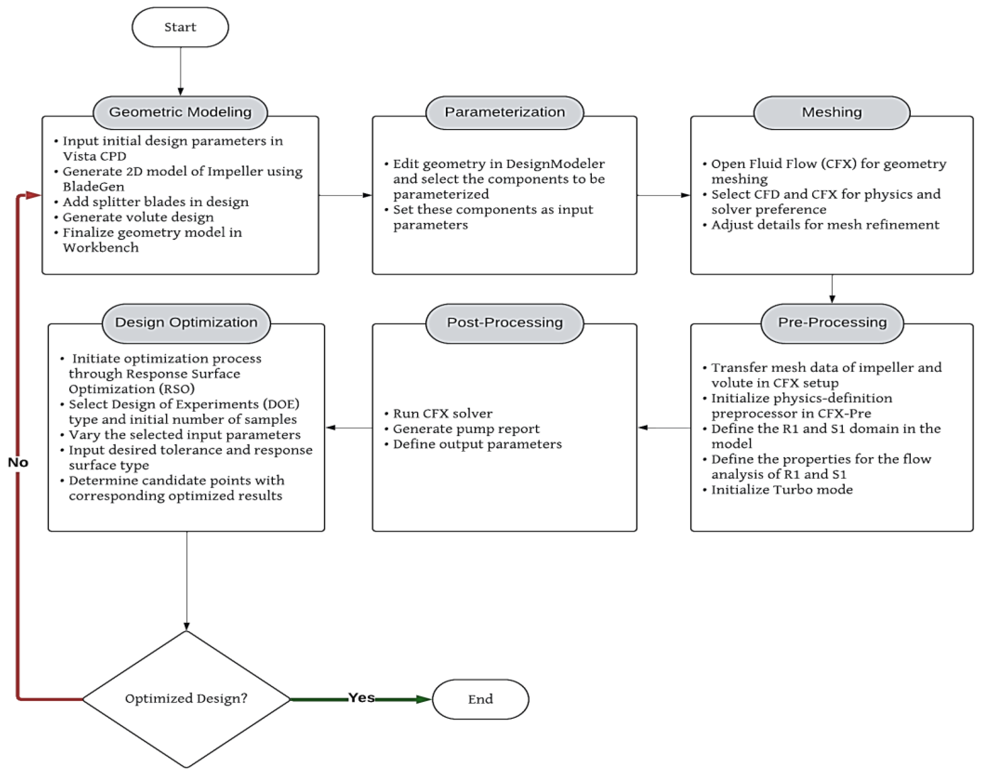
Figure 2.
Blade profile and 3D model of the pump impeller.
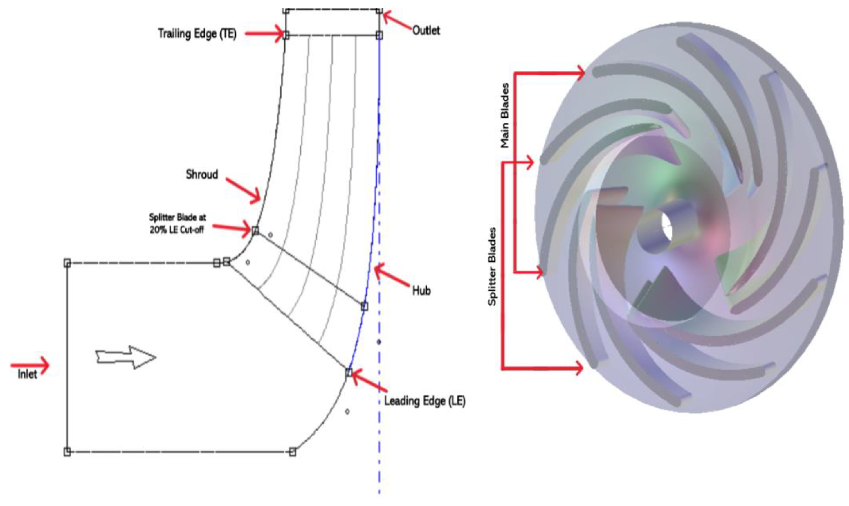
Figure 3.
3D model of the pump volute.
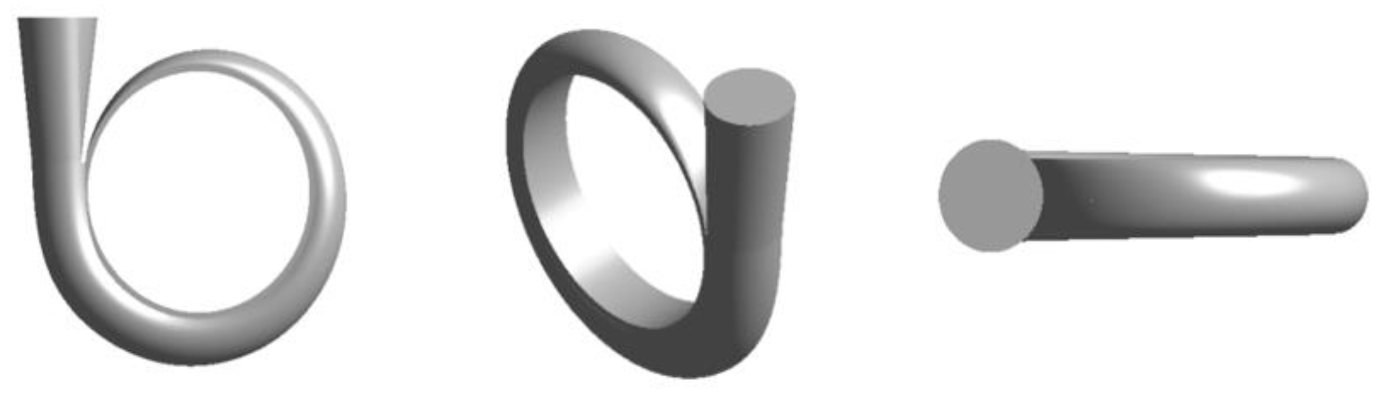
Figure 4.
Components to be parameterized: (a) splitter offset pitch fraction; (b) TE ellipse ratio at hub and shroud; (c) LE ellipse ratio at hub and shroud; (d) Volute tongue clearance and thickness.
Figure 4.
Components to be parameterized: (a) splitter offset pitch fraction; (b) TE ellipse ratio at hub and shroud; (c) LE ellipse ratio at hub and shroud; (d) Volute tongue clearance and thickness.
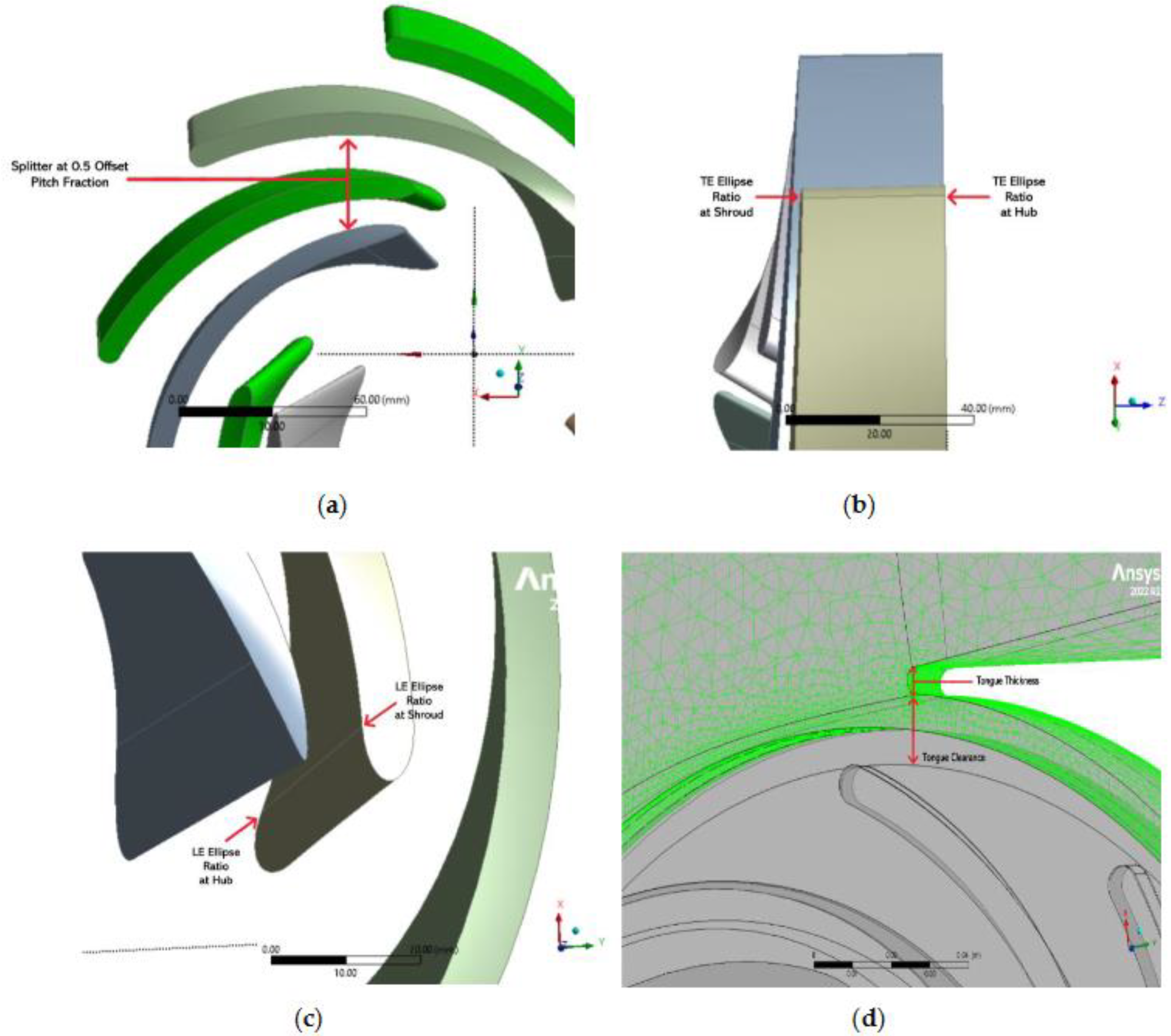
Figure 5.
Meshed model of the pump impeller and volute.
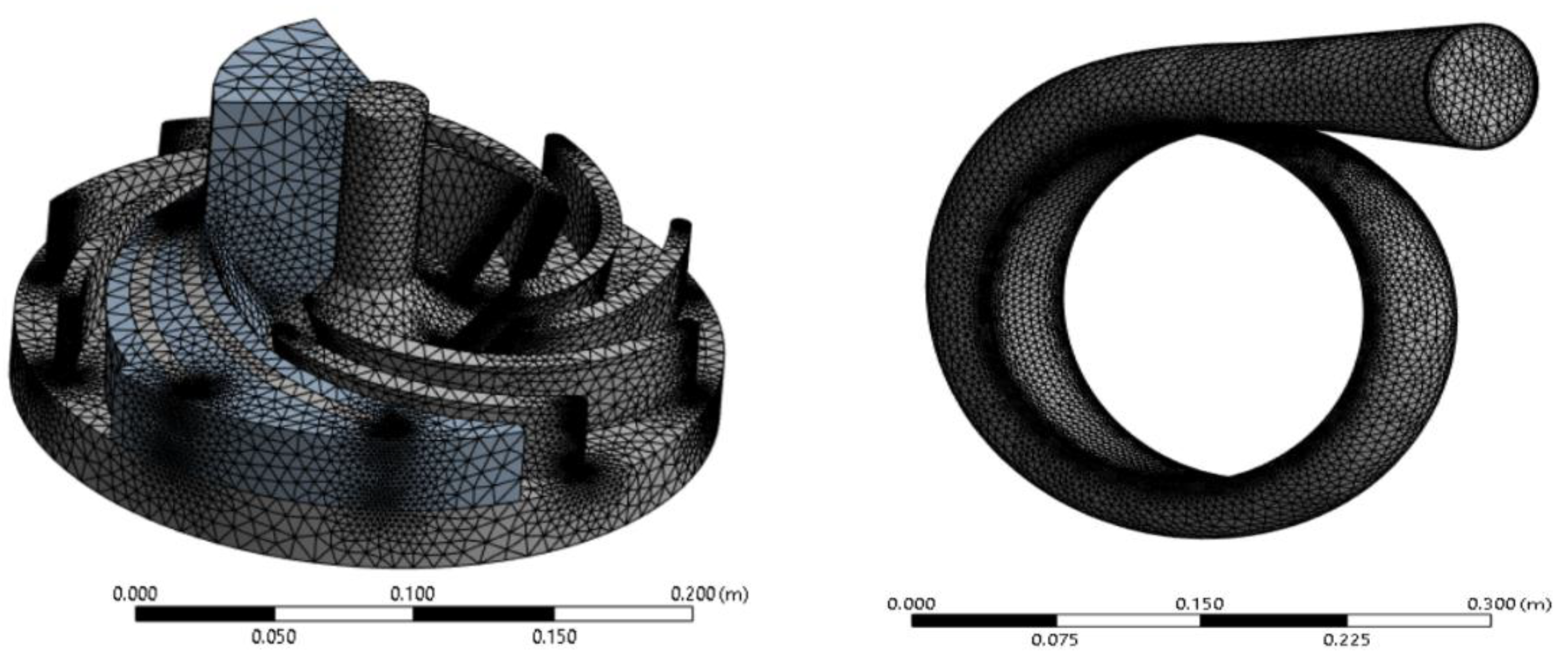
Figure 6.
Workflow summary of the optimization process.
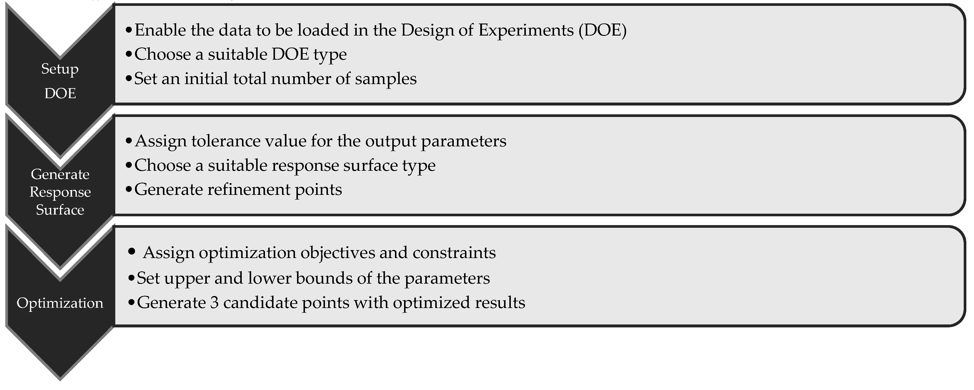
Figure 7.
The (a) pressure contour plot of the baseline design model and the (b) area-averaged pressure contour on the meridional surface of the blade.
Figure 7.
The (a) pressure contour plot of the baseline design model and the (b) area-averaged pressure contour on the meridional surface of the blade.

Figure 8.
The (a) pressure and (b) eddy viscosity cloud contour of the entire domain.
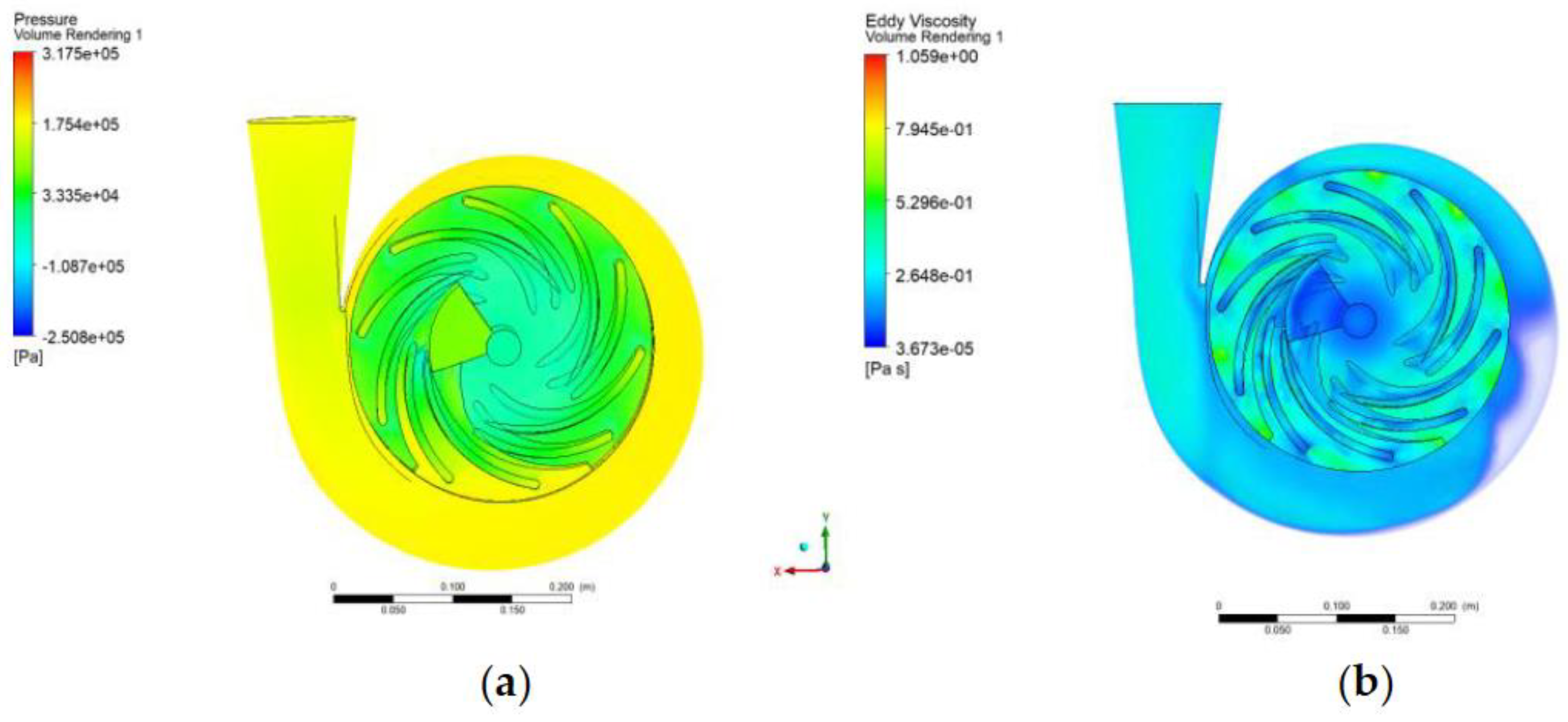
Figure 9.
The velocity streamline diagram of the baseline design model.
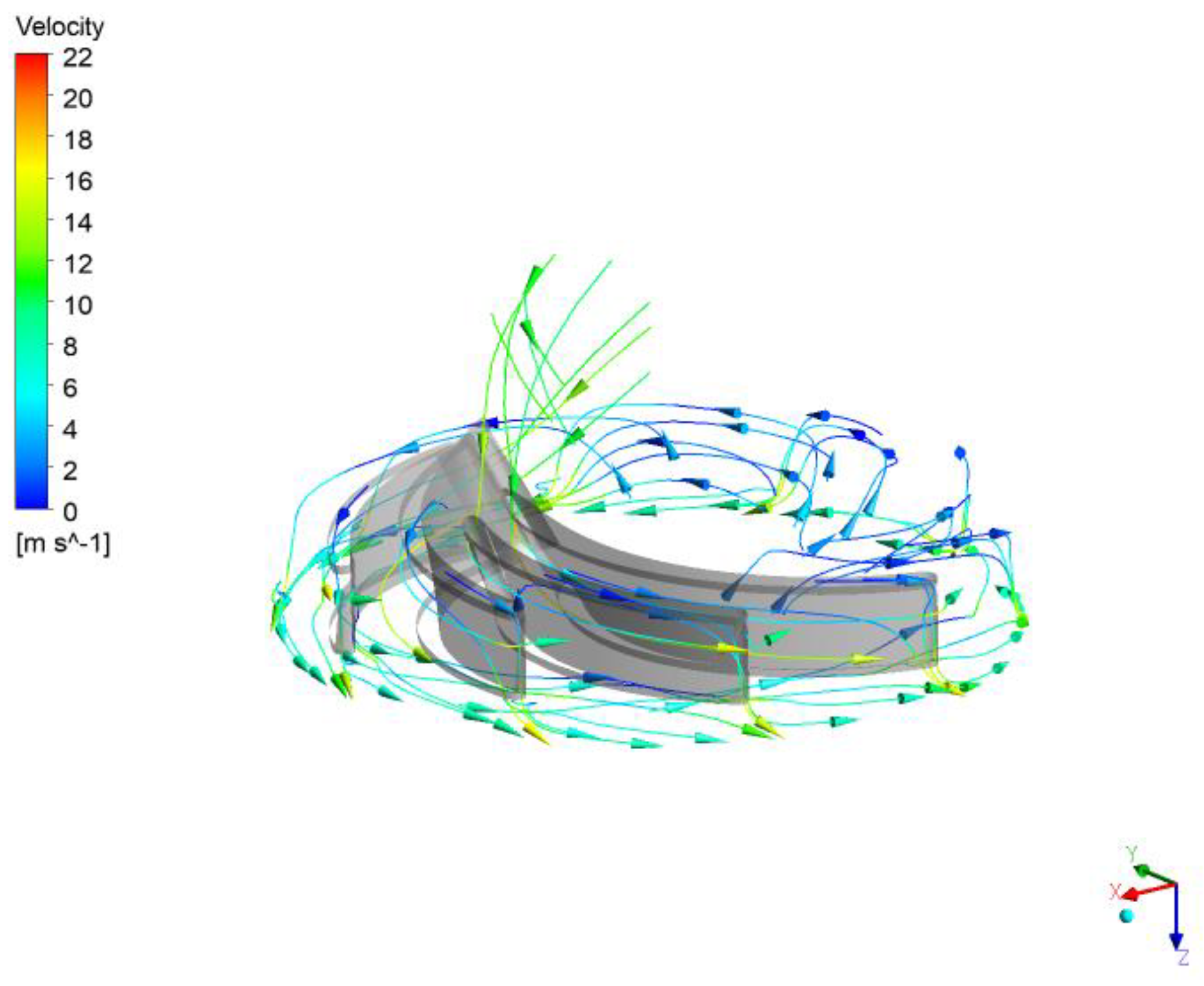
Figure 10.
Normalized value chat of the predicted vs. observed values of the study.
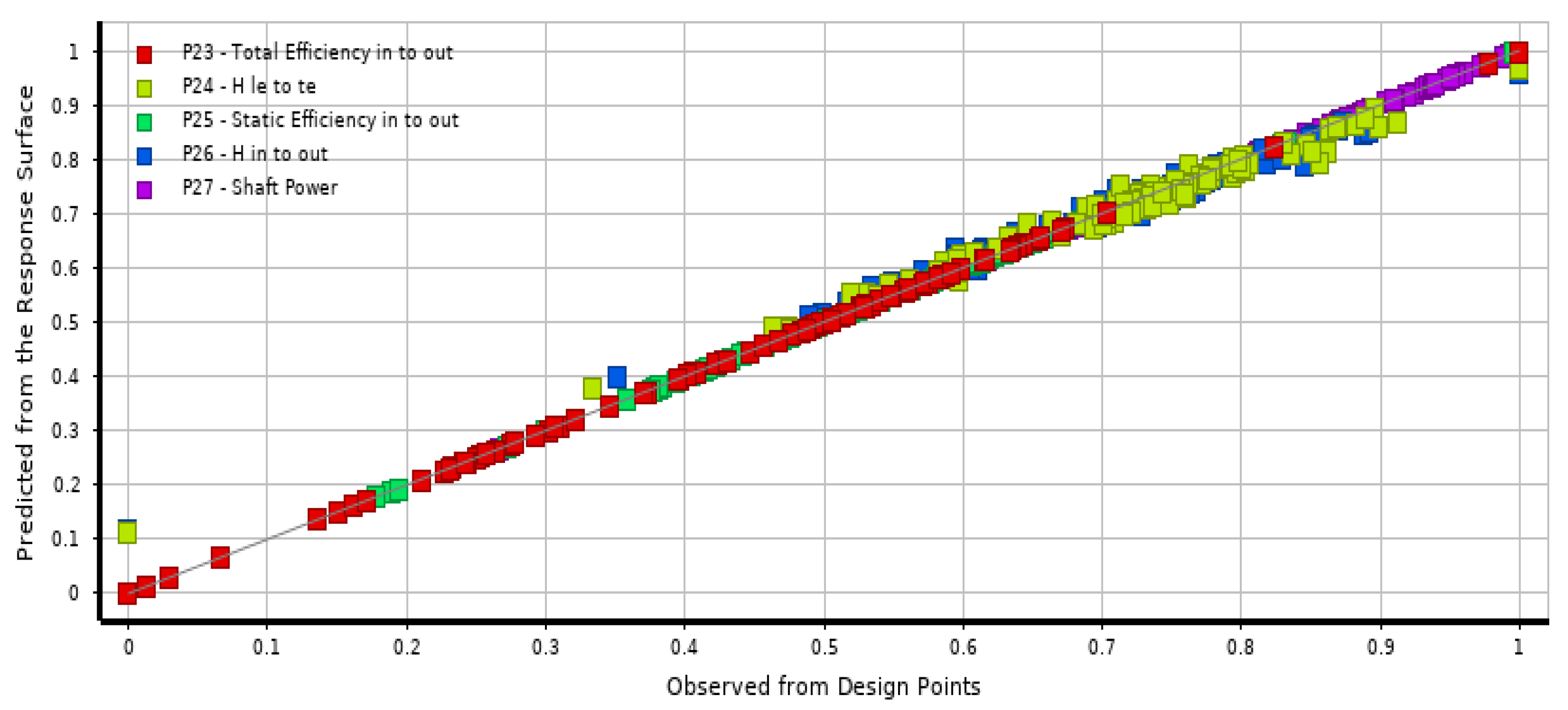
Figure 11.
Local sensitivity chart of the input and output parameters.
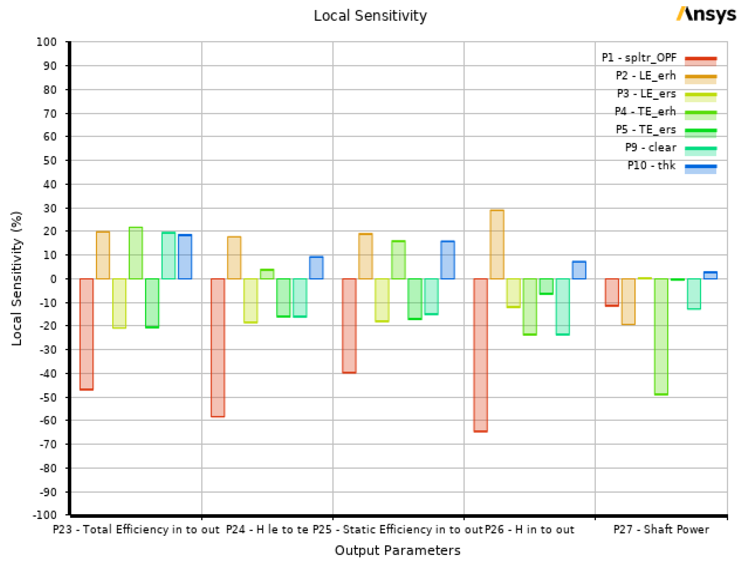
Figure 12.
The effect of varying splitter blades offset pitch fraction in (a) total efficiency; (b) total head; (c) static efficiency; (d) static head; (e) shaft power.
Figure 12.
The effect of varying splitter blades offset pitch fraction in (a) total efficiency; (b) total head; (c) static efficiency; (d) static head; (e) shaft power.
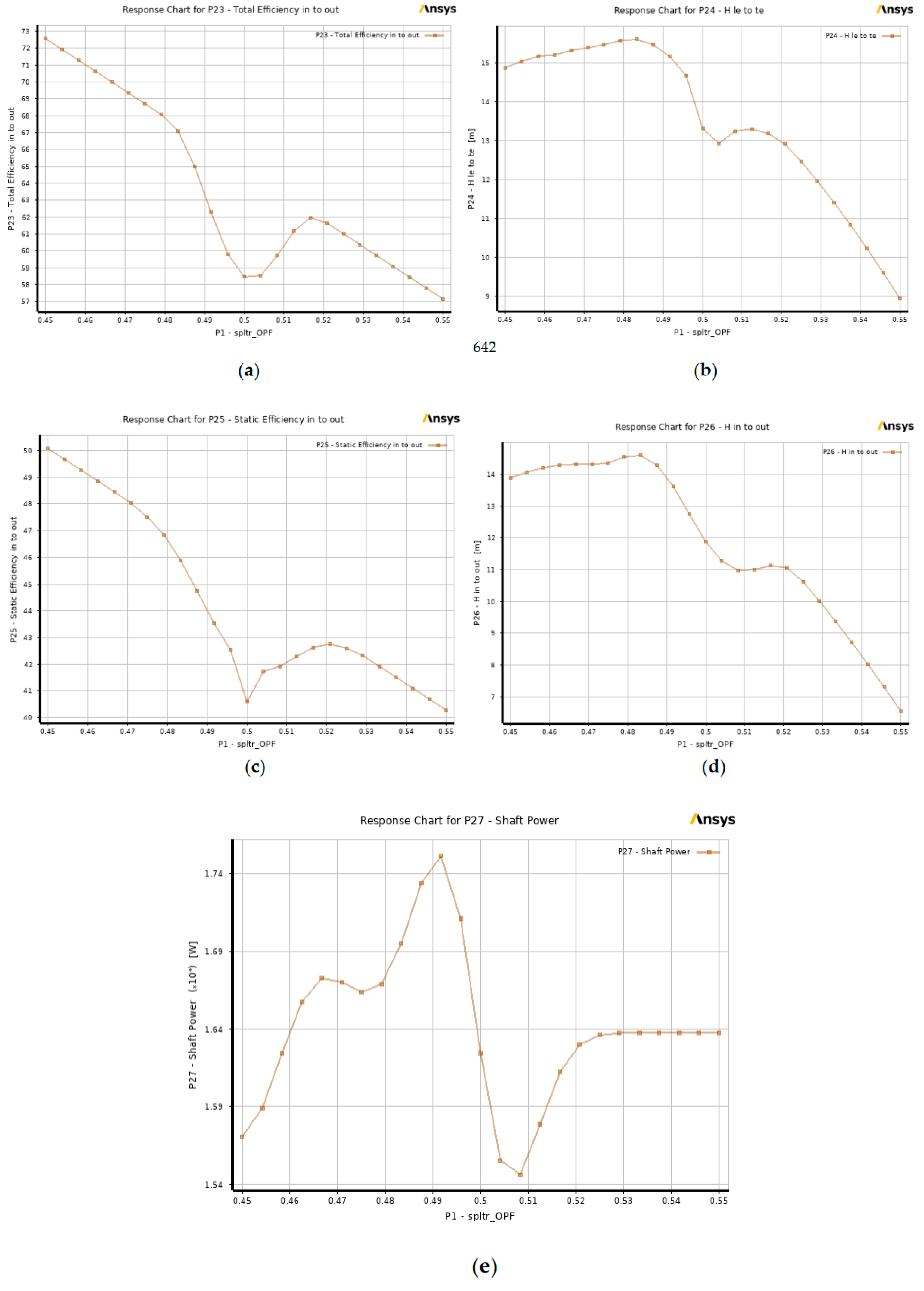
Figure 13.
The effect of volute tongue thickness and clearance in (a) total efficiency; (b) total head; (c) static efficiency; (d) static head; (e) shaft power.
Figure 13.
The effect of volute tongue thickness and clearance in (a) total efficiency; (b) total head; (c) static efficiency; (d) static head; (e) shaft power.
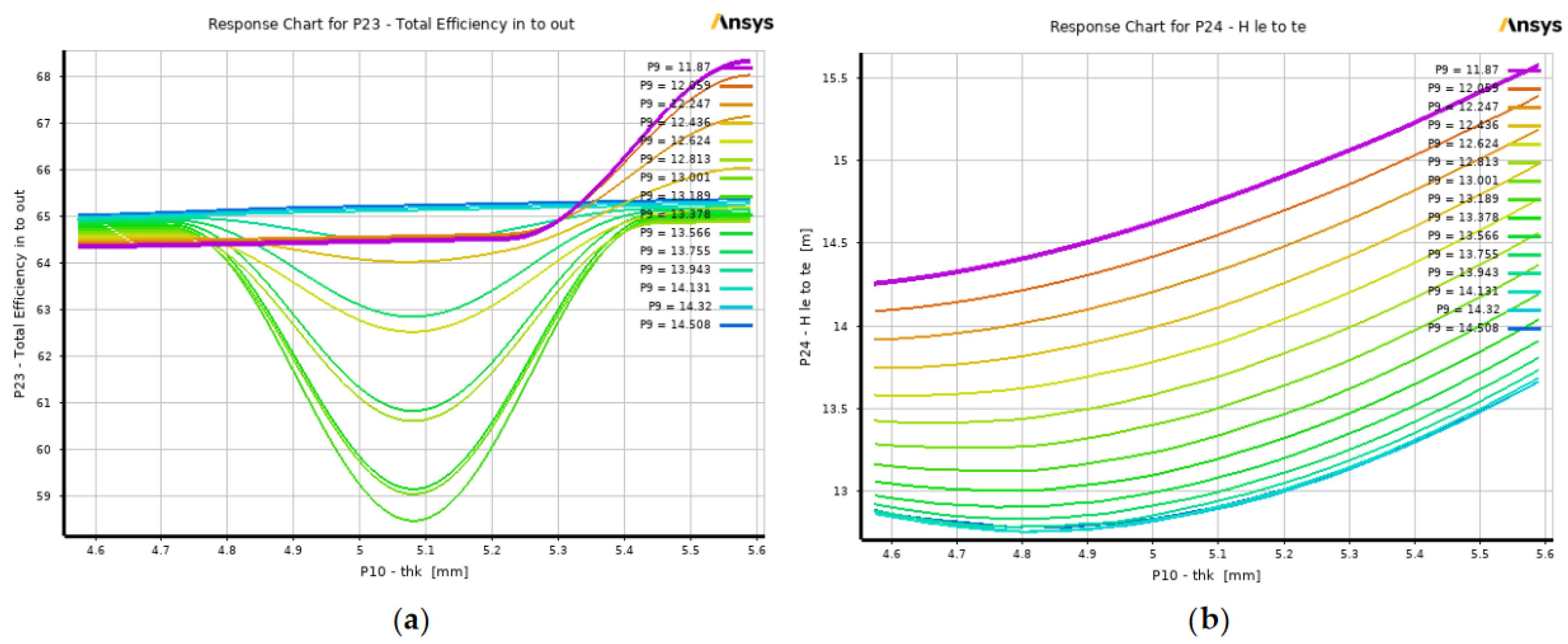
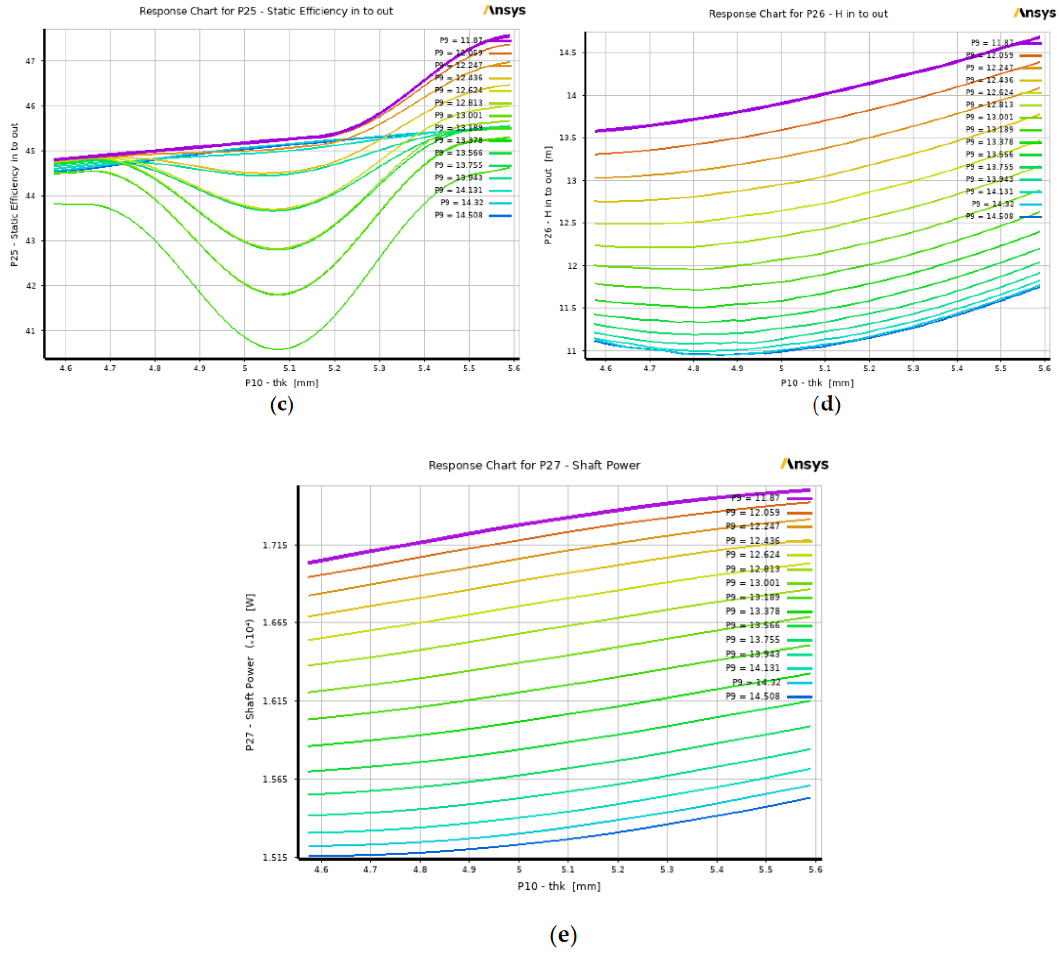
Figure 14.
The effect of varying (a) LE and (b) TE ellipse ratio in total efficiency.
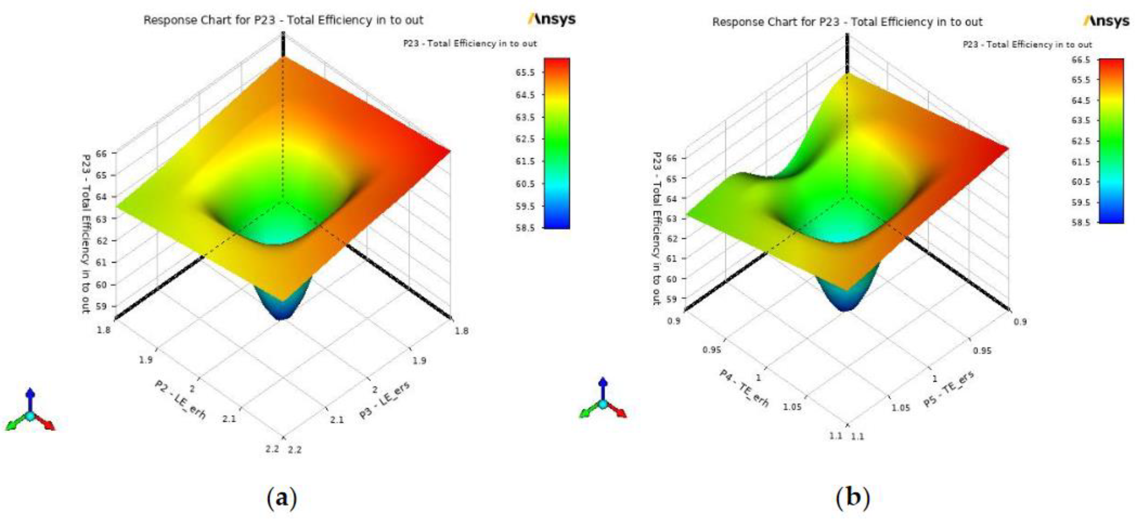
Figure 15.
The effect of varying (a) LE and (b) TE ellipse ratio in total head.
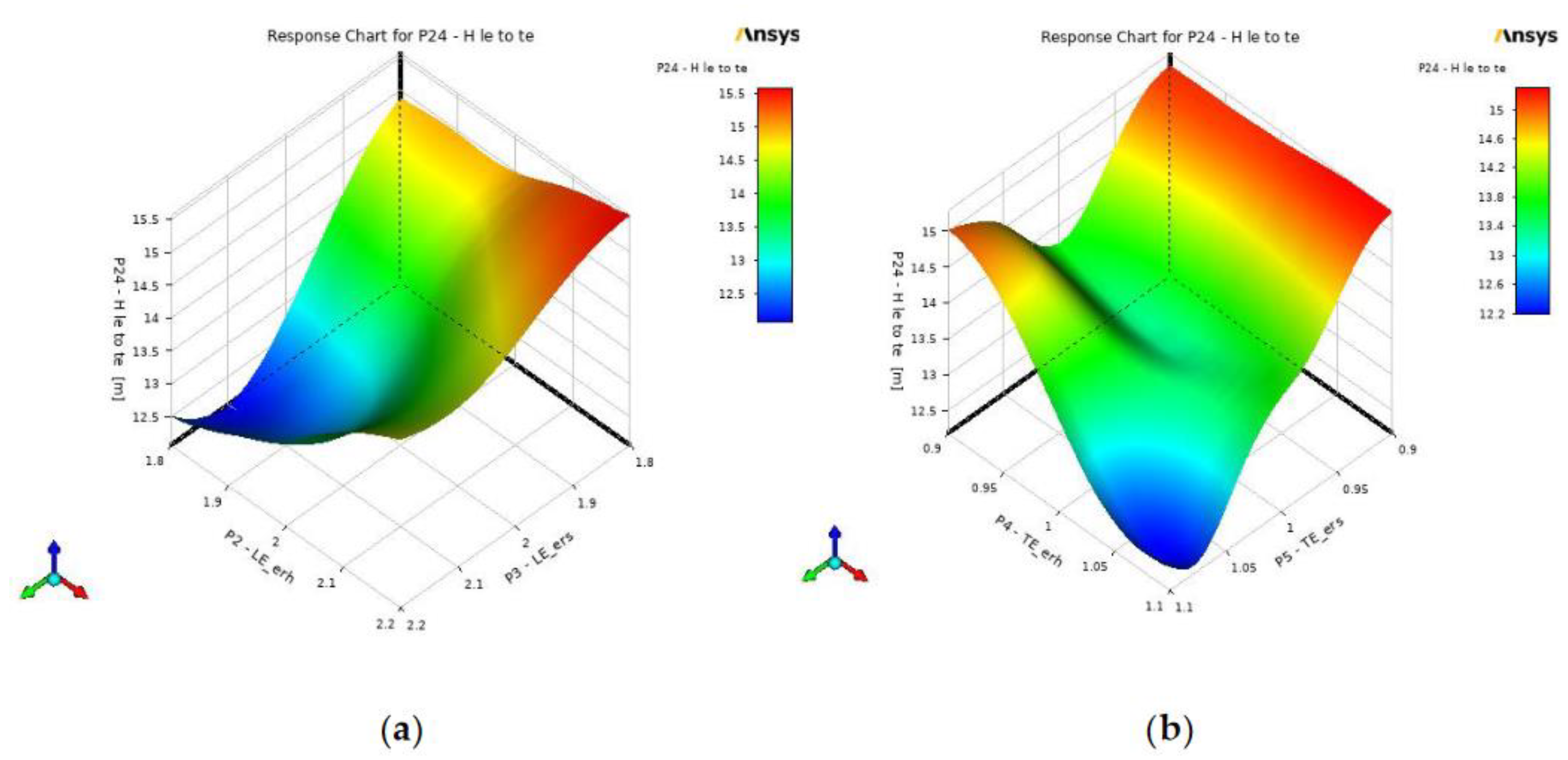
Figure 16.
The effect of varying (a) LE and (b) TE ellipse ratio in static efficiency.

Figure 17.
The effect of varying (a) LE and (b) TE ellipse ratio in static head.
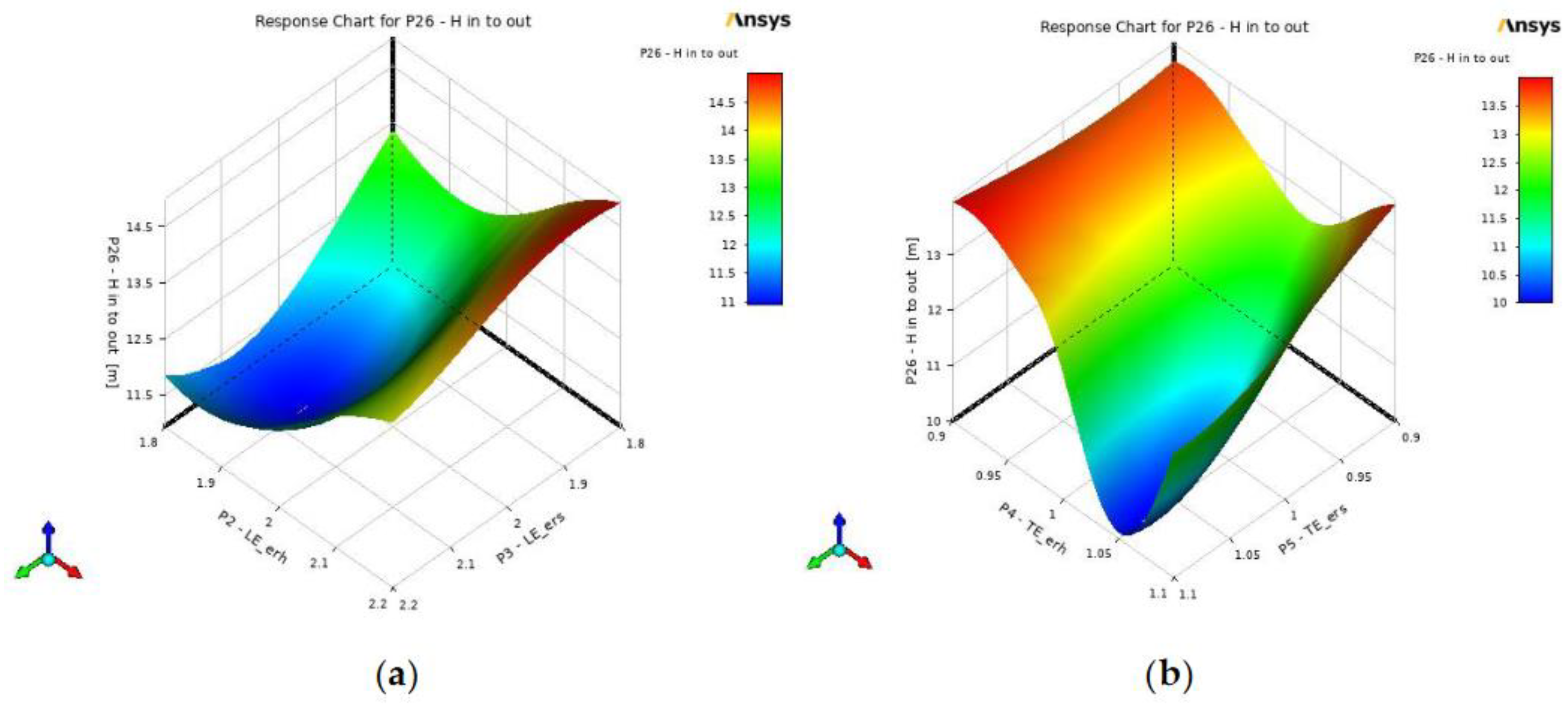
Figure 18.
The effect of varying (a) LE and (b) TE ellipse ratio in shaft power.
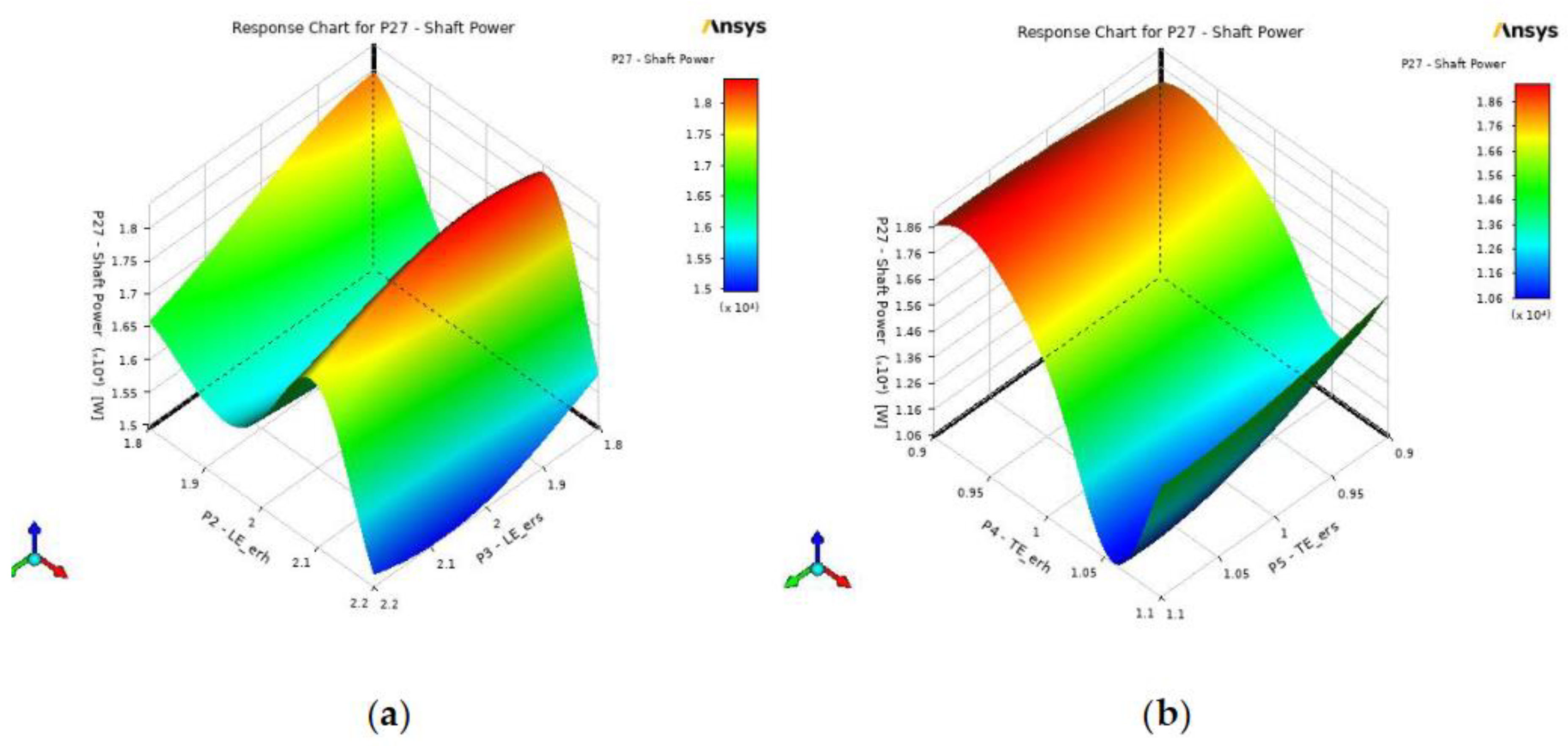
Figure 19.
The pressure contour plot of the (a) baseline design vs. (b) the optimized design.
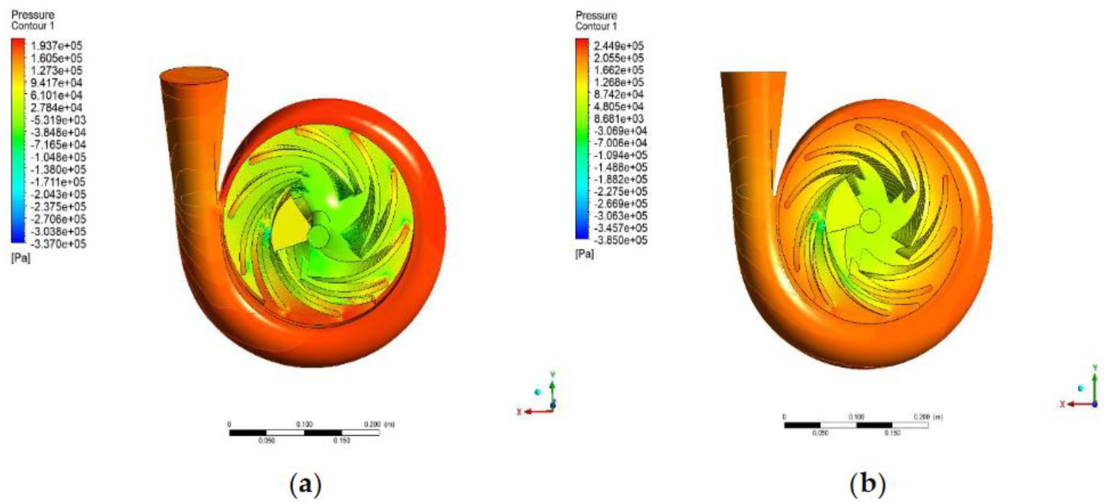
Figure 20.
The area-averaged pressure contour on the meridional surface of the (a) baseline design vs. (b) the optimized design.
Figure 20.
The area-averaged pressure contour on the meridional surface of the (a) baseline design vs. (b) the optimized design.
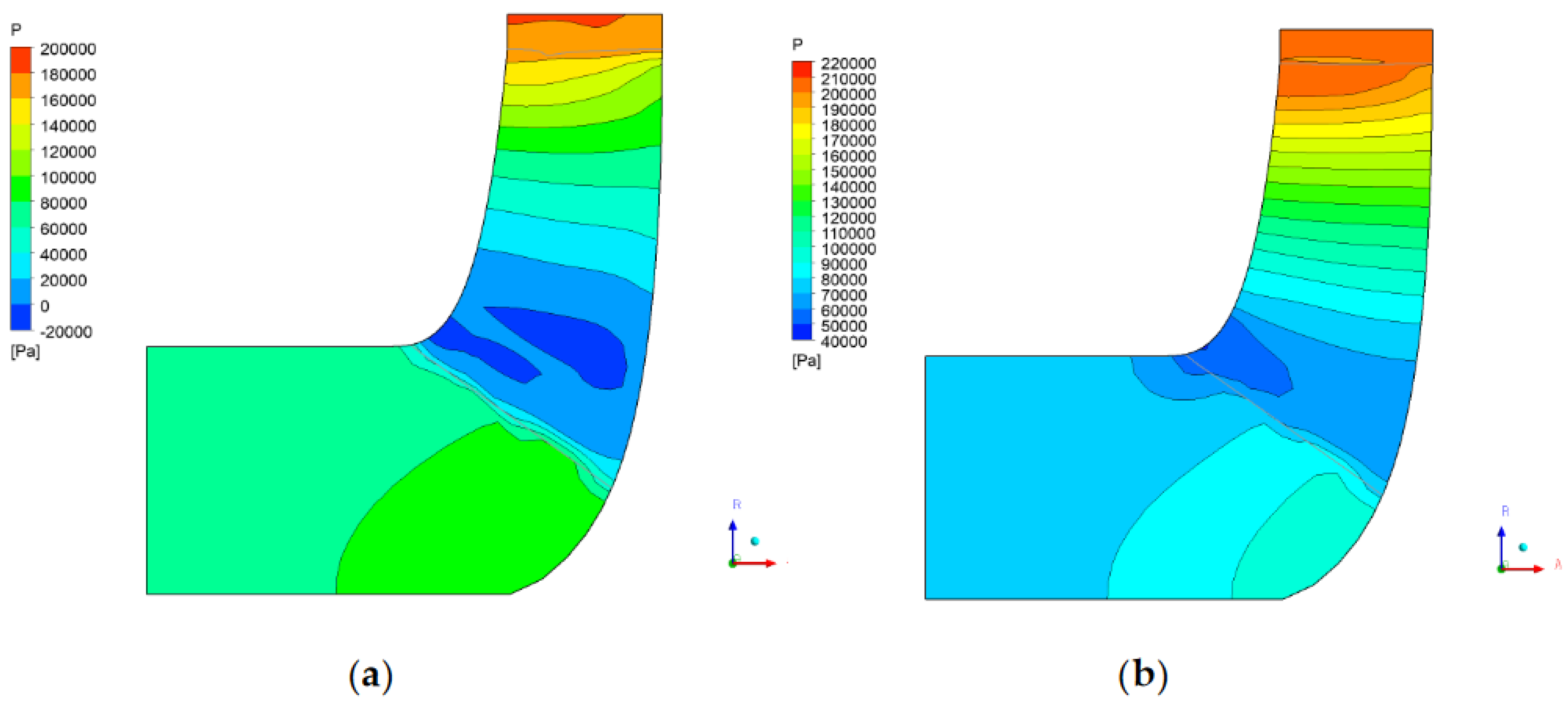
Figure 21.
The pressure cloud contour of the (a) baseline design vs. (b) the optimized design.
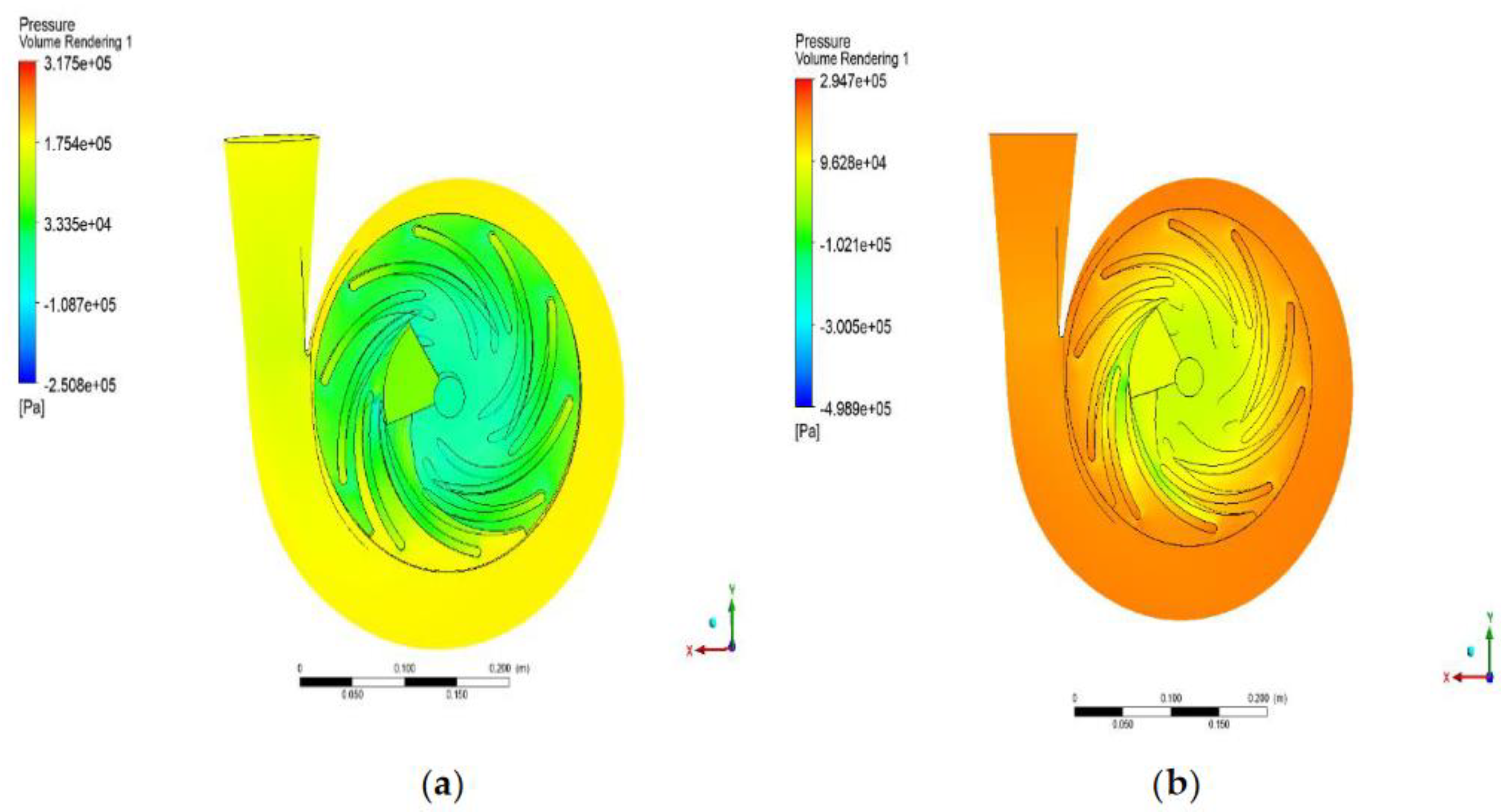
Figure 22.
The eddy viscosity cloud contour of the (a) baseline design vs. (b) the optimized design.
Figure 22.
The eddy viscosity cloud contour of the (a) baseline design vs. (b) the optimized design.
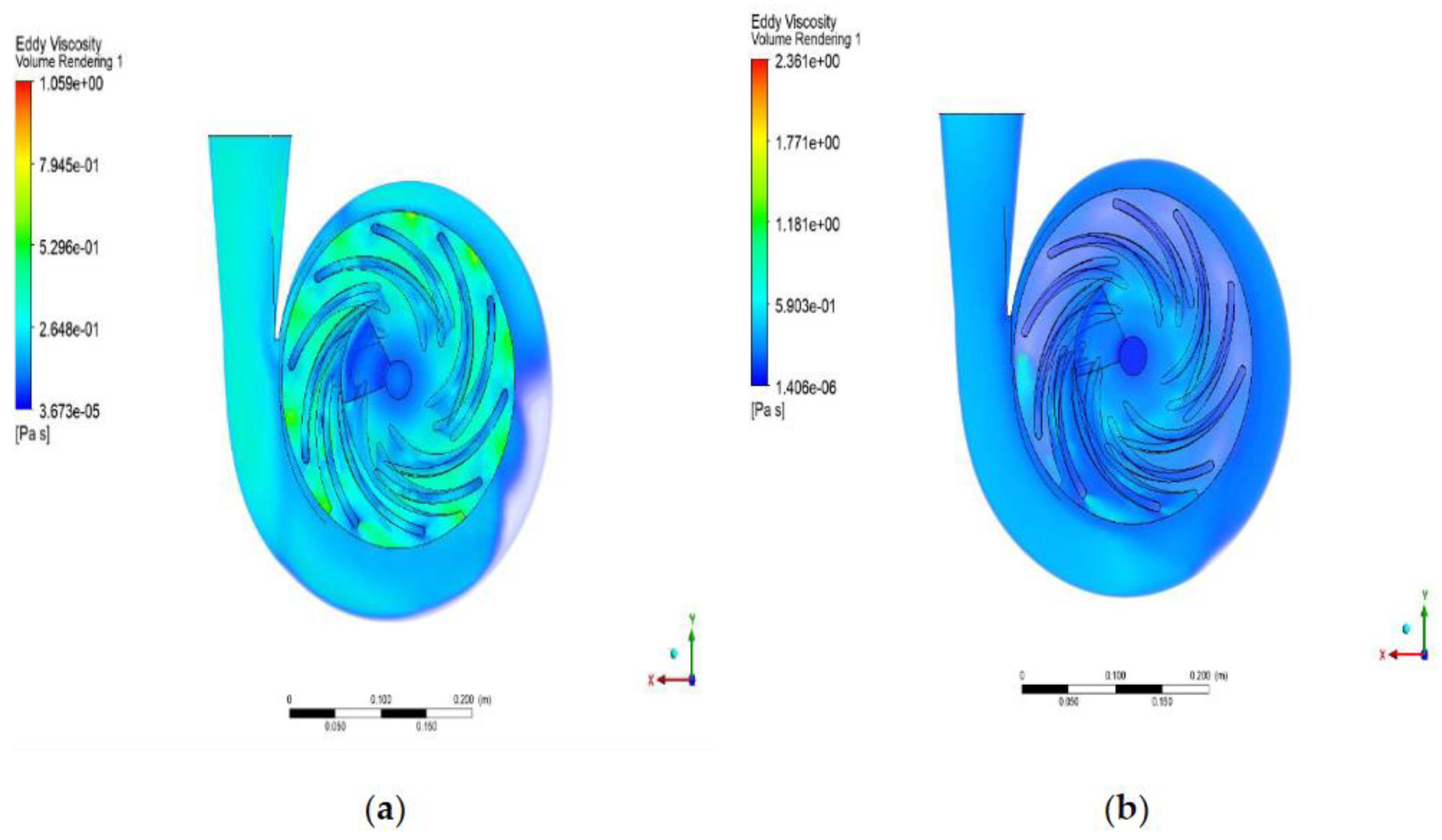
Figure 23.
The velocity streamline diagram of the (a) baseline design vs. (b) the optimized design.
Figure 24.
The overall velocity streamline diagram of the (a) baseline design vs. (b) the optimized design.
Figure 24.
The overall velocity streamline diagram of the (a) baseline design vs. (b) the optimized design.
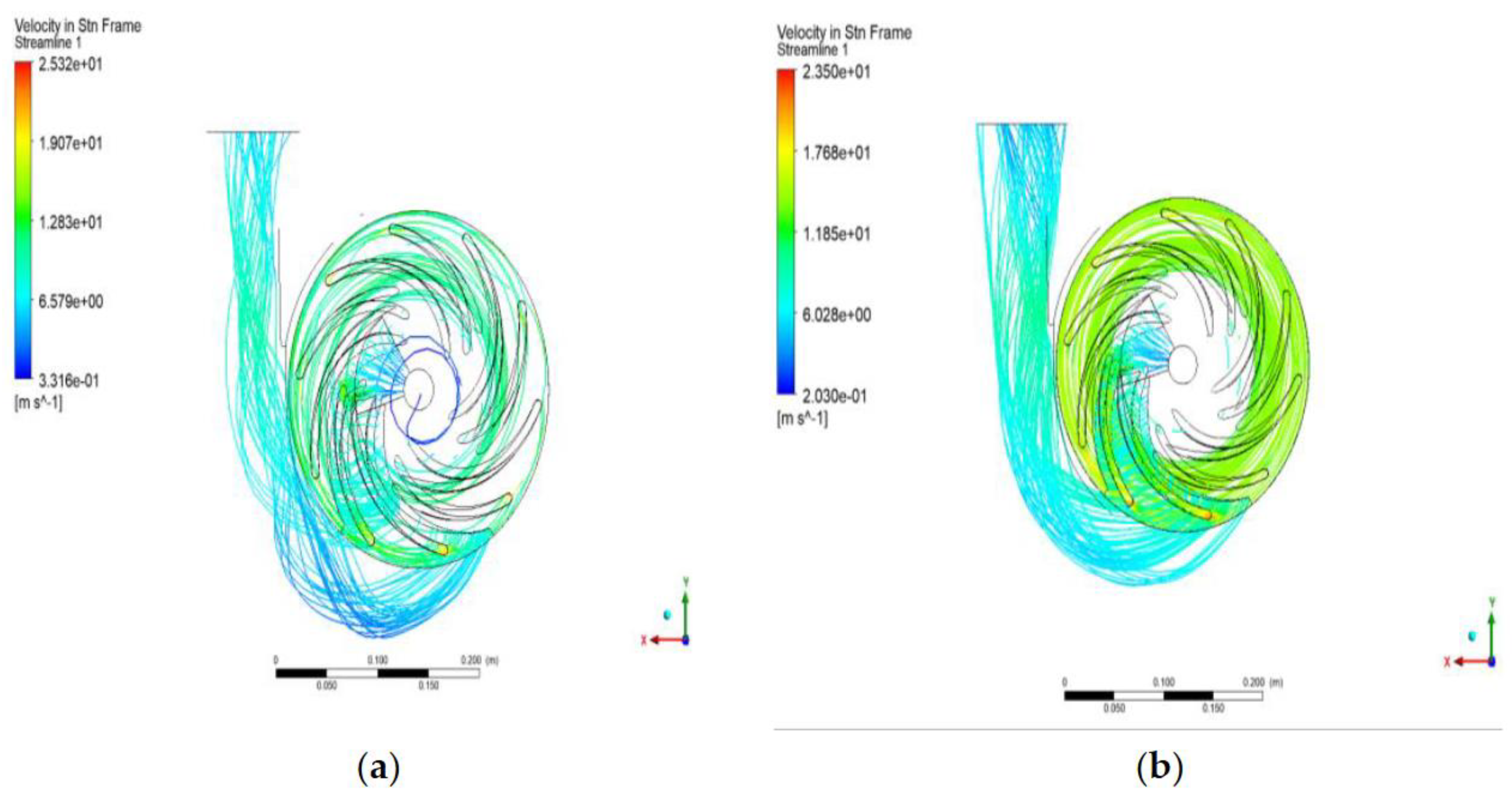

Table 1.
Vista CPD input parameters.
| Input Parameter | Unit | Value |
|---|---|---|
| Rotational Speed | RPM | 1600 |
| Volume Flow Rate | m3/hr | 120 |
| Density | kg/m3 | 1000 |
| Head Rise | m | 20 |
| Inlet Flow Angle | degrees | 90 |
| Merid Velocity Ratio | - | 1.1 |
| Number of Vanes | - | 5 |
Table 2.
Impeller specification.
| Impeller Specification | Unit | Value |
|---|---|---|
| Shaft Diameter | mm | 19.611 |
| Hub Eye Diameter | mm | 29.416 |
| Eye Diameter | mm | 125.75 |
| Vane Thickness | mm | 7.2602 |
| Tip Diameter | mm | 242.01 |
| Tip Width | mm | 30.215 |
| Number of Main Blade | - | 5 |
| Number of Splitter Blade | - | 5 |
Table 3.
Volute specification.
| Volute Specification | Unit | Value |
|---|---|---|
| Inlet Width | mm | 60.431 |
| Base Circle Radius | mm | 134.19 |
| Tongue Clearance | mm | 13.189 |
| Tongue Thickness | mm | 5.0821 |
| Diffuser Length | mm | 151.79 |
| Diffuser Cone Angle | degree | 7 |
| Diffuser Outlet Hydraulic Diameter | mm | 91.868 |
| Diffuser Outlet Height | mm | 91.868 |
Table 4.
Initial parameter values.
| Parameter | Unit | Value |
|---|---|---|
| Splitter Offset Pitch Fraction | - | 0.5 |
| TE Ellipse Ratio at Hub | - | 1 |
| TE Ellipse Ratio at Shroud | - | 1 |
| LE Ellipse Ratio at Hub | - | 2 |
| LE Ellipse Ratio at Shroud | - | 2 |
| Volute Tongue Thickness | mm | 5.0821 |
| Volute Tongue Clearance | mm | 13.198 |
Table 5.
Impeller and volute mesh details.
| Mesh Details | Impeller | Volute |
|---|---|---|
| Element Size (mm) | 19.106 | 7.0216 |
| Growth Rate | 1.2 | 1.3 |
| Max Size (mm) | 38.213 | 14.043 |
| Defeature Size (mm) | 0.095532 | 0.035108 |
| Curvature Minimum Size | 0.19106 | 0.070216 |
| Curvature Normal Angle (°) | 18 | 30 |
| Bounding Box Diagonal (mm) | 382.13 | 535.75 |
| Average Surface Area (mm) | 2.2651 | 7.9889 |
| Minimum Edge Length (mm) | 0.029689 | 0.23622 |
| Target Skewness | 0.9 | 0.9 |
| Maximum Layers | 5 | 5 |
| Pinch Tolerance (mm) | 0.17196 | 0.063194 |
| Nodes | 157,966 | 75,273 |
| Elements | 795,202 | 212,845 |
Table 6.
Total mesh elements and nodes of the design.
| Details | Nodes | Elements |
|---|---|---|
| Impeller | 157,966 | 795,202 |
| Volute | 75,273 | 212,845 |
| Total | 233,239 | 1,008,047 |
Table 7.
Defined properties of water.
| Data | Unit | Value |
|---|---|---|
| Density | kg/m3 | 997 |
| Specific Heat Capacity | J/kg-K | 4181.7 |
| Reference Temperature | °C | 25 |
| Reference Pressure | atm | 1 |
| Dynamic Viscosity | kg/m-s |
Table 8.
CFD simulation results of the centrifugal pump baseline model.
| Data | Unit | Value |
|---|---|---|
| Total Efficiency | % | 58.458 |
| Total Head | m | 13.041 |
| Static Efficiency | % | 40.592 |
| Static Head | m | 11.621 |
| Shaft Power | W | 16,246 |
Table 9.
DOE-generated design points.
| DP | spltr_ OPF |
LE_ erh |
LE_ ers |
TE_ erh |
TE_ ers |
clear (mm) |
thk (mm) |
(%) |
(m) |
(%) |
(m) |
SP (W) |
|---|---|---|---|---|---|---|---|---|---|---|---|---|
| 1 | 0.5 | 2 | 2 | 1 | 1 | 13.189 | 5.0821 | 58.458 | 13.041 | 40.592 | 11.621 | 16246 |
| 2 | 0.46723 | 2.1951 | 2.1746 | 1.0769 | 1.0985 | 14.494 | 5.5856 | 70.981 | 15.859 | 48.823 | 14.561 | 16765 |
| 3 | 0.45302 | 1.8136 | 1.8328 | 1.0966 | 0.92146 | 12.138 | 4.6592 | 71.93 | 15.325 | 49.818 | 14.184 | 16115 |
| 4 | 0.45373 | 1.825 | 2.1757 | 0.90945 | 1.0981 | 13.994 | 5.5237 | 72.258 | 15.215 | 49.974 | 14.05 | 15891 |
| 5 | 0.45521 | 2.1873 | 2.1907 | 1.0926 | 0.92327 | 12.441 | 5.5748 | 71.472 | 15.138 | 49.448 | 14.025 | 16036 |
| 6 | 0.46296 | 1.8211 | 2.181 | 0.90726 | 0.91337 | 14.387 | 4.8003 | 70.921 | 15.564 | 48.979 | 14.382 | 16572 |
| 7 | 0.46263 | 2.088 | 2.1487 | 0.90191 | 1.0999 | 11.956 | 4.6413 | 69.693 | 15.144 | 47.945 | 13.876 | 16271 |
| 8 | 0.45215 | 2.133 | 1.8968 | 1.0878 | 0.91123 | 14.471 | 4.6461 | 72.357 | 14.243 | 50.098 | 13.089 | 14783 |
| 9 | 0.45631 | 2.1861 | 1.8099 | 0.92996 | 0.93931 | 12.19 | 5.5574 | 69.367 | 13.818 | 48.152 | 12.565 | 14804 |
| 10 | 0.45114 | 2.197 | 1.9524 | 1.0996 | 1.0969 | 13.016 | 4.6227 | 70.804 | 14.638 | 48.46 | 13.528 | 15614 |
| 11 | 0.45827 | 1.8329 | 1.8578 | 0.96812 | 1.0987 | 14.432 | 4.6329 | 73.68 | 15.29 | 50.106 | 14.024 | 15555 |
| 12 | 0.46284 | 1.8121 | 1.807 | 0.90044 | 1.0545 | 11.951 | 5.2371 | 69.92 | 14.362 | 47.593 | 13.077 | 15284 |
| 13 | 0.46384 | 2.1256 | 2.0838 | 0.90369 | 0.91826 | 14.42 | 5.5878 | 69.84 | 15.726 | 48.57 | 14.56 | 17037 |
| 14 | 0.45873 | 1.8102 | 1.8412 | 1.0938 | 0.92137 | 14.189 | 5.3898 | 69.62 | 15.269 | 48.187 | 14.104 | 16556 |
| 15 | 0.46126 | 2.042 | 1.8139 | 0.90462 | 0.90982 | 12.35 | 4.5835 | 69.73 | 14.848 | 47.904 | 13.637 | 15982 |
Table 10.
Indicated response surface tolerances.
| Data | Unit | Value |
|---|---|---|
| Total Efficiency | % | 1 |
| Total Head | m | 0.5 |
| Static Efficiency | % | 1 |
| Static Head | m | 0.5 |
| Shaft Power | W | 0.5 |
Table 11.
Objectives and constraints of the optimization study.
| Data | Objectives | Constraints | |
|---|---|---|---|
| Type | Target | ||
| Total Efficiency | Maximize | 85 | ≥ 70% |
| Total Head | Maximize | 16 | ≥ 12 m |
| Static Efficiency | Maximize | 60 | ≥ 40% |
| Static Head | Maximize | 13 | ≥ 10 m |
| Shaft Power | Minimize | 15000 | ≥ 10,000 W |
Table 12.
Comparison of total efficiency and head from related study and CFD simulation.
| Parameter | Experimental | CFD | Percent Difference (%) |
|---|---|---|---|
| Total Efficiency (%) | 59.03 | 58.458 | 0.97372 |
| Shaft Power (m) | 13.00 | 13.041 | 0.31489 |
Table 13.
Generated minimum and maximum response.
| Parameter | Minimum | Maximum |
|---|---|---|
| Total Efficiency (%) | 53.527 | 86.262 |
| Total Head (m) | 6.9756 | 18.383 |
| Static Efficiency (%) | 33.893 | 58.479 |
| Static Head (m) | 4.9608 | 17.401 |
| Shaft Power (W) | 4936.6 | 20954 |
Table 14.
Optimal input design parameters of the study.
| Input Parameter | Candidate Point 1 | Candidate Point 2 | Candidate Point 3 |
|---|---|---|---|
| Spltr_OPF | 0.45011 | 0.45022 | 0.45011 |
| LE_erh | 2.1101 | 2.0947 | 2.0919 |
| LE_ers | 1.8104 | 1.816 | 1.8194 |
| TE_erh | 1.0148 | 1.0123 | 1.0141 |
| TE_ers | 0.90063 | 0.90073 | 0.90115 |
| clear (mm) | 12.994 | 12.888 | 12.772 |
| thk (mm) | 5.5787 | 5.5887 | 5.584 |
Table 15.
Optimal design output results of the study.
| Output Parameter | Candidate Point 1 | Candidate Point 2 | Candidate Point 3 |
|---|---|---|---|
| Total Efficiency (%) | 74.445 | 74.315 | 74.293 |
| Total Head (m) | 15.088 | 15.107 | 15.095 |
| Static Efficiency (%) | 52.029 | 51.972 | 51.971 |
| Static Head (m) | 13.558 | 13.59 | 13.573 |
| Shat Power (W) | 14888 | 14914 | 14891 |
Table 16.
Comparison of results for baseline and optimized design.
| Input Parameter | Baseline Design | Optimized Design | Percentage Improvement (%) |
|---|---|---|---|
| spltr_OPF | 0.5 | 0.45011 | - |
| LE_erh | 2 | 2.1101 | - |
| LE_ers | 2 | 1.8104 | - |
| TE_erh | 1 | 1.0148 | - |
| TE_ers | 1 | 0.90063 | - |
| clear (mm) | 13.189 | 12.994 | - |
| thk (mm) | 5.0821 | 5.5787 | - |
| Output Parameter | |||
| Total Efficiency (%) | 58.458 | 74.445 | 27.35 |
| Total Head (m) | 13.041 | 15.088 | 15.70 |
| Static Efficiency (%) | 40.592 | 52.029 | 28.18 |
| Static Head (m) | 11.621 | 13.558 | 16.67 |
| Shaft Power (W) | 16246 | 14888 | 8.36 |
Disclaimer/Publisher’s Note: The statements, opinions and data contained in all publications are solely those of the individual author(s) and contributor(s) and not of MDPI and/or the editor(s). MDPI and/or the editor(s) disclaim responsibility for any injury to people or property resulting from any ideas, methods, instructions or products referred to in the content. |
© 2024 by the authors. Licensee MDPI, Basel, Switzerland. This article is an open access article distributed under the terms and conditions of the Creative Commons Attribution (CC BY) license (http://creativecommons.org/licenses/by/4.0/).
Copyright: This open access article is published under a Creative Commons CC BY 4.0 license, which permit the free download, distribution, and reuse, provided that the author and preprint are cited in any reuse.


