Submitted:
08 November 2024
Posted:
08 November 2024
You are already at the latest version
Abstract
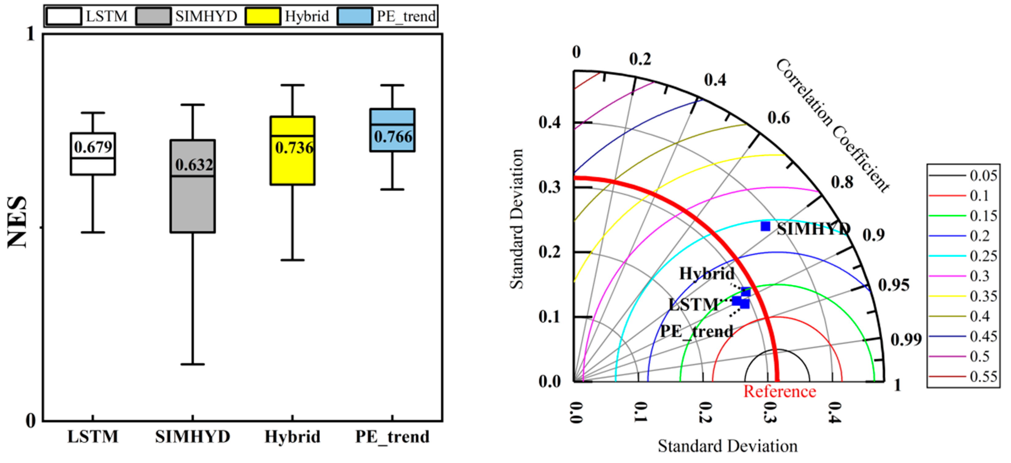
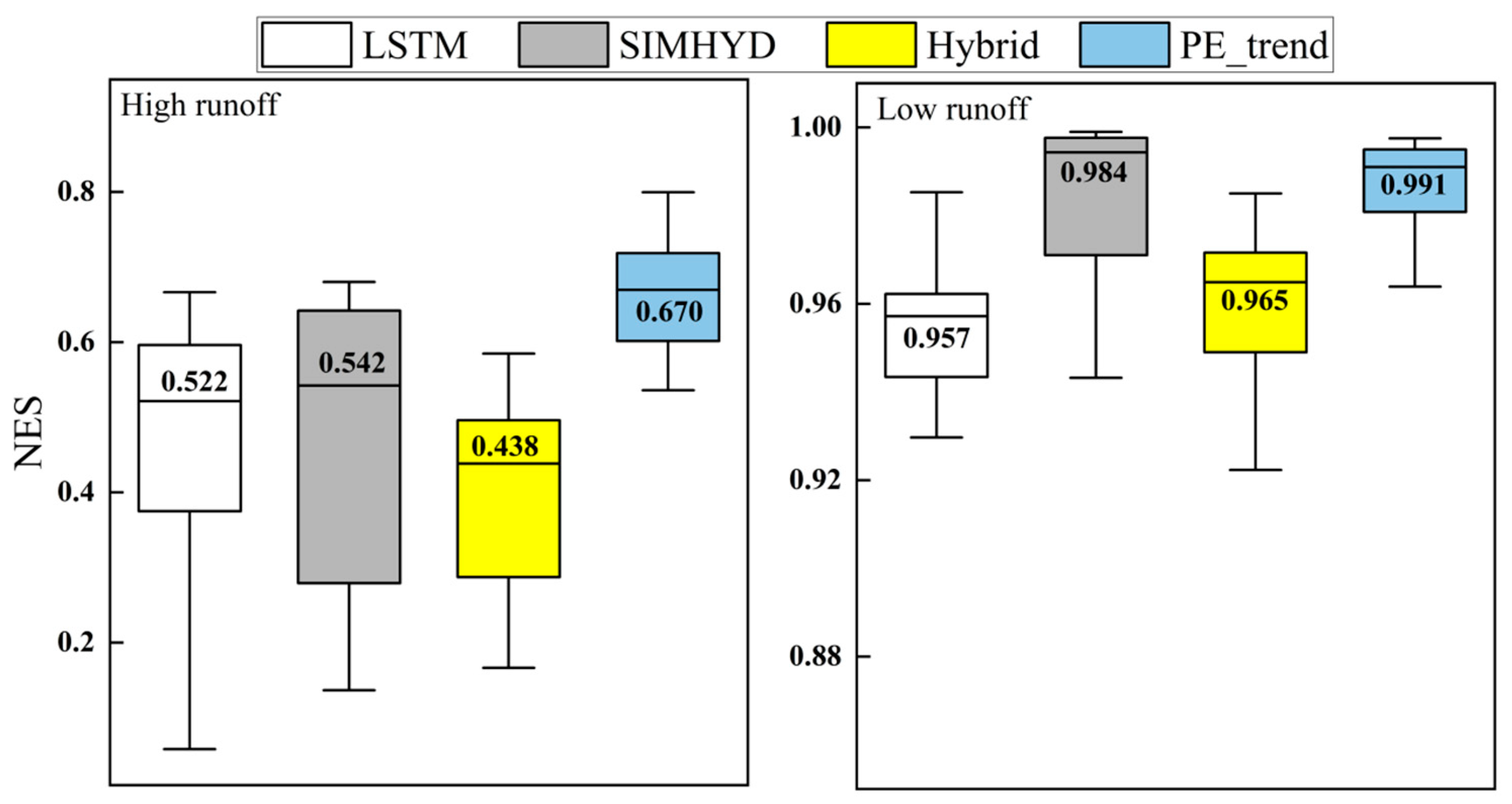
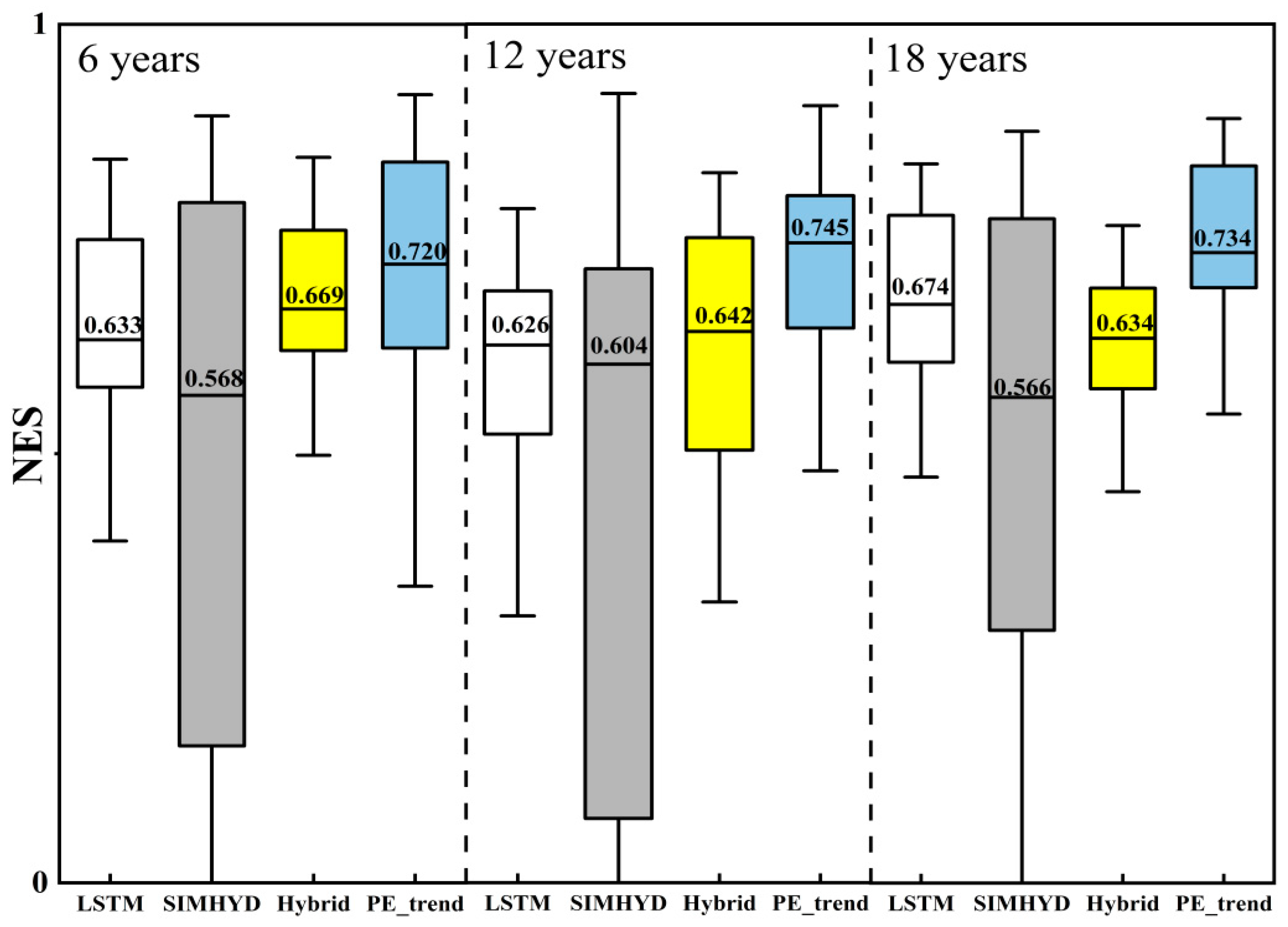
The inherent uncertainties in traditional hydrological models present significant chal-lenges for accurately simulating runoff. Combining machine learning models with tradi-tional hydrological models is an essential approach to enhancing the runoff modeling capabilities of hydrological models. However, research on the impact of mixed models on runoff simulation capability is limited. Therefore, this study uses the traditional hy-drological model SIMHYD and the machine learning model LSTM (Long Short-Term Memory) to construct two coupled models: a direct coupling model and a dynamically improved predictive validity hybrid model. These models were evaluated using the US CAMELS dataset to assess the impact of the two model combination methods on runoff modeling capabilities. The results indicate that the runoff modeling capabilities of both model combination methods were improved compared to individual models, with the dynamically improved predictive validity hybrid model demonstrating the optimal mod-eling capability. Compared to LSTM, this hybrid model showed a 12.8% increase in the Nash-Sutcliffe efficiency (NSE) median value for daily runoff during the validation pe-riod, a 28.4% increase in the NSE median value for high flows compared to SIMHYD, this hybrid model showed a 12.5% increase in the NSE median value for daily runoff during the validation period, a 23.6% increase in the NSE median value for high flows, and a significant improvement in the stability of low-flow runoff simulations. In per-formance testing involving varying training period lengths, the PE_trend model trained for 12 years exhibited the best performance, showing a 3.5% and 1.5% increase in the median NES compared to training periods of 6 years and 18 years, respectively.
Keywords:
1. Introduction
2. Materials and Methods
2.1. Research Area and Data
2.2. Models and Methods
2.2.1. Introduction to Hydrological Models
2.2.2. Introduction to LSTM Model
2.2.3. Combined Model Hybrid
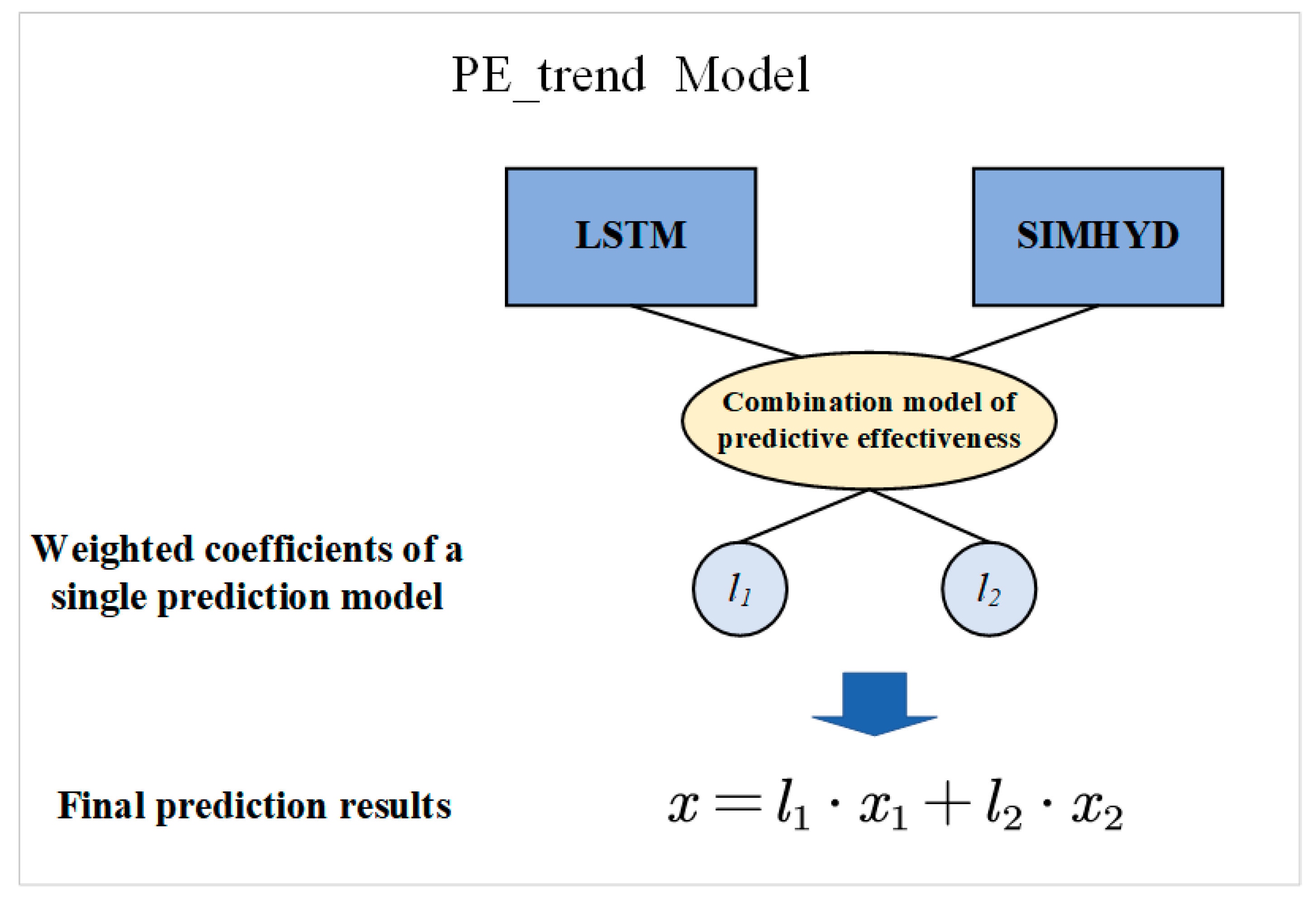
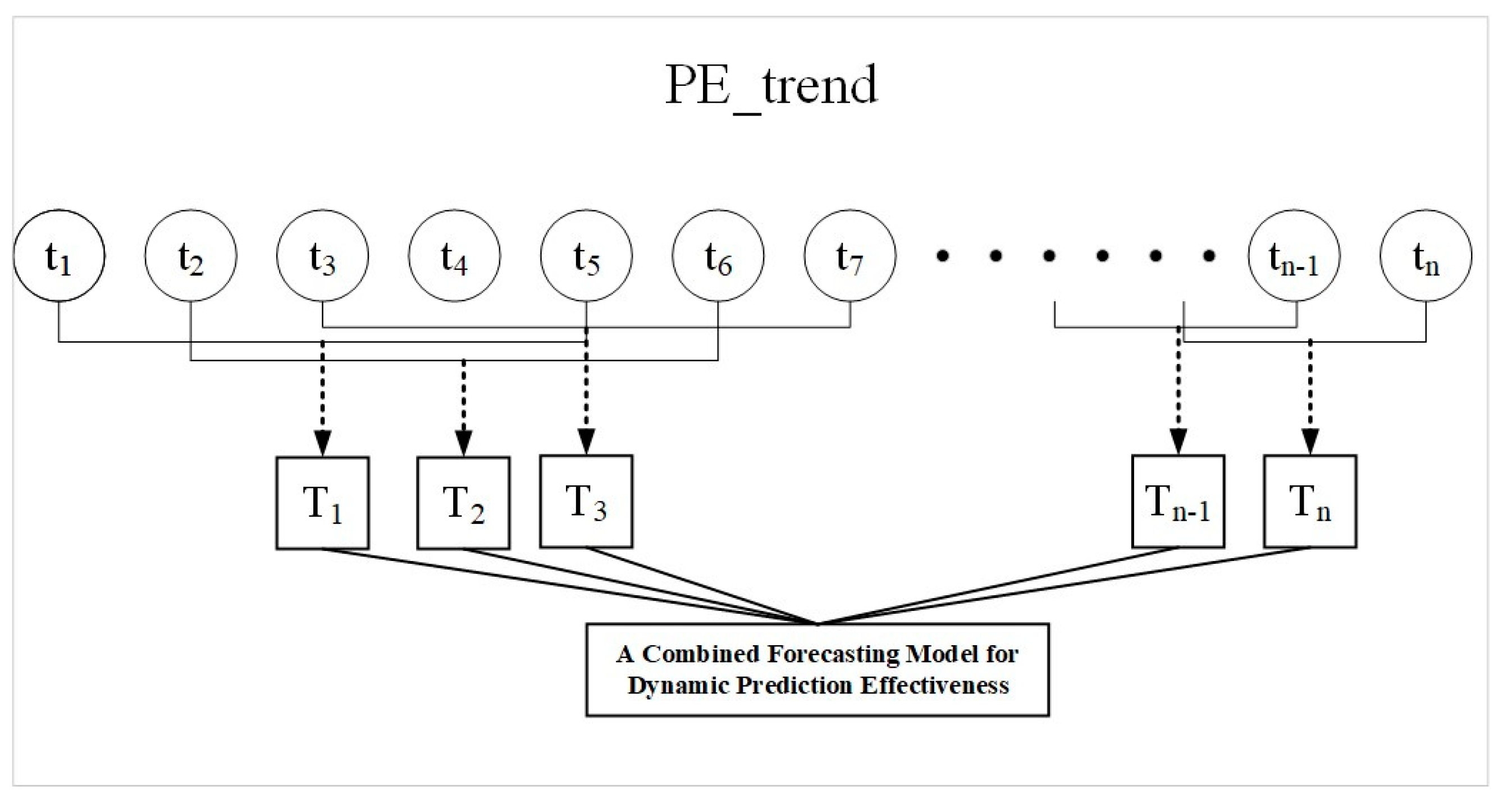
2.2.4. Hybrid Model PE_Trend Based on Dynamic Prediction Effectiveness


2.2.5. Model Evaluation Indicators


3. Results
3.1. Model Runoff Simulation Capability
3.2. The Ability of the Model to Simulate Extreme Traffic
4. Discussion
4.1. The Predictive Performance of the Model Under Different Training Periods of Length
4.2. The Runoff Simulation Ability of Individual and Combined Models
4.3. Limitations and Future Challenges
5. Conclusion
Author Contributions
Funding
Data Availability Statement
Conflicts of Interest
References
- Doycheva K, Horn G, Koch C, et al. Assessment and weighting of meteorolog-ical ensemble forecast members based on supervised machine learning with appli-cation to runoff simulations and flood warning[J]. Advanced Engineering Infor-matics, 2017, 33: 427–439.
- Kreibich H, Thieken A H, Petrow T, et al. Flood loss reduction of private households due to building precautionary measures–lessons learned from the Elbe flood in 02[J]. Natural hazards and earth system sciences, 2005, 5(1): 117-126. 20 August.
- Blöschl G, Sivapalan M. Scale issues in hydrological modelling: a review[J]. Hy-drological Processes, 1995, 9(3-4): 251-290.
- Wang X, Liu T, Yang W. Development of a robust runoff-prediction model by fusing the rational equation and a modified SCS-CN method[J]. Hydrological Sci-ences Jour-nal, 2012, 57(6): 1118–1140.
- Gebregiorgis A S, Hossain F. Understanding the dependence of satellite rainfall un-certainty on topography and climate for hydrologic model simulation[J]. IEEE Transac-tions on Geoscience and Remote Sensing, 2012, 51(1): 704–718.
- Burges S, J. Streamflow prediction: capabilities, opportunities, and challenges[J]. Hydrologic Sciences: Taking Stock and Looking Ahead, 1998, 5: 101–134.
- Talei A, Chua L H C. Influence of lag time on event-based rainfall–runoff mod-eling using the data driven approach[J]. Journal of Hydrology, 2012, 438: 223–233.
- Xiao W, Zhou J, Yang J, et al. Long-term runoff forecast in the middle and low-er reaches of the Yangtze River based on machine learning[J]. Water Resources and Power, 2022, 40(09): 31-34+26. [CrossRef]
- Nayak P C, Venkatesh B, Krishna B, et al. Rainfall-runoff modeling using con-ceptual, data-driven, and wavelet-based computing approaches [J]. Journal of Hy-drology, 2013, 493: 57–67.
- Chang C W, Dinh N T. Classification of machine learning frameworks for da-ta-driven thermal fluid models[J]. International Journal of Thermal Sciences, 2019, 135: 559–579.
- Gharari S, Razavi S. A review and synthesis of hysteresis in hydrology and hydro-logical modeling: Memory, path-dependency, or missing physics?[J]. Journal of Hy-drology, 2018, 566: 500–519.
- Noble W, S. What is a support vector machine?[J]. Nature Biotechnology, 2006, 24(12): 1565–1567.
- Rigatti S, J. Random forest[J]. Journal of Insurance Medicine, 2017, 47(1): 31-39.
- Yin C, Zhu Y, Fei J, et al. A deep learning approach for intrusion detection us-ing recurrent neural networks[J]. Ieee Access, 2017, 5: 21954–21961.
- Yang Y, McVicar T R, Donohue R J, et al. Lags in hydrologic recovery fol-lowing an extreme drought: Assessing the roles of climate and catchment charac-teristics[J]. Water Resources Research, 2017, 53(6): 4821–4837.
- Siami-Namini S, Namin A S. Forecasting economics and financial time series: ARIMA vs. LSTM[J]. arXiv:1803.06386, 2018.
- Amalou I, Mouhni N, Abdali A. Multivariate time series prediction by RNN archi-tectures for energy consumption forecasting[J]. Energy Reports, 2022, 8: 1084–1091.
- Man Y, Yang Q, Shao J, et al. Enhanced LSTM model for daily runoff predic-tion in the upper Huai river basin, China[J]. Engineering, 2022.
- Kanai S, Fujiwara Y, Iwamura S. Preventing gradient explosions in gated re-current units[J]. Advances in neural information processing systems, 2017, 30.
- Hochreiter S, Schmidhuber J. Long short-term memory[J]. Neural Computa-tion, 1997, 9(8): 1735-1780.
- Kim C, Kim C S. Comparison of the performance of a hydrologic model and a deep learning technique for rainfall-runoff analysis[J]. Tropical Cyclone Research and Review, 2021, 10(4): 215–222.
- Yuan X, Chen C, Lei X, et al. Monthly runoff forecasting based on LSTM–ALO model[J]. Stochastic environmental research and risk assessment, 2018, 32: 2199-2212.
- Adnan R M, Dai H L, Mostafa R R, et al. Modeling multistep ahead dissolved ox-ygen concentration using improved support vector machines by a hybrid me-taheuristic algorithm[J]. Sustainability, 2022, 14(6): 3470.
- [24]Adnan R M, Mostafa R R, Dai H L, et al. Pan evaporation estimation by rele-vance vector machine tuned with new metaheuristic algorithms using limited cli-matic data[J]. Engineering Applications of Computational Fluid Mechanics, 2023, 17(1): 2192258.
- Okkan U, Ersoy Z B, Kumanlioglu A A, et al. Embedding machine learning tech-niques into a conceptual model to improve monthly runoff simulation: A nested hybrid rainfall-runoff modeling[J]. Journal of Hydrology, 2021, 598: 126433.
- Liu J, Yuan X, Zeng J, et al. Ensemble streamflow forecasting over a cascade res-ervoir catchment with integrated hydrometeorological modeling and machine learn-ing[J]. Hydrology and Earth System Sciences, 2022, 26(2): 265-278.
- Yang S, Yang D, Chen J, et al. A physical process and machine learning com-bined hydrological model for daily streamflow simulations of large watersheds with limited observation data[J]. Journal of Hydrology, 2020, 590: 125206.
- Liu Q, Ma X, Yan S, et al. Lag in hydrologic recovery following extreme me-teorological drought events: implications for ecological water requirements[J]. Wa-ter, 2020, 12(3): 837.
- Yu Q, Jiang L, Wang Y, et al. Enhancing streamflow simulation using hybrid-ized machine learning models in a semiarid basin of the Chinese loess Plateau[J]. Journal of Hydrology, 2023, 617: 129115.
- Bai P, Liu X, Yang T, et al. Assessment of the influences of different potential evapotranspiration inputs on the performance of monthly hydrological models un-der different climatic conditions[J]. Journal of Hydrometeorology, 2016, 17(8): 2259-2274.
- Chiew F H S, Peel M C, Western A W. Application and testing of the simple rain-fall-runoff model SIMHYD[J]. Mathematical models of small watershed hy-drology and applications, 2002: 335–367.
- A: Bai, Xiaomang Liu, Jiaxin Xie, Simulating runoff under changing cli-matic conditions, 2021. [CrossRef]
- Lin F, Chen X, Yao H. Evaluating the use of Nash-Sutcliffe efficiency coeffi-cient in goodness-of-fit measures for daily runoff simulation with SWAT[J]. Journal of Hy-drologic Engineering, 2017, 22(11): 05017023.
- Michaud J, Sorooshian S. Comparison of simple versus complex distributed runoff models on a midsized semiarid watershed[J]. Water resources research, 1994, 30(3): 593–605.
- Elshorbagy A, Simonovic S P, Panu U S. Performance evaluation of artificial neural networks for runoff prediction[J]. Journal of Hydrologic Engineering, 2000, 5(4): 424–427.
- Piotrowski A P, Napiorkowski J J. A comparison of methods to avoid overfit-ting in neural networks training in the case of catchment runoff modeling [J]. Jour-nal of Hy-drology, 2013, 476: 97–111.
- Hong J, Wang Z, Yao Y. Fault prognosis of battery system based on accurate volt-age abnormity prognosis using long short-term memory neural networks[J]. Applied Energy, 2019, 251: 113381.
- Gu J, Zheng Z, Lan Z, et al. Dynamic meta-learning for failure prediction in large-scale systems: A case study[C]//2008 37th International Conference on Paral-lel Processing. IEEE, 2008: 157-164.
- Zheng Q, Yang M, Yang J, et al. Improvement of generalization ability of deep CNN via implicit regularization in two-stage training process[J]. IEEE Access, 2018, 6: 15844-15869.
- Zhang G P, Qi M. Neural network forecasting for seasonal and trend time se-ries[J]. European journal of operational research, 2005, 160(2): 501–514.
- Mohammadi B, Safari M J S, Vazifehkhah S. IHACRES, GR4J and MISD-based multi conceptual-machine learning approach for rainfall-runoff mod-eling[J]. Scientific Reports, 2022, 12(1): 12096.
- Zarei E, Saleh F N, Dalir A N. Comparing the hybrid-lumped-LSTM model with a semi-distributed model for improved hydrological modeling[J]. Journal of Water and Climate Change, 2024, 15(8): 4099-4113.
- Sezen C, Šraj M. Improving the simulations of the hydrological model in the karst catchment by integrating the conceptual model with machine learning mod-els[J]. Sci-ence of the Total Environment, 2024, 926: 171684.
- Sharma S, Kumari S. Comparison of machine learning models for flood fore-casting in the Mahanadi River Basin, India[J]. Journal of Water and Climate Change, 2024, 15(4): 1629-1652.
- Liu Y, Zhang T, Kang A, et al. Research on runoff simulations using deep-learning methods[J]. Sustainability, 2021, 13(3): 1336.
- Lee M H, Im E S, Bae D H. Impact of the spatial variability of daily precipita-tion on hydrological projections: A comparison of GCM-and RCM-driven cases in the Han River basin, Korea[J]. Hydrological Processes, 2019, 33(16): 2240–2257.
- Kavetski D, Fenicia F, Clark M P. Impact of temporal data resolution on pa-rameter inference and model identification in conceptual hydrological modeling: Insights from an experimental catchment[J]. Water Resources Research, 2011, 47(5).
- Sonali Swagatika, Jagadish Chandra Paul, Bibhuti Bhusan Sahoo, Sushindra Ku-mar Gupta, P. K. Singh; Improving the forecasting accuracy of monthly runoff time se-ries of the Brahmani River in India using a hybrid deep learning model. Journal of Wa-ter and Climate Change ; 15 (1): 139–156. 1 January. [CrossRef]
| parameter | Setting values | parameter | Setting values |
|---|---|---|---|
| Number of hidden units | 32 | Abandonment rate | 0.4 |
| Maximum Number Of Iterations | 300 | Gradient truncation threshold | 1 |
| optimizer | Adam | Learning rate reduction cycle | 200 |
| Batch size | 32 | Learning rate reduction factor | 0.1 |
| Initial learning rate | 0.005 |
| model | input | output | target |
|---|---|---|---|
| SIMHYD | PRE,Tmax,Tmin,PET | Qsimhyd | Qobs |
| LSTM | PRE,Tmax,Tmin,PET | Qlstm | Qobs |
| Hybrid | PRE,Tmax,Tmin,PET,Qsimhyd | Qhybrid1 | Qobs |
Disclaimer/Publisher’s Note: The statements, opinions and data contained in all publications are solely those of the individual author(s) and contributor(s) and not of MDPI and/or the editor(s). MDPI and/or the editor(s) disclaim responsibility for any injury to people or property resulting from any ideas, methods, instructions or products referred to in the content. |
© 2024 by the authors. Licensee MDPI, Basel, Switzerland. This article is an open access article distributed under the terms and conditions of the Creative Commons Attribution (CC BY) license (http://creativecommons.org/licenses/by/4.0/).


