ARIMA Model in Water Consumption Prediction of City of the Massaguet

Youssouf Moussa Alifa; Liu He

doi:10.20944/preprints202411.0699.v1

Submitted:

10 November 2024

Posted:

11 November 2024

You are already at the latest version

Abstract

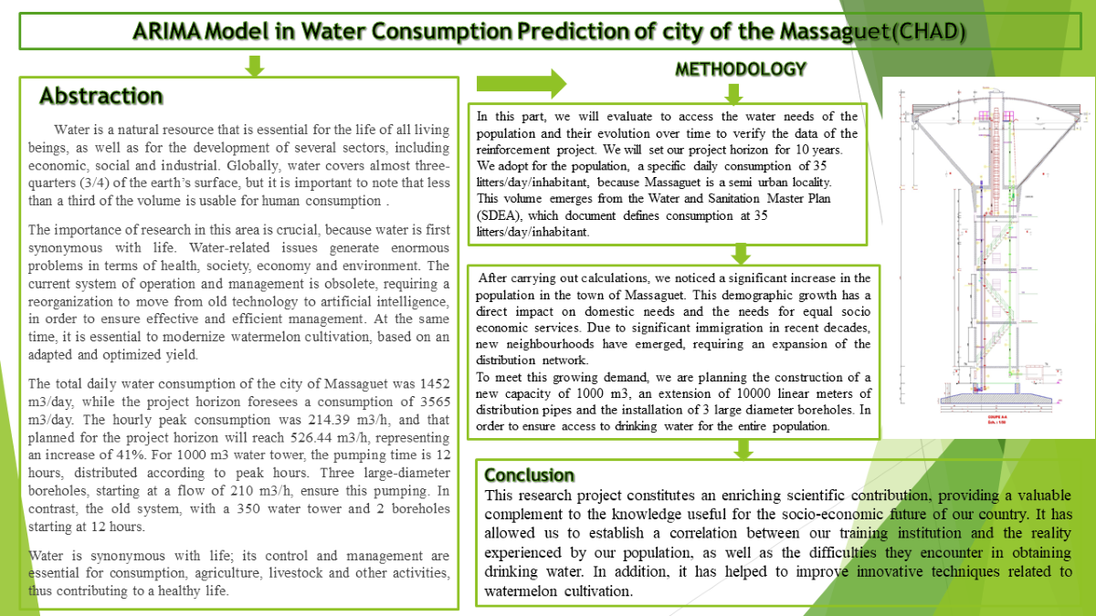
Water is a natural resource that is essential for the life of all living beings, as well as for the development of several sectors, including economic, social and industrial. Globally, water covers almost three-quarters (3/4) of the earth’s surface, but it is important to note that less than a third of the volume is usable for human consumption . The importance of research in this area is crucial, because water is first synonymous with life. Water-related issues generate enormous problems in terms of health, society, economy and environment. The current system of operation and management is obsolete, requiring a reorganization to move from old technology to artificial intelligence, in order to ensure effective and efficient management. At the same time, it is essential to modernize watermelon cultivation, based on an adapted and optimized yield. The total daily water consumption of the city of Massaguet was 1452 m3/day, while the project horizon foresees a consumption of 3565 m3/day. The hourly peak consumption was 214.39 m3/h, and that planned for the project horizon will reach 526.44 m3/h, representing an increase of 41%. For 1000 m3 water tower, the pumping time is 12 hours, distributed according to peak hours. Three large-diameter boreholes, starting at a flow of 210 m3/h, ensure this pumping. In contrast, the old system, with a 350 water tower and 2 boreholes starting at 12 hours. Water is synonymous with life; its control and management are essential for consumption, agriculture, livestock and other activities, thus contributing to a healthy life.

Keywords:

Drinking water

;

Arima

;

Water Consumption

Subject:

Engineering - Other

Introduction

Water is a natural resource essential to the life of all living beings, and even the development of several sectors (economic, social and industrial).

Indeed, globally, water covers nearly three- quarters (3/4) of the surface of the earth; it must also be said that less than 1/3 of volume is usable for human consumption [1].

For human beings, water is an essential resource. However, access to drinking water causes a major problem for the population. To meet this challenge, African States have committed through the Millennium Development Goal (MDG) to providing drinking water for more than 80% of the population and these are the reasons why the Chadian Government has considered strengthening the drinking water supply of the town of Massaguet [2].

In addition, on the sanitation plan, for a total Chadian population of 16,430,000 inhabitants (2020) according to the 2015 population demographic census, 1 out of 9 children dies before the age of five (years) that is 11.4% of infant mortality every year. A number of 16,590 people die each year due to lack of access of drinking water and sanitation source from The Ministry of Public Health [3].

Massaguet is currently estimated at 76,555 inhabitants in 2020 with a growth rate of 3.6% according to the source of INSEED (National Institute of Statistics, Economic and Demographic Studies) according to the 2015 population demographic census It is a semi-urban centre located at 82 km northeast of N’Djamena. Currently, the population’s access to drinking water is only 40% [4].

Comparing this to the overall rate of access to drinking water is very low.

The agricultural and livestock conflicts are very frequent and diseases linked to drinking water are recurrent, and those are the reasons why we chose the city of Massaguet to make a request for Reinforce and Innovate of the Drinking Water Supply of that city.

Massaguet, its economy is mainly based on agriculture, livestock and trade. The region has a large weekly market, which brings together several surrounding towns and villages every Sunday. The main crops grown during the season are corn, millet, sorghum, berebere and peanuts.

Additionally, they also grow produce such as watermelon, cucumber, onion etc., in the off-season [5].

Africa and presentation of Chad

As the world’s population continues to grow, the world’s problems with access to drinking water have become more and more serious, as a number of people in developing countries have no access to water; drinking water to meet most of their basic needs. Water resources exist and only about 1% would be enough the entire humanity.

However, this water is not even available to many people who have spent some huge amount of money or traveled far away to get the water they needed. In this regard, the government, the United Nations, the World Bank, the non-governmental organizations (NGO’s) and the local organizations sponsor all access projects of drinking water.

The geography of Chad consists of the study of the territory of Chad, a country with an area of 1,284,000 km², extending over 1,700 km from north to south and 1,000 km from east to west. Chad is the 5th largest country in Africa (after Algeria, the Democratic Republic of Congo, Sudan and Libya) and the 21st largest country in the world. The capital of Chad is N’Djamena.

Chad is located between the 7th and 24th degrees north latitude on the one hand and the 13th and 24th degrees east longitude on the other hand.

Chad has 5,968 km of land borders, distributed as follows: 1,360 km with Sudan; 1,197 km with the Central African Republic, 1,175 with Niger; 1,094 km with Cameroon 1, 055 km with Libya, and 87 km with Nigeria.

Figure 1. Localization of Chad.

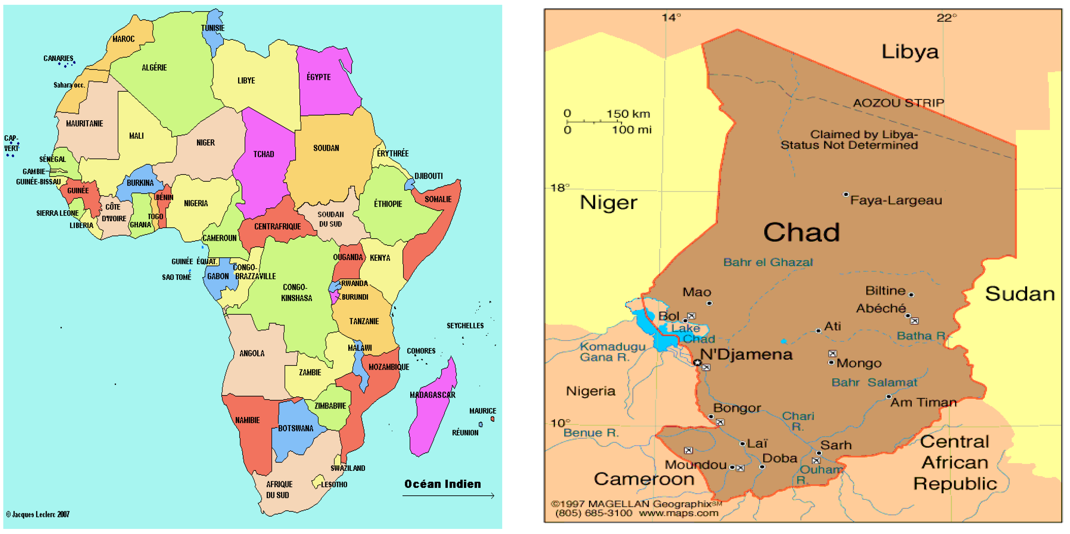
Chad has 1,284,000 square kilometers, the Capital is N’Djamena, and the foreign spoken languages are French, Arabic and English, and the local Arabic and Sara. The population of Chad was estimated at more than 16,000,000 inhabitants after 2020’s with growth rate of 3.6% according to the source of INSEED (National Institute of Statistics, Economic and Demographic Studies) [6,7].

Presentation of Massaguet City

Located in the Region of Hadjer Lamis, Massaguet is the capital of the department of Haraze Al Biar. The population of the city of Massaguet was estimated at 76,555 inhabitants in 2020’s with growth rate of 3.6% according to the source of INSEED (National Institute of Statistics, Economic and Demographic Studies). It is a semi-urban center located at 82 km northeast of N’Djamena [8].

Access to drinking water is only 40% of the population present. Most of the population gets its water from mini private castles and some motorized boreholes equipped with human pumps. The Chadian government recommends the strengthening of the drinking water supply system in the city of Massaguet to overcome food shortage, to grant access to drinking water all, and to intensify harmonious development.

The Figure 2 location of the project area. Massaguet is located in The Province of Hadjer Lamis, department of Haraze Albiar. The geographic coordinates of Massaguet are: Latitude 12.4667 (12°28’0’’) North, Longitude 15.4333, (15° 25’60’’) East and Altitude of Massaguet is 274 m [9].

Climate

Chad is a Sahelian country, located in the heart of Africa. Chad is made up of three climatic zones (Saharan, Sahelian and Sudanian).

The climate in Massaguet is of the Sahelian climate. The sparse vegetation is dominated by stunted shrubby species (neems, acacia etc.) [10].

Geology

It aims at understanding the nature, distribution, the history and the genesis of the constituents of the earth. Its objects of study belong to different levels of organization: crystal and metal, rock, rocky complex, structural complex (sedimentary basin), in relation to the different parts of the earth.

The area projected as part of the national territory is fortunately located in the hydro geologically favorable area that is to say in the Continental Terminal. Indeed, it is an area of ancient sedimentation with successive layers of clay and coarse sand and highlighting the presence of an abundant and continuous aquifer.

The large basins whose origin and development have been presented in the lithographically section. We recall the main ones:

(1)The Erdis or Precambrian basement is given about 3500 meters below the ground around 21°E, 20°N with 1500 meters of Nubian sandstone resting on 2000 meters of primary formation.

(2)The Doba basin where depth of the base would reach 7000 meters, with approximately 1000 meters of CT resting on some 6000 meters of Cretaceous;

(3)The Lake Chad which would reach 5000 meters deep; the basin fill corresponds to approximately 2000 meters of tertiary and Quaternary deposits and underlying Cretaceous sediments Evolution of Lake Chad from 1973 – 2013:

The Figure 3 shows us the impact of the climate change on the Lake on its surface areas, water volume and especially the agricultural and aquatic activities of the surrounding population [11].

The consequences of climate change (25,000 km² in 1960 and increased to 2,500 km² today).

(4) The others Cretaceous basins are those of Bousso and Salamat recognized a few sounding.

(5) Water resources: Especially in the Chari-Logone basin where are large flood plans. The basin has two types of groundwater: The water table flush between 20 – 30m, the deep free water table at more than 60m Massaguet is in a sedimentary zone with two aquifer levels [12].

Rainfall of Massaguet

The district of Massaguet, like the rest of the Chadian territory undergoes two seasons, including rainy season (existence of precipitation) and a dry season (absence of precipitation) source from Ministry of Civil Aviation [13].

Figure 4 sufficiently shows us a significant drop in rainfall for the years 2021 and 2022. This drop is undoubtedly due to climate change that has become not only a climatic scourge in Chad but internationally.

Temperature

Every day, in Massaguet, like the rest of the territory of the Republic of Chad, the sun in its apparent movement remains high in the sky. The obliquity of the solar rays being weak, the contribution of heat is maximum.

The intense heat between March and April characterizes the dry season. The maximum average of the temperature is around 40°C from March and April. The minimum average never drops below 20°C from December to February. This is a cold period in Massaguet [2,12].

Agriculture

Before the oil area (July 2003), farming was the important source of income in Chad, representing 24% of GDP and 80% of exports. The exports was based of four mains products, namely cotton, livestock, skins, Arabic gum. Even today, with the fall in oil prices, agro pastoral activities constitute, among others, (39 million ha of cultivable land (30% of the national territory), 5.6 million ha of irrigable land of which 335 000ha are easy to develop and more than 94 million heads of livestock, all species combine), a significant potential for a long-term growth of the economy and the effective means of reducing poverty in rural areas.

However, its potential is not fully exploited. Only 6% of the cultivable area is used. The causes are multiple: in addition to factors such as uncontrollable climatic variation, soil exhaustion, plant pests and inadequate water management, there is a particular difficulty that is a very limited access to inputs.

The increasing demand for water, fuelled by population growth, migration, rural displacement, and urbanisation, requires effective water management strategies in the Massaguet region in particular and Africa in general. Forecasting daily water supply, improve resource allocation, and plan for future needs. Many statistical and machine learning methods have been used to predict water consumption, each with its own advantages and challenges. Among these advantages and challenges, the ARIMA model has gained popularity due to its simplicity and robustness in handling time series data. This study aims to develop and evaluate an ARIMA model to forecast daily water consumption, and provide a comprehensive analysis of its applicability and performance in this context [14].

Materials and Methods

Data Collection

Data for our study was collected in accordance with the laid down procedures from different administrative departments. We followed legal administrative procedures by writing handwritten requests to the relevant departments. For instance, we contacted the Ministry of Water and Sanitation to obtain all the necessary hydrological data. We also turned to the Ministry of Civil Aviation and Meteorology, more precisely to the General Directorate of Meteorology, to obtain rainfall data.

In addition, we contacted the Ministry of Decentralization and Demography, in particular the General Directorate of the National Institute of Statistics, Economic and Demographic Studies, in order to obtain data from the population census in general, and more specifically data on the Massaguet.

Finally, we contacted the Ministry of Public Health, specifically the Directorate of Public Health, to obtain all the information relating to water related diseases and statistical data on death caused by water.

Field Visit

The field visit allowed us to carry out an assessment of the existing hydrological infrastructure. This visit was guided by those responsible for water management, reporting to the municipal commune of the city of Massaguet. The hydrological data that we collected reveal that the network is of the branched type, including a borehole with a flow rate of 54.38 m³/h which was carried out around 1958, as well approximately 150 m³/h which is currently out of commission and non-operational. The distribution network extends over a distance of 5000 linear meters. A few fire hydrants are present, 5 of which are functional and 6 of which are defective. In 2007, the city benefited from the installation of a new tower water with a capacity of 350 m³, two large diameter borehole with a depth of 72 meters, two generators with a power of 60 Kva/KW each, an extension of the distribution network over 10000 linear meters, as well as a few standpipes.

In addition, other water points in the locality, notably some mini solar reservoirs and human-powered pumps built by individuals.

Data Analysis

The data collected allows us to determine the demographics of the current population as well as those expected over the project horizon. In addition, they allow us to calculate all domestic water needs and socio-economic services. Finally, they help us to estimate the capacity needed for the construction of a new concrete castle to strengthen the drinking water supply system.

Applications of ARIMA Model in Water Consumption Prediction

The ARIMA model is a widely used statistical method for time series forecasting. Its application in water consumption forecasting stems from its ability to model temporal dependencies and trends in data. ARIMA models have been successfully used in a variety of contexts, including municipal water consumption agricultural irrigation demand, and industrial water consumption. These models are particularly effective in scenarios where historical data are available and the underlying trends are stable over time. By incorporating variances to handle nonstationary and combining autoregressive and moving average components, ARIMA models provide a flexible and powerful tool for forecasting water consumption [15].

Strengths and Limitations of ARIMA Model

The ARIMA model has several strengths that make it a valuable tool for time series forecasting, including water consumption forecasting. One of its main strengths is its ability to handle nonstationary data through variations, allowing it to effectively model seasonal trends and patters. In addition, the ARIMA model is relatively easy practitioners with varying levels of experience in time series analysis. The model’s flexibly in combining autoregressive and moving average components allows it to capture a wide range of temporal dependencies in the data. However, the ARIMA model also has limitations. It requires a large amount of historical data to produce accurate forecasts, and outliers and sudden changes in data patterns can affect its performance. In addition, ARIMA models assume linear relationships, which may not capture the complex, nonlinear interactions inherent in water consumption data. The models dependence on past values means that it may not perform well in the presence of structural breaks or external forcing factors that are not captured in the historical data [16].

Research Gaps and Opportunities

Despite the extensive use of ARIMA models in water consumption forecasting, there remain many research gaps and opportunities for further exploration. A major gap is the models limited ability to incorporate external variables, which can significantly affect water consumption patterns. Combining ARIMA models with other predictive techniques, such as machine learning algorithms or hybrid models, can improve their predictive accuracy and power. In addition, further research is needs on the performance of the models in different contexts and geographic regions, where water consumption patterns can vary considerably. Another area for further investigation is the development of methods to automatically identify and optimize model parameters, thereby reducing the need for manual tuning and specialized knowledge. Exploring the potential of ARMA models in real-time water consumption forecasting and integrating them into smart water management systems also presents interesting opportunities for improving water resource management practices [16].

Methodology

(1) Data collection and Preprocessing

The data collection phase involves collecting historical record of daily water consumption from relevant water management authorities of facilities. These data typically include the total volume of water consumed daily over a given period, as well as any additional information such as temperature, abstraction, and demographic statistics that may affect water consumption. Once available, the data undergo extensive Preprocessing to ensure their quality and suitability for analysis. This includes handling missing values, which can be handled by interpolation or imputation techniques. Outliers that may bias the model are identified and appropriately handled, by either transformation or deletion. Data stability is then checked, which is a prerequisite for ARIMA modelling. If instability is detected, various methods are applied to stabilize the average time series. In addition, the data are divided into training and test sets, the former being used to build the model and the latter to evaluate its performance [16].

ARIMA Model

The ARIMA model predict output variables via linear dependence on the stochastic term of its previous values. This model assumes time series data as stationary, and it is expressed as Equation, where p is the lag time of the ARIMA model, ∅ is the ARIMA coefficient, yt-1 is the previous values before t – 1 hours and εt is the error term.

yt = ∅1yt−1 + ∅2yt−2 + · · · + ∅pyt−p + εt = p ∑ i=1 ∅iyt−i + εt

The moving average (MA) model predict output variables using the error term (εt) of its previous values. This model assumes time series data as stationary, similar to the AR model, and it is expressed as Equation. Here q is the time of the MA model; µ is the mean of the series, andθis the MA coefficient.

yt = µ + εt + θ1εt−1 + θ2εt−2 + · · · + θqεt−q = µ + q ∑ i=1 θi εt−i + εt

The autoregressive moving average (ARIMA) model, which combines the ARIMA and MA models to predict a more accurate output variable, is expressed as Equation. The model is usually referred to as the ARMA (p, q) model, where p is the lag time of the part and q is the lag time of the MA part.

yt = ∅1yt−1 + ∅2yt−2 + · · · + ∅pyt−p + εt + θ1εt−1 + θ2εt−2 + · · · + θqεt−q

Box et al. proposed an ARIMA model that can be used with nonstationary time series data. The nonstationary time series is concerted into a stationary time series using the differencing. Here, the differencing in continuous observations, where B is the backward shift operator, ∆ is the differences, and d is the parameter of the differences [15,16].

∅p(B)∆ d yt= δ + θq(B) εt

ARIMA Model Development

ARIMA model development beings with identifying the appropriate order of the autoregressive (AR), differencing (I), and moving average (MA) components, denoted by (p,d,q). This process typically involves analysing autocorrelation (ACF) and partial autocorrelation (PACF) plots to determine the values of p and q, while the differencing process determines d. After specifying the model parameters, the ARIMA model is fitted to the training data using maximum likelihood estimation or another appropriate fitting method. Model performance is then evaluated using diagnostic checks, including residual analysis to ensure that the residuals are white noise, indicating a good fit. Various information criteria, such as the Akaike information criterion (AIC) or the Bayesian information criterion (BIC), are used to compare different models and select the best one. Once the optimal model is selected, it is used to predict daily water consumption on the test set. The accuracy of these predictions is evaluated using metrics such as mean absolute error (MAE), root mean square error (RMSE), and mean absolute percentage error (MAPE), providing a quantitative assessment of the model’s performance.

Model Evaluation and Selection

Model evaluation is a crucial step to ensure the reliability and accuracy of the ARMA model developed to predict daily water consumption. This process begins with a detailed diagnostic analysis of the model residuals to check for patterns or associations that the model fails to capture. The residuals should ideally behave like white noise, indicating that the model has correctly accounted for the structure of the data [16]. In addition to residual analysis, model performance is evaluated using different statistical measures. Mean absolute error (MAE), root mean square error (RMSE), and mean relative absolute error (MAPE), are commonly used to measure prediction errors and assess model accuracy. These metrics provide insight into the model performance both in sample (or training data) and out of sample (on testing data). Additionally, information criteria such as the Akaike information criteria (AIC) and the Bayesian information criteria (BIC) are used to compare different ARIMA models, balancing model fit and complexity. The model with the lowest Akaike information criteria or Bayesian information criteria is generally preferred, as it indicates a better balance between model fit and economics. Based on these evaluations, the best performing ARIMA model is selected for forecasting [16,17].

Prediction and Analysis

Once the optimal ARIMA model is selected, it is used to generate forecast of daily water consumption. The forecasting phase involves applying the model to a test data set and generating forecasts of future water consumption. These forecasts are then compared to actual observed values to assess their accuracy and reliability [17]. The analysis goes beyond simply assessing the accuracy of the forecasts; it also involves examining the forecasted values to identify emerging trends or patterns in water consumption. Factors such as seasonal changes, holidays, and special events that may affect water consumption are analysed to understand their impact on the forecasts. In addition, a scenario analysis can be performed to explore the effects of potential changes in influencing factors, such as significant weather events or policy changes. The information obtained from this analysis is essential for making informed decisions in water resources management, such as adjusting supply levels, planning infrastructure investments and implementing water conservation measures. The predictive capabilities of the ARIMA model therefore provide a valuable tool for short-term operational decisions and long-term strategic planning in water resources management [17,18].

Introduction to Python

Python is a high-level, general-purpose programming language created by Guido van Rossum and first released in 1991. It is known for its simplicity and readability, making and ideal choice for both beginners and experienced programmers. Python’s core philosophy centres on code readability and the use of large spaces, making complex applications easy to write and maintain.

Python support multiple programming styles, including procedural, object-oriented, and functional programming, making it suitable for a wide range of tasks, from simple scripts to complex machine learning models. Over the years, Python has become one of the most popular languages, particularly in fields such as data analysis scientific computing, artificial intelligence, and web development.

(1) Python’s Significance in Data Analysis and Machine Learning

Python plays a vital role in the fields of data analytics machine learning due to its simplicity, flexibility, and vast ecosystem of libraries that support a wide range of tasks. The importance of Python in these fields can be highlighted in several key areas: Easy to learn and use: Python’s simple structure emphasizes readability, which reduces the cost of maintaining the program.

Interpreted language: Python is processed at runtime by the complier. This means that you do not need to compile your code before running it, which speeds up development. Dynamic typing: Python allows us to declare variables without explicitly declaring their type, thus providing greater flexibility. Comprehensive libraries: Python contains a rich ecosystem of libraries that enable a wide range of applications. Some of the most popular ones include Pandas, NumPy, Matplotlid, and TensorFlow.Cross-platform: Python is platform-independent, which means that we can run the same code on different operating systems like Windows, Mac, and Linux without modification [19,20].

Method and Material

For this project, we analyzed water consumption data multiple sources, focusing on daily requirements and peak demands for different sectors. The dataset contains variable such as total daily water requirement (Tdw), peak day needs (Pdn) and hourly peak needs (Qp) among others (ARIMA Model prediction).

We used the Pandas library to load and preprocess the data. The dataset was organized as table and required cleaning and handling of missing values. The following Python code snippet shows how to load data:

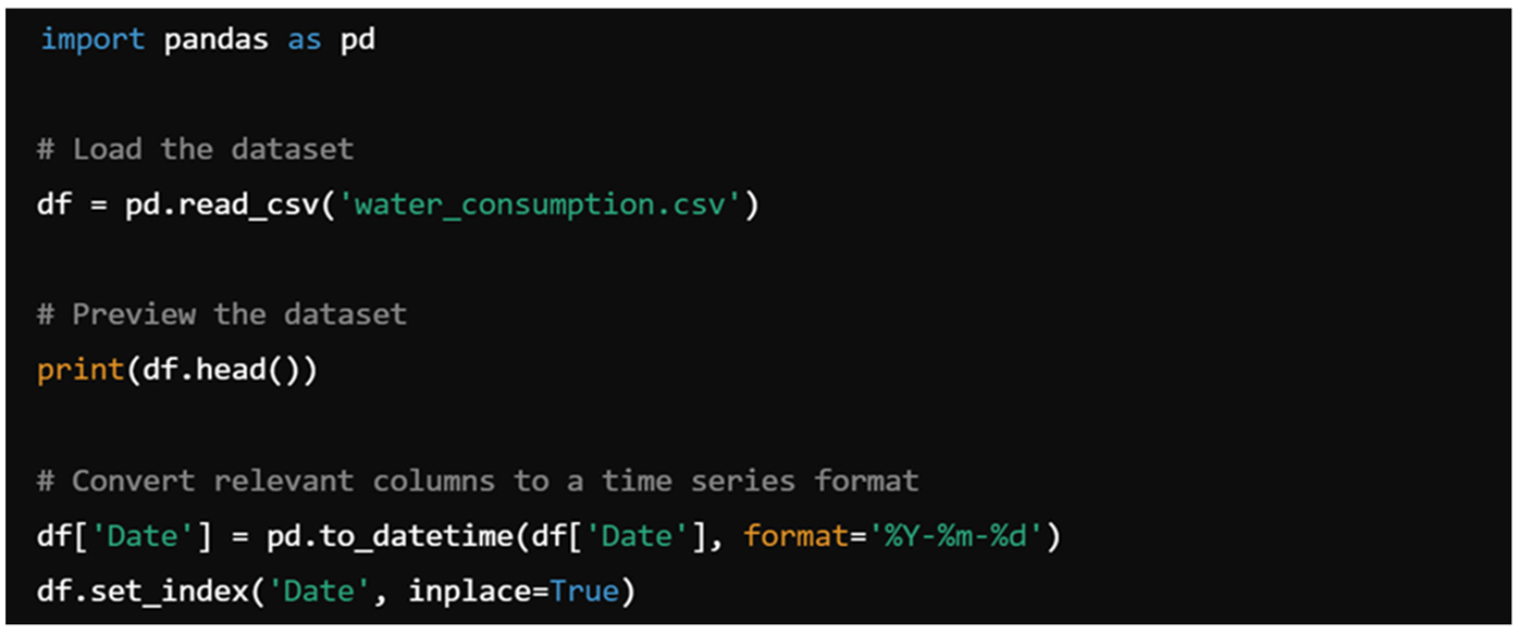
The preprocessing steps included converting the data column into a date time format to allow for time series manipulation. Once the data was cleaned, we could move on to model fitting.

Exploratory Data Analysis (EDA), before fitting the ARIMA model, we conducted exploratory data analysis using Matplotlid and Seaborn to visualize data trends, utilizers, and water consumption patterns. Below is a graphical example of total daily water requirements (Tdw) over time:

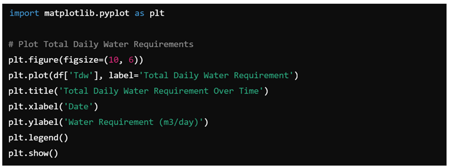
This visualization helped us understand the water consumption behavior, which was crucial in choosing the right parameters for the ARIMA model.

The ARIMA (Autoregressive Integrated Moving Average) model is widely used to display time series. Here, the implement the ARIMA model to prepare the future water consumption based on the historical basis.

The process of fitting the ARIMA model is to select the parameters: (p, d, q). this will satisfy the auto part (P), the difference level (d), and the mobile part (q). We have used an automatic model selection process to identify the optimal parameters, as shown in the following code:

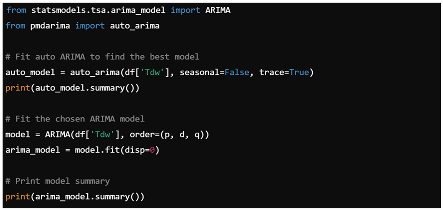
The auto_arima function of the PMarima package automates the process of function of finding the best parameters, facilitating optimal model fitting. The fitted model was then used to predict future water consumption.

After fitting the model, we predicted future water consumption values and visualized the forecasts using the original data. Below is the code to create and graph the forecasts:

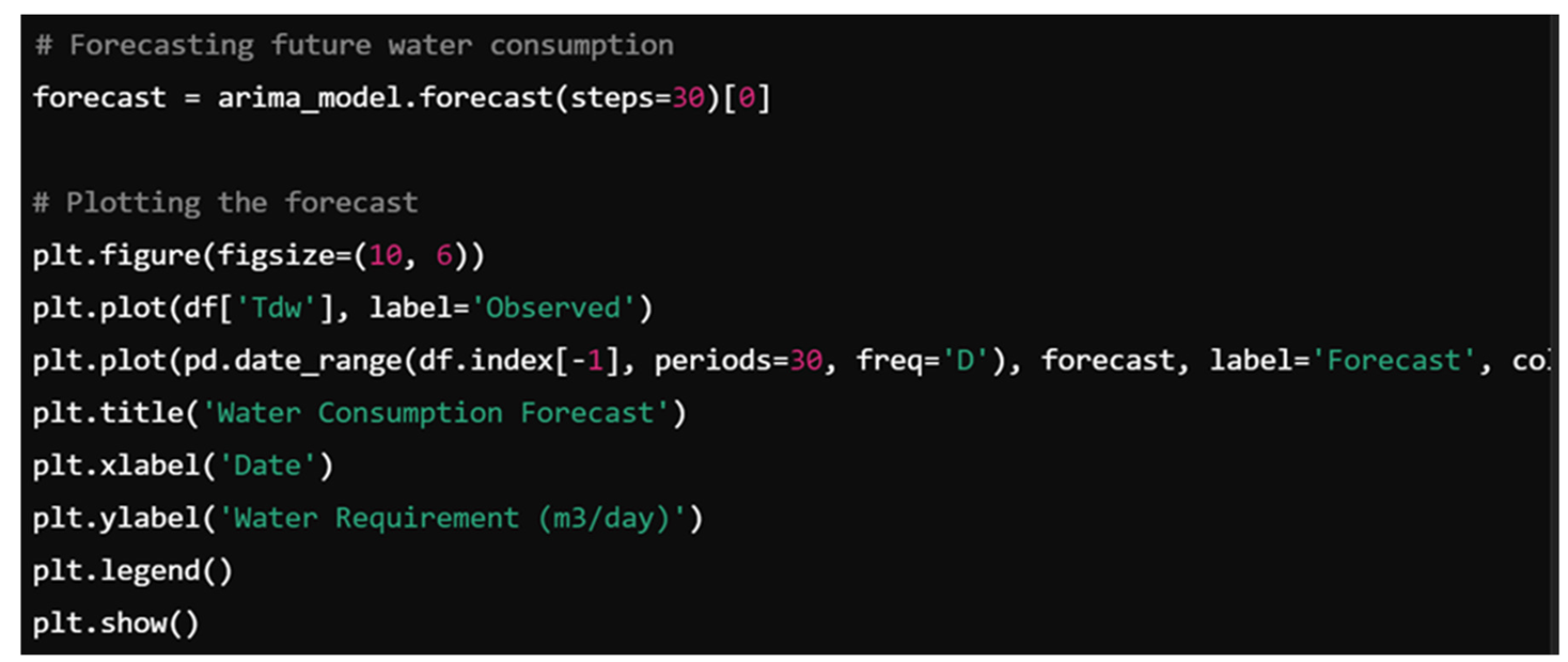
The figure obtained at this stage shows the expected water consumption over the next 30 days, which helps guide water management strategies. As shown in the dataset (Arima_model_prediction), peak daily demand (Pdn) and peak hourly consumption (Hpd) show significant variations, highlighting the importance of accurate forecast to plan for extreme scenarios.

Results and Discussion

Figure 5 showcases the ARIMA model is forecast of various water consumption metrics from 2020 to 2033. This figure is integrate for understanding now different aspects of water demand are expected to evolve over time, valuable insights for water resource management and planning.

(1) Time-Series Forecasting and the Role of ARIMA

The ARIMA model, known for its strength in time-series forecasting, has been employed to project future water consumption based on historical data. The forecast period spans from 2020 to 2033, and the model generates predictions for multiple water usage metrics. These metrics are likely on the Y-axis (representing the volume of water in cubic meters) against time on the X-axis (years).

(2) Trends in population Water Needs (Adwc)

One of the primary metrics forecast is the daily water needs of the population, labelled as Adwc. In 2020, the water need for the population is recorded at 1,210 m³/day. This figure is projected to increase significantly, reaching 2971 m³/day by 2033. This substantial growth reflects the impact of population increase and possibly changes in per capita water consumption. It underscores the need for expanding water infrastructure to meet the rising demand.

(3) Socio-Economic Services Water Needs (Wss)

The water needs for socio-economic services, indicated as “Wss” start at 242 m³/day in 2020 and are forecast to surge to 2971 m³/day by 2033. The sharp rise in this metric indicates that economic growth, urbanization, and the expansion of industrial and service sectors are driving up water demand. The convergence of this metric with population water needs by 2033 suggest that socio-economic activities will play an increasingly significant role in overall consumption.

(4) Total Daily Water Requirement (Tdw)

The total daily requirement labelled “Tdw” is a summation of various water demands, and it starts at 1452 m³/day in 2020, reaching 3565 m³/day by 2033. This metric provides a holistic view of the daily water consumption needs and highlights the cumulative impact of rising population and economic activities. The steady upward trend signifies a growing pressure on water resources, which necessitates proactive management and efficient distribution strategies.

(5) Average Daily Requirement of the Peak Month (Npm)

The “Npm” represents the average daily requirement during the peak consumption month. It begins at 1597.20 m³/day in 2020 and is forecast to grow to 3922 m³/day by 2033. The initial high value in 2020 suggest that there might have been an exceptionally high water demand during a specific month, which could be due to seasonal variations, such as dry months, or specific event causing a spike in usage. The gradual decline in this value by 2033 could indicate a stabilization or more evenly distributed water usage throughout the year.

(6) Peak Day Need (Pdn)

The peak daily need measured, denoted “Pdn’’, which assesses the maximum daily water requirements, was 1884.69 m³/day in 2020 and is projected to reach to 4628 m³/day by 2033. This increase in daily requirements is linked to population increase of 63% compared to the total population in 2020.

(7) Regarding Hourly Peak Demand (Qp) and Hourly Peak Consumption (Hpd):

“Qp”refers to the peak hourly water demand, which was 78.53 m³/hour in 2020 and is expected to increase significantly to 193 m³/hour by 2033, due to population growth. Similarly, “Hpd” or hourly peak consumption started at 214.39 m³/hour in 2020 and is theoretically projected to reach to 526.44 m³/hour 2033.

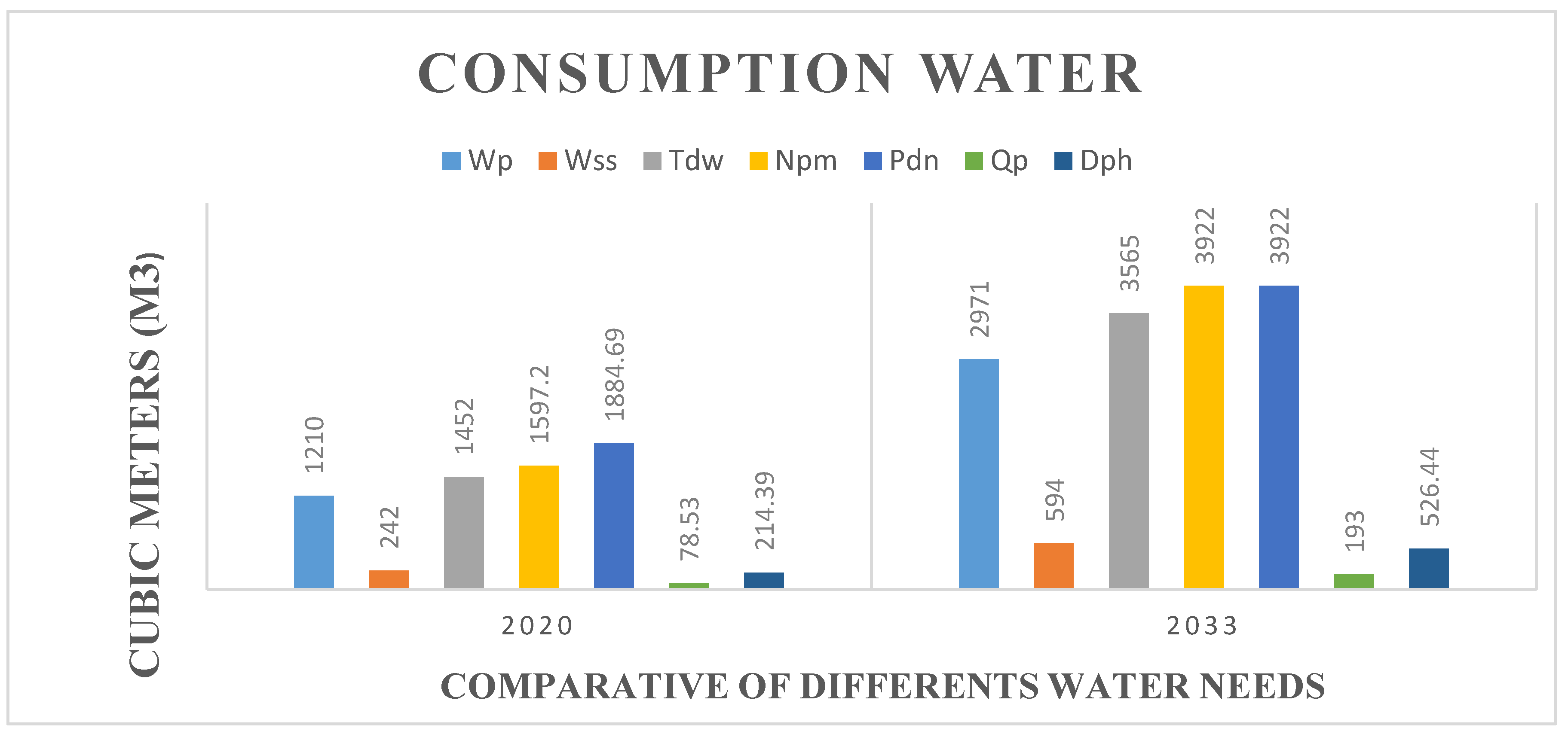
Table 5. Data for forecast for multiple water consumption metrics.

N°	consumption water	2020	2033
1	water needs of the population (Adwc)	1210 m³/day	2971 m³/day
2	water needs of socio-economic services (Wss)	242 m³/day	2971 m³/day
3	Total daily water requirement (Tdw)	1452 m³/day	3565 m³/day
4	Average daily requirement of the peak month (Npm)	1597.20 m³/day	3922 m³/day
5	Peak day need (Pdn)	1884.69 m³/day	4628 m³/day
6	Hourly peak demand (Qp)	78.53 m³/hour	193 m³/hour
7	Hourly peak consumption (Hpd)	214.39 m³/hour	526.44 m³/hour

These increases suggest a shift toward more consistent and controlled water use patterns, likely driven by technological advances, water management systems, and perhaps a more conscious effort to distribute water evenly throughout the day.

(8) Overall Interpretation and Implications

Figure 6. Comparative of different water needs.

Rising Trends in Overall Demand: The consistent upward trend in most metrics, Such as Adwc, Wss and Tdw, signals that overall water demand is expected to grow substantially. This growth reflects broader socio-economic trends, including population growth and economic development, which will increase pressure or existing water resources.

Management of Peak Demands: The reduction in peak day needs and hourly peak demands highlights efforts or expectations to manage and reduce extreme spikes in water usage. This could be through better demand management, infrastructure improvements, or shifts in consumer behaviour towards more sustainable water usage.

Need for Strategic planning: The data in Figure 5.1 underscores the critical need for strategic planning in water resource management. Authorities will need to ensure that infrastructure development keeps pace with the rising demand, while also implementing policies and technologies that can mitigate impact of peak demand periods.

Overview of Figure 7 ARIMA Model Forecast for Multiple Water Consumption Metrics, Figure 5.1 presents the forecast results of the ARIMA model applied to predict various water consumption metrics over a specified period. The figure likely visualizes the expected in water consumption metrics such as daily water requirement, peak day needs, hourly peak demand, and from, the year 2020 to 2033.

Key points from the figure:

(1) Time-series Forecast:

The ARIMA model is used for predicting future values based on historical data. In this water figure, we can see projections of different water consumption metrics over time, from 2020 to 2033.

(2) Rising Trends:

The forecast shows a consistent increase across different metrics, reflecting growing water demand over time. For instance, the water needs of the population (Adwc) are projected to rise from 1210 m³/day in 2020 to 2971 m³/day by 2033.

(3) Comparison between Metrics:

Each water consumption metrics is plotted separately, which allows for a comparative analysis. Metrics like the total daily water requirement (Tdw) and peak day need (Pdn) exhibit significant increase, which indicate heightened demand during peak periods.

(4) Peak Demands:

The figure likely highlights the projected values for peak month and peak day demand, showing the highest water consumption expected. For instance, the peak day need (Pdn) is forecasted to increase form 1884.69 m³/day in 2020 to 4628 m³/day by 2033.

(5) Hourly Variations:

Hourly peak demand (Qp) and hourly peak consumption (Hpd) are also shown, reflecting the fluctuations in water usage on an hourly basis. These metrics are crucial for understanding short-term spikes in water demand, which could be driven by factors like population growth or increased socio-economic activities.

(6) Interpretation:

The figure illustrates that as the population grows and socio-economic activities expand, there will be a significant rise in water demand across various metrics. The ARIMA model helps in capturing these trends, providing a forecast that can be used for planning and managing water resources effectively. The consistent upward trend across all metrics suggest that there is a pressing need for enhanced water management strategies to meet the future demands predicted by the ARIMA model.

Proactive Measure Required: The ARIMA model’s projections provide a clear indication that water demand will continue to grow, necessitating proactive measure in terms of infrastructure, policy and technology to ensure sustainable water supply. The model’s ability to highlight both long-term trends and potential shifts in peak demand patterns offers valuable insights for decision –makers in the water management sector.

This detailed interpretation provides a comprehensive understanding of the forecast water consumption trends and their implications, which are crucial effective water resource management and planning.

Conclusion

This research project constitutes an enriching scientific contribution, providing a valuable complement to the knowledge useful for the socio-economic future of our country. It has allowed us to establish a correlation between our training institution and the reality experienced by our population, as well as the difficulties they encounter in obtaining drinking water. In addition, it has helped to improve innovative techniques related to watermelon cultivation.

We encourage our colleagues to choose similar projects in the future, in order to help donors and government provide substantial resources to address the challenges in our cities, towns and sub-regions.

The resulting resolution involves the reinforcement of a 1000 cubic meter water tower and the installation of linear distribution pipes. The innovation lies in the installation of a water supply system using artificial intelligence, as well as automatically programmed pumping. This system also includes an automatic distribution using various parameters and accessories (software, bank account, etc.) to ensure good water sustainability, as well as the implementation of a drip irrigation system for watermelon cultivation, while ensuring transparent and rational management of water revenues.

The expected results are considerable. These solutions will be essential to solve problems related to waterborne diseases, infant mortality, conflicts between farmers and herders, the development of watermelon crops, as well as the sustainability of drinking water for the population. The implementation and adaption of this new system in other cities will undoubtedly contribute to the Chadian government’s development plan, aiming for 80% access to drinking water by 2030, as well as the autonomy and development of the agricultural system throughout the territory.

References

Oki T, Entekhabi D, Harrold T I J G E, et al. The global water cycle[J], 1999, 10:27.
Verdeil V, Verspyck R, Adamou Maiga T, et al. Chad-Water and Sanitation Sector Note[J], 2019.
Mbaigoto N, Alsharif K, Landry S J S W R M. An assessment of the degree of the implementation of the integrated water resources management principles in the Lake Chad Basin: the case of the Republic of Chad[J], 2023, 9(4):118.
Azevedo M J, Decalo S. Historical dictionary of Chad[M]. Rowman & Littlefield, 2018.
Kadjangaba E, Bongo D, Le Bandoumel M J O J O M H. Adequacy of Water Use Resources for Drinking and Irrigation, Study Case of Sarh City, Capital of Moyen-Chari Province, CHAD[J], 2022, 13(1):1-21.
Kneib, M. Chad[M]. Marshall Cavendish, 2007.
Organ, J. Chad: Human Fertility, Crop Production and Changing Weather Patterns[D]. The University of New Mexico, 2020.
Dibe G P, Diarra M C J E I W A. Chad: An overview, trends and futures[J], 2015, 29:119.
Nour A M, Abderamane H, Ngatcha B N, et al. Characterization and Aquifer Functioning System of Haraz Al Biar (North Chari Baguirmi)[J], 2017, 5(12):52-64.
Pham-Duc B, Sylvestre F, Papa F, et al. The Lake Chad hydrology under current climate change[J], 2020, 10(1):1-10.
Ruppel O C, Funteh M B. Climate change, human security and the humanitarian crisis in the Lake Chad Basin region: selected legal and developmental aspects with a special focus on water governance[C]. Law| Environment| Africa, 2019:105-136.
Olowoyeye O S, Kanwar R S J S. Water and food sustainability in the Riparian countries of Lake Chad in Africa[J], 2023, 15(13):10009.
Denton, M. Chad[M]. Cavendish Square Publishing, LLC, 2021.
Pereira D R M, Nascimento A D R, Lima M F, et al. Agronomic performance of watermelon under direct sowing system and seedling transplanting[J], 2022, 40(1):23-32.
Nie S, Liu Q, Ji H, et al. Integration of ARIMA and LSTM models for remaining useful life prediction of a water hydraulic high-speed on/off valve[J], 2022, 12(16):8071.
Du H, Zhao Z, Xue H J W. ARIMA-M: A new model for daily water consumption prediction based on the autoregressive integrated moving average model and the Markov chain error correction[J], 2020, 12(3):760.
Sharma A K, Punj P, Kumar N, et al. Lifetime prediction of a hydraulic pump using ARIMA model[J], 2024, 49(2):1713-1725.
Mahmood R, Jia S, Mahmood T, et al. Predicted and projected water resources changes in the chari catchment, the lake chad basin, africa[J], 2020, 21(1):73-91.
Lutz, M. Programming python[M]. “ O’Reilly Media, Inc.”, 2010.
Van Rossum, G. Python programming language[C]. USENIX annual technical conference, 2007:1-36.

Figure 2. Localization of project zone.

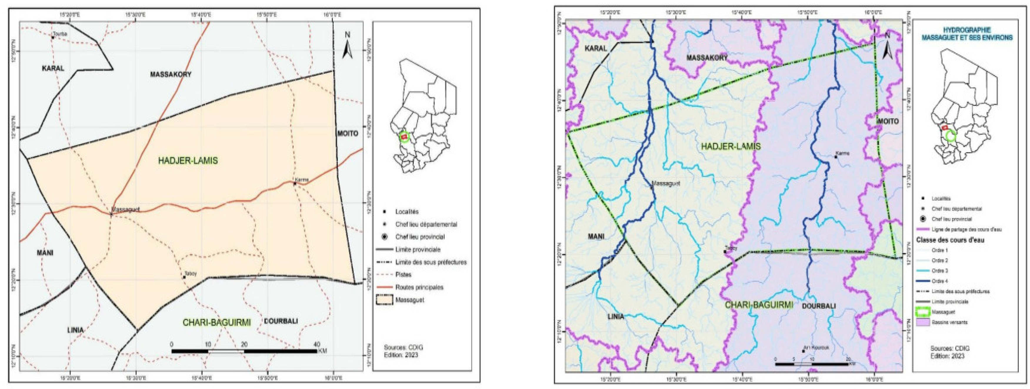
Figure 3. situation of Lake Chad.

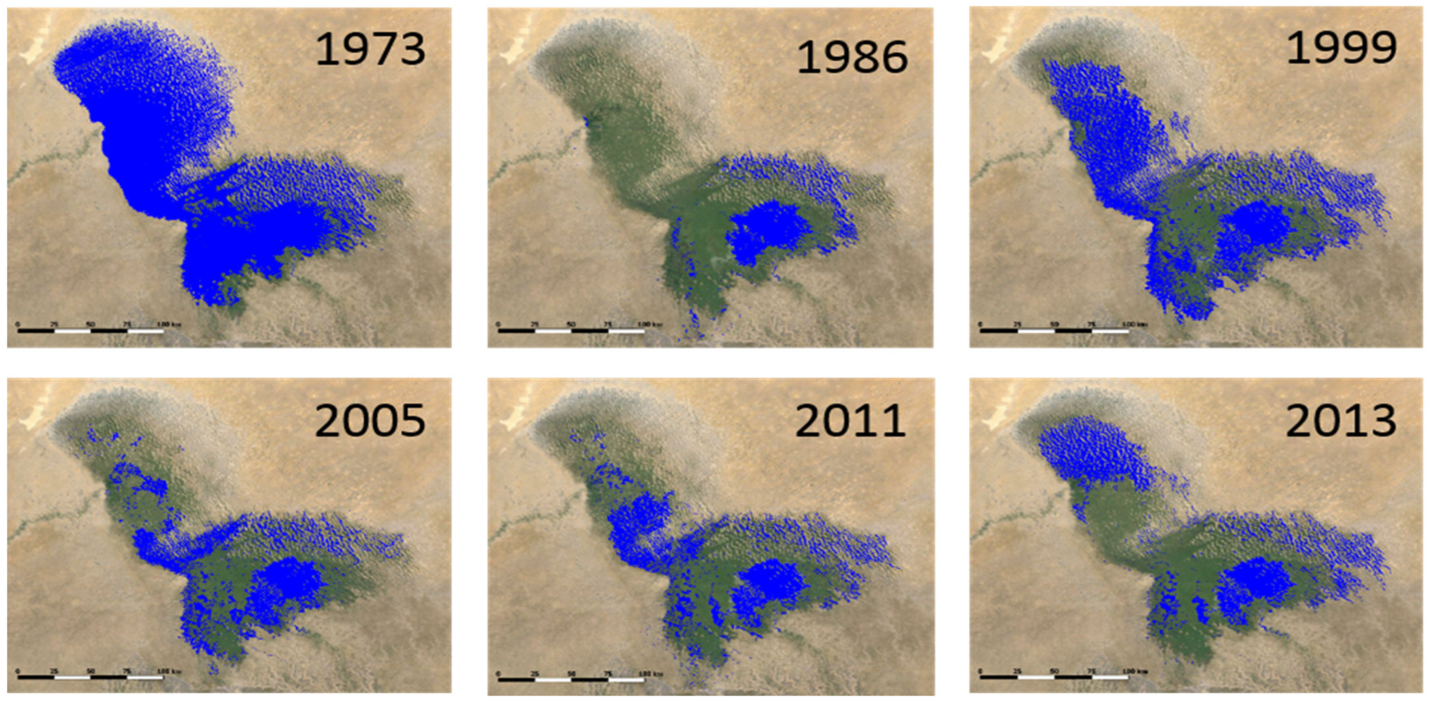
Figure 4. Rainfall of Massaguet.

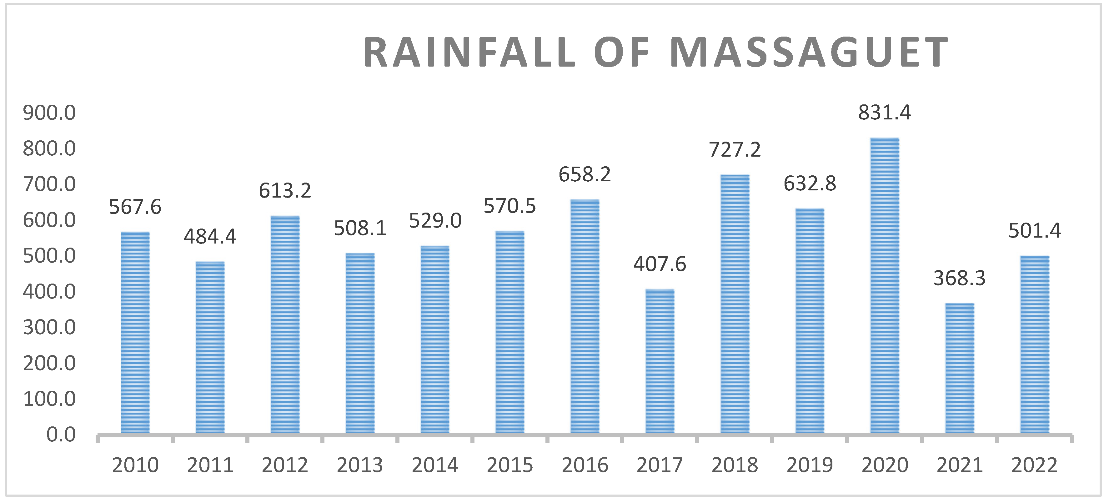
Figure 7. Arima model forecast for multiple water consumption metric.

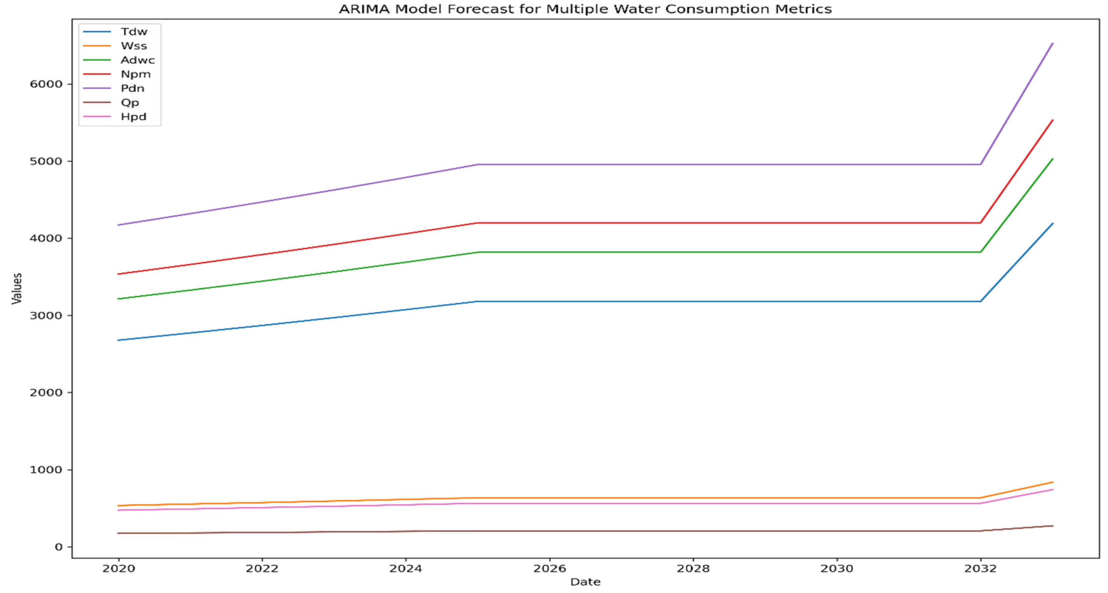
Table 1. Rainfall (in mm) at the Ndjamena Airport station.

Year	Jan	Feb	Mar	April	Mai	Jun	Jul	Aug	Sep	Oct	Nov	Dec	Total
2010	0,0	0,0	0,0	0,0	1,8	51,5	215,2	122,6	155,7	20,7	0,0	0,0	567,6
2011	0,0	0,0	0,0	0,0	10,8	77,2	59,6	180,6	156,2	0,0	0,0	0,0	484,4
2012	0,0	0,0	0,0	0,0	30,1	53,8	154,3	266,9	94,3	13,8	0,0	0,0	613,2
2013	0,0	0,0	0,0	0,0	3,3	26,6	140,5	249,9	86,1	1,7	0,0	0,0	508,1
2014	0,0	0,0	0,0	1,9	28,4	4,6	173,1	189,8	114,1	17,1	0,0	0,0	529,0
2015	0,0	0,0	0,0	0,0	0,9	81,2	243,4	162,0	81,9	1,1	0,0	0,0	570,5
2016	0,0	0,0	0,0	0,0	25,8	47,9	211,2	210,4	137,7	25,2	0,0	0,0	658,2
2017	0,0	0,0	0,0	0,0	27,8	49,1	153,9	134,4	42,4	0,0	0,0	0,0	407,6
2018	0,0	0,0	0,0	0,0	49,8	58,7	300,7	227,5	74,3	16,2	0,0	0,0	727,2
2019	0,0	0,0	0,0	0,0	65,2	58,1	180,4	141,3	128,7	59,1	0,0	0,0	632,8
2020	0,0	0,0	0,0	0,0	4,4	35,6	271,9	334,5	185,0	0,0	0,0	0,0	831,4
2021	0,0	0,0	0,0	0,3	0,7	60,6	107,3	102,0	78,8	18,6	0,0	0,0	368,3
2022	0,0	0,0	0,0	17,8	18,2	22,6	184,8	194,8	63,2	0,0	0,0	0,0	501,4

Disclaimer/Publisher’s Note: The statements, opinions and data contained in all publications are solely those of the individual author(s) and contributor(s) and not of MDPI and/or the editor(s). MDPI and/or the editor(s) disclaim responsibility for any injury to people or property resulting from any ideas, methods, instructions or products referred to in the content.

© 2024 by the authors. Licensee MDPI, Basel, Switzerland. This article is an open access article distributed under the terms and conditions of the Creative Commons Attribution (CC BY) license (http://creativecommons.org/licenses/by/4.0/).

Copyright: This open access article is published under a Creative Commons CC BY 4.0 license, which permit the free download, distribution, and reuse, provided that the author and preprint are cited in any reuse.