New Insights from Sadi Carnot’s Reflections of 1824: Gibbs Field Energy from Greenhouse Gases Recycled by the Virial Theorem with Gravity, Optimising Elevation of the Tropo-sphere and Surface Temperatures

Two centuries after Carnot defined thermodynamics as a scientific discipline based on work by engineers like James Watt, can we learn more from Carnot’s perceptive analysis of maximum power from heat engines? Using action mechanics, the rate of work in Carnot’s heat engine cycle can be integrated as external pressure-volume work, sustained by internal quantum field work, equal to changes in Gibbs free energy that was called caloric by Carnot. His treatise of 1824 even gave equations that express the work potential as a function of temperature and the logarithm of the change in volume. To answer this question, we apply Carnot’s principle defined by Clausius as entropy, to atmospheric heat-work cycles, such as in anticyclones. We show using Lagrange’s virial theorem how Carnot’s thermodynamic states as Gibbs potential become entangled with gravitational potential states. The effective capacitance of greenhouse gases for energy in the troposphere enable recycling of heat emitted from the Earth’s hot surface, thermally setting tropospheric air masses in action. By delaying irreversible emission of long wavelength quanta to space, this recycling process extends the residence time of solar energy in the troposphere as work, maximising troposphere entropy to the tropopause. The virial theorems of Lagrange and Clausius, governed on the principle of least action, provide a more accurate lapse rate in temperature with temperature in the atmosphere, replacing the paradigm of adiabatic expansion. Reversible 4-stage Carnot cycles, based on Lagrangian least variation in action, raise surface temperature and pressure from turbulent heat release, sustaining the weight of the atmosphere. New lessons for understanding climate dynamics are emerging from this virial-action analysis.

Keywords:

Carnot cycles

;

Gibbs energy

;

Lagrangian analysis

;

virial lapse rate

;

adiabatic lapse rate

;

principle least action

;

greenhouse gases

;

gravitational energy

;

tropopause

;

Gibbs quantum field

Subject:

Environmental and Earth Sciences - Space and Planetary Science

Supplementary Material

supplementary.pdf (9.12MB )

1. Introduction

In previous articles [1,2], we showed how the Carnot cycle can be explained by action mechanics, regarding caloric as Gibbs field quanta [1]. Thermodynamic properties such as entropy and the Gibbs energy of the gas molecules are easily calculated from molecular properties, temperature and pressure allowing the entropy and free energy of atmospheric gases to be calculate correct to four significant figures [1]. This is consistent with statistical mechanics, interpreting Gibbs phase space of momentum and position as least action space. Carnot [3] anticipated Gibbs free energy as two kinds of caloric at hot and cold temperatures and the ‘chute’ between them. His expressions that “the quantity of heat due to the change in volume of a gas is greater as the temperature is higher” and “The fall of caloric produces more motive power at inferior than at superior temperatures” are consistent with current theory. These principles indicate that the variation in Gibbs energy is a function of both volume and temperature with maximum work possible when the temperature difference between the hot source and the cooling sink is greatest, the latter as low as possible. In action mechanics, the maximum work possible is estimated as the variation in Gibbs energies of the heating isothermal gas and of the cooled isothermal gas [2]. Carnot also remarked that coal could potentially achieve a temperature difference of 1000 ^oC, whereas the steam engines then current were designed to work over a range of temperatures of only 60 ^oC [3].

Isothermally, the enthalpy and total energy of a gas remains constant, Carnot showed that the property that Clausius later defined [4] as entropy was a function not only of the temperature but also the diminishing density of the molecule, expressed as the logarithm of its volume. Carnot was clearly already aware of the conservation of total kinetic and potential energy in natural systems. This observation was known since Leibniz explained that the vis viva was stored reversibly in potential, described brilliantly later as energy by Emilie du Chatelet [5]. So both the first and the second energy principles emerged from Carnot’s work published in 1824 [3]. Entropy defined as the Carnot principle is a function of state that measures the extent to which the energy is stored as internal work or dissipated more generally. In quantum terms, the negative Gibbs energy tends to become greater, achieving a state with a greater quantum number measured as scalar action, able to be estimated as a logarithmic function of the quantum number [6,7].

A heat engine cycle (Figure 1) involves charging a working fluid with heat isothermally at a high temperature, increasing its quantum state number by expansion while doing external work; then allowing it to continue expanding adiabatically with no change in quantum state as temperature decreases, compensated by the increased dilution of each molecule. Carnot’s stage three of compression by the engine’s inertia reduces quantum number per molecule isothermally by removing heat supporting action to the original quantum number. The cycle is concluded by continued adiabatic compression restoring the original temperature and pressure and quantum state. Carnot explained this process exactly [3] using the varying caloric content for the modern quantum state, referring to two heating stages of the working fluid (a + b) and two cooling stages (b’ + a’) in the cycle. Acting together, these four processes ensure that the cycle is reversibl, inferring that the magnitude of the maximum work possible is given by (a – a’) or (b’ – b).

A key conclusion in the reversible Carnot cycle as explained by Clausius and Kelvin is that the entropy change for heat transfer inwards in stage 1 (+q/T₁) is equal to the entropy change for heat transfer outwards in stage 3 (-q/T²), so that the variation in scalar action in stage 1 is equal to that in stage 3, whereas the change in Gibbs energy in each stage is proportional to the temperature [2].

Carnot was also aware that the maximum engine power predicted was not achievable. The mechanism of two isothermal heat transfers across a fall in temperature linked by adiabatic expansions and compressions is an ideal proposal not possible in practice. Real engine systems are neither isothermal nor adiabatic and includes frictional losses. In this article, we will show how Carnot’s treatise of 1824 on the motive power of heat can be related to meteorological processes in the real troposphere. Can more be done to relate Carnot’s principles to atmospheric and meteorological science? We claim it can, particularly when the principles of least action initiated by Leibniz and expressed in Lagrange’s calculus of variations are integrated, requiring action mechanics to simplify calculations. Just as for the Carnot cycle in real engines, there is dissipation of energy during all these cycles so that the Lagrangian relationship does not achieve equality between the two terms of the Euler-Lagrange equation. In fact, this dissipative frictional property is important for heating the Earth’s surface in anticyclones from heat stored as work [7], that we will show is facilitated by greenhouse gases.

2. Materials and Methods

To apply the Carnot cycle to the troposphere requires calculation of entropy and Gibbs free energy of an ideal gas using action mechanics [1,2], a new method is needed to incorporate gravitational potential into atmospheric dynamics. This requires the novel use of the Lagrangian virial theorem to estimate lapse rates in temperature with altitude [9]. Essentially, the virial theorem shows that the mean vis viva (

\sum_{1}^{n} m v^{2}

) in a set of interacting particles subject to central forces is equal to their average potential energy. Thus, the mean kinetic energy (T=Σmv²/2) in such a Lagrangian system is half the mean potential energy.

\sum_{1}^{n} m v^{2}) / 2 n = T

(1)

2.1. Action Mechanics

Action mechanics reinterprets the partition functions given in textbooks on statistical mechanics as estimates of scalar action, with units measured with Planck’s quantum of action (h). For diatomic gases like N₂ and O₂, comprising 99% of the atmosphere, the macroscopic variables of temperature and volume or density expressing entropy (S) and entropic heat (ST) of statistical mechanics [10] have been integrated in simplified form [1,2,6] as functions of scalar action. Translational action (@_t=mrvδφ) and rotational action is designated as having dimensions similar to the vector angular momentum and rotational action (@_r=Iω/σ) including factors for symmetry (σ) and the ratio of mean velocity to root mean square velocity (z_t). Then the terms in equations (2) and (3) from statistical mechanics for translation and rotation [10] can be expressed in equations (4) and (5) as terms of action in quantum fields by quantum numbers, yielding field energies able to be expressed as mean values for individual molecular quantum fields [6].

S_tT= RTln[e^5/2 (3kTI_t)^3/2/(ħ³z_tσ)] Translational entropic energy

(2)

S_rT = RTln[{8π²(8π³I_AI_BI_C)^1/2(kT)^3/2}/σ_rh³] + 3/2RT 3-dimensional rotation

(3)

ST = RTln[e^9/2(@_t/ħ)³(@_r/ħ)²] Translation + 2-dimensional rotation as action (@)

(4)

= RTln[e^9/2n_t³j_r²] Given as action quantum numbers, n_t and j_r

(5)

For these equations for linear diatomic gases (Figure 2), the equivalence of macroscopic properties of temperature and pressure are shown as logarithmic ratios of action (@/ħ), using Planck’s reduced constant (ħ) in the denominator to measure the levels of the translational or rotational quantum states [1,6]. Here, the symbol e^n/2 indicates a mathematical exponent for internal kinetic or pressure-volume energy and the subscripts refer to translation (t), rotation (r) and the three moments of rotational inertia (A, B, C) for 3-dimensional molecules. This is statistical mechanics recast in a simpler, more holistic, form [6]. The heat capacity exponential term depends on whether the volume is constant (C_v) or able to expand at atmospheric pressure (C_p).

By modifying Willard Gibbs statistical mechanics of extension in phase [11] using action mechanics [1,2,6] it is possible to estimate absolute values for action and entropy, quantum state numbers per molecule and the mean translational, rotational and vibrational quanta in the field. Equation (6) gives a formula for estimating mean molecular properties for entropic energy per mole as (ST), energy [E, C_vT, J] or enthalpy [H, C_pT, J] and Gibbs energy [-G, -g_t J], though using lower case as energy per molecule. It is easier to consider mean values for molecules. In a variable-pressure volume system doing reversible mechanical work like the Carnot cycle, for estimating the molecular kinetic energy, c_pT must be replaced by c_vT with c_v equal to 3/2 for a monatomic gas like argon. No work is done against the atmosphere, with the internal field energy varying with internal pressure reversibly, with respect to the back pressure from the external work. For maximum efficiency, the whole cycle must be performed reversibly, as Carnot defined.

s_tT = c_vT + kTln[e(@_{t /}ћ)³] = c_vT + kTln[(n_t)] = c_vT - g_t

(6)

The Gibbs energy per molecule (g_t) is near zero at absolute zero where temperature is zero K and action at least values, becoming progressively more negative as the temperature increases and the Gibbs field spontaneously gains quantum energy. This is consistent with the Maxwell relationship that ΔG equals ΔH – TΔS and that spontaneous reactions have negative changes in Gibbs energy, as when entropy increases. In Equation (7), kT is equal to mv²/3, for translational kinetic energy, equal to mv²/2. In this article, we will illustrate how the absolute value of the Gibbs field potential can easily be calculated. The Gibbs field is the milieu in which the kinetic potential of material particles is generated by the impulsive quanta in transit.

In principle, this procedure successfully used previously [7] is applied throughout this article. Here, this is based on achieving a field condition where the time-integrated momentum exchange from impulses caused by the quantum field (Σhv_i/c) and the reversible momentum exchange for the material particles (Σmv_i) is equal, within the same Brownian [12] or random walk matrix. Per se, neither material particles nor quanta exchange momentum directly and particles only do so in collisions by way of the far swifter intervening quanta. The rate of action impulses, keeping the material particles separated, is effectively magnified by the factor c/v_i; so a simple comparison of the ratio of momentum (hv_i/cmv_i) or (h/λ_imv_i) will be greater by this factor than is needed for quanta in the field.

2.2. Atmospheric Pressure Balances the Ideal Gas Law with Gravitational Pressure

In the following analysis, molecular pressure (p) for gases is expressed as a mean value for each species by the ideal gas law, shown in Equation (7), where N is the number of molecules per unit volume (1/a³).

p = kT/a³ = NkT

(7)

This ideal relationship between pressure and temperature had only recently been made available to Carnot for his theory. Here kT is equivalent to the root mean square velocity in mv²/3, with a is the mean cubic separation of molecules (r=a/2); each molecule is regarded as confined to its mean specific volume of a³. It is important to understand that the surface pressure balances thermodynamic pressure with the gravitational pressure exerted by the weight of the atmosphere. This is recognized in meteorology as the hydrostatic principle. Consequently molecular pressure can be balanced in Equation (8).

p = NkT = Mg/a²

(8)

Here, M is the total mass of atmospheric gases per unit area for each molecule at the surface, with its weight or vertical force Mg. We have related this to the scalar action per molecule area previously [3].

2.3. The Laplace Equation Only Applies to an Isothermal Atmosphere

The well-known Laplace barometric formula for the atmosphere given in Equation (9) might be considered as suitable for studying the troposphere.

p_h/p_o = n_h/n_o = e^-mgh/kT

(9)

The gas pressure at an altitude h (p_h) is compared to that at the base level (p_o). This is frequently given as a ratio of the number of molecules per unit volume at each altitude h (n_h/n_o). So, taking natural logarithms, we can write

kTln(n_h/n_o) = -mgh

(10)

This gravitational formula was confirmed in 1910 for isothermal conditions using Brownian particles by Perrin [12], who also verified Einstein’s theory of translational and rotational Brownian motion. For this work, the Parisian chemist was awarded the Nobel prize in 1921 for his reassuring experimental demonstration of molecular reality, close to the year Einstein received his prize for his explanation of the photoelectric effect of light in ejecting electrons from a metallic surface. This classical work of Einstein and Perrin on Brownian motion provided the original inspiration for developing action mechanics [5].

Despite its strong mathematical tradition [13], the well-known flaw of the Laplace formula is that it fails to correspond to reality regarding the observed decline in temperature with altitude in the troposphere.

In this article, a second novel approach will be developed, additional to heat-work Carnot cycles in the troposphere. The temperature gradient with altitude will be primarily linked to the reversible interaction between atmospheric thermodynamics and gravitational work. Furthermore, this temperature gradient is regarded as existing in a static atmosphere, even in the absence of adiabatic expansion or compression. Thus, for a mole of monatomic molecules in a canonical ensemble as defined by Gibbs [12], the following concise relationship involving a function of relative action (@/ħ) was shown to hold. The action term involved (@) for translation, equal to [(3kTI_t)^1/2/z_t] where I_t indicates the translational molecular inertia (I_t=mr_t²) with z_t correcting for mean velocity rather than the root mean square velocity.

ST = RTln[e^5/2(@/ħ)³]

(11)

The total field thermal energy, kinetic and potential, indicated by the entropy Rln[e^5/2(@/ħ)³] at the temperature T is simply their product, RTln[e^5/2(@/ħ)³]. As a result, for monatomic molecules argon, neon or helium in the atmosphere, based on temperature change alone, we might expect to have the following difference in absolute thermal energy content sT per molecule at the Earth’s surface and at an altitude h_n.

s_oT_o –s_nT_n = kT_oln[e^5/2(@_to/ħ)³] – kT_nln[e^5/2(@_tn/ħ)³]

(12)

This article will show that this equation for variation in entropic energy with altitude must be mathematically adjusted to account for the conversion of thermodynamic to gravitational energy. It proposes to achieve this with the aid of the virial theorem [4,9], applied to the atmosphere as a gravitationally bound system of particles. This second novelty predicta a new barometric equation for the atmosphere in steady state equilibrium with thermal energy flow.

2.4. The Principle of Least Action and Virial Theorem Lapse Rates

Lagranges’ calculus of variations for a system of N point particles, that the scalar moment of inertia is defined by Equation (13), where m_k and r_k represent the mass and position of the kth particle.

I = \sum_{k = 1}^{N} m_{k} r_{k}^{2}

(13)

A scalar A is then defined by Equation (14) with dimensions of momentum by position, or action [8].

A = \sum_{k = 1}^{N} p_{k} r_{k}

(14)

Assuming the masses are constant, A is also one-half the time derivative of the moment of inertia.

\frac{1}{2} \frac{d I}{d t} = \frac{1}{2} \frac{d}{d t} \sum_{k = 1}^{N} m_{k} r_{k} r_{k} = \sum_{k = 1}^{N} p_{k} r_{k} = A

(15)

The time derivative of G performed by parts on momentum or impulse and position is given by Equation (16).

\frac{d A}{d t} = 2 T + \sum_{k = 1}^{N} F_{k} . r_{k}

(16)

Here, T is kinetic energy

(m v^{2} / 2

) and the second term of force by position is torque, or the virial acting to vary angular momentum, or action generalised between pairs of k particles. The virial theorem, based on the principle of least action, implies that

\frac{d A}{d t}

=0 in a conservative system. Then

2 T = - \sum_{k = 1}^{N} F_{k} . r_{k}

, twice the mean kinetic energy equal to the negative of the torque or potential energy. Consistent with Lagranges’ identity for gravitating systems, Clausius’ virial theorem [4] stated later that the mean kinetic energy (+mv²/2) of particles in a gravitationally bound system should be equal in magnitude to half their mean potential energy (-mv²), an approach followed up by Ludwig Boltzmann [9].

The virial theorem is employed to explain the evolution of stars made up of hydrogen atoms, their eventual collapse into heavier atoms and ultimate explosion. Perhaps surprising, for reasons explained by Kennedy [15], the virial theorem can also be applied to the atmosphere assuming transient reversible states related to molecular equilibrium between gravity and thermodynamics. This automatically requires a basic temperature gradient with altitude, independently of the chaotic effects of convective expansion or compression. This version of the virial theorem requires that the decreasing kinetic energy of air molecules with altitude indicates only half the thermal energy required for gravitational work of convection (mgδh/2) and that the remaining heat is provided by the release of quanta (also mgδh/2) as variations in Gibbs energy field potential, allowed by their degrees of freedom of action. The equality of half the change in potential energy (mgδh) and a negative change in kinetic energy is seen between particles in different gravitational potentials, although like hydrogen atoms in stars, molecules in the atmosphere are clearly not in orbital motion [15].

Making this unique application of the virial theorem for the troposphere yields a simple equation relating changes in mean molecular kinetic energy (nkδT/2) with changes in altitude, as half the change in gravitational potential energy (–mgδh/2).

- n k δ T / 2 = m g δ h / 2 - \frac{δ T}{δ h} = \frac{m g}{n k} = \frac{m g}{2 C_{v}}

(17)

Equation (17) provides a remarkably simple means of calculating the virial lapse rate of temperature with height (h), based on a steady state molecular equilibrium between thermal and gravitational states. Here m is the mean molecular weight of the gases in Daltons (28.97 for air) number-density weighted, where n is the number of degrees of kinetic freedom of k/2, being 3 for argon, 5 for a diatomic or linear molecules like N₂, O₂ and CO₂, plus a factor for the freedom of vibrational kinetic motion for CO₂, giving n about 5.4 on the Earth’s surface. This application of the virial theorem proposes that this change in gravitational potential energy (mgδh/2) comprises the net change in energy with height as the functional virial or potential energy for all six or more degrees of freedom, translation, rotation and vibration [15]. Previously, use of the virial theorem was restricted to the quantum states of the electron in the hydrogen atom or monatomic states typical of stars or gas considered as isothermal to calculate a mean value of kinetic energy, rather than the gravitational levels of the troposphere proposed in the virial-action theory. Here, it is effectively extended to rotational and vibrational degrees of freedom, applying the theorem to different altitudes and temperatures as given by the lapse rate of Equation (17).

The mean lapse rate then depends on the composition of gases and their kinetic properties as degrees of freedom for energy. Code for a program to calculate exact lapse rates from with composition, different degrees of freedom and gravity is given in Supplementary Materials.

2.5. A Comment on Diabatic Lapse Rates

By contrast, the adiabatic lapse rate theory used in climate science from the 19^th century is based on the notion of isentropic convection of a parcel of air. The validity of its mathematical and physical derivation is critiqued below but it is described by the following Equation (18).

\begin{array}{l} - δ T / δ h = m g / c_{p} \\ - δ T c_{p} = m g δ h \end{array}

(18)

An adiabat for dry air (9.8 C/km) can be calculated for dry air using Equation (18), where c_p is the molecular heat capacity at constant pressure and m the molecular mass. It is more customary in climate science to use a mass-weighted heat capacity per kg C_p. To account for the fact that this dry adiabat is rarely observed, usually being measured nearer 6.5, although release of heat from condensation of water is invoked reducing cooling and lowering the lapse rate. We will dispute this interpretation as a minor effect only.

2.6. Gravity and Thermodynamics of Monatomic Gases

Based on the action method we developed for calculating entropy [2], the following equation describes differences in entropic energy sT between a molecule transported from the base level h_o to an altitude h_n for a monatomic gas like argon. Considering the reversible exchange of two molecules at two altitudes varying both in gravitational potential and in entropic energy, we propose the following expression balancing gravity with thermodynamics for a monatomic gas with three degrees of translational freedom.

mgδh_o-n = [3kT_o – 3kT_n] < = > kT_oln[e^5/2(@_to/ħ)³] – kT_nln[e^5/2(@_tn/ħ)³]

(19)

This unique relationship between gravity and thermodynamics is considered to describe a heat-work process for a particular species of molecule at the Earth’s surface h_o elevated to height h_n. Equation (4) would give a correct description of the molecular entropic energy sT only for conditions of unchanged gravitational potential at h_o and h_n. The differences between the entropic terms and kinetic terms 3kT_o – 3kT_n = mgδh_o-n = (mv_o² – mv_n²) at each gravitational altitude provide a balanced equation accounting for the increased work in gravitational potential energy mgh (vis viva = mv_o² – mv₁²) and the corresponding decrease in thermal sensible heat and work heat in the molecular system.

For Equation (19), the question must be asked where the sources of energy in the 3kδT transferred with increased height are to be found. While one half is plainly kinetic energy, it is proposed that the second half must be a thermodynamic property of state, with heat released as chemical free energy increases with height acting as the source for the second half of the increased gravitational potential energy.

For application of the virial theorem to the atmosphere [15], half the change in gravitational potential (mgh_n/2) was taken as equal to the difference in kinetic energy (3kT_n – 3kT_o)/2 – recalling that a negative change in kinetic energy occurs as molecular gravitational potential increases in the atmosphere. A rising molecule uses the thermal energy associated with its entropy, for both potential and kinetic absorption of heat, to do cooling gravitational work, increasing its free energy; a descending molecule uses its gravitational potential to generate heat as both kinetic and actinic emissions, increasing kinetic energy but reducing its free energy by increased quanta as suggested in Figure 2. Reversibility must guarantee that an air molecule at all altitudes will tend to have the same capacity to do work.

We can rearrange Equation (19) in the following form in (20), to illustrate these effects.

mgh_o-n = 3kT_o – 3kT_n ⇔ kT_olne^5/2[(@_to/ħ)³] – kT_nlne^5/2[(@_tn/ħ)³]

(20)

Balancing the thermal terms, together with work against the atmosphere, the reversible transition is given by Equation (21).

mgh_0-n = kT_oln[(@_to/ħ)³] – kT_nln[(@_tn/ħ)³] – 3/2k(T_o – T_n) + k(T_o – T_n)

(21)

Given the ease of calculation of the terms of Equation (21) at the surface we can solve for the change in number density and pressure with height by the following equation.

kT_nln[(@_tn/ħ)³] = kT_oln[(@_to/ħ)³] – 1/2k(T_o – T_n) – mgh_n

(22)

Expressed as positive Gibbs energy terms we have Equation (23).

mgh_n = kT_nln[(ħ/@_tn)³] – kT_oln[(ħ/@_to)³] - 1/2k(T_o – T_n)

(23)

Expressed as Helmholtz energies, equation (17) becomes,

mgh_0-n = kT_nln[(ħ/@_tn)³/e] – kT_oln[(ħ/@_to)³/e] –3/2k(T_o – T_n)

(24)

The two negative processes in energy on the right-hand side of Equation (20) translate to positive changes in potential energy on the left-hand side. Furthermore, the first logarithmic free energy term is numerically negative, given the inversed relative action and the second at the surface is positive, but of greater magnitude since @_to is less than @_tn. Overall, the difference between the two free energy terms is negative but, in terms of the quanta of energy released can be equated to gravitational work mgh_n/2. But for monatomic gases the virial theorem requires that mgh_n/2 must also equal the magnitude of -3/2k(T_o – T_n). This property of a reversal in sign for kinetic energy is part of the nature of increasing potential energy.

2.7. Earth’s Diatomic Virial-Action Troposphere

Diatomic molecules in the earth’s atmosphere have been proposed to reversibly exchange kinetic energy plus Gibbs energy with gravitational energy [15]. Molecule A ascending gains gravitational energy mgh and molecule B descending gains the same kinetic energy as A loses (mgh/2) as well as losing the free field energy that molecule A gains as it becomes colder. These logarithmic changes in action state involve the absorption or the emission of radiation, used to do gravitational work. In effect, the increase in free energy of an ascending molecule releases the quantum of heat needed for gravitational work, consistent with the virial theorem.

Comparing a molecule at the surface with one at altitude h_n, the increase in gravitational potential energy must equal the sum of the decrease in enthalpy (expressed positively) and the change in Gibbs free energy, which is expressed positively, given that T_o is greater than T_n. while the ratio ħ/@_to is less than ħ/@_tn to a lesser degree, expressed logarithmically in equation (9). Since the action depends on pressure or the number density only at constant temperature as shown in Equation (7), this result suggests that Perrin’s confirmation of the Laplace barometric equation on a microscope stage was achieved under isothermal conditions, dictated by the temperature of the suspending fluid. Perrin [12] used an eyepiece blind with a pinhole to limit counts to a small number (less than 5) appearing in a single field of view. His counts of gum particles simulated monatomic particles as predicted by Einstein in the small volume of fluid focused by the objective.

As well as the change in action potential, to estimate the entropy change δs per molecule between the surface and an altitude of h_n we include the enthalpy change and not just kinetic energy. The enthalpy for a monatomic gas includes both the kinetic energy 3/2kT as well as an additional kT term to allow for the pressure-volume work that must be performed against the Earth’s atmospheric pressure at any altitude.

δsT = kTln[e^7/2(@_tn/ħ)³(@_r/ħ)²Q_e] – kTln[e^7/2(@_to/ħ)³(@_r/ħ)²Q_e] = kTn[(n_tn/n_to)³(j_r)²]

(25)

The translational action @_n equal to (3kT_nI_tn)^1/2/z_t is a function of both temperature and radial separation. The increase in the logarithmic action with decreased pressure at higher altitude is more than balanced by the linear lapse rate decrease in temperature. Thus, the translational action and entropy increase with altitude although the entropic energy given by sT decreases.

Applying the virial theorem to ascertain temperature gradients, action mechanics [15] has provided the following equation enabling the interaction between thermodynamics and gravity to be studied. By solving for the translational action (@_tn) at any altitude (h_n), a virial-action Equation (26) allows pressure, number density, Gibbs energies for translation and rotation, temperature and entropy to be easily calculated using simple numerical computation [1]. The equation may also be written as follows.

m g {δ h}_{o - n} = 3.5 k (T_{n} - T_{o}) + {k T_{o} \ln [({n_{o} @}_{t o} / ℏ)^{3} Q_{e}] - k T_{n} \ln [(@_{t n} / ℏ)^{3} - {k T_{o} \ln [(@_{r o} / ℏ)^{2} / σ_{r}] - k T_{n} \ln [(@_{r n} / ℏ)^{2} / σ_{r}] = 3.5 k (T_{n} - T_{o}) + \{k T_{o} \ln [{n_{t o}}^{3} Q_{e}] - k T_{n} \ln [{n_{t n}}^{3} Q_{e}]} - {k T_{o} \ln [{n_{r o}}^{2} σ_{r}] - k T_{n} \ln [{n_{r n}}^{2}]

(26)

In principle we can express this gravitational, thermal and statistical configuration of energy more simply in Equation (27).

m g δ h_{n} = 3.5 k δ T + δ g_{t} - δ g_{r} = δ h_{o - n} + δ g_{t} - δ g_{r}

(27)

In Figure 3,

δ g_{t}

and

δ g_{r}

represent variations in mean molecular Gibbs energy required for the operation under gravity of the virial theorem and δT is (T_n - T_o). Though surprising, the variation in the rotational Gibbs energy (

δ g_{r}

) invariably needed to be subtracted from the variation in the translational Gibbs energy. This is a new variational principle in the interaction between gravity and thermodynamics be recognised in this requirement. This reverse variation was justified by its correct operation on Venus and Mars [15]. Both rotational (g_r/T) and vibrational (g_vib/T) Gibbs energy per degree increases with altitude as temperature falls (i.e as rotational entropy declines), but translational entropy increases because the decrease in pressure increases radial separation (+δr_t) faster than the velocity decreases (-δv) as temperature falls.

Equation (27) expresses a variational process in the distribution of action and its energetic cost rather than a summation of energy. Rotational action and its quantum number state decrease with altitude while and translational action and its quantum number state increase, offsetting each other as least action. Since the action ratios (@/ħ) and their logarithmic derivative, entropy, provide a measure of the quanta of energy required to sustain the molecular system in the macroscopic action field, we find that reduced rotational action releases heat for gravitational work in increasingly greater quanta as altitude increases; by contrast, even though increasing translational action as temperature falls requires more quanta each of unit action, this need is offset by a longer radius of action compared to rotation and the quanta of lower frequency and momentum involved. Thus, the yield of translational quanta for each rotational (or vibrational) quantum of energy released increases with altitude. In energy terms, translational quanta are less expensive than rotational or vibrational quanta, but the rotational quanta of Figure 2 sustain rotational action, apparently without impulsive force in collisions, in contrast to translational and vibrational action.

2.8. The Carnot Virial-Action Heat Cycle Hypothesis

A cross-sectional illustration for cyclonic rotation, clockwise in the southern hemisphere, is shown in Figure 4. A linear virial-action increase in temperature consistent with Equation (17) is shown as the thermal gradient to about 10 km while the pressure gradient decreases exponentially with altitude, proportional to the weight of the atmosphere at higher altitude.

In the figure, a humid central low pressure zone is considered convective from the warmed surface, this variation induced by a diurnal cycle with noon central. Four stages for a hypothetical Carnot cycle can be identified with analogies to the cycle illustrated in Figure 1. As a real system, this cannot perform as an ideal Carnot cycle with 100% efficiency proportional to the temperature gradient with heat in and heat out of equal entropy change. Nevertheless, phases can be recognized in the troposphere corresponding to Carnot’s description of heating and cooling of the working fluid. For each km of elevation in thermal convection, the temperature falls by an amount twice the fall in kinetic energy as predicted by the virial-action theorem, with colder air emitting long wavelength radiation to space. The pressure gradient is shown falling non-linearly as a function of temperature and volume, according to the perfect gas law low in Equation (6). The linear decline in temperature with altitude ensures that there is an exponential fall in pressure, a function of weight per unit area or rate of translational inertia (mr²ω) [2]. Indicated in Figure 4 is the role of heat radiation from the surface as a hot source for heating the atmosphere in Carnot stage 1, with thermal energy being exchanged convectively with gravitational potential energy in stage 2 according to Equation (22), giving mass cooling eventually generating outgoing longwave radiation as stage 3 in the upper troposphere of reduced density. Compressive high pressure downward flows cause warming at lower altitude, generative of advective flows on the surface releasing additional heat from turbulent friction [2]. The quantitative role of greenhouse gases like water and CO₂ in augmenting surface temperatures will be considered in Results and Discussion.

Table 3 summarizes United States Airforce Geophysics Laboratory (AFGL) comprehensive atmospheric profiles [16] compiled from 0-120 km. These are included in Supplementary Materials, showing surface data near zero altitude up to the tropopause near 0.2 to 0.3 atmosphere surface pressure or density in Table 2. Below the altitude chosen as the tropopause, the fall in temperature is regular at all latitudes, about midway between 6-7 ^oC or degrees K for each change of altitude per km. These data allowed testing of the virial-action hypothesis for temperature lapse rates in previous publications [15], including tests on other planets such as Venus and Mars. From the virial theorem, a particle to be sustainably raised in a gravitational field from a position at h_o to h_n, an amount of radiant (or thermal) energy equal to the resultant decrease in the kinetic energy of the molecule is required from the gravitational field. Such reversible events must be very frequent in the atmosphere. In a steady state equilibrium, every such thermal energy transfer to the gravitational field will be accompanied by a corresponding decrease in the Gibbs field and in kinetic energy. So the correct barometric equation must account for the transfer of non-sensible work-heat to gravitational work, as well as the decrease in the heat supporting the kinetic energy in the elevated thermal system. This equivalence of gravitational and thermal potential energies proposed here may be ultimately justified since functionally they must draw on the same energy field. The increase in free energy with height as molecules are colder is half the increase in gravitational potential energy. The field energies of gravity and statistical mechanics exist separately only in text books.

The height of the tropopause below which the temperature declines linearly with altitude is obvious for the study of the AFGL profiles [16]. At the tropopause temperature variation falls to zero, indicating a mixing or overturning zone for air, above which is the stratosphere. The changes with altitude are not the adiabatic, isentropic stages two and four of the Carnot cycle shown in Figure 1. There, no heat can leave or enter. Instead, changes in temperature result from either work on another resisting system causing cooling or warming by compression. As heat and work processes, these can occur when there is no significant change in gravitational potential.

The governing virial-action Equations (25) to (27) are the basis for the simple computer programs prepared in previous studies [15] providing ideal solutions for atmospheric profiles. A logical program of 6,000-9,000 steps included in Supplementary Materials (Baromet10/Cal) was constructed (Figure 5) in a machine code interpreter, now in the public domain as Astrocal, formerly marketed by Vernon Hester, Philadelphia, PA. Anyone interested in obtaining working copies of these programs operated in an emulator under Hester’s Multidos 5.11 on a Windows platform should register with the website www.ackle.au. Versions of the programs can then be easily prepared in more accessible computer codes such as the statistical program R.

In Results and Discussion, the application of the ideal virial-action equations to heat cycles interacting with gravity will be applied and tested for Earth systems. The results for the real troposphere will be shown as consistent with these equations, although the range of local and regional variations consistent with intense periodic convection and cyclonic influences obviously overlie this configurational framework.

3. Results and Discussion

3.1. Estimating Lapse Rates in Atmospheres as a Function of Composition

In Table 1, estimates using Equation (17) for virial-action dry lapse rates for the troposphere on Earth for the mixture of predominant gases in the atmosphere. Given water in a humid equatorial atmosphere can reach 100,000 ppmv, or 10%, , the lapse rate will be reduced to from 6.894 to 6.562. This is close to the observed values for the US Standard atmosphere by US Airforce [16]. Values shown in Table 2 are taken from Kennedy [15; Cornell arXiv, DOI: 10.48550/arXiv.1504.05265]arXiv] for the other two rocky planets with their atmospheres are also shown, consistent with observations. The rate in air is estimated using a program in Supplementary Materials for the three predominant gases, N₂, O₂ and argon. Since CO₂ is only 0.0004 atm, one-twenty fifth of argon, its lapse rate of 9.65 ^oC per km has little effect on Earth, although on planet Venus, it is decisive.

Table 1. US Airforce tropospheric profiles showing virial-action lapse rates in temperature to the tropopause .

Profile		15N Tropical	45N Mid-latitude Jul	45N Mid- latitude Jan	60N Sub-arctic Jul	60N Sub-arctic Jan	US Standard
Surface	Temp K	299.7	294.2	272.2	287.2	257.2	288.2
	¹Pressure	1.013	1.013	1.018	1.010	1.013	1.013
	²Density	24.50	24.96	27.11	25.49	28.56	25.48
Tropopause	Temp K	203.7	215.8	219.7	225.2	217.2	216.8
	Pressure	0.132	0.179	0.257	0.268	0.283	0.227
	Density	4.70	6.01	8.47	8.62	9.44	7.59
Ratio	Pressure	0.13	0.18	0.25	0.27	0.28	0.24
S/T	Density	0.19	0.24	0.31	0.34	0.30	0.33
Altitude	km	15	13	10	10	9	11

¹millibars; ²Nx10¹⁸/cm³ .

Table 2. Atmospheric virial gradients in temperature with altitude.

Gas phase	Molecular weight m Daltons	Surface gravity g	Degrees of freedom n	δT/h =mg/nk x10⁵ K/cm
Earth		9.8066
Air (N₂ + O₂ + A)	28.97	“	5.00	6.894*
Argon	40.01	“	3.00	15.864
Carbon dioxide	44.01	“	5.41	9.650
Water	18.02	“	6.00	3.573
Venus		8.87
Carbon dioxide	44.01	“	6.37 at 0 km	7.462
Carbon dioxide	44.01	“	5.71 at 50 km	8.264
Mars		3.711
Carbon dioxide	44.01	“	5.11 at 0 km	3.866
Water	18.02	“	6.11 at 0 km	1.324

The actual lapse rate observed in the Earth’s atmosphere is about 6.5 K per km [17] indicating some heat is released on condensation of water from convection of humid air at altitude. Determination of values for atmospheres on Venus and Mars are described elsewhere [15].

Figure 6 shows comparisons between actual, virial and adiabatic lapse rates on planets with atmosphere, data described in more detail previously [15]. The observed lapse rates [16] correspond much more closely to the virial-action lapse rates than to adiabatic expansions into the atmosphere. By comparison, the adiabatic lapse rate favored by meteorologists actually plays little role in climate modelling, given its variability locally. Verification that the virial form shown in Table 2 occurs generally on all planets [15] should give confidence for meteorological modelling of tropospheric configurations with altitude on Earth.

3.2. Carnot Heat Engine Cycles Between 288.15 and 208.15 K at Constant Gravity

For relevance to the troposphere, a Carnot cycle in this temperature range is considered appropriate. The Carnot engine cycle starts at the highest pressure and temperature, conditions conducive to driving a work process. In stage 1 of Figure 3, the volume per molecule increases from the minimum relieving the high pressure, tends to cool the gas by as work is performed by expansion, but remaining at the same temperature (isothermal), heat being provided from the hot source (a). At some arbitrary point, the source is insulated from the gas cylinder and expansion continues with external pressure exactly matching that in the cylinder until it reaches about 0.1 atm pressure and 208.15 K, similar to conditions at the tropopause. Inertia from the cycling engine shown in Figure 1 then recompresses the gas at constant external temperature with the insulation removed, until the entropy change (δs=δq/δT) is equal to that of the original heating. With insulation restored, the engine then recompresses the gas in the cylinder to the same volume, pressure and temperature as at the beginning of the cycle. Then, as Carnot showed, the maximum work possible for each cycle is given by the difference between the heat input in stage 1 and the output (a’) removed at the minimum temperature of stage 3.

Table 3. Action thermodynamics of the Carnot cycle for working fluids of Argon and Nitrogen molecules.

Property	Stage 1	Stage 2	Stage 3	Stage 4
Kelvin temperature	288-288	288-208	208-208	208-288
Argon (Ar) (0.01 atm)	Isothermal	Isentropic	Isothermal	Isentropic
Radius (a/2 = r, m)	7.799825×10^-9	10.88553×10^-8	12.80769×10^-9	9.17711×10^-9
Pressure (kT/a³, J/m³)	1.04797x10⁵	3.85527 x10⁴	1.70982 x10⁴	4.647769 x10⁴
Translational action (@_t, J.sec)	10.15313 x10^-32	14.16984 ×10^-32	14.16984 ×10^-32	10.15313 ×10^-32
Mean quantum number (n_t=@_t,/)	962.7548	1343.6326	1343.6326	962.7548
Negative Gibbs energy (-g_t, J)	8.19898 x10^-20 (δ_2-1= a)	8.59681 ×10^-20 (δ_3-2=b’)	6.21005 ×10^-20 (δ_4-3= a’)	5.9227 ×10^-20 (δ_1-4=b)
Mean quantum (hv, J)	8.51617 ×10^-23	6.39818 × 10⁻²³	4.62184 × 10⁻²³	6.15182 × 10⁻²³
Energy density (g_t/a³, J/m³)	2.15981 ×10⁶	8.33102 ×10⁵	3.69481 ×10⁵	9.57877 ×10⁵
Quantum frequency (v, Hz)	12.8522 ×10¹⁰	9.65589 ×10¹⁰	6.97510 ×10¹⁰	9.28406×10¹⁰
Wavelength (m)	2.33260× 10^-3	3.10476 ×10^-3	4.29804 ×10^-3	3.22911 ×10^-3
λ/2πr (quanta/molecular)	4.75966 ×10⁴	4.53940 ×10⁴	5.34097 ×10⁴	5.60012 ×10⁴
Molecular frequency (ω)	5.41496x10¹⁰	3.87998x10¹⁰	2.80277x10¹⁰	3.91159x10¹¹
Ratio (ν/ω)	2.37348	2.48864	2.48864	2.37348

Nitrogen (N₂) translational
Radius (a/2= r, m)	1.680421×10^-9	2.345217 ×10^-9	3.075281 ×10^-9	2.20353 ×10^-9
Pressure (kT/a³, J/m³) (1 atm)	1.047973 x10⁶	0.385527 x10⁵	0.123512 x10⁵	0.33573 x10⁵
Translational action (@_t, J.sec)	18.30132 ×10^-33	25.54155×10^-33	28.44610 ×10^-33	20.39685 ×10^-33
Mean quantum number (n_t)	173.539	242.194	269.925	193.410
Negative Gibbs energy (-g_t, J)	6.15407 × 10⁻²⁰	6.55190 × 10⁻²⁰	4.82634 × 10⁻²⁰	4.53896 × 10⁻²⁰
Mean quantum (hv, J)	0.354621 × 10⁻²¹ (δ_2-1=a)	0.27052 × 10⁻²¹ (δ_3-2=b’)	0.34461 × 10⁻²¹ (δ_4-3=a’)	0.2346 × 10⁻²¹ (δ_t=b)
Energy density (g_t/a³, J/m³)	1.62113 x10⁶	6.34934 ×10⁵	2.07431 x10⁵	0.530281 x10⁶
Quantum frequency (v, Hz)	5.35181 x10¹¹	4.08263 ×10¹¹	2.69842 x10¹¹	0.67921 x10¹²
Wavelength (m)	5.60170 x10^-4	7.34312 ×10^-4	11.10992 x10^-4	4.41385 x10^-4
λ/2πr (quanta/molecular)	5.30544 x10⁴	4.983305⁴	5.74972 x10⁴	5.04682x10⁴
Molecular frequency (ω)	3.00409x10¹¹	2.15252x10¹¹	1.39516x10¹¹	3.54171x10¹¹
Ratio (ν/ω)	1.78151	1.89667	1.93413	1.81896
Nitrogen rotational
Negative rotational Gibbs energy (-g_{r ,} J)	1.56165 × 10⁻²⁰	1.56165 × 10⁻²⁰	1.5534× 10⁻²⁰	1.5534 × 10⁻²⁰
Mean quantum number (j_r)	7.1187	7.1187	6.0504	6.0504
Mean quantum (hv, J)	2.19373×10⁻²¹	2.19373 × 10⁻²¹	1.71002× 10⁻²¹	1.71000 × 10⁻²¹
Frequency (v, Hz)	3.31069x10¹²	3.31069 ×10¹²	2.58070 x10¹²	2.58070 x10¹²
Wavelength (m)	9.05529×10^-5	9.05529×10^-5	11.61670^-5	11.61670×10^-5
n_t³ x j_r²	2.648495×10⁸	7.19936 × 10⁸	7.19936 × 10⁸	2.64849 × 10⁷

Codes a, b, a’, b’ chosen by Carnot are shown as differences in negative Gibbs energy between stages shown. Carnot8/cal inputs were respectively F=288.15 K, R=208.15 K, P = 0.01 atm or 1.0 atm, H = 1.5 or 2.5 (N₂), M = 40 or or 14 and N=14 and R=1.38x10^-8 (N₂).

Outputs for a Carnot cycle using either argon at 0.01 atm or N₂ at 1 atm as working fluid are shown in Table 3. Note that the increase in negative Gibbs energy (-δg_t = a) between isothermal stages 1 and 2 at high temperature is almost twice as much as the isothermal decrease between stages 3 and 4 (-δg_t= -a’), at low temperature. These bracketed letters were actually used by Carnot in 1824 [3]. As explained by Carnot (on page 31 in French edition), (a + b) must equal (a’ + b’), balancing the two heating stages for the working fluid cycle and the two cooling stages respectively. Therefore, the difference between the variations (a - a’) or (b’- b) is the maximum work possible at a given temperature range. Carnot insists that the first two sets be equal so that “after a complete cycle of operations the gas is brought back exactly to its primitive state”. The total heat input from the hot source, that is stage 1 plus engine inertia in Figure 1 must equal the maximum external work done (a – a’) as hot source heat in minus cold heat out plus the external work done, either as torque sustaining fly wheel momentum or any increased gravitational potential.

Table 3 also shows how other parameters associated with the cycle vary during each stage of the cycle. This includes variations in pressure, temperature, action, entropy and Gibbs energy and mean values for quanta in the Gibbs field of molecules in the cycle. This quantum field was considered as caloric by Carnot, drawing attention to its characteristic properties of state for each stage of the cycle. The Gibbs field quanta are regarded as causing the vis viva of the working fluid and its kinetic energy by exerting torques [2,4], as indicated in the Lagrangian analysis indicated in Equation (14) as the second derivative of the inertia of independent particles. The heat input at a given temperature indicates the entropy change involved (δq/T), enabling the effective torque maintaining mean kinetic energy constant for different molecules. Clausius [4] referred to this energy performing work on the fluid in the engine as the ergal in his early research but later preferred his entropy or transformation terminology, indicating this was equivalent to the external work. In fact, it is needed to produce a translational configuration of the molecules able to sustain the external work, such as lifting a weight or pumping water upwards by evacuation.

For argon in Table 3, code a is 0.398, a’ is 0.287, code b’ is 2.387 and b is 2. 276. Every cycle of the engine can perform the same amount of work, allowing the rate of work or power to be estimated. It is of interest that the difference in the Gibbs energies for inputs and outputs is the same for argon and N₂, although the adiabatic expansion between Stage 2 and 3 extends the cylinder further because of the release of internal rotational quanta in the diatomic gas. This is no advantage in work done since all the rotational energy consumed during expansion (b’) is needed to reheat the gas on recompression (b).

Only the variations in the translational Gibbs energy actually participate in the work process because both rotational and vibrational internal energies vary only with temperature and not with volume. It is remarkable that even Carnot’s codes for variation in caloric at different stages of the engine cycle correspond exactly to variations in Gibbs free energy in a quantum field or as changes in gravitational potential, shown in Table 2 for both gases. Of course, the theoretical work subsequently of Clausius, Gibbs, Boltzmann, Planck and Einstein was needed to establish this link.

3.3. Virial-Action Atmospheres on Earth

In Table 4, the thermodynamic properties of air with properties averaged for nitrogen and oxygen with root-mean-square velocities characteristic of a surface temperature of 288.15 K are shown. These data were calculated using numerical computation, as outlined in Figure 5, for each height. A comparison between data generated by the action barometric model and actual field observations collated by the United States Air Force [16] is also shown in Table 4, with close agreement, although temperature fall is disrupted near the troposphere possibly because of atmospheric dynamics.

The data set in Table 4 was computed using Equation (27), assuming a base temperature of 288.15 K and the Earth’s average pressure at sea level, with gravity (g) 980.66. A standard diatomic molecule of mass 29, with bond length 1.13x10^-8 cm, a rotational symmetry of 2 and a Q_e value of 1.41 to account for oxygen’s spin multiplicity of 3 was used. However, the same data could have been produced using the respective proportions of nitrogen and oxygen. Minor gases including argon were ignored in the calculation. The plot was made by solving the Equation (20), as follows kT_nln[(@_tn/ħ)³Q_e/z_t]=3.5k(T_n – T_o) + kT_oln[(@_to/ħ)³Q_e/z_t]– kT_oln[(@_ro/ħ)²/σ_r] + kT_nln[(@_rn/ħ)²/σ_r] - mgh_n. A data set including variation in gravitational potential is shown in Table 5, confirming Equation (27).

3.4. Comparing Earth Atmospheres With and Without Greenhouse Gases

The greenhouse effect on Earth is responsible for an increase in surface temperature of about 33 K, being from -18 ^oC as a mean value or 255 K [17]. Using the virial-action plot (Baromet10/cal), Figure 7 shows atmospheric profiles for contrasting atmospheres, both with the US Standard [16] proportions of major gases but only one (Mean values) augmented with greenhouse gases raising the surface temperature 32 ^oC. Mean incoming solar radiation of 341 Watts per square metre applies to both. However, as a black body on the surface no radiation will be absorbed in the atmosphere, requiring that a black body temperature of 255 K will radiate the with the same intensity as the incoming radiation, without significant absorption in the atmosphere, having an albedo of zero. Despite this it is assumed that sufficient heat transfer from the surface to sustain the Gibbs fields of the atmospheric molecules will still occur, taking much longer to equilibrate but with no recycling in the absence of heat engines in the atmosphere. Assuming the same weight of atmosphere, the surface pressure must be the same, balanced thermodynamically but the pressure will more rapidly in the black body surface. Not shown in the figure, gravitational energy per molecule increases with altitude in a linear manner with temperature, as both forms of Gibbs energies rise by the formula given in Equation (27).

A comparison of profiles at different latitudes generated with the program Baromet10/Cal are shown in Figure 8. The equatorial bulge compared to mean of polar profiles shown are obvious. The tropopause is typified with a transition to little or no temperature change, suggesting that the quantum entanglement of mechanical Gibbs energy with gravity is uncoupled. The thermal dynamics of the troposphere in actual profiles are strong functions of diurnal or seasonal conditions, accounting for variations likely to be observed from these ideal plots, a result of convection and advection. However, the virial-action model developed from our Carnot heat cycle using action mechanics can provide a more secure basis for tropospheric dynamics in future research.

3.5. Contrasts Between the Ideal Carnot Heat Cycle and the Virial-Action Cycle Including Gravitational Variation

Just as in the case of real heat engines, maximum power and production that can be sustained in the troposphere must be imperfect. The total productivity of the biosphere is a function of the increase in entropy of radiant energy emitted from the Sun at almost 6,000 K and the outgoing longwave radiation (Olr) emitted from the surface of the tropopause. Nevertheless, we can identify rates of heat and internal work with its frictional dissipation of the working fluid of the troposphere.

Cyclonic and Anticyclonic Heat Cycles

As shown in Figure 4, the temperature of the Earth’s surface in land and sea provides the hot source for heating the troposphere. The varying diurnal stages of the cycle as the Earth rotates also provides Lagrangian variation in the action of the atmosphere.

(i): The Carnot cycle at zero gravitational variation shown in Figure 1 has two adiabatic isentropic stages where no heat is transferred, stage 2 a cooling expansion and stage 4 a warming compression. By contrast, adiabatic expansions or compressions are predicted as impossible in the troposphere, given radiative processes transfer energy everywhere. Cooling expansions and warming compressions exist, but these represent virial gravitational transitions as already diacussed.
(ii): In high-pressure anticyclonic zones, vertically contracting air absorbs surface radiation with similar warming rate, stabilised by downwards pressure, relieved by horizontal rarefaction and lower peripheral pressure.
(iii): In low-pressure cyclonic zones, surface radiation has intensity and Planck spectrum peaks defined by the varying temperature. Such radiation is partially absorbed in the troposphere by greenhouse gases such as water, CO₂, CH₄, N₂O [Jain]. All these gases dissipate their vibrationally excited states almost immediately, warming other air molecules through collision processes [18]. Near surface warming can do work lifting 10 tonnes per square metre of the atmosphere, similar to phase 1 in a horizontal piston, increasing action and entropy. If in sub-tropical or tropical marine environments, cyclonic motion is enhanced by release of infra-red radiation from condensation of water vapor by gravitationally cooling convection near a central eye-wall. Surface evaporation by solar heating provides this source of latent energy. Similar though less intense processes can occur on land, provided there exists surface water.
(iv): In both cases of air cells of low and high pressure, vortical motion provides an additional degree of freedom for storage of Gibbs field quantum energy, sustaining the mass action. This work process can be calculated using action mechanics as described elsewhere [2]. Vortical energy such as that driving winds is only a small proportion of the heat needed to warm air from absolute zero to ambient temperatures [2].

3.6. Analogies with the Carnot Cycle in the Troposphere

Our recent introduction of the hypothesis of vortical action and work energy [2,7] in cyclones and anticyclones in concerted molecular flows was based on a similar least action approach as used in the Carnot cycle (Figure 1). Parcels of air are cyclically isothermally heated or cooled depending on variation in thermal and gravitational energy content; these air cells can frictionally warm the Earth’s surface or finally emit the solar inflow as outgoing long waves to space at low temperature. Changes in thermal Gibbs quantum states of air molecules with warming and then cooling can be calculated by action mechanics, as shown in Equations (2) to (5). The translational action (@_v) of parcels of air molecules in anticyclones as wind velocity, estimated as mrv from a knowledge of the mass of a material particle, the radial separation r equal to d/2, where d is the diameter of the anticyclone [2].

Quantum levels are partitioned by the reduced Planck’s constant of action (h/2π=1.054x10^-34) (n_t=mrv/ћ), assuming a symmetry factor of 2 for symmetrical partners. The Gibbs vortical energy for matter per cell (M/a³) is then estimated using the logarithm of the quantum number multiplied by the appropriate torque factor. Just as in the case of the Carnot cycle (Table 2), the ratio of mean quantum wavelength and that of the radius to the center of the anticyclone is of the same magnitude as the ratio of the mean velocity of the molecule to the speed of light. The total vortical Gibbs energy is obtained from the product of number of molecules per cubic metre. This is then extended by altitude.

The vortical translational energy in anticyclones and cyclones must be consistent with the global Kiehl-Trenberth heat flow budget [17] for black body radiation from the surface into the atmosphere, where some is absorbed as infrared radiation by greenhouse gases. The Kiehl-Trenberth budget proposes that 332 W per m² of downwelling radiation is then returned from the heated atmosphere, greater than direct solar radiation alone would sustain. In action mechanics it is proposed that frictional turbulence returns radiation to the surface instead of net radiation from higher in a colder atmosphere to the surface, vortical action in anticyclones is generated as work processes in air, facilitated by Coriolis accelerations in each hemisphere.

While rates of energy flow can be indicated as a power function of W/m², the chemical potential of the Gibbs field is important for function. In the Carnot cycle illustrated in Figure 1 and with data in Table 3, the differences in variation of Gibbs field energy in the isothermal stages is the maximum work potential (a – a’). Direct sunlight falling on chlorophyll provides low entropy quanta emitted at the temperature of the Sun with a short mean wavelength of 500 nm, generating high action impulses. Radiation emitted from the Earth’s surface has longer wavelength about 10 micrometres and that from the tropopause is even less impulsive at around 15 micrometres with rotational energy exciting water molecules up to 100 micrometres. While total energy as Joules per sec must be conserved, the quality of the quanta very much determines the work potential.

3.7. Greenhouse Gas Enhancement of Surface Temperature by Vortical Action

This work process requires significant absorption of heat radiated from the surface mainly water by carbon dioxide without significant rises in temperature. Greenhouse gases like H₂O and CO₂, acting like temporary capacitors, rapidly give up their energized state from absorbing quanta of infrared energy emitted from the surface. This occurs for CO₂ molecules colliding with water after only about 105 collisions, dissipating this into translational kinetic energy from collision rate of 10¹⁰ per sec. Nitrous oxide has the same dissipation rate with water and methane and CO₂ persist in an excited state for 406 collisions according to Leffler and Grunwald [18]. In the southern hemisphere, this powers anticlockwise anticyclone motion because absorption of surface emission by GHGs is greater further north (Figure 9), increasing pressure as the inertial Coriolis effect guides the air flow; this veers in the direction of the Earth’s motion in both hemispheres moving away from the equator as latitudes increase. The increased translational and rotational energy provide the freedom for low frequency vortical action and energy (hv)[7], providing a mechanism for turbulent release of heat as radiation (T) near the surface. Given the negative surface gradient in temperature as solar intensity (S) declines, greenhouse gas activity will be greater nearer the equator, providing a pressure gradient from north to south in the southern hemisphere, as indicated in Figure 9.

By releasing radiation by friction nearer the surface consistent with gravitational potential, no conflict with the second law of thermodynamics is required, solving objections to downwelling radiation warming from a colder source. As shown in the Carnot cycle, any increase in freedom of relative translational motion of molecules increases the heat capacity of the gas phase. For anticyclones, this allows turbulent friction processes nearer the surface to release heat within the boundary layer of the lower atmosphere (Σhv), to the extent of about 332 watts per m² [2] as a global average, rather than by direct radiation from a colder atmosphere to the surface, more in accordance with the second law of thermodynamics. The decreasing wind speed near the surface regarded as vorticity represents the loss of power with wind speed as frictional heat is released in turbulence, warming air and causing spectral radiation proportional to temperature. If the Earth had no greenhouse gases in its atmosphere, the surface radiation would be emitted directly to space and the profile with height would require slow heating of the profile

The model for greenhouse warming effect in Figure 9 involves the difference between black body radiation from the surface (R=σT⁴) and outgoing longwave radiation (Olr-40 ≡ a’), with the atmosphere warmed partly by solar absorption by water in air (A=78 W/m²), latent heat of evapotranspiration at the surface followed by condensation under convection (e=80 W/m²), thermal conduction from the surface (C=17 W/m²) and the greenhouse effect itself (R-Olr=157 W/m²). Vortical energy as quanta from troposphere Gibbs fields warms the Earth’s surface, a result of turbulent friction with downward compression (b) rather than downwelling radiation of the Trenberth budget. Thermal processes for the tropospheric working fluid include balancing warming (a+b ≡ 531) and cooling (b’+ a’ ≡ 531).

A wind speed of 10 m per sec is predicted to contain vortical energy [7] of 1.47x10³ J per m³ of air in wind, many times greater than the wind’s kinetic energy, with an additional to 2.4 MJ per m³ of thermal energy required for air to be heated from absolute 0 K to 298 K [1]. In a previous paper [7] we have explained how vortical energy as latent heat of condensation of water and conservation of momentum can power intensification of tropical cyclones. It is important to be aware that the Trenberth diagram gives details of mean global energy flows per square metre of the Earth’s surface, irrespective of wavelength. In terms of heat energy doing work in Carnot cycles as shown in Figure 4 and Figure 9 the variation in the Gibbs energy as the kinetic potential must be considered separately. Sunlight within plants decomposing water into oxygen and reducing potential for CO₂ to carbohydrates has wavelengths less than 1 micrometre. The heat energy radiated from the Earth’s surface near 10 micrometres at a higher temperature than the black body temperature of 255 K, at a mean value of 288 K (a), able to power anticyclones and cyclones [7] in vortical motion as winds often in laminar flow without turbulence. Radiation into space occurs (a’) near the black body temperature, at the tropopause identified in Table 2 at different latitudes and in Figure 8.

3.9. Estimates of Gibbs Energies for Atmospheric Gases

In Table 6 Gibbs field energies are shown for the major tropospheric gases, including key greenhouse gases. Of these only CO₂ has significant vibrational potential energy in ambient conditions. The very stable bonds for hydrogen in water and high-zero point potential energies for unpolarized N₂ and O₂ molecules show there is no infrared absorption by these gases, or by monatomic argon. Only molecules with a significant magnetic moment from asymmetry freely exchange quanta. Water is greenhouse active in terms of rotational quanta. It is capable of primary excitation by solar energy at its vibrational frequencies, or by quanta emitted when water condenses in the atmosphere, as in tropical cyclones as we have discussed elsewhere [6,7,19]. However, its function as a greenhouse gas has by far the major effect in the atmosphere. Varying with temperature, this form of entropy does not vary with concentration. When water is at the same pressure as CO₂ its vibrational Gibbs energy (half its total) is more than 100 times less.

Results obtained from the program Entropy8/Cal in Supplementary Materials for atmospheric gases are shown in Table 6. Gases without greenhouse properties have little or no vibrational entropy above absolute zero temperature [20]. CO₂ is outstanding in this degree of freedom, although at tropospheric temperature is has only a minor activation of this property. The major greenhouse gas at lower altitudes only has about 1% as much vibrational excitation at tropospheric temperatures.

This information on atmospheric gases is significant in function. CO₂ is distributed evenly in the troposphere, both by altitude and latitude and it has no significant potential gradients. Therefore, it has little effect on weather although its role on climate is significant. Methane and nitrous oxide are two more impermanent greenhouse gases, water is by far the most significant in warming, given that all three of its phases are common on the Earth’s surface. Its rapid condensation when convecting upwards in storms may lead to cavities in air into which about 10 tonnes of gas falls in to, perhaps generating thunderclaps and lightning from compressive reactions and friction.

Uniquely amongst greenhouse gases, water can undergo all three of its phase transitions at surface conditions offer prospects for surface temperature management [21]. Our previous research [1] showed that of the major greenhouse gases, only CO₂ and nitrous oxide (N₂O) have significant excitation of the temperature-dependent vibrational energy and Gibbs field energy. Water and methane while vibrationally active at shorter infrared wavelength also providing capacitance in trapping specific surface radiation discharge this almost immediately by collisions as translational energy, as explained above [18}. Similar rapid discharges of this heat trapping capacity will occur with all greenhouse gases. By raising the temperature, this will mean subsequent radiation will be a function of the Virial-action temperature at any altitude. Radiation from the surface absorbed by molecules with high optical density therefore heats the troposphere and contributes to gravitational work of sustaining the troposphere at altitude. In a diurnal cycle the variation in surface temperature as the intensity of sunlight increase with the Earth’s rotation will result in gravitational elevation. The chaotic nature of meteorological conditions for convective and advective flows in the troposphere will mean that these reversible processes for virial-action and heat-work processes will also be erratic in nature.

Like vibration, rotational energy per molecule is dependent on temperature only, irrespective of density of the molecules although the total energy stored does depends on concentration. Table 6 shows that at 0.016 atm, water is 50 times as dense as CO₂ and therefore stores almost the same total vibrational energy per unit volume of air. Of course, water also stores far more rotational energy and its ability to condense it is able to release far more heat from its latent energy store, mainly by sacrificing its translational entropy [1,7]. Of the total translational negative Gibbs energy shown in the table as mixed oxygen, nitrogen and argon, we have estimated there is 1.066503x10¹⁰ J of energy stored per square metre up to 10 km, equivalent to 87 days of solar radiation at 161 W/m², or 311 days of the mean radiation of 396 W/m² at 288 K, according to the Stefan-Boltzmann equation after greenhouse enhancement.

4. Conclusions

This article is novel in several respects. It draws on Carnot’s analysis of maximum power in heat engines. For example, the recent development of high pressure pyrolytic combustion of coal as applied in Japan is consistent with Carnot’s argument in 1824 that then current steam engines utilised less than a 100 ^oC temperature range, when a 1000 ^oC range could be available with coal as a heat source.

The proposal here of using a virial-action lapse rate for temperature in the atmosphere is unique, although Loschmidt a similar linear rate this was criticised by Maxwell and Boltzmann as contrary to the second law of thermodynamics The virial lapse rate in no way offers an unlimited source of power from the pressure of the atmosphere. The atmosphere is only supported because of continuous inputs of solar heat, sustained in the troposphere by the virial-action hypothesis. We suggest that these results may be found useful for meteorologists to better understand the causes of weather and the Trewartha approach to climatic zones based on fluxes of energy and changes in the phase state of water.

There are many differences between the Manabe [22] convective-radiative and the virial-action models for warming of tropospheric systems. The reversible Carnot heat cycle modified by gravity has a far greater capacity for resilience in terms of storing heat as work without major changes in temperature, or its reverse by surface frictional turbulence. Furthermore, the influence of dynamic release of heat from turbulence caused by the pressure from mass collisions of air remain to be investigated. Radiation still plays a key role in heating the troposphere and recycling energy captured by greenhouse gases, predominantly water and CO₂. However, virial-action mechanics as the prime cause of the surface temperature balancing thermodynamic and gravitational pressures [2] offer new prospects for advances in climate science. For example, predictions from increasing greenhouse gas contents like water could be calculated using the virial-action model. The cooling surface effects from landscape smoothing reforestation and from reducing surface roughness can also be estimated.

To give Carnot a final word, he asks “is it not to the cooling of the air by dilatation that the cold of the higher regions of the atmosphere must be attributed? Adiabatic expansion with no change in gravitational potential (caloric stage 2, -b’) in his cycle suggests cooling by expansion. However, this cooling is a result of external work being done by the piston in Figure 1 expanding the working fluid to its maximum volume and lowest density, also shown in the Carnot cycle experiment in Table 3. The internal work of Clausius’ ergal [4] is shown as decrease in Gibbs energy per molecule in isothermal expansion of the working fluid, sustaining the configuration. This increase in action as the gas expands isothermally results from the rate of increase of Lagrangian inertia, shown in Equation (16) for the virial-action theorem. Such external work balanced with internal work can be lifting of a weight against gravity, although most of this cooling work is reversed by work on the gas in stage 4 (caloric b) from the heat engine’s inertial compression.

Regarding popular opinions of the cause of environmental cooling, Carnot refutes these [3, p16], saying “mais cette explication se trouve dėtruite si l’on remarque qu’á égale hauteur le froid règne aussi bien et mème avec plus d’intensité sur les plaines élevées que le Sommet des montagnes”. We can attribute equality in coldness on high plains and mountain tops of equal height to be a result of loss of heat in the working fluid by doing work against gravity, rather than an escape of heat to space. This is Carnot’s main message regarding heat-work reversibility. Of course, high plains can exhibit inverted temperature gradients, warmer at height, because of the absence of water in the atmosphere to trap radiation, the surface becoming colder.

Supplementary Materials

The following supporting information can be downloaded at the website of this paper posted on Preprints.org; Table S1, AFGL dataset; Table S2, Carnot8/Cal program; Table S3 Baromet10/Cal; Table S4, data printouts to programs.

Author Contributions

Conceptualization, I.K. and M.H.; methodology, I.K.; software, I.K.; validation, M.H., ANC; data curation, I.K.; writing – original draft preparation, I.K.; review and editing, M.H., ANC and I.K. All authors have read and agreed to the published version of the manuscript.

Funding

This research received no external funding.

Data Availability Statement

All data is given in the article or in Supplementary Materials.

Acknowledgments

We are grateful to our host institutions for general support.

Conflicts of Interest

The authors declare no conflict of interest.

References

Kennedy, I.; Geering, H.; Rose, M.; Crossan, A. A Simple Method to Estimate Entropy and Free Energy of Atmospheric Gases from Their Action. Entropy 2019, 21, 454. [Google Scholar] [CrossRef] [PubMed]
Kennedy, I.R.; Hodzic, M. Action and Entropy in Heat Engines: An Action Revision of the Carnot Cycle. Entropy 2021, 23, 860. [Google Scholar] [CrossRef] [PubMed]
Carnot, S. Réflexions sur la Puissance Motrice du feu et sur les Machines Propres a Developer Cette Puissance; 1824, Chez Bachelier, Carnot, M.H., Eds.; Annales Scientifique de L’ecole Normale Superiere 2e Serie; Chez Bachelier: Paris, France, 1872. [Google Scholar]
Clausius, R. (1850) On the motive power of heat, and on the laws which can be deduced from it for the theory of heat. Reproduced in the Dover Books E. Mendoza (1988) edition of Sadi.
Kennedy, I.R. Action in Ecosystems: Biothermodyamics for Sustainability; Research Studies Press: Baldock, UK, Ed.; John Wiley: Baldock, UK, 2001. [Google Scholar]
Kennedy, I.R.; Hodzic, M. Partitioning entropy with action mechanics: predicting chemical reaction rates and gaseous equilibria of reactions of hydrogen from molecular properties. Entropy 2021, 23, 1056. [Google Scholar] [CrossRef] [PubMed]
Kennedy, I.R.; Hodzic, M. Applying the action principle of classical mechanics to the thermodynamics of the troposphere. 2023, Appl. Mech 2023, 4, 729–751. [Google Scholar] [CrossRef]
Ladera, L.; Alomá, E.; Pilar, L. The virial theorem and its applications in the teaching of modern physics. Lat. Am. J. Phys. Educ. 2010, 4, 260–266. [Google Scholar]
Boltzmann, L. Lectures on Gas Theory. 1964, 49, pp. 342-344, Dover Publications, New York.
Hill, T.L. An Introduction to Statistical Thermodynamics. 1960, Dover Publications, New York.
Gibbs, J. W. Elementary Principles in Statistical Mechanics. 1902, Charles Scribner’s Sons, New York.
Perrin, M.J. Brownian Movement and Molecular Reality. 1909, Soddy, Taylor and Francis, London 1910.
Berberan-Santos, M.N.; Bodunov, E.N.; Pogliani, L On the barometric formula. 1997 Amer. J. Phys. 65, 404-412.
Clausius, R.J.E. On a mechanical theorem applicable to heat. 1870, Philosoph.Mag., Series 4, 40, 122–127.
Kennedy, I.R. Computation of planetary atmospheres by action mechanics using temperature gradients consistent with the virial theorem. 2015, Int. J. Energy Environ. 9, 129-146.
Anderson, G.P.; Clough, S.A.; Kneizys, F.X.; Chetwynd, J.H.; Shettle, E.P. AFGL Atmospheric Constituent Profiles, (0-120 km), 1986, Report of Air Force Geophysics Laboratory, Project 7670, Hanscom, USA.
Kiehl, J.T.; Trenberth, K.E. Earth’s annual global mean energy budget. Bull. Amer. Meteor. Soc. 1997, 78, 197–208. [Google Scholar] [CrossRef]
Leffler, J.E.; Grunwald,E. Rates and Equilibria of Organic Reactions. 1963, p. 96 ,John Wiley and Sons, New York.
Tatartchenko, V.; Liu, Y.; Chen, W.; Smirnov, P. Infrared characteristic radiation of water condensation and freezing in connection with atmospheric phenomena; Part 3: Experimental data. Earth-Sci. Rev. 2012, 114, 218–223. [Google Scholar] [CrossRef]
Jain, A.K.; Briegleb, B.P.; Minschwaner, K.; Wuebbles, D.J. Radiative forcings and global warming potentials of 39 greenhouse gases. 2000, J. Geophys. Res. 105, 20, 773-790.
Kennedy, I.R.; Hodzic, M. Testing the hypothesis that variations in atmospheric water vapour are the main cause of fluctuations in global temperature. 2019, Per. Eng. Nat. Sci,, 870-880. Htttp://pen.ius.edu.ba.
Manabe, S. Study of global warming by GFDL climate models. 1998, Ambio 27,182-86.
Carnot, S. Reflections on the motive power of fire. 1824, from Poggendorff’s Annalen der Physik LXXIX 368, 500.

Figure 1. Top view of stages in a Carnot heat engine cycle commencing isothermally at high temperature and pressure, the working fluid absorbing energy from the hot source (stage 1 = +a) expanding the volume as work is performed, then expanding adiabatically without a heat source cooing from external work reaching a minimum temperature (stage 2= -b), then losing heat isothermally under inertial compression (stage 3= -a’), finally with adiabatic heating by further compression reaching starting conditions (stage 4 = +b). The inertia of the fly wheel causes compressive work in stages 3 and 4. .

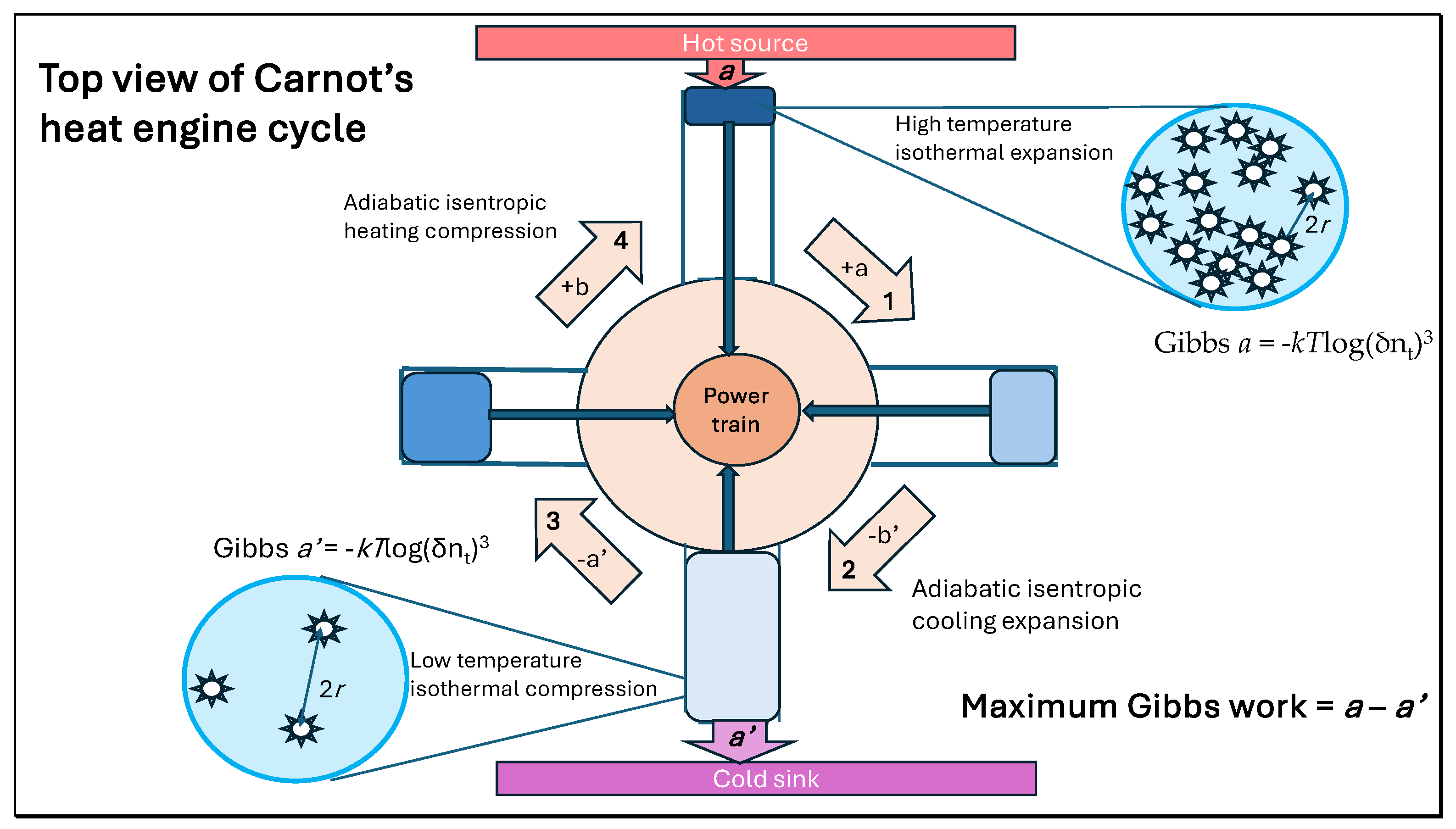
Figure 2. Proposed impulsive translational (A) and rotational (B) Gibbs quantum fields are shown for diatomic molecules such as N₂ and O₂. From Lagrangian variational theory the translational and rotation quantum fields are in opposition, quantum numbers increasing with altitude for translation but decreasing for rotation, with Gibbs energies increasing for both.

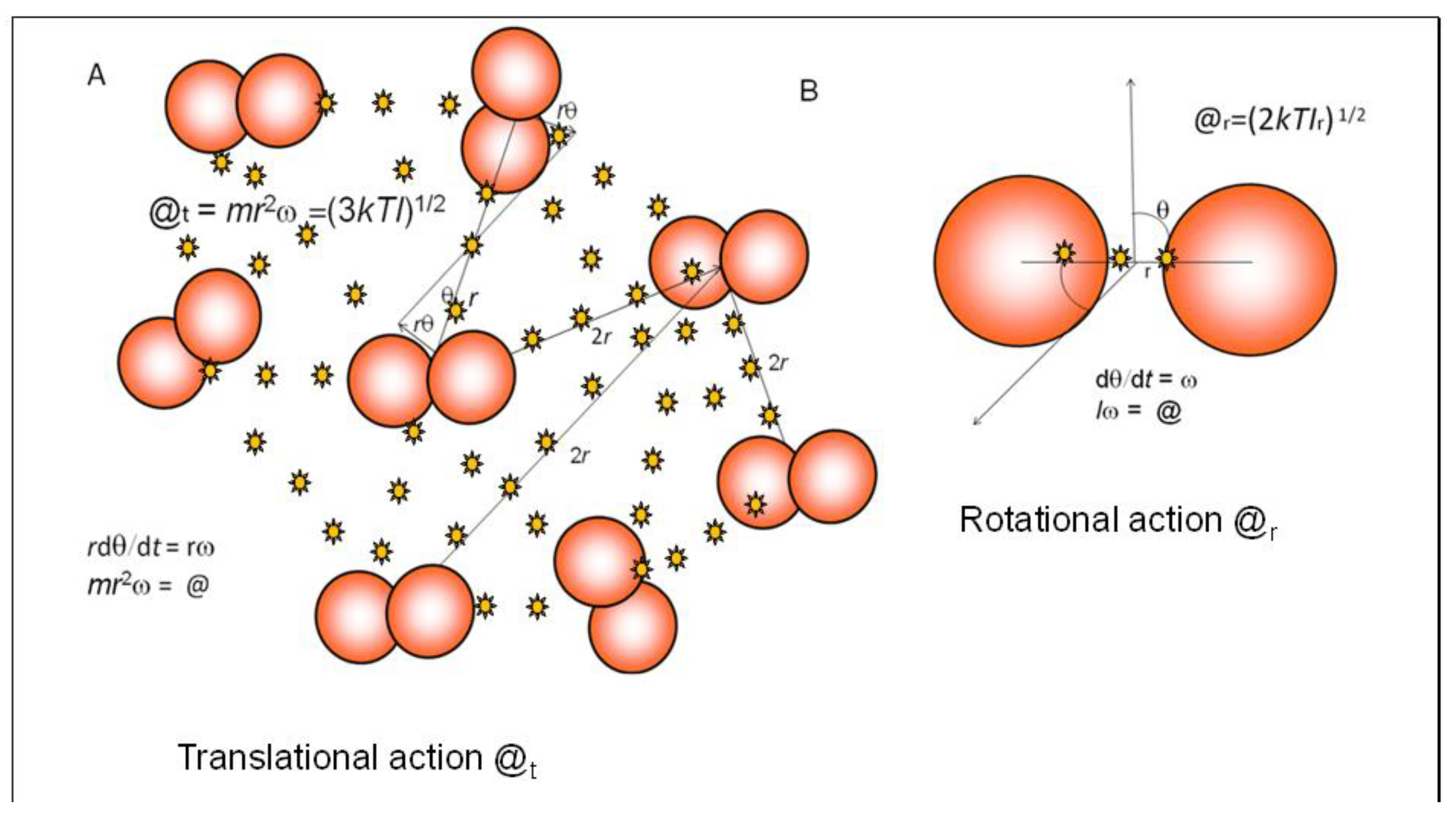
Figure 3. Variation in virial-action of half gravitational potential energy equated with kinetic energy is shown. Translational Gibbs field energy becomes available with altitude as temperature falls decreasing kinetic energy half the increase in gravitational potential. Translational and rotational Gibbs fields are in opposition, sustaining the configuration of the molecules rotating while translating. .

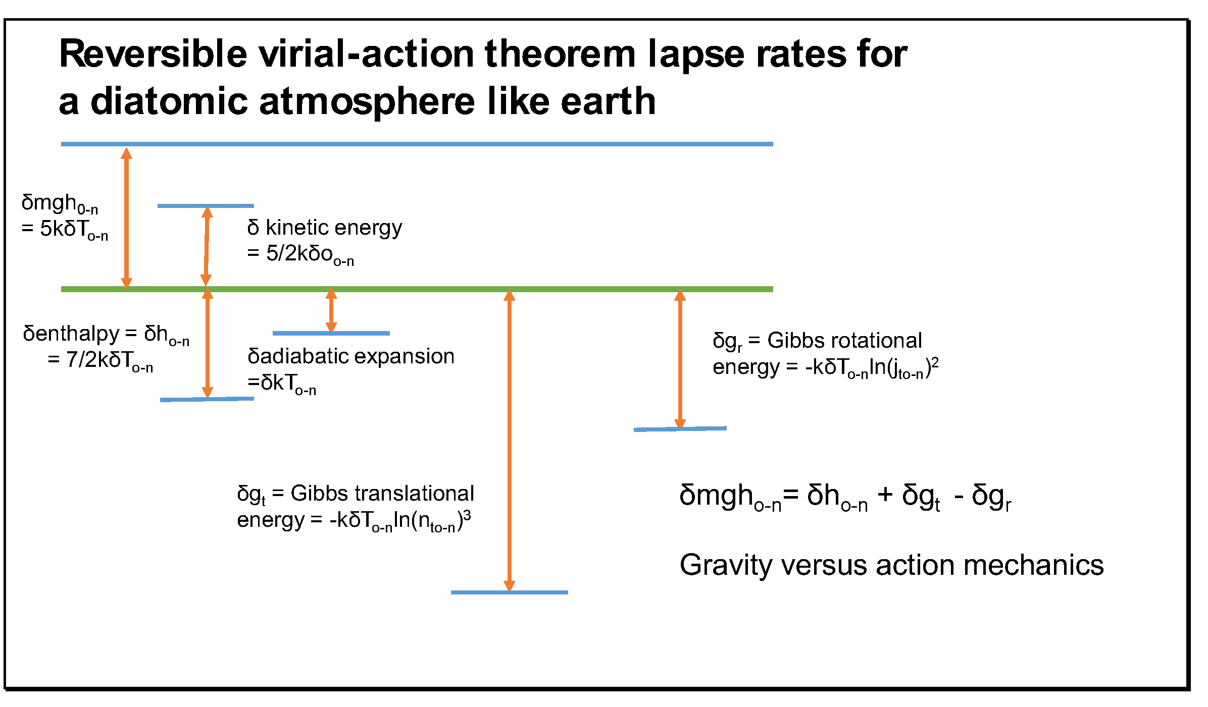
Figure 4. Cross section of a tropospheric cyclonic system for diatomic gases, with an ascending low pressure daytime central zone. After warming from absorption of sunlight at the surface, infrared radiation is then continuously emitted by a green surface as a hot source, partially recycled by greenhouse gas absorption (a). Internal work as convectional expansion (b’) against gravity cools air according to the virial-action theorem. Outgoing longwave radiation (Olr) passes high entropy heat to space as a cold sink (a’); gravitational compression and inertial surface motion compress air at the surface, reheating by turbulent surface friction, completing the multistage Carnot cycle (b).

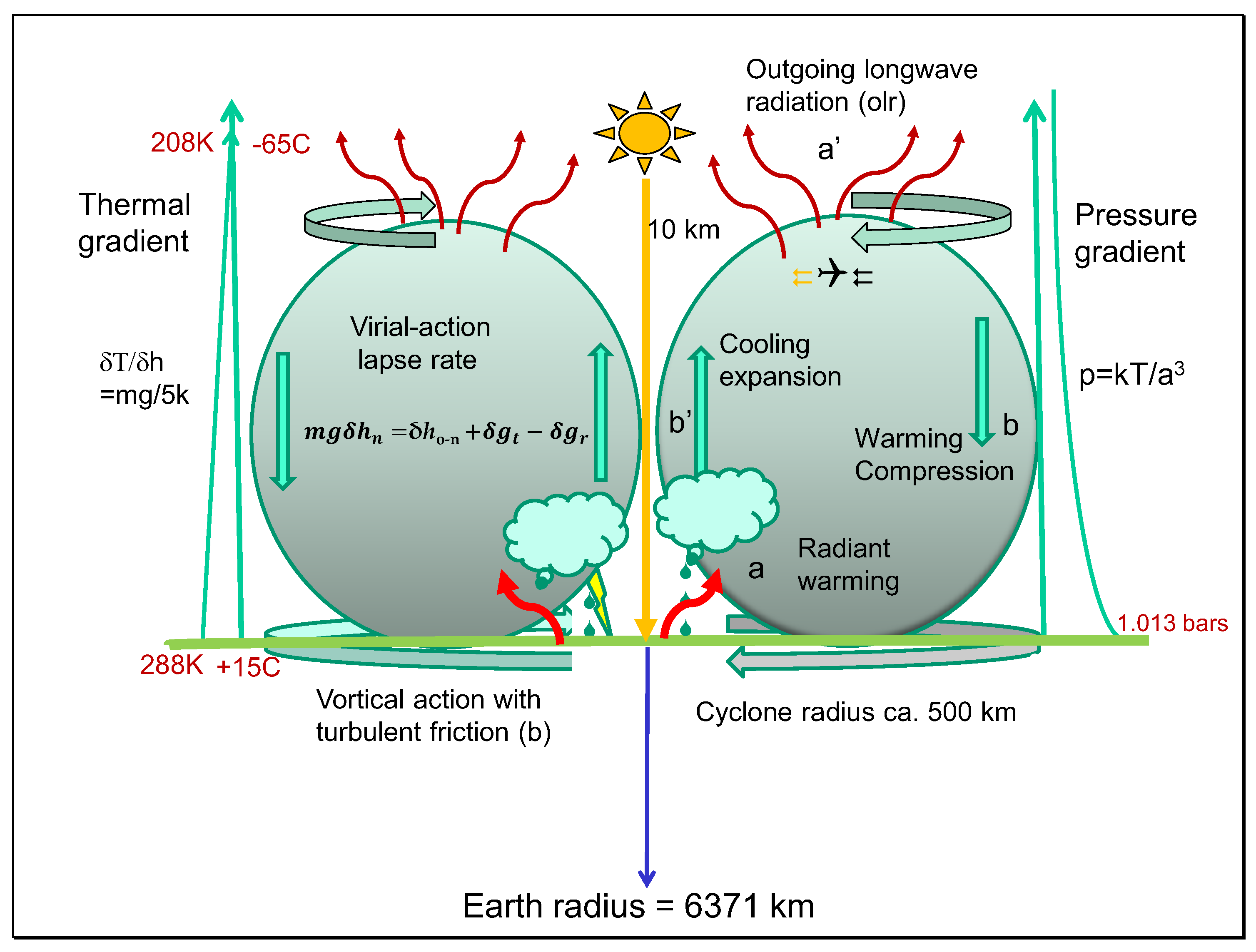
Figure 5. Flow diagram for computation in Astrocal of atmospheric profiles on Earth using inputs of molecular properties (mass, bond length, symmetry factors for translation and rotation, surface temperature and pressure, and altitude δh.

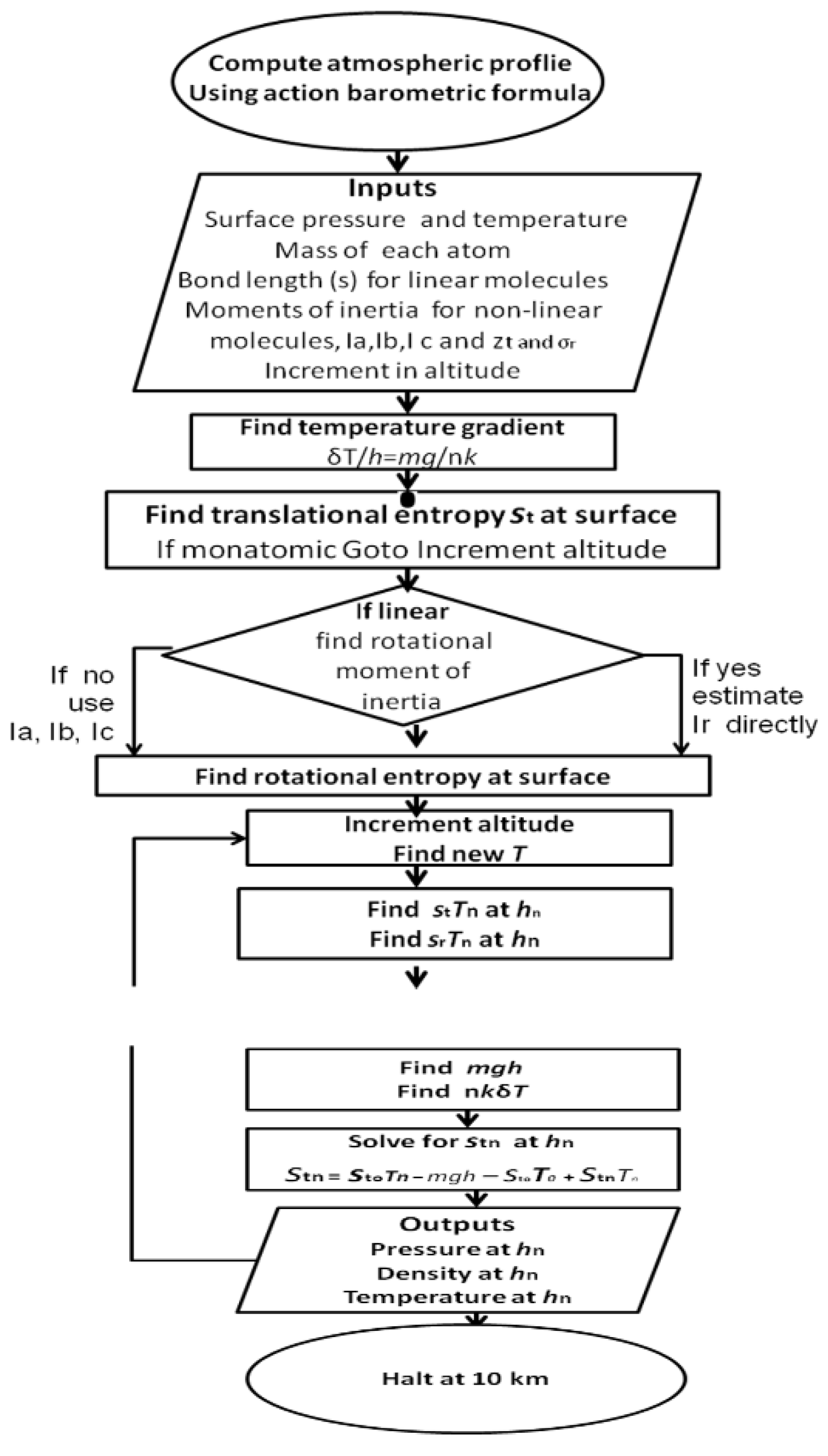
Figure 6. Comparison of atmospheric actual, virial and adiabatic lapse rates on planets and Titan. Data is extracted from Kennedy [15] and applies to values measured on the surface or close to 1 bar on the gas giants. Chi square statistical analysis shows the virial theorem lapse rate is decidely more consistent with observations than adiabatic lapse rates.

Figure 7. Comparisons of virial-action profiles for black body and greenhouse variation in temperature (K), negative Gibbs translational and rotational energy (x10²⁰ J) and pressure (bar) with altitude to 15 km in the Earth’s atmosphere.

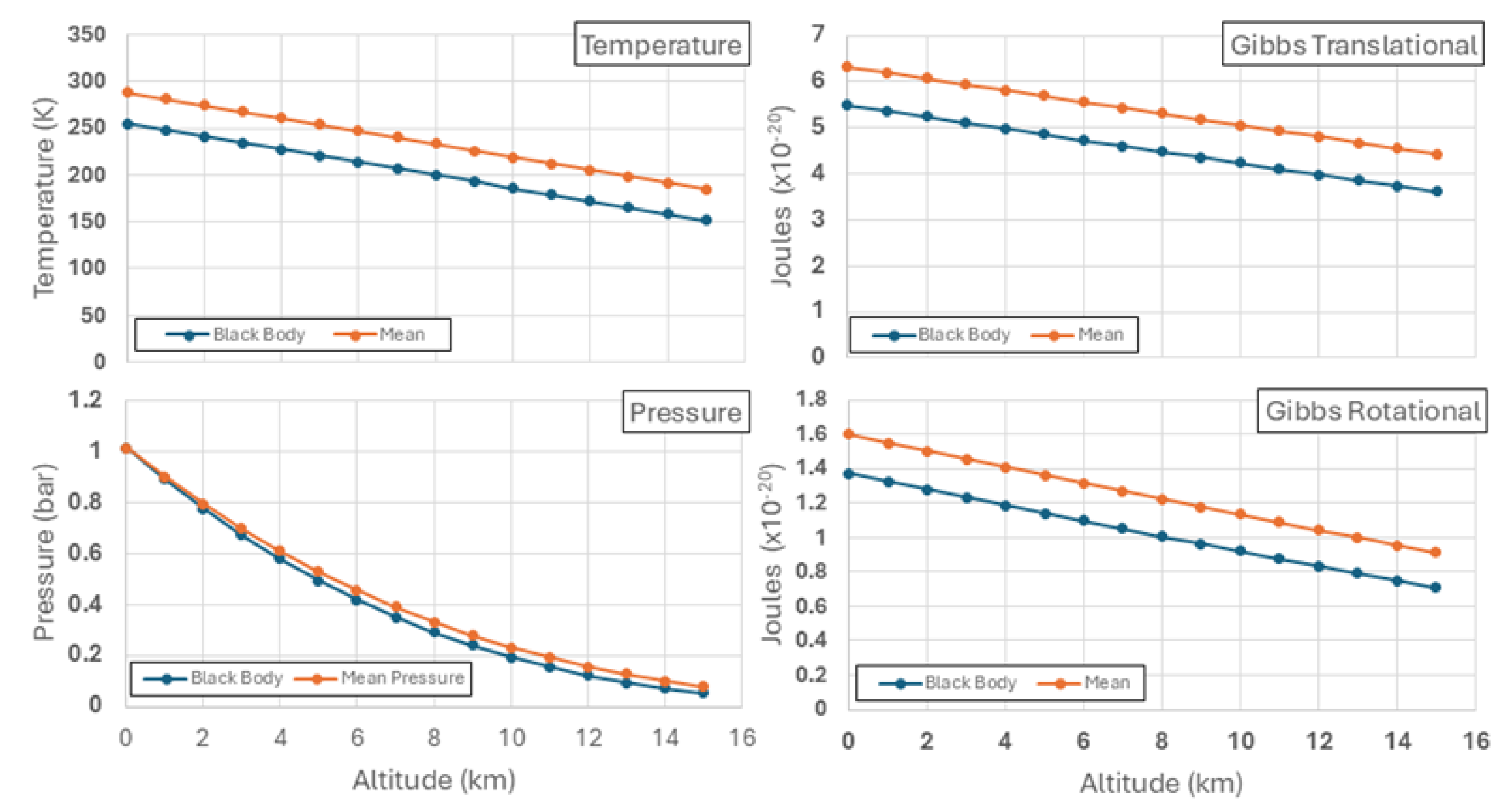
Figure 8. Comparison of surface to the tropopause altitude of Gibbs quantum fields and gravitational potentials for different latitudes. The virial-action profiles for Gibbs energies (x10²⁰ J) and gravity (x10^{22 J)} are plotted to the observed altitude at the tropopause, identified in Table 2.

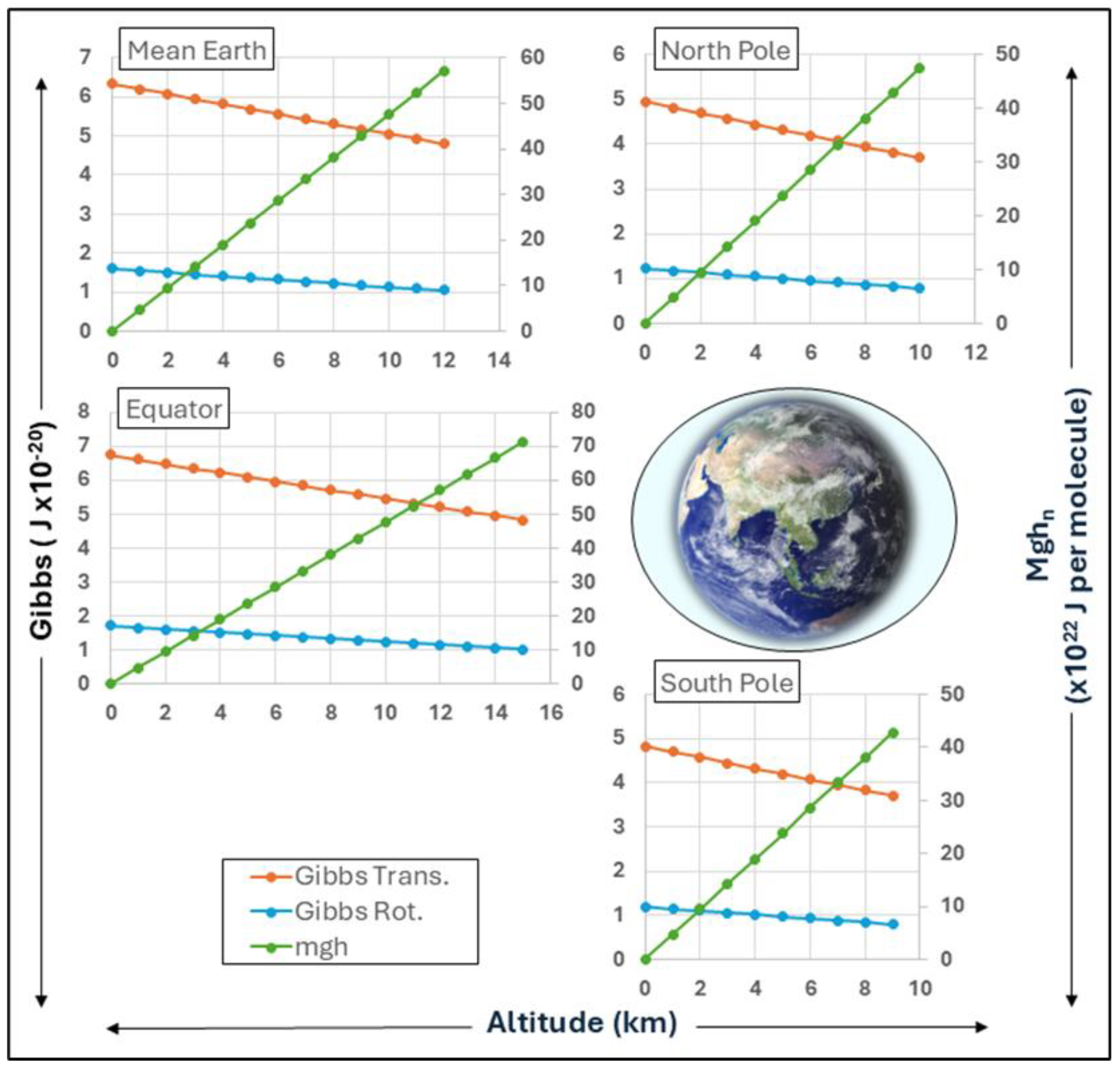
Figure 9. Southern hemisphere cross section of an anticyclone, showing a hot surface at the global mean 288 K (396 W/m²) powers vortical action and Gibbs energy, together with reversible virial-action gravitational work and heat releases. This cycle incorporates the Kiehl-Trenberth energy budget, including outgoing longwave radiation [21] shown as Olr, with 40 W/m² unimpeded by greenhouse gases.

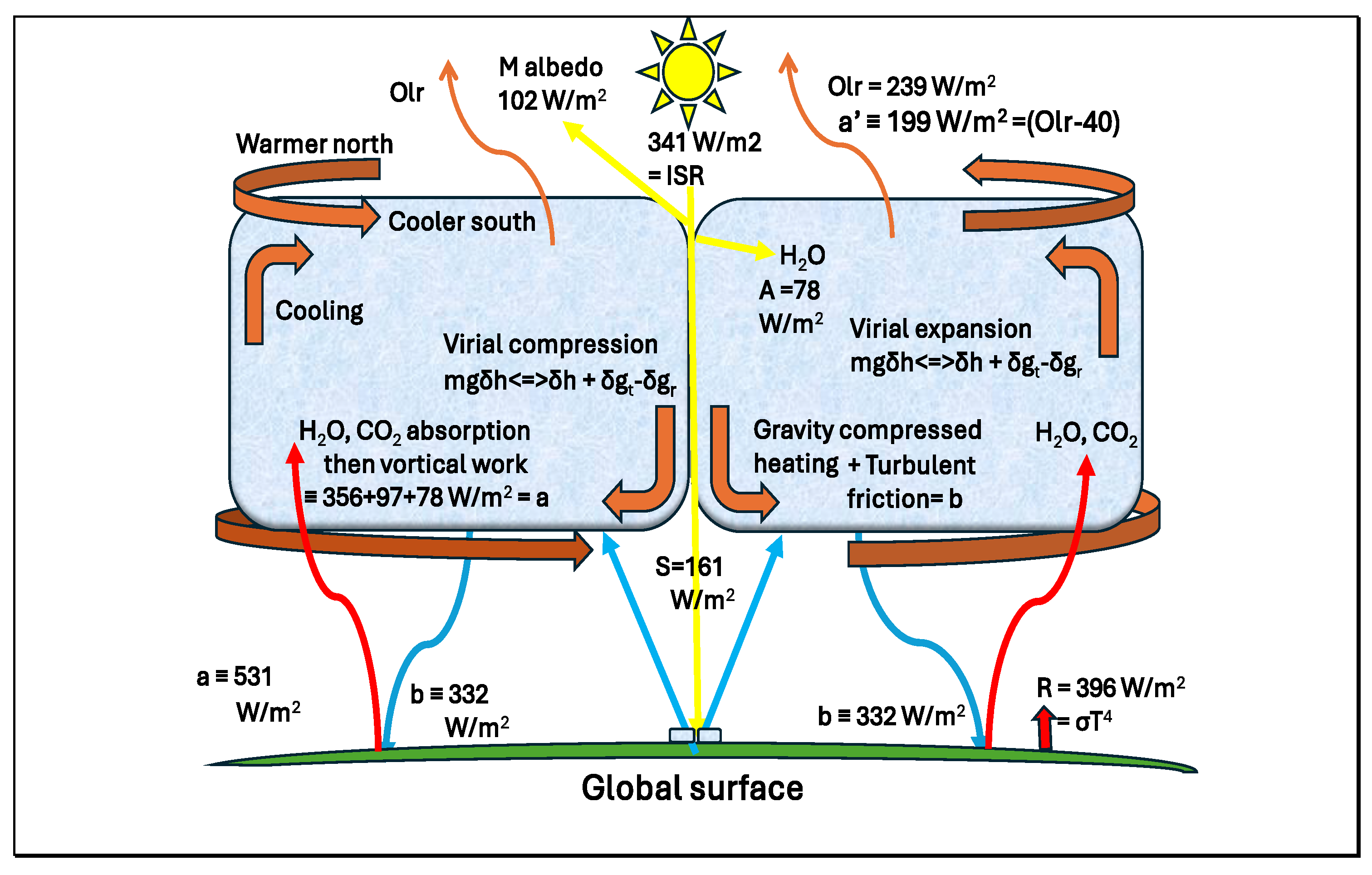
Table 4. Virial-action mechanics profile on Earth estimated for mean values of atmospheric molecules.

Altitude (km)	TempK	Estimate pressure x10^-5 Pascals	Estimate of density x10^-19 per cm³	Solved negative translational Gibbs energy kTln(n_t)³Q_e/z_t x10²⁰ J per molecule	Estimated from negative rotational Gibbs energy -g_{r =} kTln[(n_r)²/σ_r] x10²⁰ J per molecule	Temp K USAF	USAF Model 6 Pressure x10⁶ pascals
0	288.2	1.01282	2.545887	6.3252617	1.5965459	288.2	1.0130
1	281.3	0.89895	2.315004	6.1968176	1.5489674	281.7	0.8988
2	274.4	0.79384	2.095675	6.0686066	1.5016219	275.2	0.7950
3	267.5	0.69722	1.888033	5.9406345	1.4545154	266.7	0.7012
4	260.6	0.60880	1.692180	5.8129076	1.4076540	262.2	0.6166
5	253.7	0.52826	1.508188	5.6854323	1.3610441	255.7	0.5405
6	246.8	0.45527	1.336097	5.5582154	1.3146928	249.2	0.4722
7	239.9	0.38496	1.175904	5.4312642	1.2686071	242.7	0.4111
8	233.0	0.33059	1.027566	5.3045863	1.2227945	236.2	0.3565
9	226.1	0.27817	0.890993	5.1781896	1.1772636	229.7	0.3080
10	219.2	0.23187	0.766044	5.0520831	1.1320224	223.3	0.2650

Table 5. Variations in gravitational and thermodynamic properties with tropospheric altitude on Earth.

Altitude (km)	Estimated gravitational potential energy mgh_n x10²² J per molecule	Estimated decreasing enthalpy 3.5kδT=δh x10¹⁵ ergs per molecule	Estimated rotational Gibbs energy δ[kTln(n_r)²/σ_r] =-δg_r x10²² per molecule	Solved translational Gibbs energy δ[kTln(n_t)³/z_t] =-δg_tx10²² J per molecule	Solved cumulative translational Gibbs energy
0	0
1	4.75679	-3.32976	-4.75783	-12.84441	-12.84438
2	9.51359	-6.65951	-9.49241	-12.82111	-25.66551
3	14.27038	-9.98927	-14.20306	-12.79721	-38.46271
4	19.02718	-13.31903	-18.88920	-12.77269	-51.23541
5	23.78397	-16.64878	-23.55018	-12.74753	-63.98294
6	28.54077	-19.97854	-28.18532	-12.72169	-76.70463
7	33.29756	-23.30829	-32.79389	-12.69512	-89.39975
8	38.05436	-26.63805	-37.37514	-12.66779	-102.06754
9	42.81115	-29.96781	-41.92824	-12.63967	-114.70720
10	47.56795	-33.29756	-46.45235	-12.61065	-127.31787

The governing algorithm for diatomic or other linear molecules is that mgh_n-o + 3.5kδT_o-n = δ[kT_o-nln(n_t)³_o-n/z_t]. - δ[kT_o-nln(n_r)²_o-n/σ_r] = δg_t – δg_r;

Table 6. Profile conditions and Gibbs fields per molecule for tropospheric gases, including greenhouse gases.

Atmospheric gas	Temperature T	Density n/cm³	Pressure P	Translational -Gibbs field –g_t	Rotational Gibbs field -g_r	Vibrational Gibbs energy -g_c
	Kelvin	=1/a³	Dynes/ cm²	J/molecule	J/molecule	J/molecule
Water 0.0004 atm		x10^-15	x10^-2	x10²⁰ J	x10²⁰ J	x10²³
0 km	288.1500	10.1835493	4.0512848	9.016585189	2.07234140	1.24028461
5 km	270.3356	6.1502476	2.2954659	8.611636060	1.90849468	0.72861960
Water 0.016 atm		x10^-17	x10^-4	x10²⁰ J	x10²⁰ J	x10²³
0 km	288.1500	4.07341976	1.6205139	7.549051568	2.072341403	1.24028461
5 km	270.3356	3.13706846	1.1708526	7.144102429	1.908494677	0.72861960
CO₂ 0.0004 atm		x10^-15	x10^-2	x10²⁰	x10²⁰	x10²¹
0 km	288.1500	10.1835494	4.0512848	9.549961720	2.24865929	1.79371631
5 km	239.6064	0.87391569	0.2890965	8.661879002	1.80880709	0.62083771
N₂ 0.78 atm		x10^-19	x10^-5	x10²⁰	x10²⁰	x10²⁵
0 km	288.1500	1.98579213	7.9000053	6.266476733	1.561650059	3.89511735
5 km	254.8849	1.20911641	4.2548799	5.652889568	1.338200586	0.82971538
O₂ 0.21 atm		x10^-18	x10^-5	x10²⁰	x10²⁰	x10²³
0 km	288.1500	5.34636343	2.1269245	7.30523956	1.69715480	1.32545576
5 km	250.1497	2.09532214	0.7236454	6.59208978	1.42449783	0.39379343
Argon 0.01 atm		x10^-17	x10^-4	x10¹³
0 km	288.1500	2.5458873	1.0128212	8.21253258	0	0
5 km	250.1497	2.09532214	0.7236454	6.59208978	0	0
N₂+O₂+Ar 1.0 atm		x10¹⁹	x10⁵	x10²⁰	x10²⁰
0 km	288.150	2.54588734	10.128212	6.324644044	1.596607545	negligible
5 km	253.7317	1.50945891	5.287750	5.685466013	1.361338787

Disclaimer/Publisher’s Note: The statements, opinions and data contained in all publications are solely those of the individual author(s) and contributor(s) and not of MDPI and/or the editor(s). MDPI and/or the editor(s) disclaim responsibility for any injury to people or property resulting from any ideas, methods, instructions or products referred to in the content.

© 2024 by the authors. Licensee MDPI, Basel, Switzerland. This article is an open access article distributed under the terms and conditions of the Creative Commons Attribution (CC BY) license (http://creativecommons.org/licenses/by/4.0/).

Copyright: This open access article is published under a Creative Commons CC BY 4.0 license, which permit the free download, distribution, and reuse, provided that the author and preprint are cited in any reuse.

Downloads

Views

Comments

Subscription

Notify me about updates to this article or when a peer-reviewed version is published.

MDPI Initiatives

Important Links

Choose an area of interest and we will send you notifications of new preprints at your preferred frequency.

Disclaimer