Using Random Forest for Delineation of Dimension Stone Qarries. Mapping of the Santa Eulália Plutonic Complex (Portugal)

The Santa Eulália Plutonic Complex is a large granitoid ring-complex exhibiting several granite facies, gabbro-diorite rocks and roof pendants from the country rocks. This lithologic variability crossed with the spatial distribution of each lithotype within the complex enables the grouping of the different magmatic rocks in: G0 group (“pink-reddish” granites in an external belt), G1 group ("greyish” granites in the inner part”) and M group (gabbro and diorite as enclaves in the eastern regions of the G0 group). All these groups host facies of interest for dimension stones due to their aesthetic value and, therefore, a systematic thematic mapping has been conducted and refined throughout the years. In this work we verify the applicability of Sentinel-2 multispectral images combined with Random Forest as a classification methodology to distinguish the different gran-itoid groups and support large-scale lithological mapping. The results show overall accurate outline of the facies, with areas corresponding to the G0 group displaying good predictions, areas representing the G1 group moderately good predictions, and areas established for the M group poor predictions, obtaining Producer’s accuracies of ~82%, ~60%, and ~30%, respectively.

Keywords:

Santa Eulália Plutonic Complex

;

Machine Learning

;

Random Forest

;

Dimension Stone

;

Red Granites

;

Grey Granites

;

Gabbro-diorite

;

Sentinel-2 L2A

Subject:

Environmental and Earth Sciences - Remote Sensing

Supplementary Material

supplementary.pdf (30.75MB )

1. Introduction

Dimension stones, i.e., natural rocks susceptible of being quarried with the purpose of producing a variety of construction and decorative materials with appropriate extent and shape, need to correspond to rigorous criteria that include size, durability, strength, resistance to polishing and final aesthetic features (e.g., [1]).

Granites are commonly found worldwide with a large variety of textures that makes them a preferred raw material for being quarried. In particular, coarse and medium grained granites are prone to be polished by cost-efficient techniques, and the variety of colours (that necessarily depends on the mineralogical attributes) give them added visual value. The quality of granites used for architectural purposes plays an important role in its valorisation as a dimensional stone, however, the availability of exploitable types according to the global market demands may be challenging, either by the absence of the specified dimension stones in the region or by the lack of knowledge of the resources.

Thematic geological mapping is thus an indispensable step in the characterization of resources, as it should integrate the most important information, such as the identification (e.g., textural variety or different rock types), assess the quality and delimit the structural geometry of the target stone. This is especially important when considering coloured granites that are rather uncommon, such as the reddish and dark coloured (more valorised as ornamental stones), when compared to the typical grey varieties.

In Portugal, granite quarrying is a common practice but there are few exploitation centres that host reddish granites and other darker granitoid stones [2]. Therefore, achieving proper delineation of the extent of such uncommon rocks in areas where outcrops are scarce, near the limits, or where knowledge about the internal structure of the massif is low, could benefit from novel approaches (like Machine Learning and Artificial Intelligence methods) to ensure the stone continuity, which would then be useful for resource valorisation and support industry exploiting these types of stones.

In this work, we propose the use of Random Forest, a supervised Machine Learning (ML) method for classification that has proved to be reliable for thematic mapping, e.g., [3,4,5], as a first approach to attempt to determine distinct types of magmatic rocks (diverse types of “pinkish/reddish” and “greyish” granites, as much as gabbro-diorite rocks) that embody the Santa Eulália Plutonic Complex (SEPC). All the different magmatic facies of the SEPC have been exploited to some extent; nowadays there are fewer exploitations, most of them for ornamental stones, but also for aggregates. This activity left several exposed quarry sites, visible from satellite. Therefore, the SEPC is an excellent work-case scenario to test and apply the ML methods as a support for geological mapping in this context.

2. Regional Framework

2.1. Geodynamic Setting

The Iberian Massif is the southwestern segment of the European Variscan Belt, and comprises the structures emplaced during the Palaeozoic opening and closure of the Rheic Ocean, followed by the continental collision that formed Pangea - also referred to as the Variscan Wilson Cyle (e.g., [6]). The major stages of the Iberian Massif are the Cambrian-Ordovician rifting processes, with marine sedimentation overlaying previous Ediacaran formations and rift-related volcanism (e.g., [7]), followed by the Ordovician-Lower Devonian drifting phase (e.g., [8]), and finally the mid-Devonian subduction and continental collision processes, majorly represented by large magmatism that persisted until Permo-Carboniferous times ([6,9]). The processes related with the compressive phases imposed a tectono-stratigraphic zonation throughout the Iberian Massif, with different tectono-magmatic and metamorphic characteristics according to distance from the Rheic suture zone (e.g., [10]).

The Ossa-Morena Zone (OMZ), located north of the suture zone (in the southern region of the Iberian Massif), hosts several collision-related magmatic bodies. Large intrusions, mostly Middle Mississippian-Lower Pennsylvanian in age, outcrop in the OMZ western and southern borders: the Veiros, Vale de Maceiras and Campo Maior gabbroic plutons [11,12,13], the Beja Igneous Complex gabbroic rocks and the Évora Massif granitoids [9,14,15,16]. Post-kinematic granitoid bodies are less common and mostly occur on the northern and central regions of the OMZ during Upper Pennsylvanian-Cisuralian, such as the Ervedal, Fronteira and Elvas granites, and the large Santa Eulália Plutonic Complex (SEPC; [17,18,19,20,21]). All these lithological units of the Iberian Massif reflect the continental collision effects, that are translated by NNE-SSW and E-W brittle to brittle-ductile strike-slip faults, well expressed in local and regional fracturing patterns (referred as the late-Variscan deformation event [22]).

The SEPC spawns in the northern OMZ region (Figure 1) along with other collision-related stocks, cutting the Ediacaran-Cambrian metasedimentary rocks and rift-related magmatic bodies that occur in the Alter do Chão-Elvas Sector (at southwest) and the Tomar-Badajoz-Córdoba Shear Zone (in the northeast).

2.2. The Geology of the Santa Eulália Plutonic Complex

The SEPC is a granitoid ring-complex emplaced in the northern Ossa-Morena Zone region, as mentioned. It is a late- to post-Variscan magmatic batholith (area ≈ 400 km²) with an ellipsoidal W-E major axis shape that crosscuts the previous pre-collisional NW-SE trending structures from Ediacaran-Cambrian times (c.f. Figure 1). This sub-circular complex consists of an assemblage of intrusive units (ranging from several granite facies to diorite and gabbro) with metasedimentary enclaves that can be correlated with the country rocks. A mappable lithological discernment has been assumed, separating an inner unit of “greyish” granites (informally designated as G1 group), from an external ring of “pink-reddish” granites (G0 group) that envelop numerous enclaves of a diorite and gabbro rocks (M group) and country rocks xenoliths [18,21,24].

Granite facies from both the G1 and G0 groups have been further subdivided in three major zones each based on textural varieties (grain size and colour) that implicate the aesthetic interest for the industry (Figure 2). Likewise, the G1 group is divided in three concentrical belts of grey granite facies with coarse (G1 facies), medium (G2 facies) and fine grain size (G3 facies) changing respectively from the outer to the central, and the G0 group in three areas of distinct fabric around the massif that go from “coarse-grained pink to red” (in the west), “coarse-grained grey to pink” (in the northeast) and “coarse-grained pink to red” (in the southeast) granites. Despite all the divisions, there are authors that further subdivide each of the G0 group facies in smaller patches of the same unit but with a slight variety on the grain size and shade [2,24].

Works regarding the fracturing pattern of the SEPC showed two major directions of sub-vertical to vertical joints (N30° - N45° and N90° - N115°) [26,27] congruent with the patterns of the late Variscan deformation event [22]. The major directions cut all the facies, though structures ranging N320°- N330° derived from late-magmatic and magmatic-hydrothermal processes, especially evidenced in the G1 group area (quartz lodes, veins and greisen structures [28,29].

The inner region of the SEPC is characterized by a typical granite landscape (Figure 3) of whitish-grey granites from the G1 group, commonly outcropping as boulders or rounded blocks, and often forming tors. The outcrops show some particular features such as the development of micaceous schlieren (e.g., Figure 3b) and delta structures indicative of ascending melt flow (compatible with magnetic lineaments published in literature [19]). Gravimetric data show a thick continuity beneath the surface and the probable deep crustal G1 group melt origin, towards east [19,21]. Zircon U-Pb radiometric data provided a consistent crystallization age of 302 ± 2 Ma [25] for the rocks of this group. Despite the limits shown in the available regional geological maps found in literature [2,18,21,24], the spatial relationship between the G1 group and rest of the SEPC is still not well defined.

Contrastingly, the external ring is extremely heterogenous regarding its lithological units. Not only granites from the G0 group outcrop with the most notorious textural variation throughout the region (Figure 4), but also the hosted enclave type varies from gabbro-diorite masses to country rocks xenoliths according to the segment they occur, with an apparent constraint regarding the host G0 facies (Figure 2).

In the western segment, the medium-grained “pink to red” granite is the prevalent facies (Figure 4b), covering the largest area. The presence of xenoliths is very common in this part, either as small irregular enclaves within the granite or as large blocks of country rocks sequences affected by contact metamorphism, mostly hornfels and calc-silicate rocks [30,31,32] geometrically disposed as metasedimentary roof pendants above the western granite facies (Figure 4d). The roof pendants comprise rocks from at least four lithostratigraphic units, namely the Ediacaran and Cambrian schistose formations, the Carbonate Formation, a quartzite bar, and meta-mafic rocks. Enclaves of M group rocks are rarer in this part of the SEPC.

In the northeastern region granites are coarse-grained and have a “pink-greyish” colour (Figure 4c). Despite the common occurrence of xenoliths as small mesoscale enclaves, no roof pendants have been mapped in this area. However, large sites of M group rocks have been delimited as the only macroscale enclaves for this segment.

The southeastern most part of the SEPC is dominated by coarse-grained “pink to red” granite and is the only facies of the G0 group spatially associated with both enclaves of the gabbro-diorite M group and with roof pendant xenoliths.

The increase of the reddish intensity on all granite facies from the G0 group is assumed to be due to the impregnation of iron oxides in feldspars [2] which provide textural aspect that range from Figure 4c to the granite aspect from Figure 4b.

The “pink-reddish” granites of the SEPC have been dated with zircon U-Pb radiometric methods which yielded crystallization ages of 297 ± 4 Ma [20], and 301 ± 0.9 Ma [25], as well as Rb-Sr isochron of mica concentrates that indicate an age of 290 ± 5 Ma [17].

The gabbro-diorite rocks from the M group outcrop as minor masses and lenses within the northern and eastern segments of the external aureole. The limit between rocks from the M group and the G0 granites rarely outcrops, and is characterized by a sharp contact, with apparent emplacement of the granites over the gabbro (Figure 5a). The gabbro-diorite association commonly shows complex magmatic structures of mingling and mixing/unmixing, suggesting different coexisting melts that formed either by different magma injection events, replenishment, or by immiscibility (Figure 5b,c). Available geochronological data determined 303 ± 3 Ma [20] and 307 ± 2.5 Ma [25] zircon U-Pb ages for these rocks.

The close overlapping ages determined for the rocks of the SEPC and the contrasting geochemical and petrographic features found especially between the G1 and G0 groups induced a debate regarding their nature and genetic association that still remains open, of either the G0 and G1 derived from a primeval melt, or there are distinct sources of liquid. In any case the M group rocks are considered as autoliths present in the external facies. But regardless the interpretation of petrogenesis, and independently of the origin and contemporaneity of the melts that gave origin to these rocks, the SEPC consists of an important target for dimension stone exploitation, and all granite and gabbro facies have been exploited to some extent in the past. A list of exploitable facies of the SEPC can be found in Table 1.

3. Methodology: Random Forest as a Mapping Tool

Sentinel-2 images of the SEPC are used to apply the supervised ML algorithms to aid lithological mapping of the different groups; this work is the first approach proposed to automatically delineate the broader extent of the facies. Figure 6 entails the summary workflow from data acquisition to the resulting thematic maps. Additionally, an Exploratory Data Analysis (EDA) was performed on all datasets before the Random Forest modelling, assessing data balance, descriptive statistics, and band correlations.

The images were obtained from the Copernicus Browser [34], as L2A processing level image – i.e., an orthorectified, atmospherically corrected image in surface reflectance – the date of acquisition is the 2nd of August of 2023, a yearly period that contains a low presence of vegetation, and a cloud coverage of ~1%. A total of 12 bands were processed, but band 1 was excluded from ML processing because it is mainly associated with atmospheric factors, and thus considered not of interest for this study.

To prepare the data for classification algorithms, the bands were resampled to 10 m using the nearest neighbour method and cropped accordingly to a SEPC groups shapefile (Figure 2), excluding the roof pendants. To accurately classify bare soil and outcropping rocks, the image was masked using the Normalized Difference Vegetation Index (NDVI, Equation (1)), the Normalized Difference Water Index (NDWI, Equation (2)), OpenStreetMap information [35], and Corine Land Cover 2018 [36], to respectively identify and remove vegetation, water features, paved roads, and urban centres.

NDVI = (B8 – B4) / (B8 + B4),

(1)

NDWI = (B3 – B8) / (B3 + B8).

(2)

For this work, sections of exposed rocks and soils were defined representing all the lithological groups (i.e., the G0, G1, and M groups), maintaining the frequency proportion of the different groups (Figure 7). The pixel value of the bands and lithology information were extracted and used to create the datasets used in the ML classification models: i) Complete (full satellite after masking processes) and ii) Subset (containing only information regarding the sectioned areas of Figure 7). Additionally, data was extracted prior to masking pre-processing step for EDA comparison (original data). Random Forest (RF) is a supervised classification ML algorithm that uses labelled information, to assist in the construction of a predictive model to do lithological classification within the SEPC. RF is based on an ensemble of Decision Trees, categorizing data according to the variables used for training, i.e., the spectral bands [37]. Due to its ability to use multiple variables and resistance to overfitting, it is widely used in Remote Sensing studies, achieving good accurate results (up to 91%) [5,38,39]. The models trained with Complete and Subset datasets used the SEPC groups as labels and the bands 2 to 12 as training variables. In both instances the data was split into ‘training’ and ‘testing’, necessary to validate model performance and accuracy. Train stratified datasets of 10%, 30%, 50%, 70% and 90% were created, allowing for accuracy calibration; model parameters were set to an optimized number of variables randomly sampled as candidates at each split (mtry parameter), with respect to an optimized Out-of-Bag error estimate, and a forest of 250 trees (ntree parameter). The models were created using a custom script in R [40].

The 10 trained models (from 10% to 90% training sample size, Complete and Subset datasets) were used to predict the main lithological groups of the SEPC. Validation metrics such as confusion matrix, overall accuracy (OA), user’s accuracy (UA), producer’s accuracy (PA), and Kappa coefficient are used to quantify the model performance in both test and SEPC predictions. OA represents the proportion of correctly classified pixels, without discriminating any class, as opposed to UA and PA which represent class-wide from the point of view of the map user, or the map maker, respectively: UA informs on much each prediction correctly identified the class label while PA relates to how each label is correctly classified. Kappa coefficient [41] informs on how well the classification is compared to randomly assigning classes to each pixel, by confronting the predictions to randomly assigned values, ranking the coefficient between -1 (totally random) to 1 (perfect prediction). Lastly, the predictions are rasterized for visual assessment and data interpretation.

3. Results

This chapter presents the EDA and the RF modelling results, divided by the datasets. The latter is further sectioned by the two model predictions, firstly to the Test dataset, and then to the SEPC. In both instances, the models were subjected to the performance metrics, namely confusion matrices (see supplementary materials), accuracy (overall, producer’s, and user’s), and Kappa coefficient, proceeded by data rasterization as final output.

3.1. Exploratory Data Analysis (EDA)

3.1.1. SEPC Lithological Atlas

EDA is essential to assess data balance and band correlation, providing a strong support for data validation claims. A better understanding of the Subset areas can be achieved through characterization of each component, including the spectral signatures, for each group. Figure 8 contains areas representative of each lithology (for complete list, see supplementary materials). Here, the masking process of removing vegetation, water and roads/ cities are filled with white pixels (Masked). Corine Land Cover (CLC18) reveals no relation between land cover uses and the lithotypes, and as such it was only used to identify and remove the urban fabric (not represented here). Likewise, the spectral signatures (SS) do not reveal any clear difference between the groups.

3.1.2. Descriptive Statistics

A comparison of the results between the two datasets (Complete and Subset) to the dataset before masking the pixels (Original data) was made, assessing for pixel proportion (and respective frequency) (Table 2), and correlation matrices (Figure 9). Lastly, Table 3 indicates the minimum, median, and maximum values of each band, grouped by dataset.

Table 2 shows that G0 is the largest group across all groups, representing ~57% of the total number of pixels, followed by G1 group, averaging ~37%; M group has a small representation, with less than 6% average. Across datasets, the difference between the groups is smaller than 3%, indicating that group frequency and proportion is maintained.

Based on the correlation matrices, four band groups can be distinguished, common in all datsets: i) B1 is always a separated group, ii) Bands 2 to 5, representing visible and very near infrared (VNIR), iii) Bands 6 to 9, representing near (NIR) to shortwave infrared (SWIR), and iv) Bands 11 and 12, representing the higher SWIR wavelenghts.

3.2. Complete Dataset Models

3.2.1. Complete Testing Sets Predictions

The testing dataset predictions are fundamental to prevent overfitting and provide a general assessment to model performance. Confusion matrices were produced, which compare the classed labels to the predicted outcome, and allow for the extraction of OA, UA and PA, that validate the model along with the Kappa coefficient (Table 4).

Table 4 reveals a positive correlation between the percentage of training data used and the validation metrics, with Kappa coefficient classifying these predictions as moderate (10%, 30%, and 50% training sample sizes) to substantial (70% and 90% training sample sizes) according to [41] proposed scale. At 10% the UA is approximately the same as the OA, but has a higher growth rate, attributed to the M group, with more correct predictions than G0 and G1 groups (Figure 10a, see supplementary materials for individual accuracy classes for each model), albeit only reaching “good prediction” results. PA shows the lowest scores off all accuracy metrics, attributed to the poor (10%) to moderately poor (30%, 50%, and 70%) M group percentages (Figure 10b). However, the PA’s increased growth is also attributed to the same group, as G0 and G1 have a less steep growth incline.

3.1.2. Complete SEPC Group Predictions

The models were used to predict the SEPC, i.e., the Complete dataset before splitting into train and testing datasets (Table 5). OA shows good predictions, increasing from 75,94% to almost perfect at 98,33% accuracy. UA’s lowest accuracy is ~75%, by G0 group (with 10% training sample size), closely followed by G1 group, and then M group (Figure 11a). As the training sample size increases, the difference between the three groups is reduced, with all three having very good to perfect UA predictions. PA is the lowest accuracy metric, with a more pronounced difference in the 10% and 30% training sample sizes, attributed by the M group (Figure 11b). The Kappa coefficient values show a great increase in model confidence, from moderate (10%), substantial (30% and 50%) to almost perfect (70% and 90%).

The UA and PA for both testing and SEPC group set predictions reveal that the M group has greater UA scores and lower PA scores than the other groups. This is indicative of a large number of M group predictions matching the real M group labels, but for a small number of M group pixels accurately predicted as such.

3.3. Subset Dataset Models

3.3.1. Subset Testing Sets Predictions

As with the Complete dataset, the Subset models were used to predict a test dataset, essential for data validation and to provide an assessment on model performance, including the calculation of accuracy and Kappa coefficient metrics (Table 6).

Table 6 shows an increase in all accuracy and Kappa coefficient values, as the percentage of data used to train the models is increased. UA is higher than OA, due to the very good classification of M group rocks, ranging from 81 to 93% (Figure 12a), while G0 and G1 rocks share approximately the same percentage as the OA. PA increase in the different models can be attributed to the larger correct number of pixels in the M group, from 44.32% in the 10% Model, to 73.53% in the 90% Model (Figure 12b). The G0 shows the smallest growth, with an average increase in accuracy of 1.68% in each step. However, this group’s predictions are the closest to a near perfect prediction record.

The Kappa coefficient is between 0.52 and 0.74, classified as moderate (10 and 30% models) to substantial (50, 70, and 90% models).

3.2.2. Subset SEPC Group Predictions

Following model validation by the test dataset, the predictions on the study area was performed, classifying the soil and rock pixels of the SEPC as either G0, G1, or M group rocks.

Table 7 indicates a moderate OA ranging between 67.95 and 70.84%, with a poorer performance than test dataset. Kappa coefficient is also lower, classified as fair (10 and 30% models) to moderate (50, 70, and 90% models). Both UA and PA steadily increase, albeit with at a slower rate compared to the test dataset. Contrarily to the test dataset, the UA value for M group is consistently low, between 38% and 45%, balanced by the G0 and G1 group classifications, that are ~70% across all models (Figure 13a). The PA shows very good classifications on G0 group (~81%), moderately good classifications for G1 group (~58%), and poor to moderately poor for M group (~27%), showing the variable difficulty in classifying and identifying the different groups (Figure 13b).

Comparing both testing and SEPC group set predictions, the observed behaviour for G0 and G1 is the same, with approximately equal UA percentages, and PA values that grow approximately at the same rate. However, it is noteworthy that while M group’s behaviour for the Testing set is like the one encountered in the Complete model predictions, the same is not found when predicting the SEPC, and the UA is far below the remaining groups.

For the SEPC group sets, the predictions were rasterized into thematic maps following the new classifications (Figure 14a,b, see supplementary materials for all figures). Based on the total number of pixels used in training and predicting the SEPC groups, the Subset model with 90% training size sample (which equates to approximately 11.93% of the total number of pixels in the SEPC) was compared to the Complete model with 10% training sample size, allowing to match pixels with the same classification predicted (coloured by respective group colour) and those that do not match (coloured in blue) (Figure 14c). This last figure is also overlayed by the geological map, informing which regions were misclassified.

4. Discussion

This work explores an established workflow for remote sensing data classification [38,39], including the removal of vegetation, water bodies, urban centres and roads. The RF algorithm trained two models (Complete and Subset datasets), with 10%, 30%, 50%, 70%, and 90% of data, used to predict the test and the SEPC groups. Results were validated using confusion matrices, supported with accuracy and Kappa coefficient metrics.

4.1. Test Dataset

The test dataset was used to verify the validity of the trained models, using the remainder of the data that was not used for training. The results indicate a good overall accuracy, without reaching perfect predictions, inferring a well-trained model without overfitting. Furthermore, the high UA percentage indicates good reliability on the predicted classifications, as they are mostly correctly classifying the real features. This is especially visible for the M group, where the UA is at least 5% higher than the other classes and reaches 95.70% on the 90% model. It is noteworthy that most of the incorrectly identified M group classifications fall within the G0 group, that envelop these rocks. The PA reveals that G0 group, the pink-reddish granite, are the best classified rocks in the test dataset, with an accuracy above 86%. Conversely, the M group shows low PA, detailing that most of the M group is not classified as such. However, this is also the group with the highest increase in accuracy as the train set is increased, showing how important it is to use a minimum quantity of pixels for each class to be correctly classified. As such, the differences in UA and PA for the train dataset can be used to infer that the G0 and G1 groups are either relatively homogeneous on their respective spectral signature, or that their intra-variational differences are sufficiently well represented within the confines of the chosen training areas. This does not seem to be true for the M group rocks, requiring a larger sample size to be correctly classified, as observed for the 50%, 70%, and 90% models. This group is composed by a mix of gabbro-diorite rocks, and as the diorites are usually found as masses at outcrop scale, is unlikely to interfere with the spectral signature.

4.2. SEPC Dataset

The main interest in training the models was to assess how well the RF classification algorithm could classify the SEPC groups using regions of training. The performance metrics indicate an overall moderate performance in accuracy, slightly increasing as a larger sample size is used. The average UA is lower than the average OA, but in individual accuracies, both G0 and G1 groups share approximately the same percentage than the OA, and the M group unit is responsible for the lower UA, contrarily to the observed dataset predictions.

The individual assessment of the classes for PA clearly shows that G0 predictions mostly correctly classify G0 areas mapped in the geological maps, moderately predicted the G1 group, and have a poor performance classifying the actual M group. Furthermore, both UA and PA have only a small increment of accuracy when increasing model percentage, indicating that the models, using this configuration of selected areas as training data, have reached a plateau of the feasible accuracy. This limitation is imposed by the total number of pixels considered in the dataset, since at most (90% training sample size) it only represents about 11% of the total SEPC dataset.

The combination of UA and PA leads the authors to believe that the G0 granites can be correctly classified using this methodology, however the M group gabbro-diorites need further refinement, either by increasing the number of pixels used as training, or by using in field knowledge to capture more detailed intra-variational differences.

When comparing the total number of pixels used, the OA accuracy obtained from the 90% training sample size is inferior to the Complete 10% training size model (70.84% to 75.30%). The thematic map that identifies the difference between the models (as blue pixels in Figure 14c), overlayed with the geological map, infers that G0 group has the most reliable prediction using the training sets. The G1 group has a salt and pepper effect, which may denote a possible lack of representation in all intra-variational differences for each lithology. The M group has the least number of concordant pixels between the models, as verified by the UA (Figure 12a), contrary to the trend observed for all other predictions. Nonetheless, the authors believe that the moderate OA could bode well for the lithological classification, since the limits between G0 and the rest of the units are not well defined, and the limits between M group and G1 rarely outcrops, indicating that some of the defined limits may not be entirely correct. Given the difficulty in classifying the last group, a higher resolution approach should be considered, such as drone-based spectral ground-truthing techniques, that better separate each class, refining the spectral signatures.

5. Final Remarks and Future Insights

The SEPC continues to be actively exploited for dimension stone quarries, sought out for physical characteristics. As such, the need for accurately mapping the lithological distribution, in an efficient and cost-effective way, becomes paramount for decision-makers who want to open or further progress their quarries. Despite the differences found across the models, the results indicate that using RF in known training areas is a useful “first approach” tool for delineating the limits of the major groups defined in the SEPC. We observed large scale predicted maps (based on Sentinel-2 bands) that provided overall good predictions for the G0 group, moderately good predictions for the G1 group and poor predictions for the M group, and a general outline compatible with the established geological maps of the region. The raster interpretations are supported by the validation metrics, and both UA and PA indicate good classification percentages for G0 group, but poor for the M group. Kappa coefficient confirms that the models have a fair to moderate strength of agreement, confirming its usefulness as a free-cost tool for first limit delineations.

However, we only used satellite images limited by the spatial resolution (10m pixel size); the next steps embrace a high-resolution approach, in which the results obtained herein will be confronted more robust datasets from several key-areas within the SEPC. This will complement the results and conclusions presented here and includes:

- Multispectral drone imaging to quickly capture the spectral signatures of each selected area, representing each group and boundary zones.

- Multispectral analysis of representative rock and soil samples. These will be used to train the predictive model (i.e., calibration).

- Application of RF and other machine learning algorithms to the selected areas to assess its ability for lithological classification and final ground-truth validation.

Supplementary Materials

The following supporting information can be downloaded at the website of this paper posted on Preprints.org, Figure S1: Confusion matrices for Complete models on test dataset; Figure S2: Confusion matrix for Complete models on SEPC dataset; Figure S3: Confusion matrices for Subset models on test dataset; Figure S4: Confusion matrix for Subset models on SEPC dataset; Figure S5: Atlas for each training area; Material S6: Corine Land Cover legend.

Author Contributions

Conceptualization, M.S., J. R., and P.N.; methodology, P.N. and M.S.; validation, all authors; formal analysis, M.S. and J.R..; investigation, M.S., J. R., and P.N.; writing—original draft preparation, J.R., M.S.; writing—review and editing, all authors; supervision, P.N., M.A.G. and R.H.. All authors have read and agreed to the published version of the manuscript.

Funding

M.S. acknowledges the grant for PhD thesis with the reference PRT/BD/153588/2021, financed by Fundação para a Ciência e Tecnologia (FCT) and promoted by Portuguese Space Agency. J.R. thanks the FCT for the PhD grant with the reference UI/BD/150937/2021 (https://doi.org/10.54499/UI/BD/150937/2021) and SEG (Society of Economic Geology) for the support through the Hugh McKinstry Fund (SRG 21-46). M.S., J.R., P.N. and R.H. acknowledge the financial support given by Instituto das Ciências da Terra through the FCT projects UIDB/04683/2020 (https://doi.org/10.54499/UIDB/04683/2020) and UIDP/04683/2020 (https://doi.org/10.54499/UIDP/04683/2020). M.A.G. acknowledges funding from the project UIDB/50019/2020 to IDL, by Fundação para a Ciência e a Tecnologia, I.P./MCTES through PIDDAC National funds. This research is a contribution to the project “ZOM-3D Metallogenic Modelling of Ossa-Morena Zone: Valorization of the Alentejo Mineral Resources” (ALT20-03-0145—FEDER-000028), funded by Alentejo 2020 (Regional Operational Program of Alentejo) through the FEDER/FSE/FEEI.

Data Availability Statement

The data used in this work regarding the Sentinel-2 L2A images were retrieved from the Copernicus browser (dataspace.copernicus.eu) and the Corine Land Cover (2018) was obtained from the Copernicus land monitoring services (copernicus.eu). The shapefiles for the geographical features used in the masking were downloaded from OpenStreetMap (openstreetmap.org).

Acknowledgments

The authors thank Copernicus for the availability of open access satellite images and further land monitoring materials. We also acknowledge the editorial MDPI team.

Conflicts of Interest

The authors declare no conflicts of interest.

References

Manjunatha, B. R. , Venkat, R., Krishnakumar, K. N., Balakrishna, K., Manjunatha, H. V., Gurumurthy, G. P. (2014). Selection criteria for decorative dimension stones. Int J Earth Sci and Eng, 7(2), 408-414.
Carvalho, C.I. P, Carvalho, J.M.F., Fonseca, I.R., Henriques, S.B.A., Lisboa, J.V.M.B., Magalhães, A.R.P., Meireles, C.A.P., Santos, D.M.F., Santos, J.M.C., Solá, A.R.Z. (2024). Granitos e Xistos Ornamentais de Portugal. Assimagra. 351p.
Daviran, M. , Maghsoudi, A., Ghezelbash, R., & Pradhan, B. (2021). A new strategy for spatial predictive mapping of mineral prospectivity: Automated hyperparameter tuning of random forest approach. Computers & Geosciences, 148, 104688. [CrossRef]
Nogueira, P. , Silva, M., Roseiro, J., Potes, M., Rodrigues, G. (2023). Mapping the Mine: Combining Portable X-ray Fluorescence, Spectroradiometry, UAV, and Sentinel-2 Images to Identify Contaminated Soils—Application to the Mostardeira Mine (Portugal). Remote Sensing, 15(22), 5295. [CrossRef]
Pereira, J. , Pereira, A. J. S. C., Gil, A., Mantas, V. M. (2023). Lithology mapping with satellite images, fieldwork-based spectral data, and machine learning algorithms: The case study of Beiras Group (Central Portugal). Catena, 220, 106653. [CrossRef]
Ribeiro, A. , Munhá, J., Dias, R., Mateus, A., Pereira, E., Ribeiro, M.L., Fonseca, P., Araújo, A., Oliveira, J.T., Romão, J., Chaminé, H.I., Coke, C., Pedro, J. (2007). Geodynamic evolution of the SW Europe Variscides. Tectonics 26:1–24. [CrossRef]
Sánchez-Garcia, T. , Chichorro, M., Solá, A.R., Álvaro, J.J., Díez-Montes, A., Bellido, F., Ribeiro, M.L., Quesada, C., Lopes, J.C., Dias da Silva, Í., González-Clavijo, E., Gómez Barreiro, J., López-Carmona, A. (ed) The Geology of Iberia: a geodynamic approach. Vol.2: The Variscan Cycle. Springer (Berlin), Regional Geology Series, pp27-74. [CrossRef]
Gutiérrez-Marco, J. C. , Piçarra, J. M., Meireles, C. A., Cózar, P., García-Bellido, D. C., Pereira, Z., Vaz, N., Pereira, S., Lopes, G., Oliveira, J.T., Quesada, C., Zamora, S., Esteve, J., Colmenar, J., Bernardéz, E., Coronado, I., Lorenzo, S., Sá, A.A., Dias da Silva, Í., González-Clavijo, E., Díez-Montes, A., Gómez-Barreiro, J. (2019) Early Ordovician–Devonian Passive Margin Stage in the Gondwanan Units of the Iberian Massif. In: Quesada C, Oliveira JT (ed) The Geology of Iberia: a geodynamic approach. Vol.2: The Variscan Cycle. Springer (Berlin), Regional Geology Series, 75-98. [CrossRef]
Ribeiro, M.L. , Castro, A., Almeida, A., Menéndez, L.G., Jesus, A., Lains, J.A., Carrilho Lopes, J., Martins, H.C.B., Mata, J., Mateus, A., Moita, P., Neiva, A., Ribeira, M.A., Santos, J.F., Solá, A.R., (2019). Variscan Magmatism In: Quesada C, Oliveira JT (ed) The Geology of Iberia: a geodynamic approach. Vol.2: The Variscan Cycle. Springer (Berlin), Regional Geology Series, 497-526. [CrossRef]
Lotze, F. (1945). Zur gliederung der Varisziden der Iberischen meseta. Geoteckt Forsch, Berlin 6:78–92.
Santos, J.F. , Soares de Andrade, A., Munhá, J.M. (1990). Magmatismo Orogénico Varisco no Limite Meridional da Zona de Ossa-Morena. Comun. Serv. Geol. Portugal, 76, 91-124.
Amaral, J. L. , Mata, J., & Santos, J. F. (2022). The Carboniferous shoshonitic (sl) gabbro–monzonitic stocks of Veiros and Vale de Maceira, Ossa-Morena Zone (SW Iberian Massif): Evidence for diverse subduction-related lithospheric metasomatism. Geochem., 82(4), 125917. [CrossRef]
Pereira, M. F. , da Silva, Í. D., Rodríguez, C., Corfu, F., & Castro, A. (2023). Visean high-K mafic–intermediate plutonic rocks of the Ossa–Morena Zone (SW Iberia): implications for regional extensional tectonics. Geol. Soc., London, S.P. [CrossRef]
Jesus, A.P. , Mateus, A. ( 683, 148–171. [CrossRef]
Moita, P. , Santos, J.F., Pereira, M.F. (2009). Layered granitoids: interaction between continental crust recycling processes and mantle-derived magmatism: examples from the Évora Massif (Ossa–Morena Zone, southwest Iberia, Portugal). Lithos 111,125–141. [CrossRef]
Dias da Silva, Í. , Pereira, M.F., Silva, J.B., Gama, C. (2018). Time-space distribution of silicic plutonism in a gneiss dome of the Iberian Variscan Belt: The Évora Massif (Ossa-Morena Zone, Portugal). Tectonophysics, 747, 298-317. [CrossRef]
Pinto, M. (1984). Granitoides Caledónicos e Hercínios na zona de Ossa-Morena (Portugal). Nota sobre aspectos geocronológicos. Memórias e notícias, Pub. Mus. La. Mineral. Geol. Univ. Coimbra, 97, 81-94.
Carrilho Lopes, J. (1989). Geoquímica de granitoides hercínicos na Zona de Ossa-Morena: o maciço de St. Eulália. Provas de aptidão pedagógica e capacidade científica, U. Évora, 138p.
Sant’ovaia, H. , Nogueira, P., Lopes, J. C., Gomes, C., Ribeiro, M. D. A., Martins, H. C. B., Dória, A., Cruz, C., Lopes, L., Sardinha, R., Rocha, A., Noronha, F. (2014). Building up of a nested granite intrusion: magnetic fabric, gravity modelling and fluid inclusion planes studies in Santa Eulália Plutonic Complex (Ossa Morena Zone, Portugal). Geol. Mag., 152(4), 648-667. [CrossRef]
Pereira, M. P. , Gama, C., Rodríguez, C. (2017). Coeval interaction between magmas of contrasting composition (Late Carboniferous-Early Permian Santa Eulália-Monforte massif, Ossa-Morena Zone): field relationships and geochronological constraints. Geol. Acta, 15(4), 409-428. [CrossRef]
Cruz, C. , Nogueira, P., Máximo, J., Noronha, F., Sant’Ovaia, H. (2023). New insights from an emplacement model for the Santa Eulália Plutonic Complex (SW Iberian Peninsula). J. Geol. Soc., 180(4), jgs2022-131. [CrossRef]
Dias, R. , Moreira, N., Ribeiro, A., & Basile, C. (2017). Late Variscan deformation in the Iberian Peninsula; a late feature in the Laurentia–Gondwana dextral collision. Int. J. Earth Sci., 106, 549-567. [CrossRef]
Gonçalves, F. (1971). Subsídios para o conhecimento geológico do Nordeste Alentejano. Serviços Geológicos de Portugal. Memória nº 18, 62p.
Smith, T.P.L. (1988). Petrogenesis of a Composite Hercynian Pluton, Santa Eulália, Portugal. PhD thesis, University of Reading.
Cruz, C. , Roseiro, J., Martins, H.C.B., Nogueira, P., Noronha, F., Sant’Ovaia, H. (2022). Magmatic sources and emplacement mechanisms of the Santa Eulália Plutonic Complex facies: integrating geochronological and geochemical data. XIII Congreso Nacional y XIII Ibérico de Geoquímica. 223-230.
Carrilho Lopes, J.M. , Lopes, J.L., Lisboa, J.V. (1997). Caracterização petrográfica e estrutural dos granitos róseos do Complexo Plutónico de Monforte Santa Eulália (NE-Alentejo, Portugal). Est. Not. Trab., IGM, 39, 141-156.
Lisboa, J.V.V.L. (1998). Análise sumária da fracturação nos granitos do Complexo Plutónico de Monforte-Santa Eulália. Com. Geol., 84(2), 94-97.
Oliveira, V. , (1986). Prospecção de minérios metálicos a sul do Tejo. Geonovas, 1(1-2), 15-22.
Mateus, A. , Munhá, J., Inverno, C., Matos, J. X., Martins, L. P., de Oliveira, D. P. S., Jesus, A., Salgueiro, R. (2013). Mineralizações no sector português da Zona de Ossa Morena. Geologia de Portugal, Vol. I: Geologia Pré-mesozóica de Portugal.
Cruz, C. (2013). Efeitos metamórficos e fluidos do Complexo Plutónico de Santa Eulália. Unpublished MSc Thesis, U. Porto, 92p.
Andrade, L. (2022). Caracterização mineralógica e isotópica das rochas carbonatadas no setor de Alter do Chão - Elvas (zona de Ossa Morena)”. Unpublished MSc Thesis, U. Évora, 81p.
Roseiro, J. , Moreira, N., Andrade, L., Nogueira, P., Oliveira, D., Eguiluz, L., Mirão, J., Moita, P., Santos, J.F., Ribeiro, S., Pedro, J. (submitted) Effects of thermal metamorphism and late dolomitization on Cambrian carbonate rocks of the Ossa-Morena Zone: textural, mineralogical features and Sr isotope fingerprint.
Casal Moura, Grade, J., Farinha Ramos, J.M., Dias Moreira, A. (2000) Granitos e Rochas Similares de Portugal. Instituto Geológico e Mineiro, 179p.
Copernicus (2024). “Copernicus Browser”. Retrieved from https://dataspace.copernicus.
OpenStreetMap contributors. (2023). “OpenStreetMap data for Portugal” (dataset). Retrieved from https://download.geofabrik.de/europe/portugal.
EEA (European Environment Agency). (2018). “Corine Land Cover 2018 vector” (dataset). V. 2020_20u1, 20. 20 May. [CrossRef]
Breiman, L. (2001). “Random Forests.” Machine Learning 45 (1): 5–32. [CrossRef]
Bachri, I. , Hakdaoui, M., Raji, M., Benbouziane, A., Mhamdi, H.S. (2022). “Identification of Lithology Using Sentinel-2A through an Ensemble of Machine Learning Algorithms.” International Journal of Applied Geospatial Research 13 (1): 1–17. [CrossRef]
Chen, Y. , Dong, Y., Wang, Y., Zhang, F., Liu, G., Sun, P. (2023). “Machine Learning Algorithms for Lithological Mapping Using Sentinel-2 and SRTM DEM in Highly Vegetated Areas.” Frontiers in Ecology and Evolution 11 (October). [CrossRef]
R Core Team. (2024). R: A Language and Environment for Statistical Computing; R Core Team: Vienna, Austria.
Landis, J. , Koch, G. ( Biometrics 33, 159–174. [CrossRef]

Figure 1. (a) Geographic location of the studied area (in grey) and the correspondent (b) geological map, that represents the northern Ossa-Morena Zone region, adapted from [23].

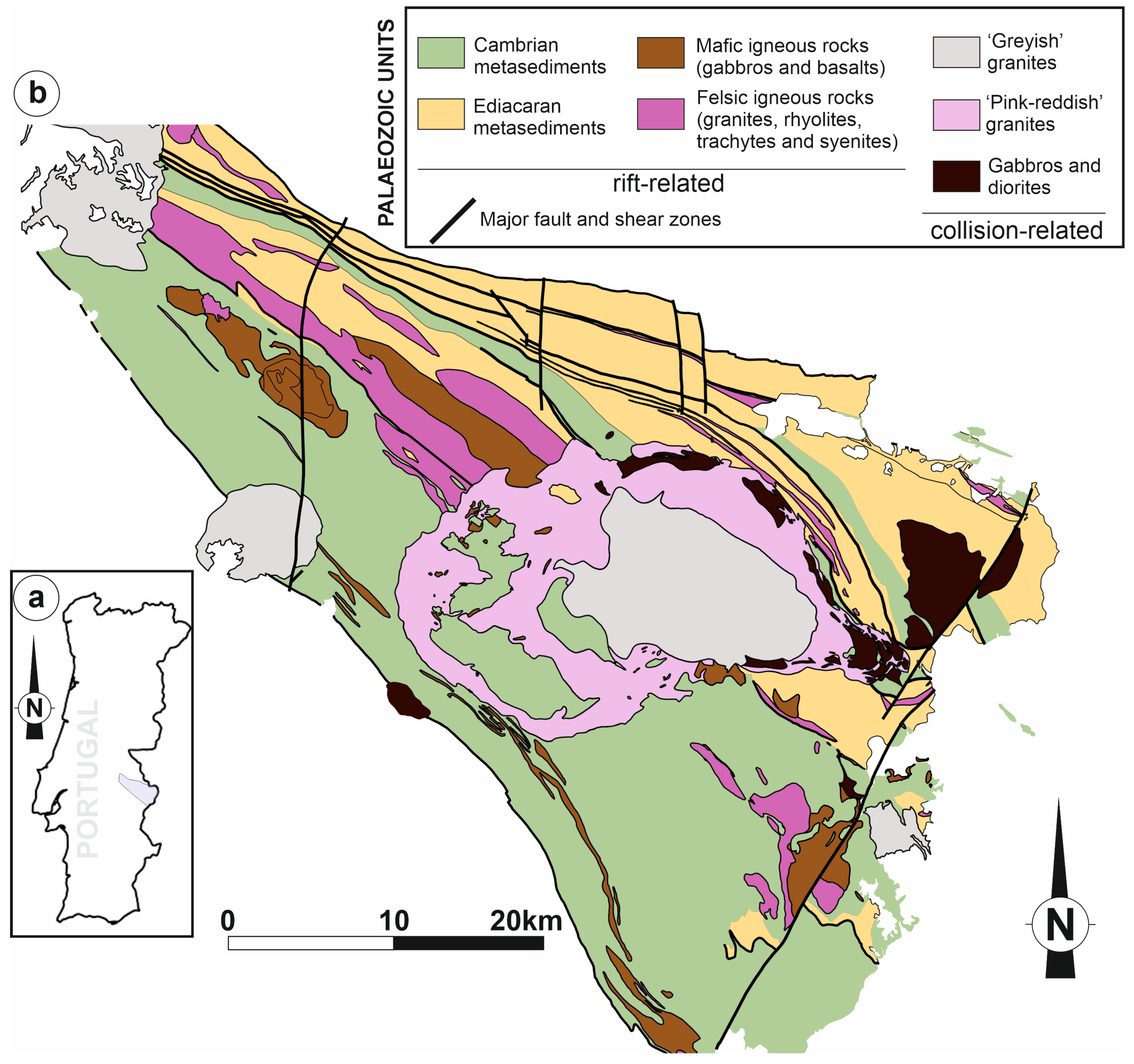
Figure 2. Geological map of the asymmetrical Santa Eulália Plutonic Complex (SEPC), with distinction of the different pinkish facies of the G0 group, as well as the different grey rocks from the G1 group (in some works the medium- and fine-grained grey facies are referred to as G2 and G3 facies respectively). The distinction of granite types based on textural aspects (grain size and colour) was made for ornamental purposes. Adapted from [2,24]. Besides the fracture lines, dashed contours indicate the country rocks enclaves (roof pendants), and the full lines indicate the contour of the three groups.

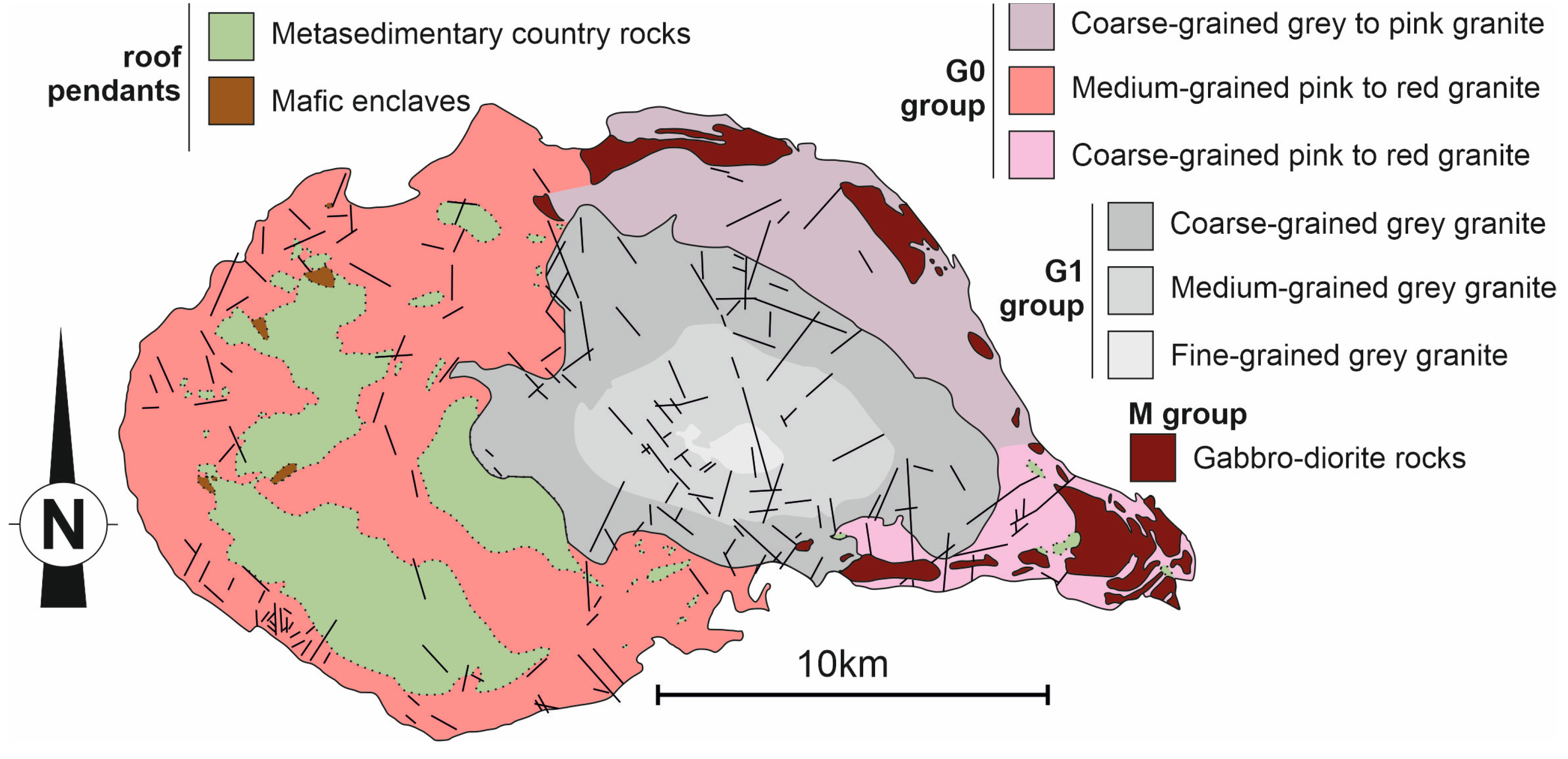
Figure 3. Field aspects of the inner rocks of the SEPC, that correspond to the G1 group rocks. (a) Looks of the medium-grained grey granite quarry (adjacent to Santa Eulália village). (b) Trails of micaceous schlieren indicative of upwards magmatic flow on the medium-grained grey granite (for some authors referred to as G2 facies). (c) General texture of the coarse-grained grey granite facies, on the external belt of the G1 group (d) Outcrop of typical joint fractures observed throughout the SEPC granites.

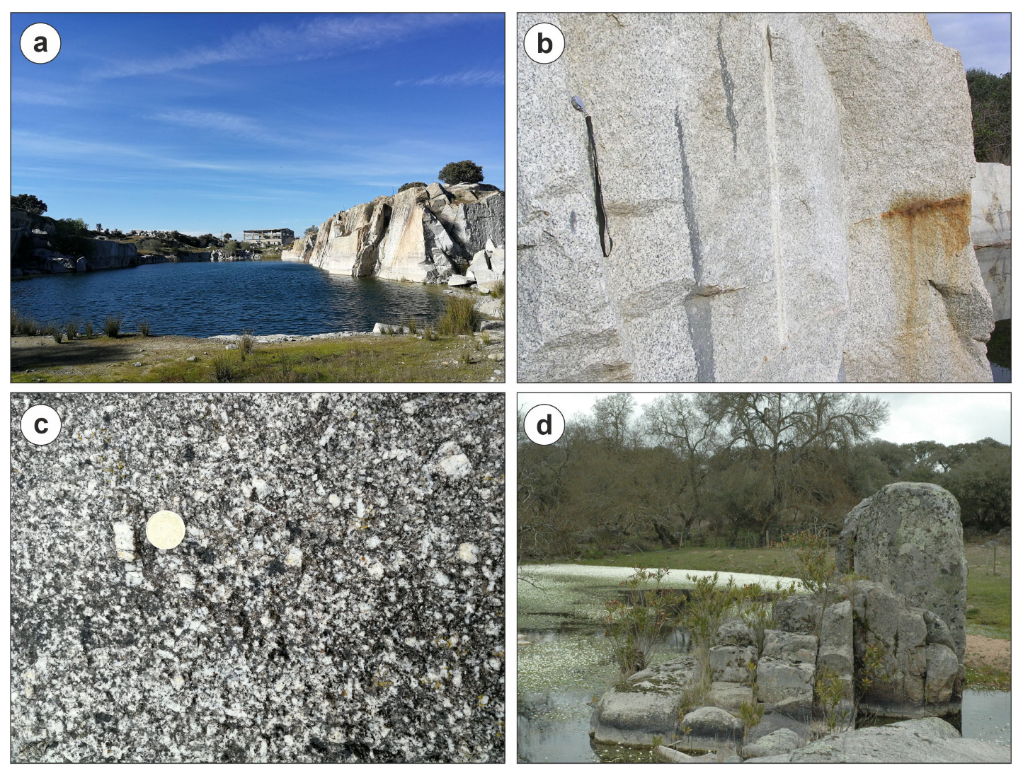
Figure 4. Field aspects of the G0 group rocks. (a) Landscape on a medium-grained reddish-pink granite quarry in the vicinity of the Monforte village (western facies of G0). (b) General texture of the coarse-grained reddish-pink granite facies from the southeastern part, hosting a composite enclave (xenolith). (c) General texture of the coarse-grained greyish-pink granite from the northwest region, with abundance of biotite. (d) Exposure of a country rock roof-pendant (impure marble with evidence of contact metamorphism) overlaying the medium-grained reddish granite (enclave from the western facies).

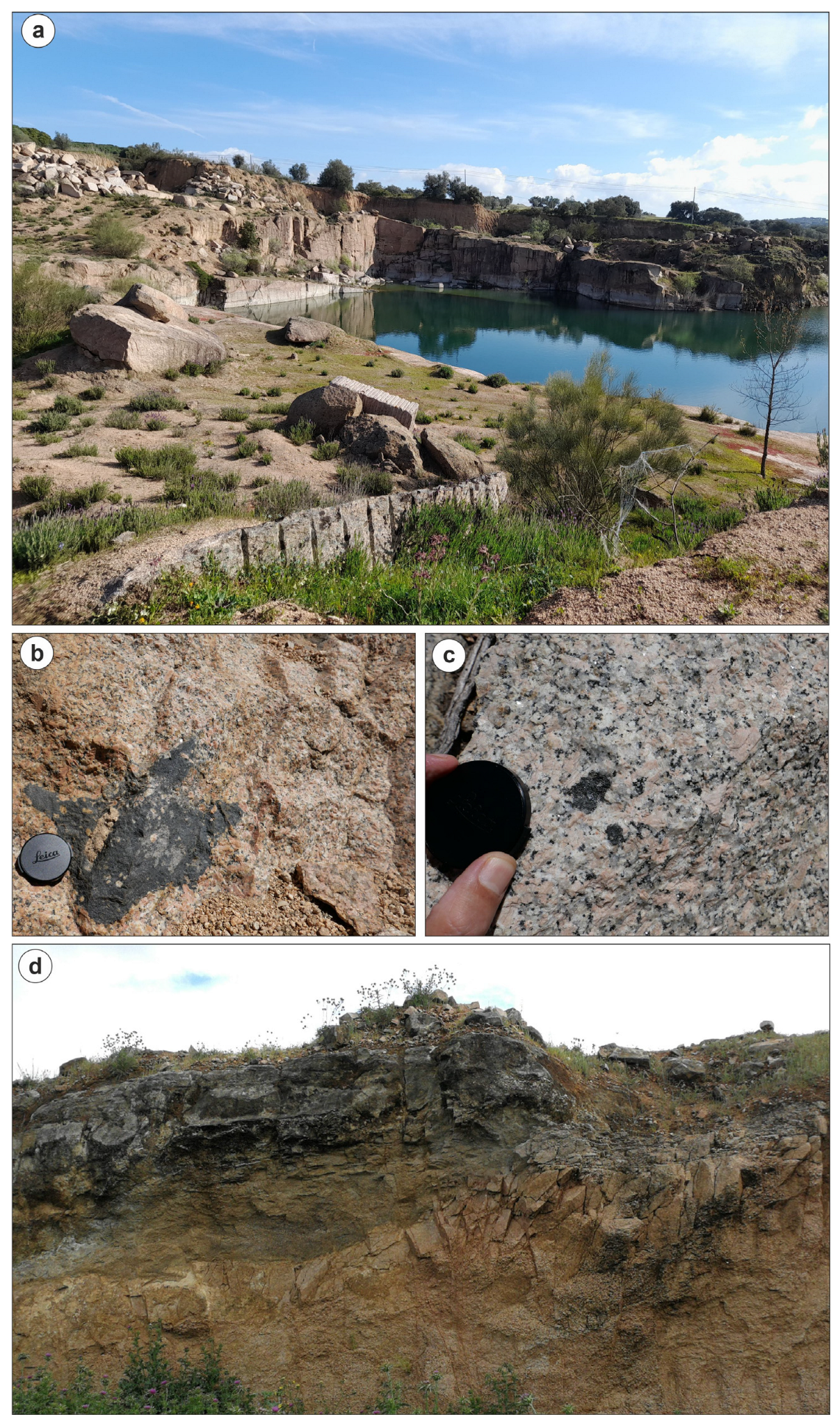
Figure 5. Field aspects of the M group rocks. (a) Sharp contact with the G0 group, in the easternmost part of the SEPC. (b) Common outcrops found in the region, showing the mingling and mixing/unmix textures of the gabbro-diorite rocks. (c) A mesoscale example of the dynamic crystallization zone for the rocks of the M group, with magma mingling under the form of irregular “fluid” boundaries of the diorite entrainment before the complete crystallization (up), and a diorite planar structure with internal flow, possibly indicating a compositional layering (down). (b) and (c) located in the northern region.

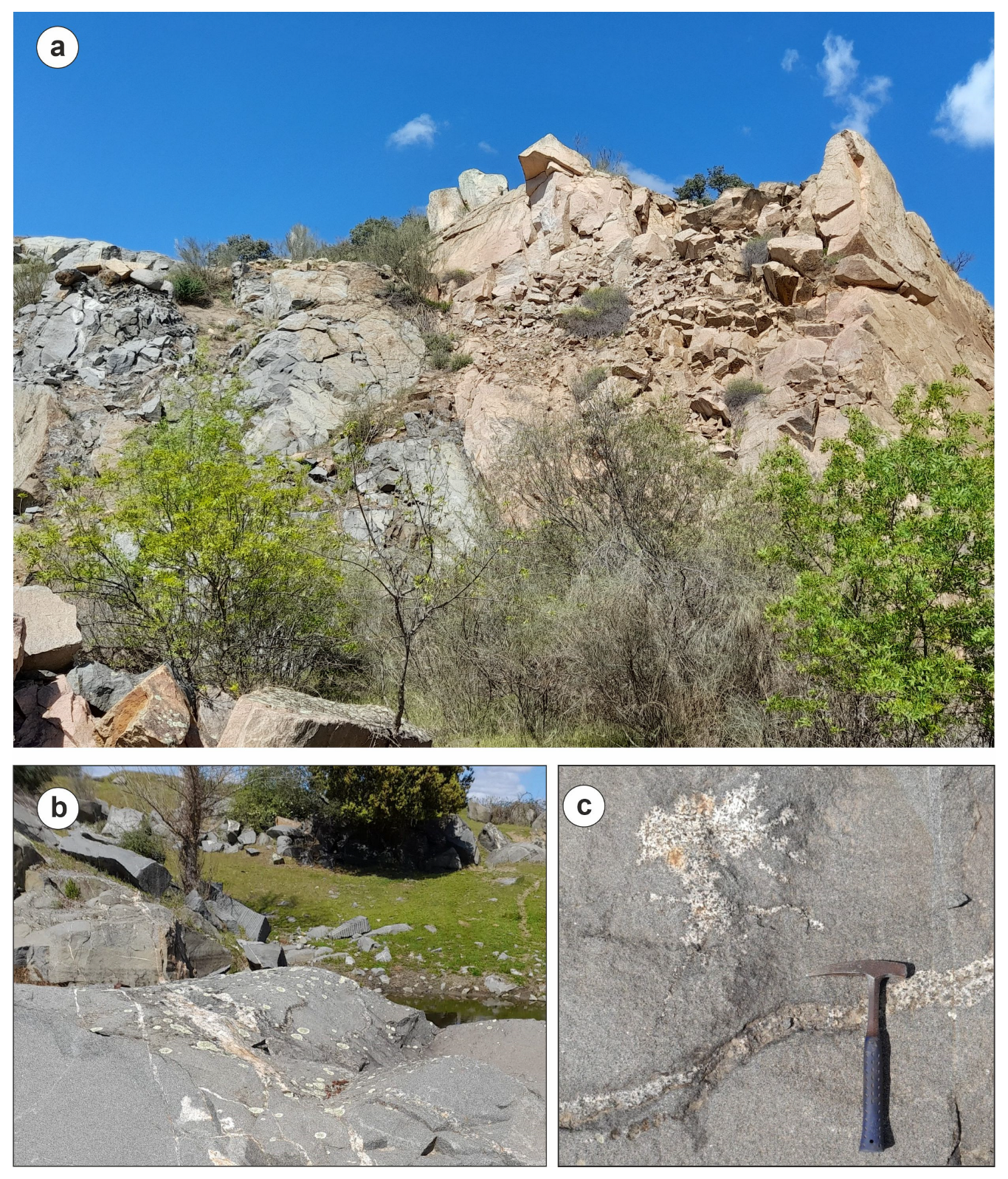
Figure 6. Workflow of the methods used in this study, with the steps from data acquisition to the final Random Forest-produced maps of predicted lithologies of the SEPC.

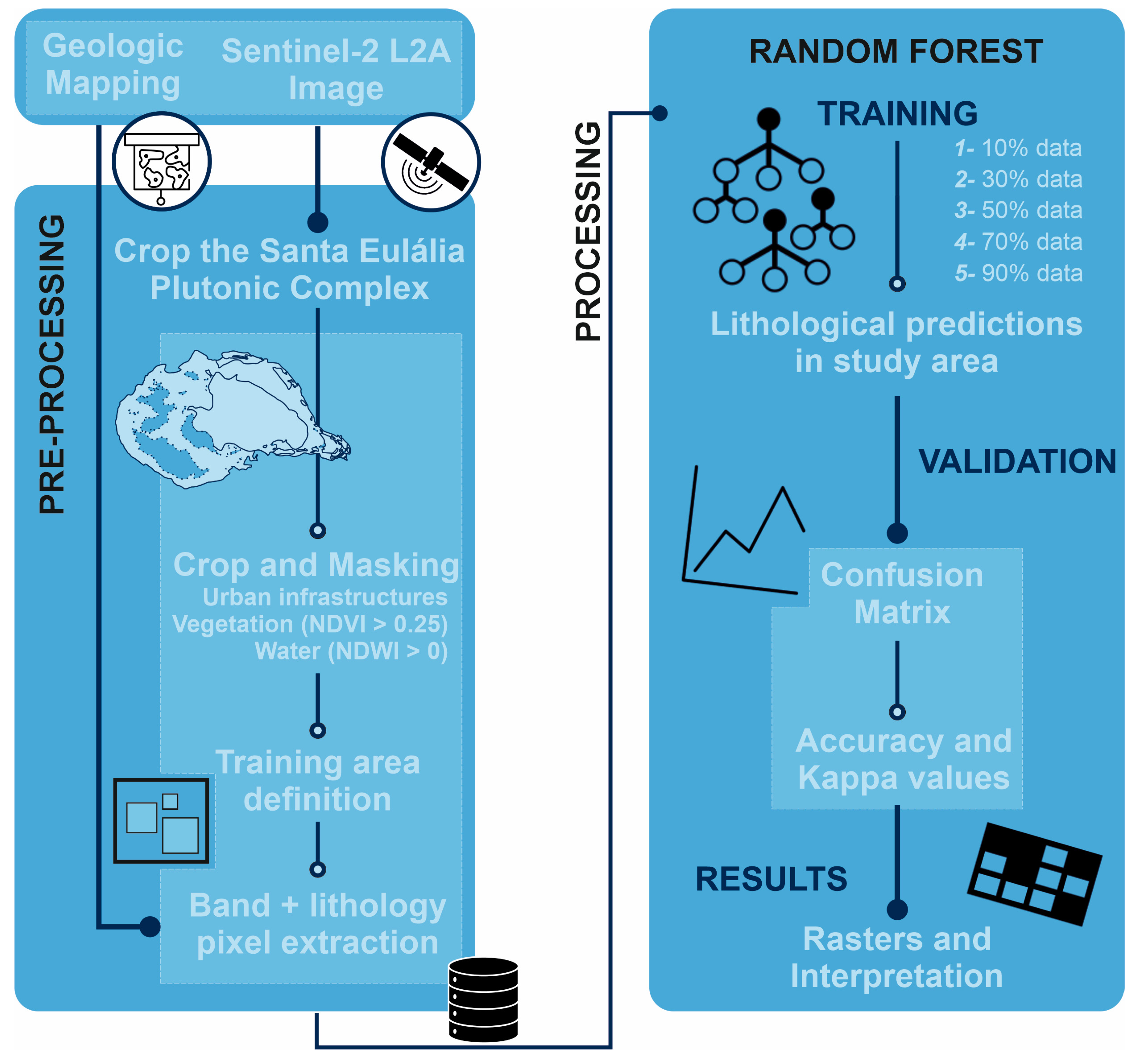
Figure 7. Sections of exposed rocks and soils for the SEPC groups chosen for Random Forest model training areas. Each section is numbered 1 to 39 (see supplementary materials).

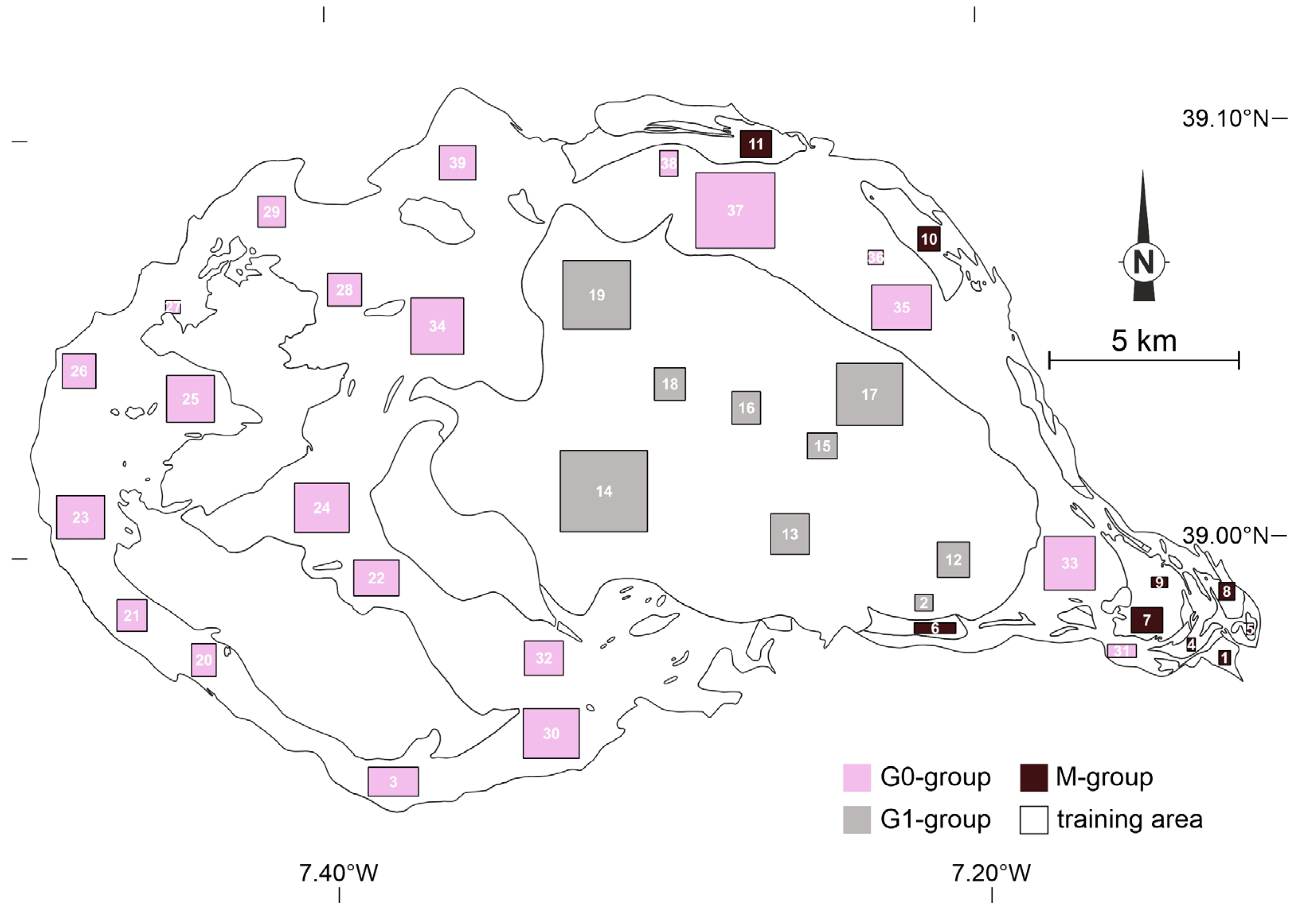
Figure 8. Atlas with representative examples of the SEPC groups. Original – original satellite image; Masked – satellite image after masking vegetation, water and urban infrastructures; CLC18 – Corine Land Cover 2018 classifications; NDVI – NDVI values (-1 to 1); SS – Spectral signatures. In CLC18: 131- Mineral extraction sites; 211- Non-irrigated arable land; 223- Olive groves; 231- Pastures; 244- Agro-forestry areas; 512- Water bodies.

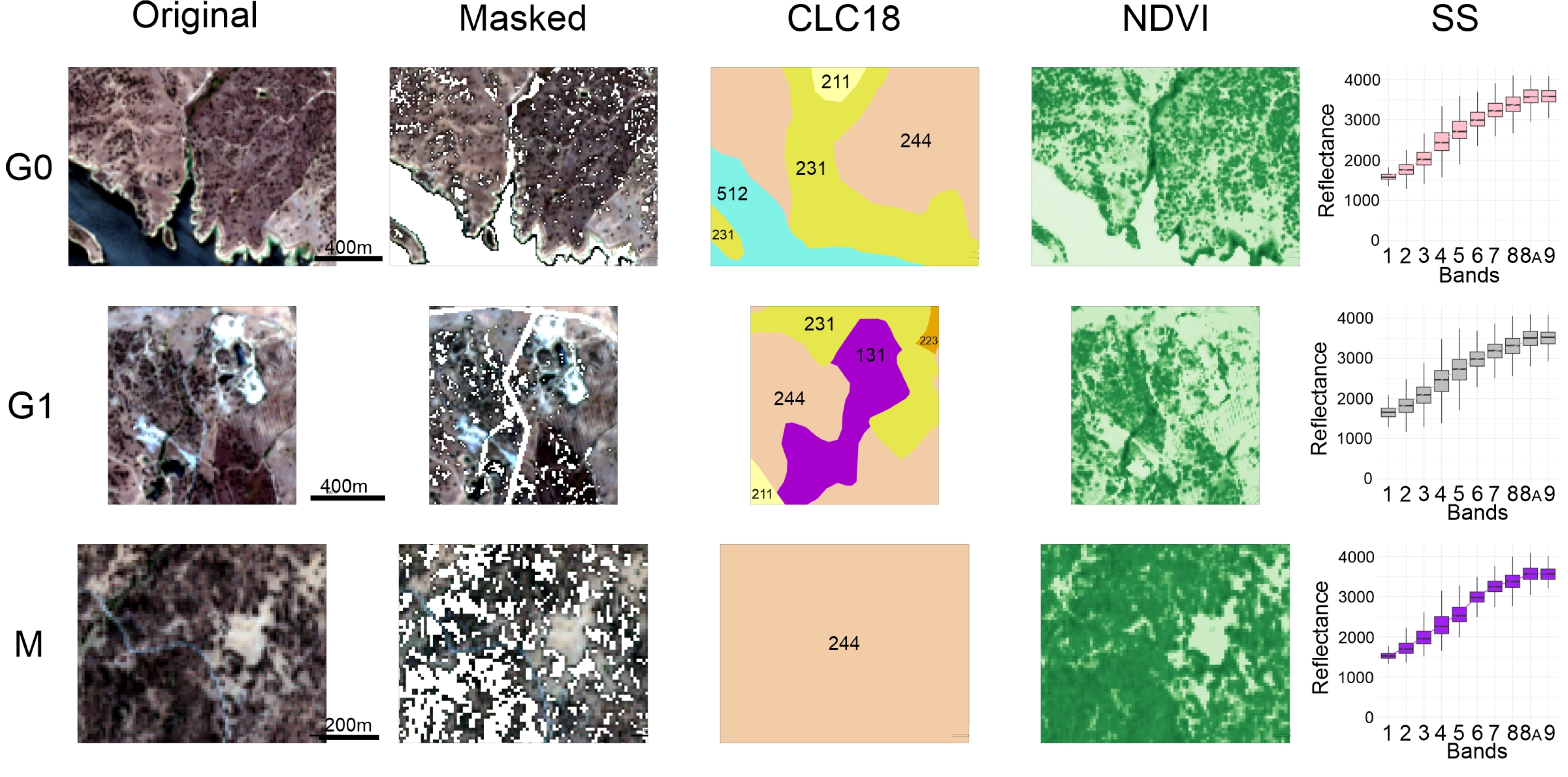
Figure 9. Correlation matrices. A – Original data; B – Complete dataset; C – Subset dataset.

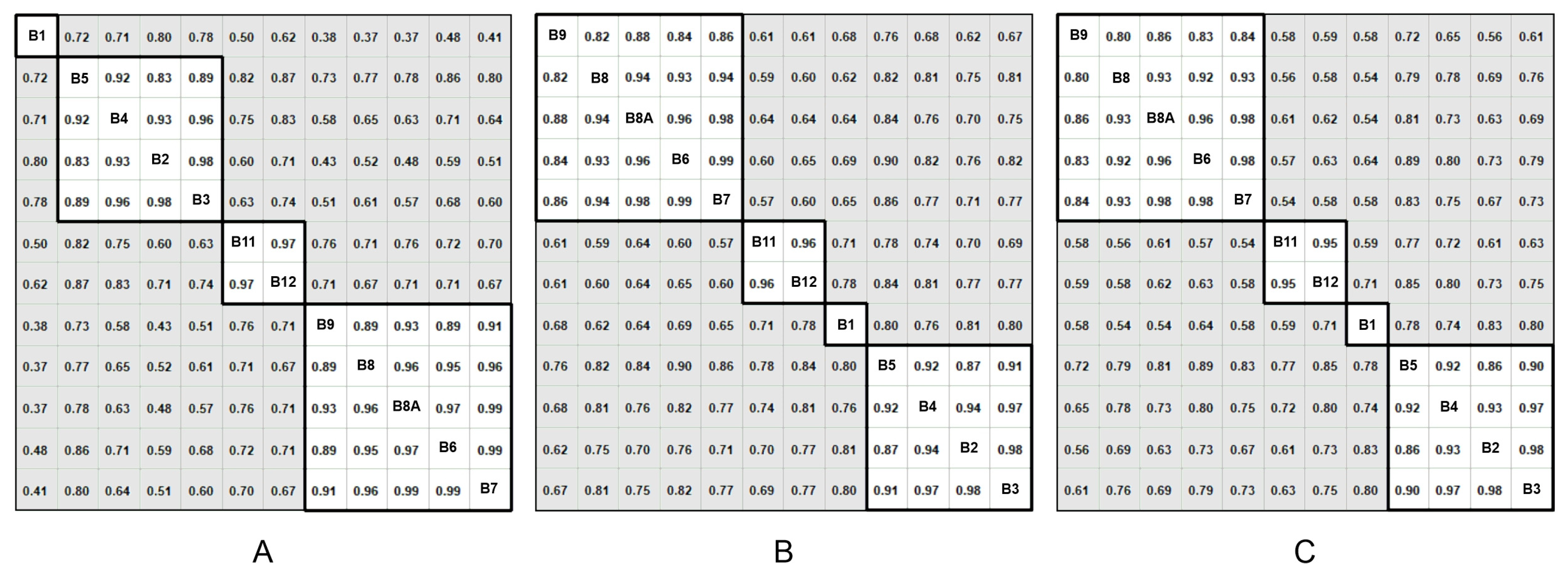
Figure 10. User (a) and Producer (b) accuracies for the SEPC groups using the Complete model for test dataset predictions. The dashed lines connecting the accuracies represent the slope variations between increasing model percentages. The horizontal lines mark values for suggested perfect, good, moderates, poor and very poor predictions.

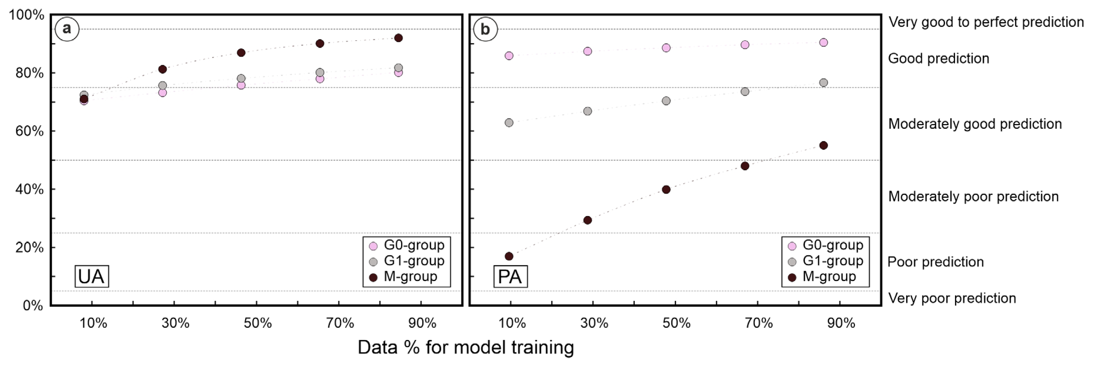
Figure 11. User (a) and Producer (b) accuracies for the SEPC groups using the Complete model for SEPC predictions. The dashed lines connecting the accuracies represent the slope variations between increasing model percentages. The horizontal lines mark values for suggested perfect, good, moderates, poor and very poor predictions.

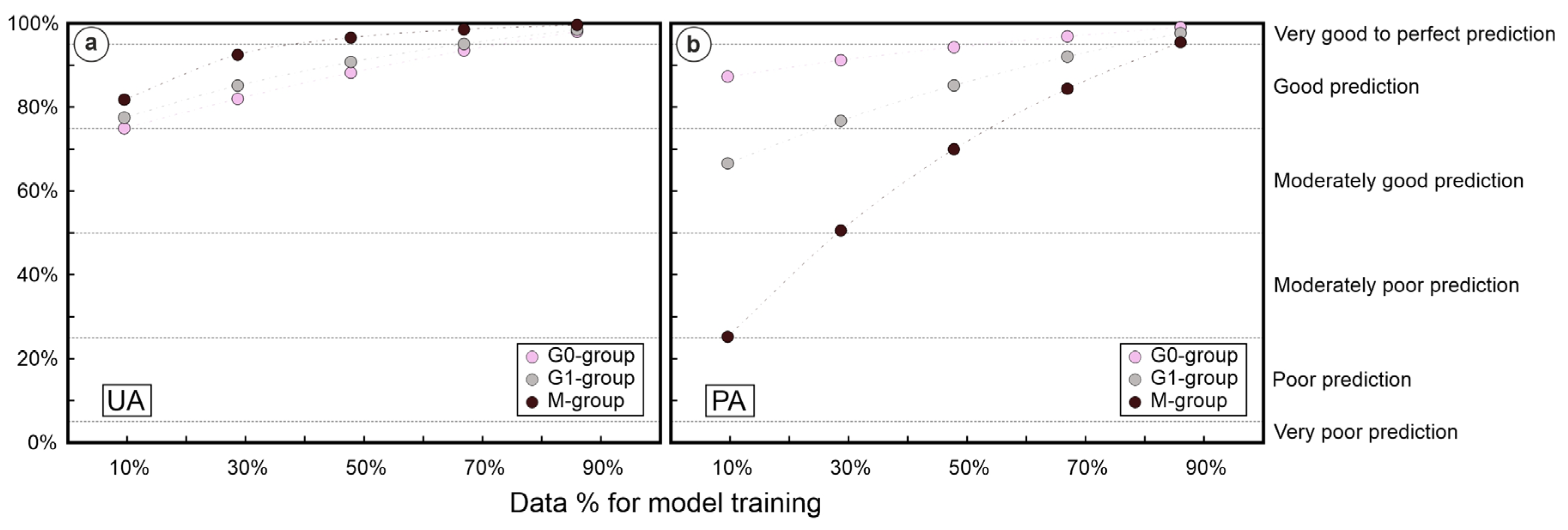
Figure 12. User (a) and Producer (b) accuracies for the SEPC groups using the Subset model for test dataset predictions. The dashed lines connecting the accuracies represent the slope variations between increasing model percentages. The horizontal lines mark values for suggested perfect, good, moderates, poor and very poor predictions.

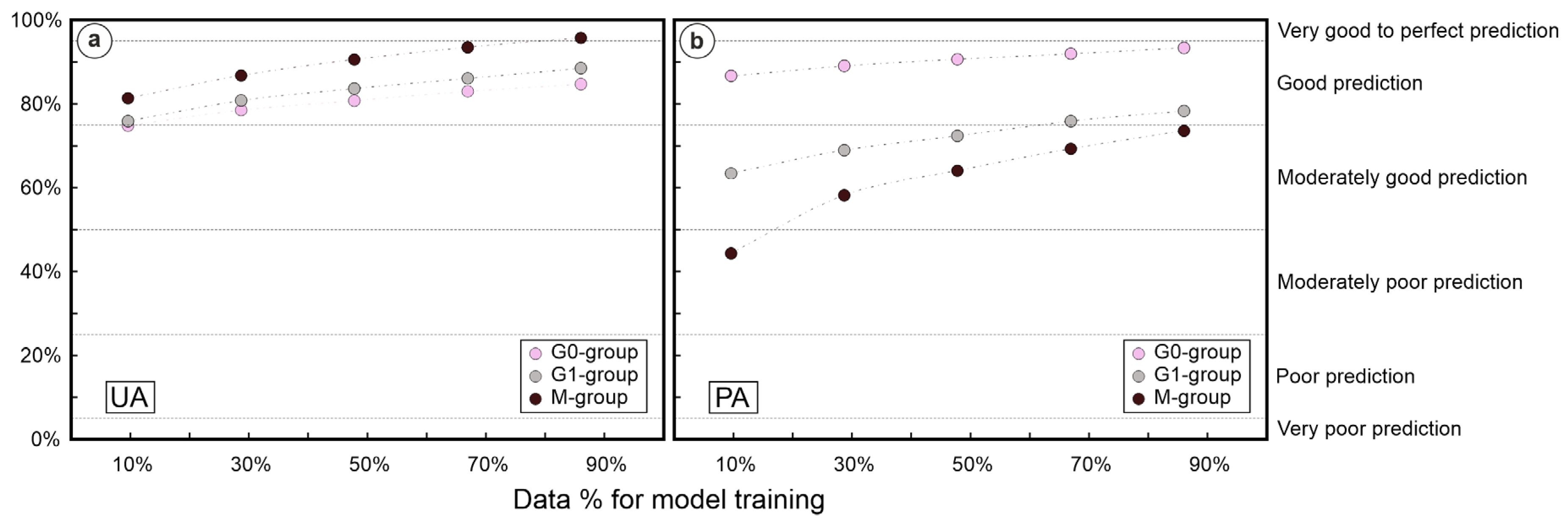
Figure 13. User (a) and Producer (b) accuracies for the SEPC groups using the Subset model for SEPC predictions. The dashed lines connecting the accuracies represent the slope variations between increasing model percentages. The horizontal lines mark values for suggested perfect, good, moderates, poor and very poor predictions.

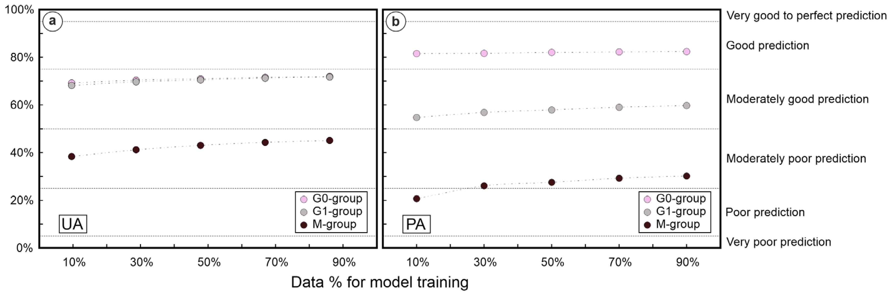
Figure 14. Map results for SEPC group predictions using (a) Subset 90% training sample size, and (b) Complete 10% training sample size. (c) Areas of mismatched predictions between the models, expressed by the blue pixels. Pink pixels refer to G0 group, grey pixels to G1 group rocks, and brown pixels to the M group.

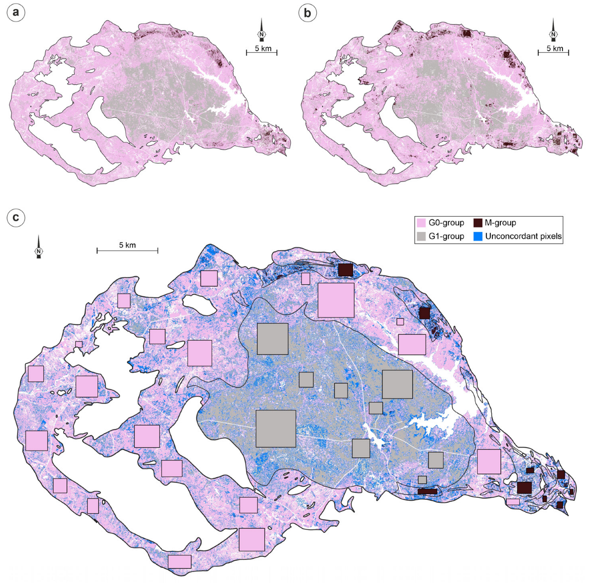
Table 1. List of main designations of the SEPC rocks exploited as dimension stones, for interior and exterior uses. Designations from [33].

Industrial designation¹	Group	Facies	Colour	Grain Size
Cinzala – Cinzento Santa Eulália	G1	G2 facies	Grey	Medium-fine
Cinzento Arronches	G1	G2 facies	Grey	Medium
Rosa Arronches	G0	Northeast	Greyish-pink	Coarse
Rosa Monforte	G0	Western	Strong reddish-pink	Medium
Rosa Santa Eulália	G0	Western	Reddish-pink	Medium-coarse
Vermelho de Barbacena	G0	Western	Strong reddish-pink	Medium
Favaco	M	Eastern²	Dark grey	Medium-fine
Gabrodiorito de Arronches	M	Northern²	Dark grey	Medium-fine

¹ Name given, with reference to local municipalities. ² Gabbro-diorites from the M group lenses in these regions of the SEPC.

Table 2. Pixel proportion and frequency of each lithological group for the three datasets.

Dataset	G0 group	G1 group	M group	Total
Original	58.32% 1887765	35.73% 1156534	5.95% 192743	3237042
Complete	56.53% 1574916	37.74% 1051477	5.73% 159657	2786050
Subset	55.94% 206644	38.40% 141839	5.66% 20888	369371

Table 3. Descriptive statistics (minimum, median, and maximum) of each band value for considered datasets.

Measure	Dataset	B1	B2	B3	B4	B5	B6	B7	B8	B8A	B9	B11	B12
	Original	1137	1014	978	1054	1012	957	940	758	972	1258	1185	1150
Min	Complete	1137	1014	978	1059	1031	1026	1010	1128	1062	1258	1297	1246
	Subset	1256	1025	1072	1077	1126	1049	1062	1128	1088	1419	1421	1312
	Original	1625	1759	2024	2430	2718	3020	3258	3396	3613	3625	5185	4065
Median	Complete	1634	1789	2064	2488	2767	3035	3266	3402	3625	3637	5291	4167
	Subset	1615	1766	2030	2440	2718	3006	3238	3374	3597	3613	5224	4089
	Original	4242	7908	8520	8576	8145	7703	7511	7788	7231	5323	7533	7414
Max	Complete	4218	6324	6016	6104	6929	6714	6556	6428	6297	5323	7313	6737
	Subset	3596	4804	5012	5256	5260	5111	5365	5764	5390	4854	6940	6622

Table 4. Validation metrics considered for Complete model performance on the 5 trained models on Random Forest used to predict the test dataset. Kappa coefficient strength of agreement designation from [41].

Training sample size	OA	Avg. UA	Avg. PA	Kappa Coeff.
10%	73.26	73.47	55.25	0.47 - moderate
30%	76.33	78.88	61.21	0.53 – moderate
50%	78.98	82.42	66.34	0.59 – moderate
70%	81.21	84.88	70.43	0.63 – substantial
90%	83.26	86.81	74.11	0.68 – substantial

Table 5. Validation metrics considered for Complete model performance on the 5 trained models on Random Forest used to predict the SEPC. Kappa coefficient strength of agreement designation from [41].

Training sample size	OA	Avg UA	Avg PA	Kappa Coeff
10%	75.94	78.12	59.72	0.52 – moderate
30%	83.43	86.58	72.85	0.68 – substantial
50%	89.49	91.88	83.17	0.80 – substantial
70%	94.36	95.74	91.13	0.89 – almost perfect
90%	98.33	98.75	97.41	0.97 – almost perfect

Table 6. Validation metrics considered for Subset model performance on the 5 trained models on Random Forest used to predict the test dataset. Kappa coefficient strength of agreement designation from [41].

Training sample size	OA	Avg UA	Avg PA	Kappa Coeff
10%	75.30	77.31	64.77	0.52 - moderate
30%	79.54	81.99	72.03	0.60 - moderate
50%	82.08	84.96	75.65	0.66 - substantial
70%	84.45	87.49	78.99	0.70 - substantial
90%	86.44	89.61	81.72	0.74 - substantial

Table 7. Validation metrics considered for Subset model performance on the 5 trained models on Random Forest used to predict the SEPC. Kappa coefficient strength of agreement designation from [41].

Training sample size	OA	Avg UA	Avg PA	Kappa Coeff
10%	67.95	58.59	52.33	0.37 – fair
30%	69.12	60.43	54.86	0.40 - fair
50%	69.81	61.52	55.84	0.41 - moderate
70%	70.45	62.39	56.85	0.42 - moderate
90%	70.84	62.91	57.44	0.43 - moderate

Disclaimer/Publisher’s Note: The statements, opinions and data contained in all publications are solely those of the individual author(s) and contributor(s) and not of MDPI and/or the editor(s). MDPI and/or the editor(s) disclaim responsibility for any injury to people or property resulting from any ideas, methods, instructions or products referred to in the content.

© 2024 by the authors. Licensee MDPI, Basel, Switzerland. This article is an open access article distributed under the terms and conditions of the Creative Commons Attribution (CC BY) license (http://creativecommons.org/licenses/by/4.0/).

Copyright: This open access article is published under a Creative Commons CC BY 4.0 license, which permit the free download, distribution, and reuse, provided that the author and preprint are cited in any reuse.

Downloads

Views

Comments

Subscription

Notify me about updates to this article or when a peer-reviewed version is published.

MDPI Initiatives

Important Links

Choose an area of interest and we will send you notifications of new preprints at your preferred frequency.

Disclaimer