
Submitted:
19 November 2024
Posted:
20 November 2024
You are already at the latest version
Abstract
How can we validate a given Multiple-Criteria Decision-Making (MCDM) approach and compare it to other MCDM methods? This question is not addressed in MCDM literature. This paper presents a novel out-of-sample approach using in-sample (e.g., 70%) data to assess the parameters of a given MCDM model and validate the model using out-of-sample (e.g., 30%) data. MCDM models are ranked based on their accuracies of predicting the out-of-sample data using several randomly selected replicas.
We develop a new class of MCDM models based on Geometric Dispersion Theory (GDT) that was recently developed for decision-making under risk. MCDM-GDT is based on a convex combination of maximizing an additive utility function (an arithmetic function) and a multiplicative utility function (a geometric function); this MCDM-GDT function is non-additive and non-linear in criteria and in weights of importance of criteria. A special case of MCDM-GDT is a highly effective concave utility function using k+1 parameters where k is the no. of criteria.
We apply MCDM approach for selection of the best wind farm location in Saudi Arabia using 30 expert decision makers (DMs). Then we provide a detailed comparison of several well-known MCDM methods and MCDM-GDT using the out-of-sample approach. The results indicate that most of MCDM methods, except MCDM-GDT, have poor predictive performances.
We also develop a new model for group decision-making using a new nonlinear aggregation of the ratings of DMs based on MCDM-GDT; we show that this model has advantages to using the commonly used weighted average rating of DMs.
Keywords:
MCDM
; out-of-sample validation
; geometric dispersion theory
; wind farm
; group decision-making
; multi-MOORA
; TOPSIS
; VIKOR
; generalized goal programming
1. Introduction
Despite all theoretical and methodological developments, the main question of how and why one should choose one multi-criteria decision-making (MCDM) model (method) over another has remained a puzzle. Ceballos et al. (2016) provides a comprehensive analysis of comparing the similarity of MCDM models based on simulated data. In this paper, for the first time, we suggest how to answer this puzzle by comparing several important MCDM models using real-world data. We show a novel approach based on using in-sample data (e.g., 70% of data) to assess the parameters of a given MCDM model and then validate the model using out-of-sample data (e.g., the remaining 30%). Validation of each model is based on the accuracy of predicting the 30% out-of-sample data which was not used to assess the parameters of the given model. Based on Malakooti (2018, 2024) and Malakooti et al., (2021), we propose using out-of-sample approach to compare the effectiveness of different MCDM methods for predicting DMs rating and ranking of alternatives.
Over the past six decades, MCDM techniques emerged with wide-ranging applications. Developments of MCDM methods were based on axiomatic and theoretical foundations, reasonable/appealing methodologies, aesthetics of methods, fuzzy set data, or easiness of assessment such as using direct ratings or interactive methods. Some notable MCDM methods include the elimination and choice translating reality (ELECTRE) method by Bernard Roy and his research team in the early 1970s, classical mut-attribute utility theory approach (e.g. see Keeney and Raiffa, 1993), and the analytical hierarchy process (AHP), introduced by Thomas Saaty in the 1980s (e.g., see Saaty, 2006, 2008). Additionally, methods like the simple additive weighting (SAW) technique, developed by Ching-Lai and Kwangsun Yoon (Kahraman et al., 2003), have found applications in various domains, including water management and financial decision-making. Also, a family of outranking methods such as PROMETHEE (Preference Ranking Organization Method for Enrichment Evaluations) has captured a lot of attention; see, Bezadian et al. (2010). Multicriteria optimization where objectives (criteria) are functions of decision variables adds an additional level of complexity for solving MCDM problems (see Ehrgott, 2005). Furthermore, interactive MCDM methods were developed by requiring minimum information from the decision maker (DM) to find the best (compromise) solution (see Ch. 2 of Malakooti, 2014 for a review of MCDM methods; also see Zavadskas et al., 2014).
In this paper, we also develop MCDM-GDT method based on Risk-GDT which was recently developed by (Malakooti 2018, 2024; Malakooti et al., 2021). MCDM models such as additive, multiplicative, concave, mixed concave & convex utility functions, minimizing distance to ideal points, and maximizing distance to nadir points can be presented as a special case of MCDM-GDT. Special cases of MCDM-GDT can have one parameter and up to (2k+2) parameters where k is the no. of criteria. We will show how to find the most parsimonious model (with the least no. of parameters) that has the best accuracy in out-of-sample experiments for a given application, to achieve this we experiment with a no. of models attempting to reduce their no. of parameters while maximizing the accuracy of prediction.
In this paper, we compare various well-known MCDM methods, including the additive multiple attribute utility functions, the Keeney multiple attribute multiplicative utility function, a variation of goal programming, the analytic hierarchy process (AHP), the quadratic regression model, variations of methods discussed in Ceballos et al. (2016), and variations of MCDM-GDT. We will show that a special case of MCDM-GDT, using k+1 parameters, out-ranks all other MCDM methods with any no. of parameters.
One significant application of MCDM is in the energy sector for the evaluation and optimization of wind farm locations. Research in this field has predominantly focused on the strategic placement or directionality of turbines within designated locations, as explored by Hou (2017), and the application of integer programming to optimize the placement of each turbine within a grid, thereby reducing the required number of wind turbines, a topic investigated by Manousakis et al. (2021). Additionally, other research delves into the broader spectrum of wind farm layout optimization (Wan et al., 2010; González, 2010). Several MCDM methods have been used to evaluate wind farm location selection, for example see Tsoutsos et al. (2009). Case studies, such as the one conducted for a wind farm project in China (Lee et al., 2008), have demonstrated the effectiveness of AHP in this context. Moreover, AHP and its fuzzy variants have been employed in farm allocation decisions in Malaysia (Hwang et al., 2011). Other MCDM methods, such as non-additive interactive and aggregative decision-making (NAIADE), have also been applied to assess wind energy plants (Cavallaro and Ciraolo, 2005). This paper presents a comprehensive study focused on identifying and ranking multiple criteria problems with application to wind farms location selection across 13 regions in Saudi Arabia, a country with significant potential for renewable energy development. Our study utilizes data on three criteria: average wind power density, average wind speed, and terrain suitability for the thirteen regions in Saudi Arabia, obtained from the Saudi Arabian National Center for Meteorology.
We apply all MCDM models considered in this paper to this problem of wind farm location selection in Saudi Arabia using thirty expert DMs. We show how to find the most accurate MCDM model and apply it to this location problem using ratings of a group of DMs.
We develop two methods for addressing the integration of group DMs (experts) ratings of different MCDM alternatives: first by using average ratings of all experts, and second by using an extension of MCDM-GDT that allows for aggregation of experts’ assessment such that the effects of extreme opinionated experts are minimized while their opinions are not eliminated.
To the best of our knowledge, the geometric dispersion theory (GDT) models have been utilized only for risk analysis (Malakooti, 2018, 2024; Malakooti et al., 2021; Komaki et al., 2019). This study marks the inaugural application of GDT models to address MCDM problems and its application to wind farm locations in Saudi Arabia.
The remainder of this paper is structured as follows: Section 2 provides an overview of classical MCDM methods that will be used in this study. Section 3 presents the new MCDM-GDT method and its special cases that can be easily assessed. Section 4 layouts the materials and data of the application to be used in experiments. Section 4 also provides the description of wind farm selection in Saudi Arabia as an application. Section 5 shows the experiments approach. Section 6 illustrates results of using 100% of data to predict 100% of data. Section 7 presents result of using 70% of data to predict the remaining 30% of data. Section 8 discusses the alternative approach for solving the group decision making problem. Section 8 also discusses how to aggregate ratings from multiple decision-makers using the newly developed MCDM-GDT. Section 9 is the conclusion. Additionally, we offer a web supplement2 (Altowijri, Malakooti and Wang, 2024) containing datasets, code, programs, notations, and extensions for this research. Abbreviations are presented at the end of the paper.
2. Review of Applicable MCDM Methods for Comparative Analysis
2.1. Notations of the MCDM Problem
Given a set of alternatives, MCDM is concerned with identifying the best (optimal or most compromise) alternative or ranking the set of alternatives for a given DM. In this paper, we assume the set of alternatives is discrete and there are no interactions among alternatives. We also assume that alternatives are associated with k no. of discrete criteria (also called objectives or attributes). All criteria are maximized. We will show how to assess the utility function and rank all alternatives.
Suppose that the set of alternatives is presented by S which contains n discrete alternatives where S = [, , …, ], or for j = 1, 2, …, n,. Each alternative is a k-tuple vector of criteria represented by = [] where for i = 1, 2, …, k. Assume all criteria are maximized. The well-known definition of efficiency is as follows.
An alternative is efficient (non-dominated) if there does not exist an alternative such that with at least one strict > for i = 1, 2, …, k.
The definition of efficiency (or non-dominancy) can be used to identify inefficient (inferior or dominated) alternatives. If the purpose is to find the best MCDM alternative, inefficient alternatives can be discarded (e.g., see Keeney and Raiffa, 1993, and Malakooti, 2014).
To simplify solving the MCDM problem, a common practice is to normalize the values of each criterion from 0 to 1, where 0 is the worst and 1 is the best value. Each criterion can be normalized as follows:
First, we find the range of each criterion (objective), for i = 1, 2, …, k.
To utilize multiplicative forms (and avoid extreme values of avoid 0 and 1), without loss of generality, we normalize each criterion and present them by fi, for i = 1, 2, …, k, such that 0 < fi, < 1 for all i. To find normalized values, we can use any random constant δ such that for all i. Experimentally, we found that MCDM models are not sensitive to the value of δ, thus we adopt a default value of δ = 0.01. Therefore, for any given alternative j, we use:
The result is 0.01 ≤ fi,j ≤ 0.99 for all i. Therefore, we define Fj as the vector of the normalized values of for j = 1, 2, …, n.
2.2. Linear Value Utility Function (LV) without Using Criteria Value Functions
Historically, the additive utility functions have been used to rate and/or rank multi-criteria alternatives; for a review see Jacquet-Lagreze et al., (1982) and Keeney and Raiffa, (1993). The simplest form of additive utility function is Linear Value utility (LV) as shown in Eq. (2.2) where each fi is maximized.
where w1 > 0, w2 > 0, …, wk > 0 and w1 + w2 + … + wk = 1.
LV = w1 f1 + w2 f2 + … + wk fk (Linear Value utility (LV))
Where wi is the weight of importance of criterion i, for i = 1, 2, …, k. These weights (parameters of LV) are solicited from the DM to reflect the importance of each criterion. All weights are positive numbers, and the utility function is maximized.
LV is a convex combination of all fi and wi >0, for all i, assures that LV is increasing in all fi. LV is simple to implement because it has only k parameters and has no interactions or dependencies among criteria (e.g., see Keeney and Raiffa, 1993 and Jacquet-Lagreze et al, 1982). Here, we emphasize that there could be many different forms of Utility functions, U, but the efficiency principle of MCDM requires U to be increasing in all fi.
2.3. Additive Utility Function with k Criteria Value Functions (LV-kV)
Additive Utility Function with k Criteria Value Functions (LV-kV), known as additive MAUF, is the generalized form of LV function by incorporating value functions of criteria, (e.g., see Keeney and Raiffa, 1993). The utility function, U, is the weighted sum of value functions of criteria as shown below.
where w1 > 0, w2 > 0, …, wk > 0, and w1 + w2 + … + wk = 1.
U = w1v1(f1) + w2v2(f2) + … + wkvk (fk) (General LV-kV)
The value function vi(fi) is an increasing function of fi. U is an increasing function of vi(fi) for all i ; this is enforced by w1 > 0, w2 > 0, …, wk > 0 While LV is linear, LV-kV is nonlinear because each vi(fi) can be nonlinear. The convex or concave types of the value functions can capture different preferences and attitudes of decision-makers (e.g. see, Eintalu, 2019). Each value function can also be S- or inverted S-shaped or may have more complex shapes (e.g., see Malakooti, 2015). Determining the shapes of value functions can be challenging and subjective, as it may requires experts’ inputs and/or data analysis. To simplify the process of assessment of value functions, in this paper, we use a one parameter power function to present the value function of each criterion as concave, convex, or linear as shown in Eq. (2.4).
The value function, vi(fi) is concave when αi < 1, convex when αi > 1, and linear when αi = 1.
Now using these functions in Eq. (2.3), we have Eq. (2.5). This function has 2k parameters.
where w1 > 0, w2 > 0, …, wk > 0 and w1 + w2 + … + wk = 1, αi > 0 for all i
2.4. Additive Utility Function with One Value Function for All Criteria (LV-1V)
To reduce the no. of parameters for LVG-kV (Eq. 2.5) model, we can use the same value function for all criteria, where for all i in Eq. (2.4). Such that The justification of using one value function for all criteria is given in Malakooti (2015). In this paper, we will test its validity using out-of-sample experiments. For LVG-1V, we have
where w1 > 0, w2 > 0, …, wk > 0 and w1 + w2 + … + wk = 1, and α > 0
Note that the composite utility function U in Eq. (2.6) is concave when α < 1, convex when α > 1.
2.5. A Summary of MCDM Models for Comparative Analysis
A summary of well-known important MCDM models is presented in Table 1 and details of these methods are explained in Appendices. We have also experimented with several other MCDM methods, including Zeleny’s (1982) aspirational methods for Euclidean norm and different versions of goal programming; however, in our sample vs. out-of-sample experiments, these methods performed poorly in predicting DMs’ behavior in rating multi-criteria alternatives. Therefore, here we only present MCDM methods that are most powerful in out-of-sample predictions.
Here we discuss how MCDM methods presented in Table 1 are related to MCDM models used in Ceballos et al. (2016). In this paper we use a simple linear normalization approach as presented in Eq. (2.1) while Ceballos et al. (2016) uses several different normalization approaches. Second, we consider a few simplified versions additive multiple attribute utility functions (MAUF) Eq. (2.3) (Keeney and Raiffa, 1993). MU-kV is a special case of multiplicative MAUF (Keeney, 1974). AHP-LV is related to ratio approach (Brauers and Zavadskas, 2010) which is one of the multi-MOORA (Multi-Objective Optimization on the basis of a Ratio Analysis) approaches. MAD-GP is related to the distance to ideal point and goal programming (Zeleny 1982, Tamiz et al. 1998) which are both related to TOPSIS (Technique for Order of Preference by Similarity to Ideal Solution) and VIKOR (VIse Kriterijumska Optimizacija kompromisno Resenje, in Serbian, Multiple Criteria Optimization Compromise Solution). Z-MAD-GP is a hybrid of distance to ideal point and LV (which is inspired by GDT approach of the next section based on (Malakooti 2014). QU is generalized LV based on quadratic nonlinear regression. In our experiments, we also used equal weights as it was done in Ceballos et al. (2016).
3. Multiple Criteria Decision Making-Geometric Dispersion Theory Method
The basic idea of GDT is that it is a hybrid function of arithmetic and geometric models which is truly nonlinear (neither arithmetic (e.g. additive) nor geometric (e.g. multiplicative) because while a geometric function can be transferred to an arithmetic function by a logarithmic transformation (i.e. it becomes an additive function), the GDT hybrid function cannot be transformed to an arithmetic (or additive) function.
The MCDM-GDT model is based on Risk-GDT developed by Malakooti (2018, 2024) and Malakooti et al. (2021). Here, we use the notations of Risk-GDT as applied to MCDM-GDT. MCDM-GDT complies with efficiency (non-dominancy) principle as can be derived from Malakooti (2018, 2024) proofs.
3.1. Concave Basic GDT-1 Model (without Value Functions)
GDT-1 is a nonlinear utility function that generalizes the linear additive utility function (Eq. 2.2). GDT-1 is a convex combination of additive and multiplicative functions as explained below. It has k + 1 parameters where k is the no. of criteria. See Table 2 for an overview.
Geometric value (GV) function is expressed as:
Note that GV is less than or equal to LV (Eq. 2.2). Geometric Deviation (GD) denotes the deviation of LV and GV. As the deviation among criteria decreases GV approaches LV and GD approaches zero.
GD approaches 0 as deviation among criteria diminishes. Specifically, GD=0 for all alternatives that have equal criterion values, i.e., for fi=fi+1 for i=1,2, …k-1. GDT–1 generalizes the well-known arithmetic mean and geometric mean functions (Malakooti, 2014, pp. 93-100). In general, U(LV, GD) has a nonlinear relationship between LV and GD where LV is maximized and GD is minimized. A special case of U(LV, GD) is linear relationship of LV and GD which results in GDT-1. GDT-1 is convex combination of LV and GV in which both LV and GV are maximized.
where -1<z≤0 is a coefficient to be assess by the DM. When z = 0, the utility function is additive (linear). Malakooti (2014, pp. 93-100) originally developed GDT-1 and named it Multiplicative-ZUT. He provided a direct assessment of the parameters of Eq. (3.3), in this paper we develop the indirect assessment of GDT-1 using ratings of DMs.
U = LV + zGD = (1 + z)LV – zGV (Concave GDT-1)
Using results from Malakooti (2018, 2024) and Malakooti et al. (2021), we can show that this function complies with the efficiency (non-dominancy) definition of MCDM. Furthermore, Malakooti (2018, 2024) shows that GDT-1, Eq. (3.3), is a concave function of fi for all i. Therefore GDT-1 is a concave function, which is assumed to be a desirable pattern in decision making.
GDT-1 offers a flexible framework for modeling utility functions that can capture both linear and nonlinear aspects of decision-makers’ preferences by assessing only k+1 parameters. It allows for the incorporation of the coefficient z, which enables adjustments between additive and multiplicative functions, making it adaptable to various decision scenarios.
GDT-1 can be interpreted as a hybrid of model of LV and GD (or XD). From MCDN point of view, this is a new generation of MCDM models with two level hierarchy, in the first level, LV and GV are maximized, while in the second level fi for all i are maximized. Therefore, GDT-1 can be considered as the combination of two different utility functions. We can interpret GDT-1 as a hybrid of model of LV and GD (or XD). From MCDM point of view, this is a new generation of MCDM models with two level hierarchy, in the first level, LV and GV are maximized, while in the second level fi for all i are maximized. Therefore, GDT-1 can be considered as the combination of two different utility functions.
We can simplify GDT-1 as a convex combination of LV and GV; here we must assess k weights and z, total of k+1 parameters. Keeney (1974, 1973) also provided a use of multiplicative functions; however, his utility function can be converted to an additive function by a logarithmic transformation. However, GDT-1 cannot be transferred to an additive function and has substantial nonlinearity in weights of importance wi for all i. This nonlinearity of GDT-1 provides the flexibility to solve real-world problems, as shown in this paper and in Malakooti (2018, 2024), Malakooti et al. (2021), Komaki and Malakooti (2019).
3.2. Basic GDT-2 Model (Without Value Functions)
Now, we define X-geometric value (XV) in Eq. (3.4). XV is greater than or equal to LV, therefore LV is the lower bound of LV. As deviation among criteria decreases, XV approaches LV. Now, we can define the X-geometric deviation (XD), (Eq. 3.4) to measure the deviation of XV from LV
XD approaches 0 as deviation among criteria diminishes.
In terms of properties, XV and XD are convex functions of all fi, and U = LV + zXXD is convex in all fi. Using LV and XD, we can define Convex GDT-1 as follows.
U = LV + zXXD = (1 – zX)LV + zXXV (Convex GDT-1)
Here we have k+2 parameters: k weights, z, and zX.
where -1 < z ≤ 0, 0 ≤ zX < 1, zX – z ≤ 1.
U = LV + zGD + zXXD = (1 + z – zX)LV – zGV + zXXV (Basic GDT-2)
When z = zX = 0, GDT-2 reduces to LV. The nonlinearity of GDT-2 provides substantial flexibility to solve real-world problems (Komaki and Malakooti, 2019). As shown in Malakooti (2018, 2024), Malakooti et al. (2021), in Eq. (3.6), (1 + z – zX)LV is linear, (– zGV) is concave, and (+ zXXV) is convex, therefore, this function is mixed concave and convex.
Because GDT-1 is concave, then Basic-GDT-2 is a mixed concave and convex function in fi. The GDT-2 model considers dispersion in criteria, which can be relevant in scenarios where criteria exhibit variations or uncertainty. It provides flexibility through the introduction of dispersion parameters, allowing decision-makers to control the level of dispersion in the utility function. GDT-2 offers a balance between linear and nonlinear components, making it adaptable to various decision-making contexts.
3.3. GDT-1 with k Different Value Functions
We can generalize GDT-1 by using value functions of criteria, vi(fi ) instead of fi for all i. LVG-kV is GDT-1 with k value functions is a nonlinear utility function having 2k + 1 parameter where k is the no. of criteria. The composite utility of all GDT models is calculated by Eq. (3.3). Here we generalize the Basic GDT model presented in Table 2.
For GDT-1 using concave value functions with each criterion (i.e. k value functions) (GDT-1-kV), we use LVG-kV (Eq. 2.5) and the geometric value (GVG-kV) function is given by combining Eq. (2.4) and (3.1):
GDG-kV can be derived from combining Eq. (2.4) and (3.2):
GDT-1-kV allows for the incorporation of individual value functions for each criterion, providing flexibility in modeling preferences that can capture concave and convex relationships between criteria through the value function. This makes it suitable for scenarios where criteria exhibit nonlinearity. The introduction of a multiplicative value function enables the representation of complex interactions among criteria. On the other hand, determining appropriate value functions and their parameters can be challenging and may require domain expertise.
When applying GDT-1 with one value function (GDT-1-1V) where , then we use LVG-1V (Eq. 2.6) and the geometric value (GVG-1V) and geometric deviation (GDG-1V) functions are presented below:
3.4. GDT-2 with k Different Value Functions
GDT for concave and convex utility with k value functions is a nonlinear utility function having 2k + 2 parameters where k is the no. of criteria. GDT-2 using k value functions (GDT-2-kV) can be derived from Eq. (3.4). The LVG-kV function and the geometric value (GVG-kV) function is already shown in Eq. (3.8) and (3.7). See Table 3 for an overview.
We define X-geometric value (XVG-kV) and X-geometric deviation (XDG-kV) as follows:
Now we can develop a special case of this GDT-2-kV using one common value function for all criteria (GDT-2-1V), we set , where the value function follows the same form as Eq. (2.4).
The X-geometric value with one value function (XVG-1V) is:
Thus, the X-geometric deviation with one value function (XDG-1V) can be derived:
GDT-2 (Eq. 3.15) combines the utility modeling capabilities of GDT with the introduction of a value function, allowing for a more comprehensive assessment of criteria. The model can handle both concave and convex utility functions, providing flexibility in addressing different decision-making scenarios. It offers a balanced approach between linear and nonlinear components, making it suitable for various applications (Malakooti, 2024).
U = LVG + zGDG + zXXDG = (1 + z – zX)LVG – zGVG + zXXVG
However, determining suitable values for z, zX, and α poses a challenge and may necessitate sensitivity analysis. Introducing additional parameters and a value function heightens the model’s complexity, demanding both data and computation resources. The precision of GDT-2-kV results hinges on the accurate specification of dispersion parameters, value functions, and weights.
3.5. Theoretical Foundation of MCDM-GDT: Satisfying Non-Dominancy (Efficiency), Concavity, and Mixed Concavity/Convexity
Here we discuss how to apply the theoretical results of Risk-GDT model of Malakooti (2018, 2024) and Malakooti et al. (2021) to MCDM -GDT of this paper. We propose that theories of Risk-GDT are applicable to MCDM-GDT by simply using wi of an MCDM problem instead of pi (which are probabilities in risk) and using fi (of an MCDM problem) instead of yi (which are consequences in risk). Then the proof of all theories can be found in Malakooti (2018, 2024) and Malakooti et al. (2021). These studies show that for risk problems all GDT problems generate first-order stochastic non-dominance solutions; and here for MCDM problems, MCDM-GDT models of this paper generate non-dominated (efficient) solutions. Also, GDT-1 is a concave function and GDT-2 is mixed concave and convex function.
Now consider value functions, if all v(fi) are concave (e.g. all αi < 1 in Eq. 2.4), GDT-1-kV is concave. Similarly using same value function for all criteria (e.g. α < 1 in Eq. 2.4), GDT-1-kV is also concave; this is the simplest form of a general concave GDT using k+2 parameters.
On the other hand, when v(fi) are concave or convex, GDT-1-1V and GDT-1-kV are mixed concave/convex function. We will discuss that these types of mixed concave/concave GDT have significant importance in explaining the MCDM problem application of this paper.
3.6. A Flowchart of Instruction: How to Assess and Use MCDM-GDT Models
In this section we discuss the approach for finding the special case of MCDM-GDT model which has the minimum no. of parameters to solve a given MCDM problem3. Consider MCDM models presented in Table 4 that shows special cases of General-GDT model (Eq. 3.15) in its first column. Our motto is to use the least no of parameters, therefore start by using default values of equal weights, and linear value functions, v(f)=f, i.e. α=1. In Table 4, Roman numerals are used to show the complexity of models in terms of increasing the no. of parameters. The simplest model is I, which uses one parameter, z, where equal weights and linear value functions are assumed, and the most complex model is XII which uses (2k+2) parameters where k weights (w1, w2, … wK) and k value functions using (α1, α2, … αK), z, and zX are used.
To solve an MCDM problem, start by dividing the data into two groups of in-sample (e.g. 70% of data) and out-of-sample (e.g. 30% of data), assess the parameters using in-sample data and test the validity using out-of-sample data. Start with the simplest model with the least no of parameters (e.g. model I), if the validation result (in out-of-sample) is not acceptable, then consider the next model with one more parameter, repeat adding one more parameter until the validation process is satisfactory. This way, the model with the minimum no. of parameters which has the most accuracy in validation process (in out-of-sample) is found4.
In Table 4, the third row (GDT-1 Property) shows the conditions under which the utility function is concave, which is a desirable (or a popular) pattern in decision making and economics. The fifth row (GDT-2 Property) of Table 4 shows the conditions under which U is a mixed concave and convex function. We will show that for a real-world MCDM application discussed in this paper, the optimal U is a mixed concave and convex function.
3.7. GDT Using Ideal and Nadir Points: Generalizing Classical MCDM Models
In this Section we develop generalized MCDM-GDT model where several other classical MCDM models are its special cases. We define nadir vector as: = (, , …, ) and ideal vector as: = (, , …, ). See web supplement V for details. Suppose each criterion is limited by its nadir point for all i and its ideal point for all i where < < for all i. Now consider using value functions, where < < for all i. Generalized MCDM-GDT using ideal and nadir point is present below. This model can be simplified by not using value functions, i.e. use and < < for all i in Eq. (3.16).
UG = LVG + zGDG + zXXDG = (1 + z – zX)LVG – zGVG + zXXVG
When z and z X are zero, Eq. (3.16) becomes additive MAUF. When we discard LVG and set z X = 0, the model becomes multiplicative form whose distance to is maximized. When we discard LVG and set z = 0, then the model becomes multiplicative form whose distance to is minimized. Therefore, MCDM-GDT represents a new generalization of additive MAUF and provides alternative ways of incorporating nadir and ideal points, and their combinations. We did not experiment with the Ideal and Nadir points (Eq. 3.16) as parameters but used their default values of 1 and 0, respectively. We did this because our initial experimental results did not show that they are significantly important in this application. To simplify the assessment of Eq. (3.16), in this paper, we used default values of =0 and =1.
Now, we discuss relationship of General-GDT Eq. (3.16) to TOPSIS (Chen and Hwang, 1992) and VIKOR (Opricovic and Tzeng, 2004) methods. TOPSIS method is based on evaluations of alternatives by minimizing their distance to the ideal point and maximizing their distance to the negative ideal point (which we define as nadir point). VIKOR method shares similarities with TOPSIS method, as both are based on capturing the concept of “closeness to the ideal point”. However, VIKOR method distinguishes itself by introducing a ranking index that relies on a specific measure of “closeness to the ideal point” see (Opricovic and Tzeng, 2004). In the General-GDT model (Eq. 3.16), we also define the ideal and the nadir points. We utilize X-geometric value (XVG) to assess the distance to the ideal point and geometric value (GVG) to assess the distance to the nadir point using multiplicative functions. Consequently, the General-GDT model also evaluate the “closeness to the ideal point” and the “distance to the nadir point”, presenting the spirits of TOPSIS and VIKOR methods. Furthermore, the General-GDT model not only measures the distance to the ideal and nadir points, but also utilizes X-geometric deviation (XDG) and geometric deviation (GDG) to evaluate their deviations from the additive utility function (LVG). Finally, this General-GDT model exhibits similarities to multi-MOORA method (Brauers and Zavadskas, 2010) because XVG and GVG are closely related to the full-multiplicative form in multi-MOORA method.
4. Materials and Data: Wind Farm Energy Selection in Saudi Arabia Application
The global shift towards renewable energy sources represents a profound paradigm change, with even traditionally fossil fuel-dependent regions like the Middle East increasingly embracing these transformative approaches to generating non fossil fuel energy (Nematollahi et al., 2016). This transition is driven by the recognition that replacing fossil fuels with renewable energy sources is not merely an economic endeavor, but also a vital response to impending environmental challenges, including droughts, floods, and famine stemming from global climate change (Mostafaeipour et al., 2009). Furthermore, the promotion of renewable energy addresses the reduction of greenhouse gases that contribute to climate change.
Saudi Arabia, a country that relies heavily on fossil fuel, is making substantial efforts to reduce greenhouse gases not only to abide by the Kyoto Protocol, which aims to mitigate climate change, but also to diversify its energy sources. Recently, it has incorporated wind energy as a primary source of renewable energy. This is expected to stimulate further research and development in the wind energy sector, driving innovation in wind farm technology and systems.
In this section, we present the application of MCDM to address the selection of optimal wind farm locations in Saudi Arabia. The study design encompasses data collection, modeling, and decision-makers involvement. First, we explain the three criteria needed for evaluation of wind-turbine locations, then we present the list of experts and their credentials, and finally we present the ratings and rankings of locations by these experts.
4.1. Data Sources of Terrain Characteristics (Used as Criterion 3)
Acknowledging the critical role of terrain characteristics on wind energy performance, this study employed an expert survey method to evaluate terrain attributes for selected regions in Saudi Arabia. The experts enlisted for this assessment included:
- Assistant Professors in Electrical Engineering from King Saud University, with substantial experience in renewable energy systems.
- A Renewable Energy Engineer from the Ministry of Energy, who possesses in-depth knowledge of national energy policies and infrastructure.
- An Electrical Engineering Professor from Al Madinah University, renowned for his contributions to energy studies and publications in reputable journals.
- An Energy Resources Allocation Engineer at the Ministry of Energy, specializing in the strategic allocation and management of energy resources.
- The Department Manager of Strategic Planning & Development (Renewable Energy & EV) at the Saudi Electric Company, who brings a strategic perspective on energy development and its integration into national grids.
These experts were selected based on their profound knowledge, contextual expertise in the field of wind energy, and their direct involvement with the development and management of energy projects in Saudi Arabia. Their assessment focused on key terrain factors such as elevation, land use patterns, and natural or man-made obstacles that might affect wind flow. Each region was evaluated on a scale from 0 to 10, where a score of 10 indicates terrain features highly favorable for wind energy generation, such as coastal areas, rounded hills, elevation, open plains, and mountain gaps. For instance, a region without a coastal area received a score of 0, reflecting its limited potential for wind energy deployment. Conversely, regions with coastal areas unsuitable for offshore wind farm construction—due to factors like inadequate water depth or excessive wave action—received scores lower than 10, indicating suboptimal conditions.
The methodological approach ensured that the expert evaluations were grounded in significant practical experience and aligned with the specific attributes of the study’s geographical focus. The results of these assessments are systematically presented in Table 5, providing an objective analysis of the terrain suitability across the studied regions. This selection and evaluation process underlines the importance of leveraging expert knowledge in the terrain analysis to ensure the reliability and relevance of the findings in the context of wind energy optimization.
4.2. Data Sources for Wind Power Density (Criterion 1) and Wind Speed (Criterion 2)
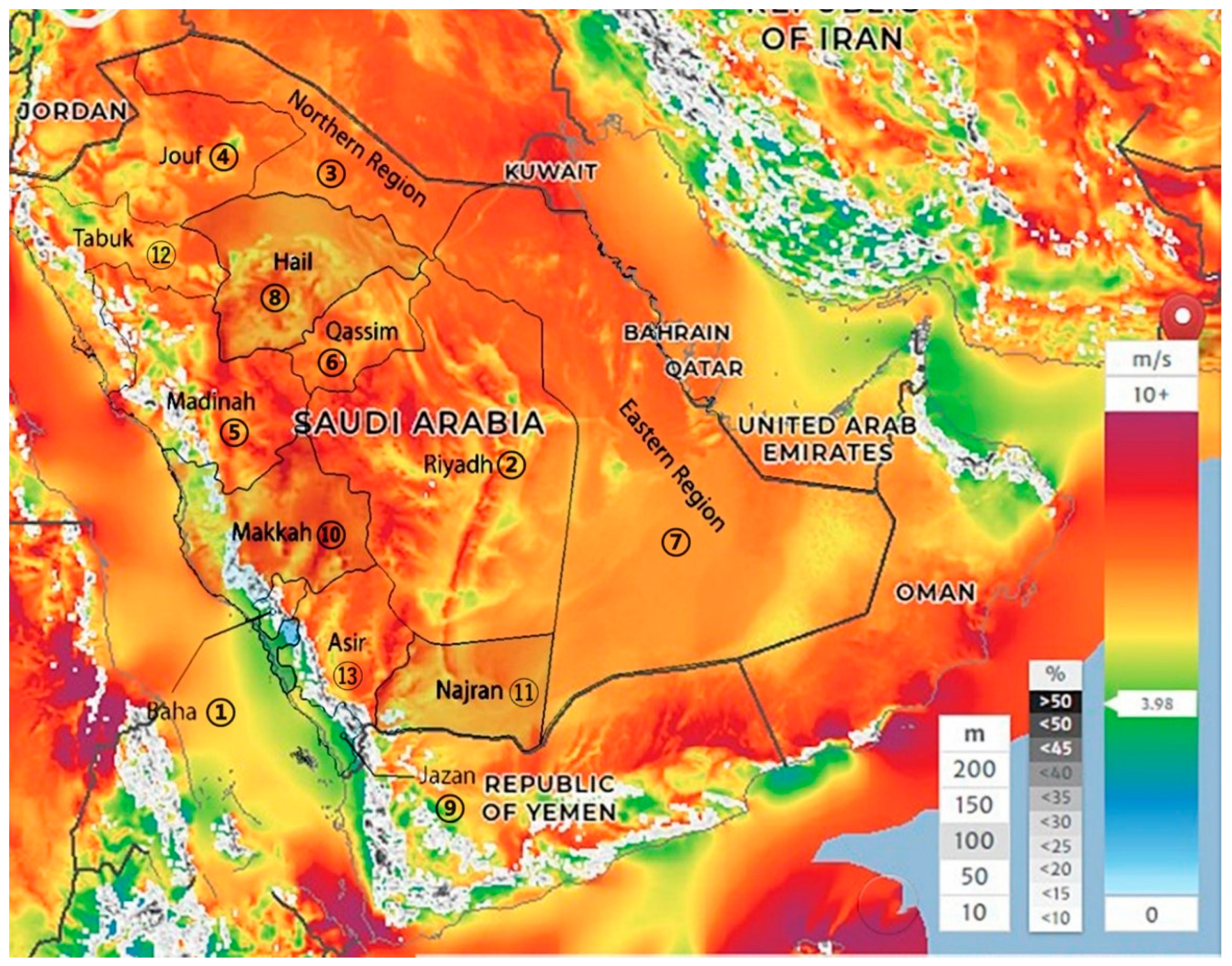
In our analysis, we utilized wind resource data that encapsulate both the average wind power density and average wind speeds across thirteen regions in Saudi Arabia, measured at an altitude of 100 meters. This data spans from 2011 to 2021, offering a decade-long perspective that provides a robust foundation for understanding the temporal stability and geographical variation of wind conditions. The selection of a ten-year period is critical in mitigating the high temporal and geographical variability inherent in wind patterns, thereby ensuring that our assessment reflects both seasonal and annual variations in wind energy potential.
The choice to focus on average wind power density and average wind speeds was driven by the need to provide a stable and representative measure of wind energy potential that accounts for long-term trends rather than short-term fluctuations. These averages are particularly relevant in the regions studied, where, despite the global challenge of wind variability, the temporal and geographical variations are relatively subdued. This lesser variability is attributed to the consistent climatic conditions across these regions, characterized by continued periods of stable and predictable wind patterns. This stability makes averages a reliable metric for assessing wind energy potential in these areas.
The source of wind data was the Saudi Arabian National Center for Meteorology, an entity recognized for its comprehensive and standardized meteorological recordings. This source is deemed reliable due to its systematic and consistent methodology in data collection and its long-standing reputation in climatological research within the region (Saudi Arabian National Center for Meteorology, 2022). Furthermore, the data have been compiled and are presented in Table 6, ensuring transparency and ease of access for further analysis. This systematic presentation aids in the scrutiny and validation of our data utilization approach, reinforcing the justification for the chosen data range and source in capturing the intricacies of wind dynamics pertinent to wind energy projects in Saudi Arabia.
Figure 1.
Wind Speed GIS of Saudi Arabia.
4.3. Explanation of The Selection of Experts for the Rating and Ranking of Wind Locations
We selected a diverse panel of thirty DMs, who have expertise in the energy field and wind energy. Experts’ backgrounds include eDiscovery energy consultants, ACWA Power Saudi Arabia project managers, assistant professors in electrical engineering at King Saud University, renewable energy experts at the Ministry of Energy, and an electrical engineering professor at Al Madinah University. See web supplement VI for list of experts.
4.4. Ranking and Rating of Wind Locations by Thirty Experts
In our experiment, we presented the experts with the list of 13 distinct locations along with their three criteria as presented in Table 6. The experts were asked to rank all locations5 (alternatives) and then to rate each location within 0.01 to 0.99 range where 0.01 is the worst (hypothetical/possible case) and 0.99 is the best (hypothetical/possible ideal case). This detailed process aimed to harness expert judgment in quantifying and prioritizing the potential advantages and disadvantages of each location for wind farm development, ensuring an informed decision-making framework. A sample of the data provided to each DM is shown in the first four columns of Table 6. The corresponding responses by one of experts (we randomly selected expert no. 5) are exhibited in Table 6 in bold in the last two columns.
In this section, we use commonly used average rating of each location using the 30 experts’ responses as shown below. However, in Section 8 of this paper, we will show a more advanced method for combining DMs ratings.
4.5. Normalized Values of Three Criteria to be Used in MCDM Models
5. Experimental Design for Testing MCDM and GDT Models
5.1. Selected MCDM Methods for Comparative Analysis
After preliminary experiments, we selected the following MCDM methods for comparative experiments. These methods were most effective in their given category using the minimum no of parameters.
- (a)
- Linear additive utility function Value function (LV) with no criteria value functions, LV with one value function (LV-1V) for all criteria, and LV with k value functions (LV-kV) for k no. of criteria.
- (b)
- Concave GDT model without any value functions (GDT-1), GDT-1 with one value function (GDT-1-1V), and GDT-1 with k value functions (GDT-1-kV).
- (c)
- Basic GDT (mixed concave/convex) model without any value function (GDT-2), GDT-2 with one value function (GDT-2-1V), and GDT-2 with k value functions (GDT-2-kV).
- (d)
- Keeney multiplicative utility without any value function (SMU), with one value function (MU-1V), and with k value functions (MU-kV).
- (e)
- AHP.
- (f)
- Mean Absolute Deviation-Goal Programming (MAD-GP) (We found that the most effective approach for minimizing to the goal, or the ideal point was MAD-GP).
To reduce the no. of parameters, we considered several simplifications of different models: first, we considered using default values of equal weights; second, for goal values, we considered using default values of equal highest goal, i.e. 0.99 for all goals; third, we considered using no value functions, i.e., v(y) = y for all methods, then using the same one-parameter v(y), Eq. (2.4) for all criteria.
5.2. Validation Process
As discussed before, to validate our results, we used 70% of the data for assessing the parameters of the given model while using the remaining 30% of data for testing the model. Then, we compared the ranking of these 30% of data to those of the DMs. This approach ensures that our conclusions are not based self-prophesy of the training data but is based on external validation of unused data.
5.3. Optimization for Assessing All Models
The general formulation for all models is shown below, where for each model’s utility function, U, given in Table 1, Table 2 and Table 3. Here, is the average of all DMs ratings of location j given in Table 6.
Subject to:
= (utility function of the given MCDM model in Table 1, Table 2 and Table 3) for j = 1, 2, 3, …, n
where represents the positive prediction error (deviation) for alternative j, represents the negative prediction error for alternative j, and n represents the total no. of alternatives.
-1 < z ≤ 0, 0 ≤ zX < 1, (zX – z) ≤ 1.
For example, the optimization formulation for the (GDT-1-1V) model, applied to the 13 MCDM alternatives in Table 7, is presented below, where the right-hand side shows the average ratings from 30 decision-makers for each location.
Subject to:
After solving this problem using an optimization program, we find the solution is: w1=0.5054, w2=0.1959, w3=0.2987, z=-0.99, and α=1 (note α=1 means linear value functions). This is an extremely concave GDT-1 utility function because z=-0.99 is at its extreme value.
5.4. Computation Environment for Optimization for Assessing Parameters of All Models
All optimization problems were run on a personal laptop. The CPU of the used laptop is the 13th Gen Intel(R) Core(TM) i7-13700HX, which can operate at 2.1 GHz by default, but can boost up to 5 GHz. The RAM of the laptop we used is 16 GB. We installed Extended Lingo/Win64 Release 20.0.23 as our software for optimization. The license we have for Lingo (the optimization software) is educational license, which allows us to have unlimited constraints and variables. The default generator memory as 32 MB for the Lingo is enough to run our programs.
6. Results of Using 100% of Data and Comparison of MCDM Methods
6.1. Minimizing the Sum of Squares Error
We employ the sum of squares error (SSE), Eq. (5.1), measuring the deviation between the predicted utility values by the MCDM model vs. the actual assessed utility values by expert DMs.
6.2. MCDM Models and Their Parameters
We consider 28 MCDM models as shown in Table 8. We have formulated each model in accordance with the specifications outlined in Section 5. We used Lingo software to solve each optimization problem (but any other optimization software can also be used). We assess parameters of the given model by minimizing SSE using the same give data set which was used for all models. For example, for GDT-2-kV model, the optimization finds the following parameters: (w1, w2, w3, α1, α2, α3, z, zX).
6.3. Measuring Linear Value Utility Percent Error (LV%)
To compare all different models with respect to a same benchmark, we calculate the LV% error using LV model with equal weights (LV- Equal W), where U = 0.33f1 + 0.33f2 + 0.33f3. Find SSE of this given U for the given data. Then, find SSE of each given model using optimization for the same set of data.
This metric enables us to quantify the relative performance of each MCDM model compared to the baseline of LV with equal weights.
6.4. Assessing of Models Using 100% of Data Set, SSEs, and Their Relative Errors by LV%
Table 8 presents each model along with its no. of parameters. Table 8 also shows SSE of each model, its ranking compared to other models, and its assessed parameters. Note that because in this section, we use 100% of data, models with more parameters generally have smaller SSE and LV% errors. However, we will show in out-of-sample experiments of the next Section, ranking by 100% of data (which is the gold standard in MCDM analysis) provides very inaccurate results.
The SSE values for the best fitting MCDM models using 100% of data for each given no. of parameters is shown in Figure 2 and are explained below.
Zero Parameter: The MCDM model using Equal-W-G is used as the basis for comparison of different models, the LV% of this model is 100%.
One Parameter: The MCDM model Z-MAD-GP-Equal-W-G emerged as the most accurate model fit to the data, delivering the lowest SSE when a single parameter was considered.
Two Parameters: When dealing with two parameters, the model GDT-1-1V-Equal-W outperformed others, displaying the lowest SSE.
Three Parameters: The model GDT-2-1V-Equal-W fit the data, achieving the lowest SSE when the no. of parameters was set to three.
Four Parameters: The model GDT-1-kV-Equal-W fit the data, achieving the lowest SSE when the no. of parameters was set to four.
Five Parameters: The model GDT-2-kV-Equal-W proved to be the best fit to the data, with the lowest SSE, when handling five parameters.
Six Parameters: The model QU-Equal-a&b fit the data, achieving the lowest SSE when the no. of parameters was set to six.
Seven Parameters: For seven parameters, MU-kV was the top-performing MCDM model, exhibiting the lowest SSE.
In general, when using 100% of data, the model associated with the elbow point can be selected. This is the inflection point where models with more parameters have negligible improvements in their SSEs. The selection of elbow point is consistent with choosing a parsimonious model. For example, in Figure 2, GDT-1-kV-Equal-W with four parameters can be recommended because it is associated with the elbow point. However, out-of-sample experiments of the next section, will be needed to verify actually which model is the most accurate for the given set of data.
The model QU with 10 parameters exhibited the best fitting model because it has the lowest SSE for 100% of the data, but in the next section, we will discuss that it is actually the worst model in out-of-sample experiments.
7. Results of 30% Out-of-Sample Data on Randomly Replicas: Validation Process
In this section, we use six replicas of 70% randomly selected data from 100% data set. Here, we have 13 locations, and we used nine randomly selected locations as 70% (to assess parameters of the model) and the remaining four locations as 30% (to test the accuracy of the assessed parameters). Specifically, for each of sex replica, we assess the parameters of each model using its 70% data. Then we used the assessed parameters of each model to measure how accurately the model performs on the remaining 30% of data (which were not used to assess the parameters). Then, we present the average of six replicas for 30% of data. For example, for GDT-2-kV model for the first replica, we used the randomly selected 70% of the data, then we found parameters (w1, w2, w3, α1, α2, α3, z, zX) by minimizing SSE as explained before. Then, we use the obtained parameters to see how accurately these assessed parameters can predict the ratings of the remaining 30% of alternatives which were not used in obtaining the parameters.
7.1. Model Evaluation Based on 30% Out-of-Sample Data
In Table 9, the no. of parameters varies from 1 to 10. The sixth column shows average SSE of six replicas of random samples based on 70% of the data was used to determine the parameters of each model. Then the obtained parameters of different models which were applied to the remaining 30%. Note there are total of nine parameters in all different models: w1, w2, w3, α1, α2, α3, z, zX, and K.
In Table 9, the best-performing model is GDT-1-kV with four parameters. Here this solution means that while the general utility function is a concave function of the three value functions, the first and the third value functions are concave, but the second value function is convex. This solution contradicts the common theoretical understandings in MCDM and decision making that assume value functions and utility functions are concave.
The SSE values for the best-performing MCDM models for the given no. of parameter based on 30% out-of-sample are presented in Figure 3 and Table 9 are explained below. Note that the parameter values given in Table 9 and explained below are based on the first replica; however, Ave SSE and LV% error, and rankings are based on average of seven replicas.
One Parameter: For one parameter, Z-MAD-GP-Equal-W-G model (using parameter z=-0.2956) was the most accurate predictor with the lowest SSE = 0.0153 (LV% error = 19.20%).
Two Parameters: For two parameters, the model GDT-1-1V-Equal-W (using parameter z=-0.8641, α=1.22) outperformed other two-parameter models, where average SSE = 0.0197 (LV% error = 24.72%).
Three Parameters: The model GDT-2-1V-Equal-W (using parameter z=-0.99, zX=0, α=0.001) had average SSE = 0.0299 (LV% error = 37.52%).
Four Parameters: The GDT-1-kV-Equal-W model (using parameter z=-0.862, α1=0.787, α2=3, α3=0.977) had the best performance, attaining the minimum SSE with four parameters where average SSE = 0.0128 (LV% error = 16.06%). Note that this model was ranked 8th when 100% of data was used in Table 8, but here is ranked 1st.
Five Parameters: The model GDT-1-1V (using parameter w1=0.0917, w2=0.7432, w3=0.1651, z=-0.99, α=2) had average SSE = 0.0187 (LV% error = 23.46%).
Six Parameters: The model GDT-2-1V (using parameter w1=0.001, w2=0.8782, w3=0.1208, z=-0.9181, zX=0.0533, α=2.062) had average SSE = 0.0196 (LV% error = 24.59%).
Seven Parameters: GDT-1-kV (using parameter w1=0.0568, w2=0.8296, w3=0.1136, z=-0.9051, α1=0.001, α2=3, α3=3) had average SSE = 0.0239 (LV% error = 29.99%)
Ten Parameters: For ten parameters, the QU MCDM model exhibited the highest average SSE = 0.1534 (LV% error = 192.47%).
7.2. Discussion of the Best MCDM Method and Its Application to Wind Farm Problem
The best model for the data used in this paper is GDT-1-kV-Equal-W; this model uses equal weights (as default values) and k value functions plus z having a total of k+1 parameters (in this application k+1=3+1=4) parameters. In out-of-sample experiments of six randomly selected replicas, this model has the best (the minimum) SSE of 0.0128 (where LV% error = 16.06%). The parameters of most replicas were similar for GDT-1-kV-Equal-W model, for example in one replica, z = -0.862, α1 = 0.787, α2 = 3, α3 = 0.977, where the given default values of w1 = 0.333, w2 = 0.333, w3 = 0.333 were used6. This solution has profound meanings which cannot be easily found using classical MCDM methods. Here, the weights of importance are not critical (using default equal weights); however, we can observe that although all criteria are increasing but they have different meanings. For first criterion, α1 = 0.787 where value function, v(f1), is concave (in average wind density) meaning diminishing in return. For the second criterion, α2 = 3 where v(f2) is highly convex (in average wind speed) meaning increasing in return. And for the third criterion v(f3), α3 = 0.977, is concave but almost linear (in conducive terrain) meaning almost constant in return. Now, we explain the meaning of z = -0.862, this means that the Utility function, U, is highly concave in (v(f1), v(f2), v(f3)); which is consistent with economical models preferring non-extreme points to extreme points; however, v(f2) is convex; this results in a mixed concave/convex utility function. Furthermore, here, we observe that assessing utility functions by direct ranking and rating of alternatives is far superior in out-of-sample experiments than those MCDM methods that assess the parameters of the utility function directly (not using real alternatives (e.g., assessing additive MAUFs parameters and also the direct assessment of weights of importance as is done in AHP).
Applying this GDT model resulted in the ranking of locations as: 1. Tabuk, 2. Baha, 3. Najran, 4. Northern region, 5. Asir, 6. Madinah, 7. Makkah, 8. Hail, 9. Jouf, 10. Riyadh, 11. Eastern Region, 12. Qassim and 13. Jazan regions.
8. Discussion of Group Decision Making and Its Resolution by New MCDM-GDT
In the application to wind-farm location selection, we used the average of ratings of 30 experts (DMs) for each given alternative (location). The problem of using average of ratings is that it is linear and does not consider the deviation of different DMs’ ratings. Here, we provide an extension based on MCDM-GDT that gives more credit to the majority of DMs who are more consistent in their ratings with each other while extreme ratings are less credited. We do this by using GDT-1 model which is a concave function7. We have not found any papers in the literature addressing this issue of nonlinear aggregations of DMs’ ratings; however, for a technical approach to this problem see López-Morales (2018) and for a broader approach see Davey, Ann, and David Olson (1998).
In this section we apply MCDM-GDT approach for aggregating multiple DMs’ ratings of different alternatives. Suppose that there are n alternatives for j = 1, 2, …, n and Q no of DMs for q = 1, 2, …, Q. Suppose that is the rating value of alternative (e.g. location) j given by DM no. q (DMq) where ratings are normalized form of 0.01 to 0.99.
Suppose that is the importance given to the DMq where . Using these weights, we can define the LV of multiple DMs in Eq. (8.1). LV is a simple composite approach based on weighted rating of multiple DMs.
Here, LV is a weighted linear function. When weights are equal, this function is the same as average function. LV may result in incorrect ratings of locations because the ratings of some DMs could be substantially different from others. That is, the varying priorities inherent in data from distinct (out of normal range) DMs may hold greater significance on the LV values of different alternatives. Relying on LV disregards the proper consideration of dispersion of the data; for example, two alternatives with equivalent LV may have substantially differing levels of dispersion. We propose to measure and use these dispersions for the proper ranking of alternatives using MCDM-GDT applied to the multiple DMs problem. This model incorporates dispersions of different DMs; such that more priority will be given to DMs who are more consistent with each other (those who have more similar ratings). First, we define the geometric value (GV) for the multiple DMs problem.
GV is a concave function of consequences without using any parameters. As dispersion of decreases, GV approaches LV; when all are the same, GV = LV.
Now, we can define geometric deviation (GD) for each alternative as the difference between LV and GV.
GD approaches 0 as dispersion decreases. The aggregate utility of multiple DMs based on GDT is defined as:
where -1 < z ≤ 0. This satisfies the first-order stochastic principle in risk problems (Malakooti, 2018, 2024; Malakooti et al., 2021); and it also satisfies non-dominancy (efficiency) for the multiple DMs problem. It is evident that the z-value represents the degree of emphasis on dispersion by the DMs; a smaller z (towards -1) indicates a greater emphasis on minimizing dispersions. That is, using z = 0 implies that dispersions of different DMs do not matter, and using z = -0.99 means that dispersions matter, such that the effect of extreme DMs is minimized. Theoretically, z cannot be lower than -1 because the solution can be inefficient (dominated) (Malakooti, 2018, 2024; Malakooti et al., 2021).
One can suggest using standard deviation (SD), as in mean-variance, to measure dispersion instead of GD used in GDT. However, mean-variance violates first-order stochastic dominance (and here the dominancy or efficiency principle; see K. Borch, 1969). This means that using SD might lead to selecting dominated points. Conversely, utilizing GD can uphold first-order stochastic dominance. A small example is presented below to show this concept. For example, suppose that we have four DMs and two locations. The four DMs have rated location a1 as 0.99, 0.8, 0.7, and 0.7, and location a2 as 0.9, 0.8, 0.7, and 0.7, respectively. Here, we assume the weights of importance of all DMs are the same, i.e., = 0.25 for all for q = 1, 2, 3, 4. See Table 10.
Note that is dominated by based on the non-dominancy (efficiency) principle. However, using SD here results in selecting which is a dominated alternative.
Now, we apply, the multiple DMs GDT approach to the wind location problem. In the wind farm selection, we have n = 13 locations and Q = 30 DMs. First, we assume that we assume the weights of importance of all DMs are the same, i.e. = 1/30 for q = 1, 2, 3, …, 30. Also, we use z = -0.99 to give more importance to similar ratings closer to the average. According to Table 11, Tabuk is the best and Jazan is the worst alternative.
For this application, the ranking of locations remains the same across different z values, from 0 to -0.99. These results indicate that most experts in our experiment exhibit minimal dispersion in their ratings, thus, their differences have little impact on the rankings. Their ratings closely align with one another, reflecting their expert opinions.
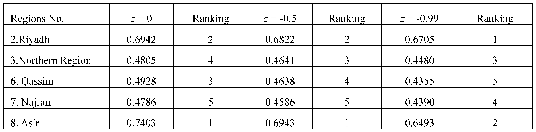
Nevertheless, to demonstrate an example that the rankings will change depending on alternatives and DMs, in the following, we select ratings from 10 experts (out of 30) who have the largest dispersion with each other and apply them to five locations that also have the most dispersions. Again, we assign equal weights for DMs, i.e., . The aggregate utility values are presented in the table below, demonstrating how the rankings shift with varying z-values. See Table 12 that shows for z = -0.99, Riyadh is no. 1, and Asir is ranked as no. 2, while for z = 0, these ranks are reversed.
The regions presented in Table 12 demonstrate how rankings of alternatives may change as z changes. Looking at regions Riyadh, Asir, Northern Region, Qassim, and Najran, we can see ranking changes from using z = 0 (not using dispersions) and z = -0.99 (using dispersions such that the effect of extreme DMs is minimized). The average aggregate does not consider the dispersion in ratings, but GDT will account for those disparities.
9. Conclusions and Future Work
Although the idea of sample vs. out-of-sample testing for validating models is well-known in the literature, but in this paper, for the first time, we provided its application for evaluating and ranking MCDM methods based on real-world experiments. We applied this approach for rating MCDM alternative wind farm locations for the renewable energy sector in Saudi Arabia. Using sample vs. out-of-sample, we evaluated several well-known MCDM methods including our newly developed MCDM-GDT model.
In this paper, we developed, MCDM-GDT method by adopting the ideas of a risk model called Risk-GDT which was developed by (Malakooti 2018, 2024; Malakooti et al., 2021). Special cases of MCDM-GDT include important MCDM models such as additive, multiplicative, concave & convex functions. To simplify, the assessment process, we showed its different parametric special cases by using default values of parameters. MCDM-GDT has (2k+2) parameters. However, it can be simplified to one parameter by using default values. We illustrated that how to find the parsimonious MCDM-GDT model with the least no. of parameters to solve and analyze a given MCDM problem. We start by one parameter (using z) and start going up one parameter at a time up to (2k+2) parameters. Based on out-of-sample experiments, for this application of wind location, we found that k+1 parameters were sufficient to assess the best fitting model: GDT-1-kV (see Table 4). This model is a mixed concave/convex function where the utility function is a concave function of three criteria value functions, but the second criterion has a convex value function while the other two value functions were concave. We suggested that this is surprising result that contradicts theoretical assumptions in MCDM and decision making which assume concavity is underlying behavior. Overall, for the same no. of parameters, different special cases of MCDM-GDT outperformed other MCDM models.
For wind location problem in Saudi Arbia, we developed the objective measurements (metric) of three criteria for the evaluation of thirteen locations. We used the ratings of the 30 experts for the wind locations and then applied sample vs. out-of-sample MCDM approach to select the best location.
Furthermore, we also develop a nonlinear aggregation of experts’ ratings based on MCDM-GDT and ranked alternatives. This MCDM-GDT model for aggregating experts’ assessment is also new to the literature; and it has the advantage of minimizing the effects of extreme opinionated experts while not eliminating their opinions.
Future research in this area can include experiments with additional real-world datasets and with a variety no. of criteria and alternatives. Also, one can consider exploring the performance of other MCDM models in out-of-sample experiments and compare them to MCDM-GDT. For other renewable energy problems, we suggest considering the identification and quantification of appropriate criteria and the application of MCDM methods for evaluating energy saving alternatives. We also proposed a generalization of MCDM-GDT model (Eq. 3.16) which includes also minimizing distance to idea points and maximizing distance to nadir points; this model can be further investigated.
Supplementary Materials
The following supporting information can be downloaded at the website of this paper posted on Preprints.org.
Abbreviation
| SSE | Sum of Squares Error |
| wi | Weights of importance of criteria i where i=1, 2, …, k |
| fij | Normalized value of (actual value) for criteria i and alternative j |
| Fj | Normalized value of all criteria for alternative j where j=1, 2, …, n |
| vi(fi) | Value function of criteria i |
| αi | Parameter of power value function vi(fi) |
| LV | Linear Value Utility function |
| AHP-LV | Linear Value Utility function using AHP—process to assess weights |
| LV-kV | Additive Linear Value Utility using k different value functions |
| LV-1V | Additive Linear Value Utility using one value function |
| MU-kV | Keeney: Multiplicative Utility functions using k different value functions vi(fi) = |
| SMU | Keeney: Simplified Multiplicative- Utility function where vi(fi) = fi |
| MAD-GP-General | Weighted Mean Absolute Deviation-Goal Programming (MAD-GP); for default values of 0.99 are used |
| Z-MAD-GP | Z-Goal Programming (Malakooti (2014, pp.99-108)) |
| QU | Quadratic Utility function (shown for three criteria, k = 3) |
| GV | Geometric Value function (GV ≤ LV) |
| GD | Geometric Dispersion function |
| GDT-1 | Geometric Dispersion Theory model |
| XV | X-geometric Value function (LV ≤ XV) |
| XD | X-geometric Dispersion function |
| GDT-2 | Basic Geometric Dispersion Theory model |
| LVG-kV | Linear function with k value function |
| GVG-kV | Geometric Value with k value function |
| GDG-kV | Geometric Deviation Value with k value function |
| XVG-kV | X-geometric Value with k value function |
| XDG-kV | X-geometric Deviation Value with k value function |
| GDT-1-kV | GDT-1 with k different value functions |
| GDT-2-kV | GDT-2 with k different value functions |
| LVG-1V | Linear function with one value function |
| GVG-1V | Geometric Value with one value function |
| GDG-1V | Geometric Deviation Value with one value function |
| XVG-1V | X-geometric Value with one value function |
| XDG-1V | X-geometric Deviation Value with one value function |
| GDT-1-1V | GDT-1 with one different value functions |
| GDT-2-1V | GDT-2 with one different value functions |
References
- Bezadian, M.; Kazemzadeh, R.; Albadvi, A.; Aghdasi, M. PROMETHEE: A Comprehensive Literature Review on Methodologies and Applications. Eur J Oper Res, 2010, 200(1), pp. 198–215. [CrossRef]
- Brauers, W.K.M. and Zavadskas, E.K. Project management by MULTIMOORA as an instrument for transition economies. Technological and economic development of economy, 2010, 16(1), pp.5-24. [CrossRef]
- Cavallaro, F.; Ciraolo, L. Multicriteria Approach to Evaluate Wind Energy Plants on an Italian Island. Energy Policy, 2005, 33, 235–244. [CrossRef]
- Ceballos, B., Lamata, M.T. and Pelta, D.A. A comparative analysis of multi-criteria decision-making methods. Progress in Artificial Intelligence, 2016, 5, pp.315-322. [CrossRef]
- Chen, S.J. and Hwang, C.L.. Fuzzy multiple attribute decision making methods. In Fuzzy multiple attribute decision making: Methods and applications, 1992, (pp. 289-486). Berlin, Heidelberg: Springer Berlin Heidelberg. [CrossRef]
- Colapinto, C., Jayaraman, R. & Marsiglio, S. Multi-criteria decision analysis with goal programming in engineering, management and social sciences: a state-of-the art review. Ann Oper Res 251, 7–40 (2017). [CrossRef]
- Davey, A.; Olson, D. Multiple Criteria Decision Making Models in Group Decision Support. Group Decis Negot, 1998, 7, pp. 55–75. [CrossRef]
- Eintalu, J. Utility Function u = x/(x + 1); Lambert Academic Publishing: London, UK, 2019. ISBN 978–620–0–30723–1.
- Ehrgott, Matthias. Multicriteria optimization. Vol. 491. Springer Science & Business Media, 2005. [CrossRef]
- González, J.S.; Gonzalez, A.; Mora, J.C.; Santos, J.M.R.; Payan, M.B. Optimization of Wind Farm Turbines Layout Using an Evolutive Algorithm. Renew Energy, 2010, 35, pp. 1671–1681. [CrossRef]
- Hou, P., Hu, W., Soltani, M., Chen, C., Zhang, B. and Chen, Z., 2016. Offshore wind farm layout design considering optimized power dispatch strategy. IEEE Transactions on sustainable energy, 8(2), pp.638-647. [CrossRef]
- Hwang, G.H.; Wei, L.S.; Ching, K.B.; Lin, N.S. Wind Farm Allocation in Malaysia Based on Multi-Criteria Decision Making Method. 2011 National Postgraduate Conference, Perak, Malaysia, 2011, pp. 1-6. [CrossRef]
- Jacquet-Lagreze, E.; Siskos, J. Assessing a Set of Additive Utility Functions for Multicriteria Decision-Making, the UTA Method. Euro J Op Res, 1982, 10, pp. 151–164. [CrossRef]
- Kahraman, C.; Ruan, D.; Doğan, D.A. Comparative Analysis of Multiple Criteria Decision Making Methods with Respect to Sustainable Solid Waste Management in Istanbul. Waste Manag, 2003, 23, pp. 345-358. [CrossRef]
- Keeney, R.L. Multiplicative Utility Functions. Oper Res, 1974, 22, pp. 22-34. [CrossRef]
- Keeney, R.L. A Decision Analysis with Multiple Objectives: The Mexico City Airport. The Bell Journal of Economics and Management Science, 1973, 4, pp. 101–17. [CrossRef]
- Keeney, R.L. and Raiffa, H., 1993. Decisions with multiple objectives: preferences and value trade-offs. Cambridge university press. [CrossRef]
- Klein, G., Moskowitz, H., Mahesh, S., & Ravindran, A. (1985). Assessment of multiattributed measurable value and utility functions via mathematical programming. Decision Sciences, 16(3), 309-324. [CrossRef]
- Komaki, M.; Malakooti, B. Geometric Dispersion Theory for Portfolio Accurate Out-of-Sample Predictions of Stock Market. SSRN Papers, 2019. [CrossRef]
- Lee, A.H.I.; Chen, H.H.; Kang, H.-Y. Multi-criteria Decision Making on Strategic Selection of Wind Farms. Renew Energy, 2009, 34, pp. 120-126. [CrossRef]
- López-Morales, V. Multiple Criteria Decision-Making in Heterogeneous Groups of Management Experts. Information 2018, 9, 300. [CrossRef]
- Malakooti, Behnam. Operations and Production Systems with Multiple Objectives; Wiley-Interscience, 2014. ISBN-13: 978-0470037324.
- Malakooti, B. (2015). Double Helix Value Functions, Ordinal/Cardinal Approach, Additive Utility Functions, Multiple Criteria, Decision Paradigm, Process, and Types (Z Theory I). International Journal of Information Technology & Decision Making, 14(06), 1353-1400. [CrossRef]
- Malakooti, B. Out-of-Sample Predictions of CPT and Geometric Dispersion Theory of Descriptive Choice Under Risk, Empirical Testbeds, Paradoxes, and Risk Triad, June 5, 2018, https://ssrn.com/abstract=3193116.
- Malakooti, B.; Komaki, M.; Al-Najjar, C. Basic Geometric Dispersion Theory of Decision Making Under Risk: Asymmetric Risk Relativity, New Predictions of Empirical Behaviors, and Risk Triad. Decision Analysis, 2021, 18(1), pp. 1-99. [CrossRef]
- Malakooti, B. Geometric Dispersion Theory of Decision Making under Risk: Out-of-Sample Predictions, Paradoxes, Four Types of Risk Patterns, Generalizing Expected Utility, Rank Dependent Utility, & Cumulative Prospect Theory Working paper, Case Western Reserve University, Cleveland, OH, 2024 (to appear in papers.ssrn.com).
- Malakooti, B., A. Altowriji, , H. Wang, Web Supplement of MCDM-GDT Wind Farm , https://www.dropbox.com/scl/fo/lh73lcgv16semyt6908c5/ABCs7GMYmFE8TYIR0DVjSqM?rlkey=9adj2pqfa8hao13r6tidy0nu4&st=4wqieazk&dl=0.
- Manousakis, N.M., Psomopoulos, C.S., Ioannidis, G.C. and Kaminaris, S.D., 2021. A Binary Integer Programming Method for Optimal Wind Turbines Allocation. Clean Technologies, 3(2), pp.462-473. [CrossRef]
- Mostafaeipour, A.; Mostafaeipour, N. Renewable Energy Issues and Electricity Production in Middle East Compared with Iran. Renew Sustain Energy Rev, 2009, 13(6-7), pp. 1641-1645. [CrossRef]
- National Center of Meteorology. Surface Combination of Yearly Climatological Report from 2012-2021. https://www.ncm.gov.ae/resources/climate-reports/ncm-annual-climate-assessment-2022-s.pdf.
- Nematollahi, O.; Hoghooghi, H.; Rasti, M.; Sedaghat, A. Energy Demands and Renewable Energy Resources in the Middle East. Renew Sustain Energy Rev, 2016, 54, 1172-1181. [CrossRef]
- Opricovic, S. and Tzeng, G.H. Compromise solution by MCDM methods: A comparative analysis of VIKOR and TOPSIS. European journal of operational research, 2004, 156(2), pp.445-455. [CrossRef]
- Saaty, T. Decision Making with the Analytic Hierarchy Process. Int J Services Sciences, 2008, 1(1),pp 83-98. [CrossRef]
- Saaty, T.L. Rank from Comparisons and from Ratings in the Analytic Hierarchy/Network Processes. Eur J Op Res. 2006, 168, pp. 557-570. [CrossRef]
- Saaty T. The Analytic Hierarchy Process: Planning, Priority Setting, Resource Allocation; McGraw-Hill: New York, NY, USA, 1980. ISBN-13: 978-0070543713.
- Tamiz, M., Jones, D.F. & El-Darzi, E. A review of Goal Programming and its applications. Ann Oper Res 58, 39–53 (1995). [CrossRef]
- Tamiz, M., Jones, D. and Romero, C. Goal programming for decision making: An overview of the current state-of-the-art. European Journal of operational research, 1998, 111(3), pp.569-581. [CrossRef]
- Tsoutsos, T.; Drandaki, M.; Frantzeskaki, N.; Iosifidis, E.; Kiosses, I. Sustainable Energy Planning by Using Multi-Criteria Analysis Application in the Island of Crete. Energy Policy, 2009, 37, pp.1587-1600. [CrossRef]
- Wan, C., Wang, J., Yang, G. and Zhang, X., 2010. Optimal micro-siting of wind farms by particle swarm optimization. In Advances in Swarm Intelligence: First International Conference, ICSI 2010, Beijing, China, June 12-15, 2010, Proceedings, Part I 1 (pp. 198-205). Springer Berlin Heidelberg. [CrossRef]
- Zavadskas, E.K.; Turskis, Z.; Kildienė, S. State of Art Surveys of Overviews on MCDM/MADM Methods, Technological and Economic Development of Economy, 2014, 20, pp. 165-179. [CrossRef]
- Zeleny, M. Multiple Criteria Decision Making; McGraw Hill: New York, NY, USA, 1982. ISBN- 9780070727953.
Figure 2.
Using 100% of the data. SSE for the best 10 MCDM Models. The no. of Parameters Range From 0 to 8, and then 10; They are Shown in Parentheses After Each Model Name. .
Figure 2.
Using 100% of the data. SSE for the best 10 MCDM Models. The no. of Parameters Range From 0 to 8, and then 10; They are Shown in Parentheses After Each Model Name. .
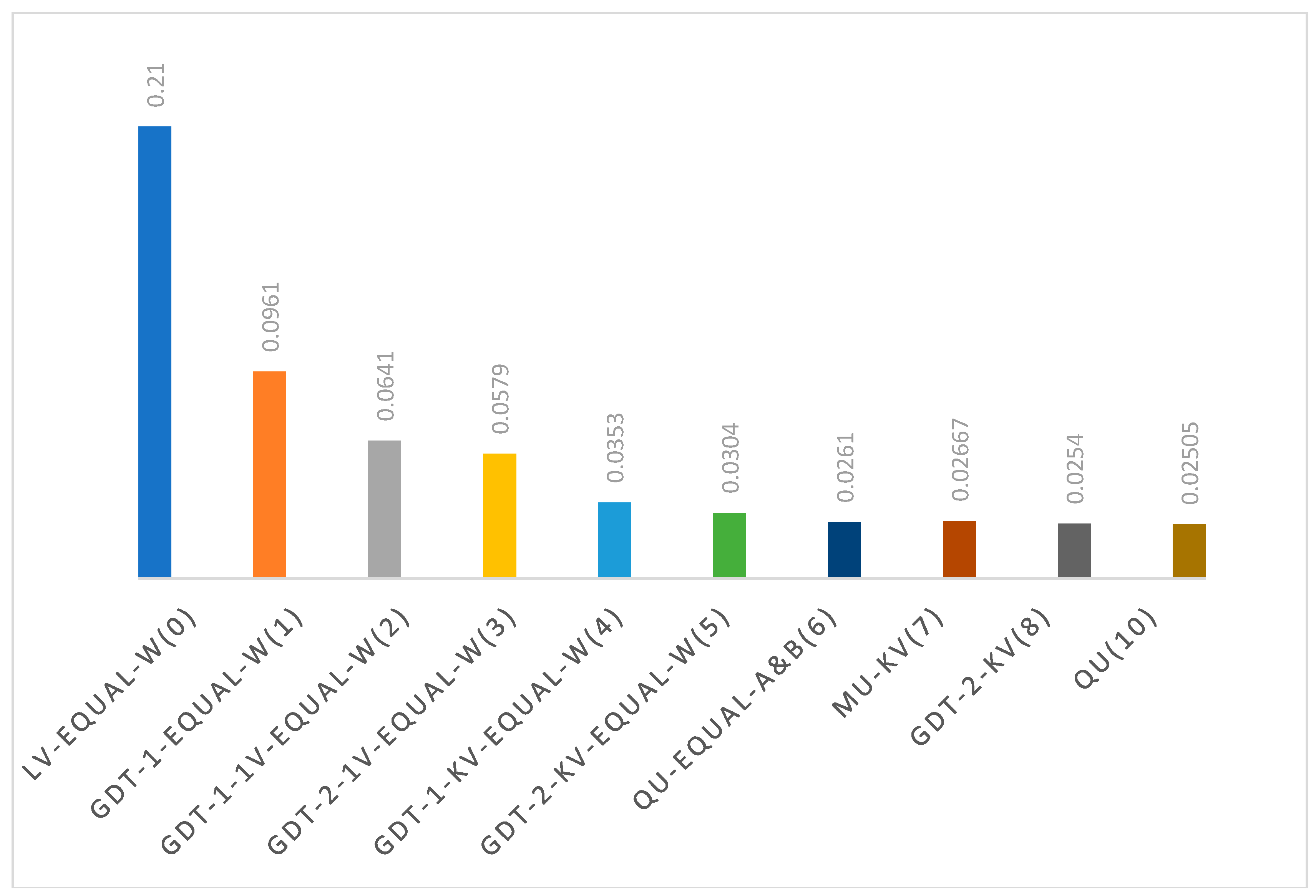
Figure 3.
Average SSE of Six Replicas for 30% Out-Sample Experiments. Top Ten MCDM Models for The Given No. of Parameters in Parentheses are shown.
Figure 3.
Average SSE of Six Replicas for 30% Out-Sample Experiments. Top Ten MCDM Models for The Given No. of Parameters in Parentheses are shown.
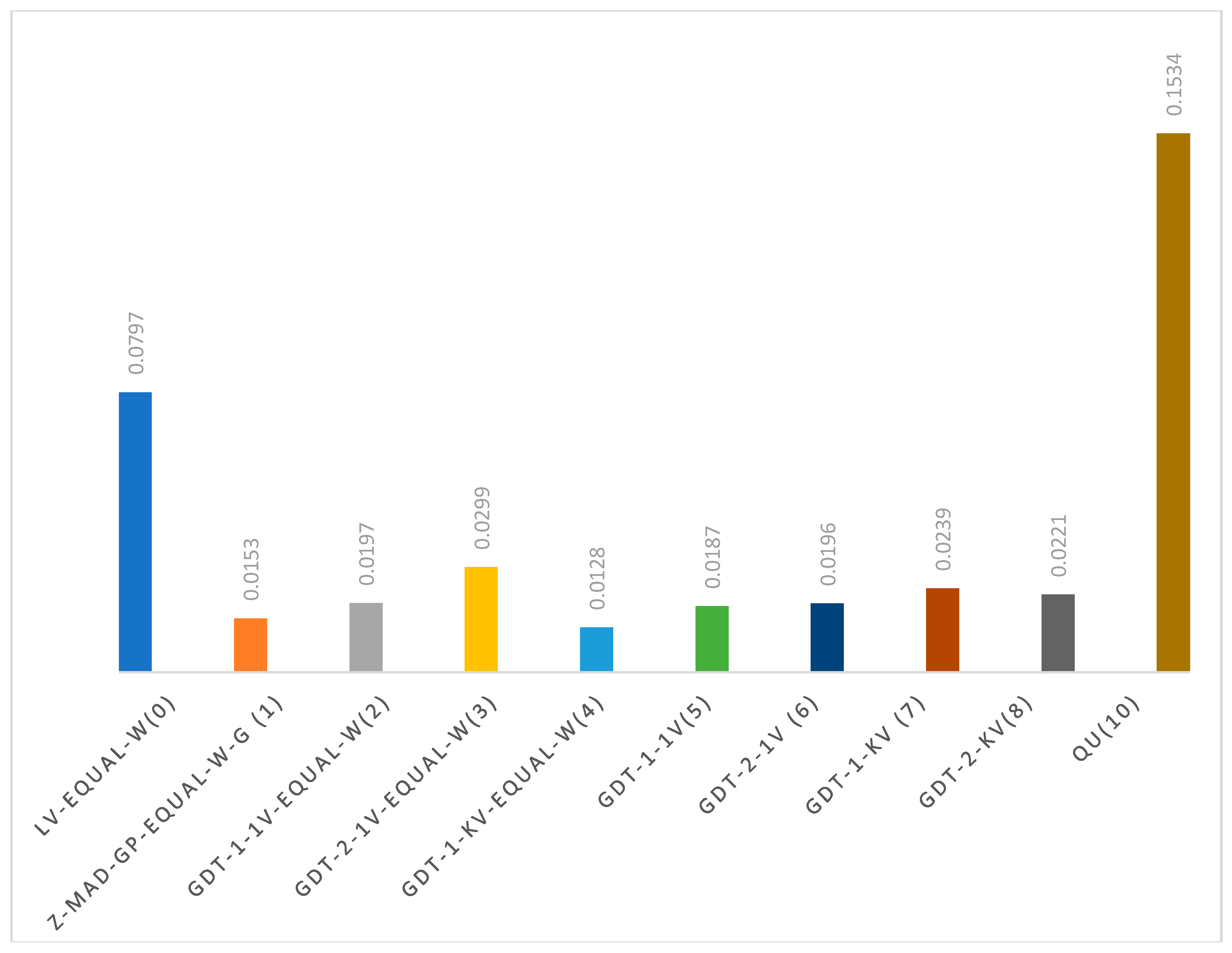

Table 1.
A Summary of Some Important MCDM Models Used in This Paper for Comparative Analysis.
Table 2.
Summary of Basic MCDM-GDT where v(fi)=fi for all i.
Table 3.
Summary of MCDM-GDT with value functions where v(fi)= for all i.
Table 4.
A Flow-chart of Instruction of Choosing One of 12 MCDM-GDT with the Minimum no. of Parameters. Each Cell Shows: Order of easiness (total no. of parameters)), Parameters, & Eq. No.
Table 4.
A Flow-chart of Instruction of Choosing One of 12 MCDM-GDT with the Minimum no. of Parameters. Each Cell Shows: Order of easiness (total no. of parameters)), Parameters, & Eq. No.
Table 5.
Terrain Suitability Assessment of Thirteen Locations.
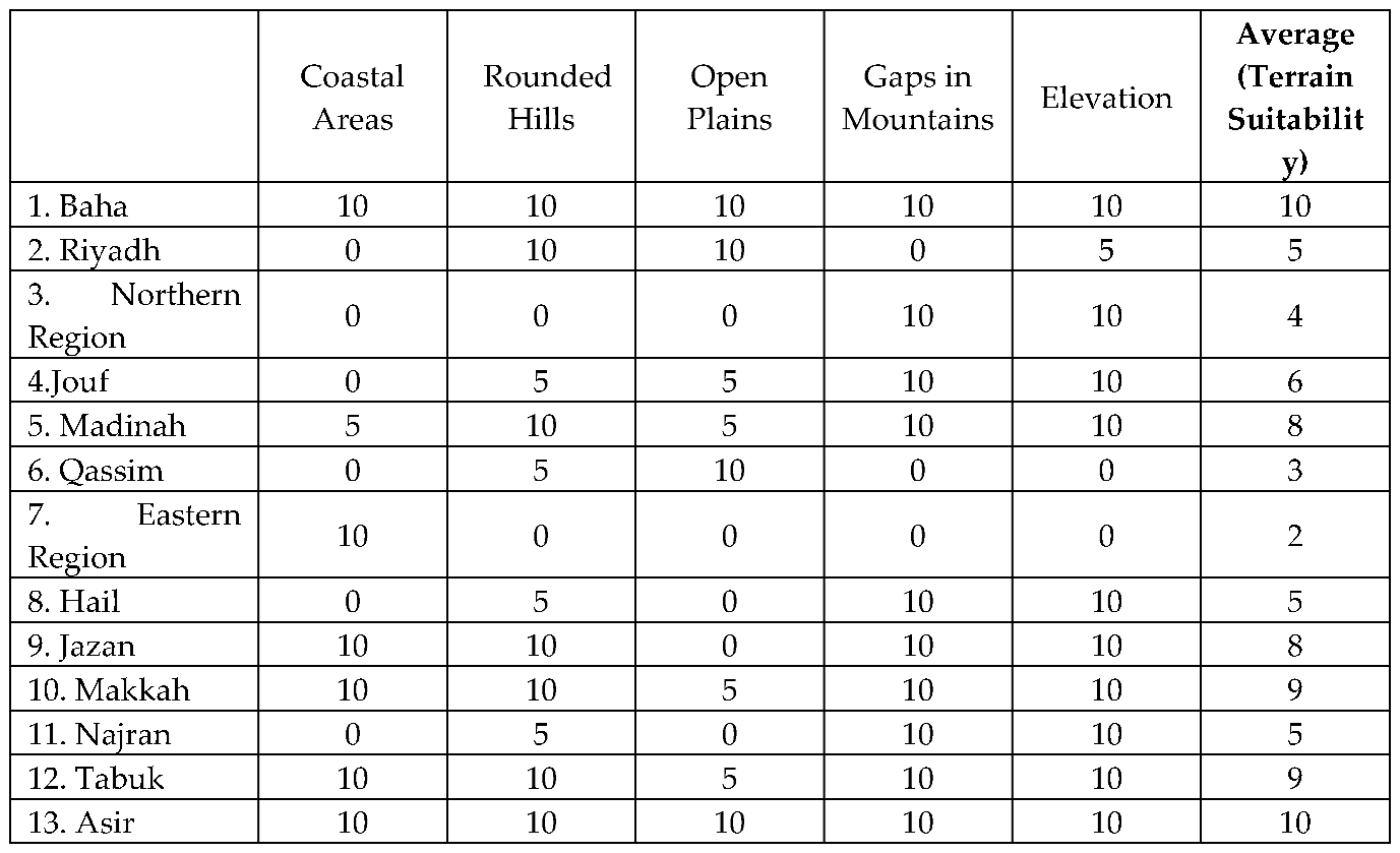
Table 6.
Data Provided to All Experts: Response of One Expert is Shown in the Last Two Columns.
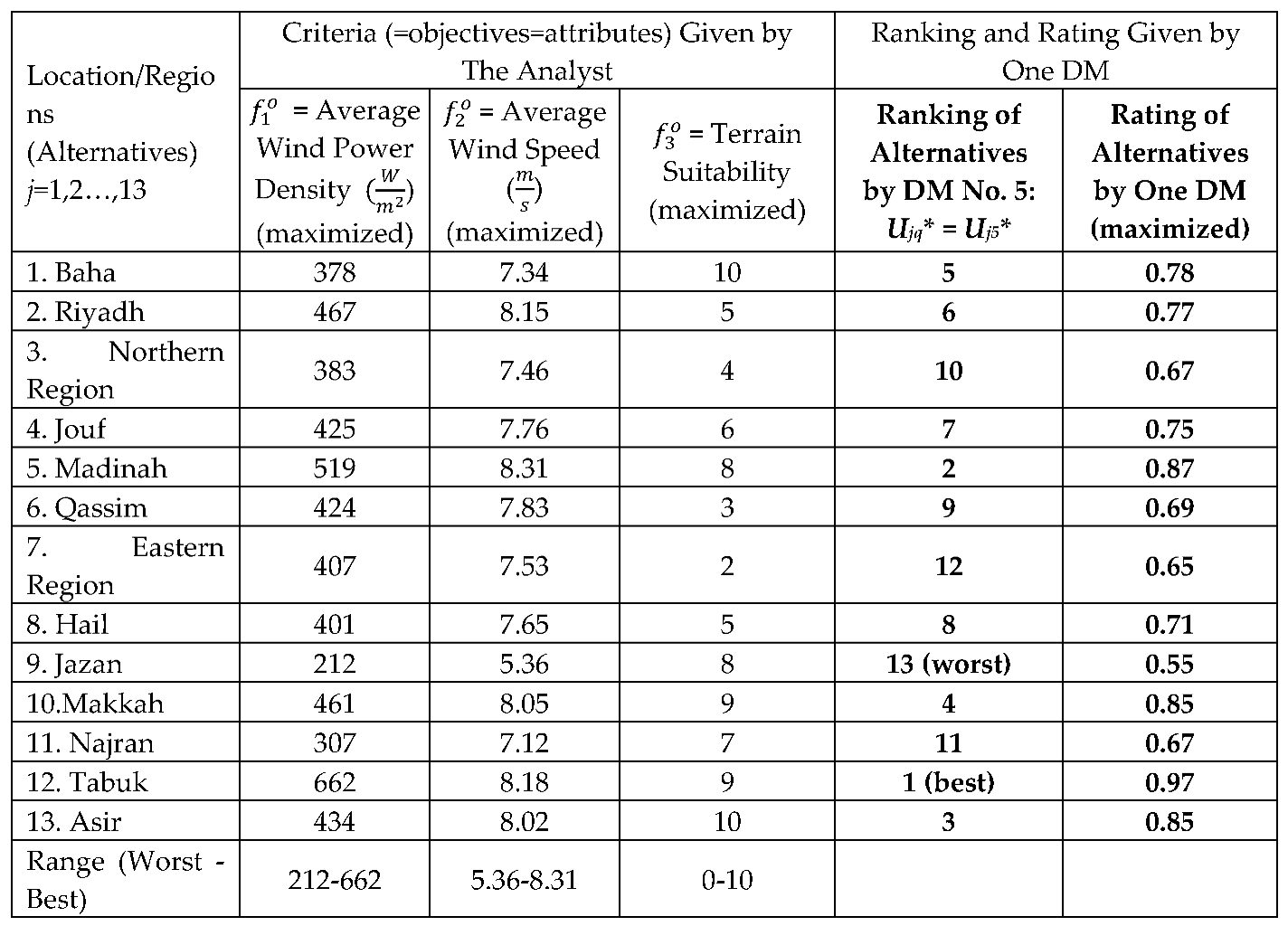
Table 7.
Saudi Arabia Regions Normalized Criteria to Be Used in MCDM Models.
Table 8.
The SSE, LV% error, and the assessed parameters of each MCDM model using 100% of data and testing the model on the same 100% of data.
Table 8.
The SSE, LV% error, and the assessed parameters of each MCDM model using 100% of data and testing the model on the same 100% of data.
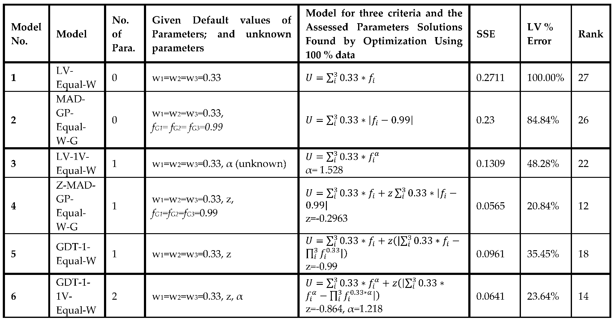
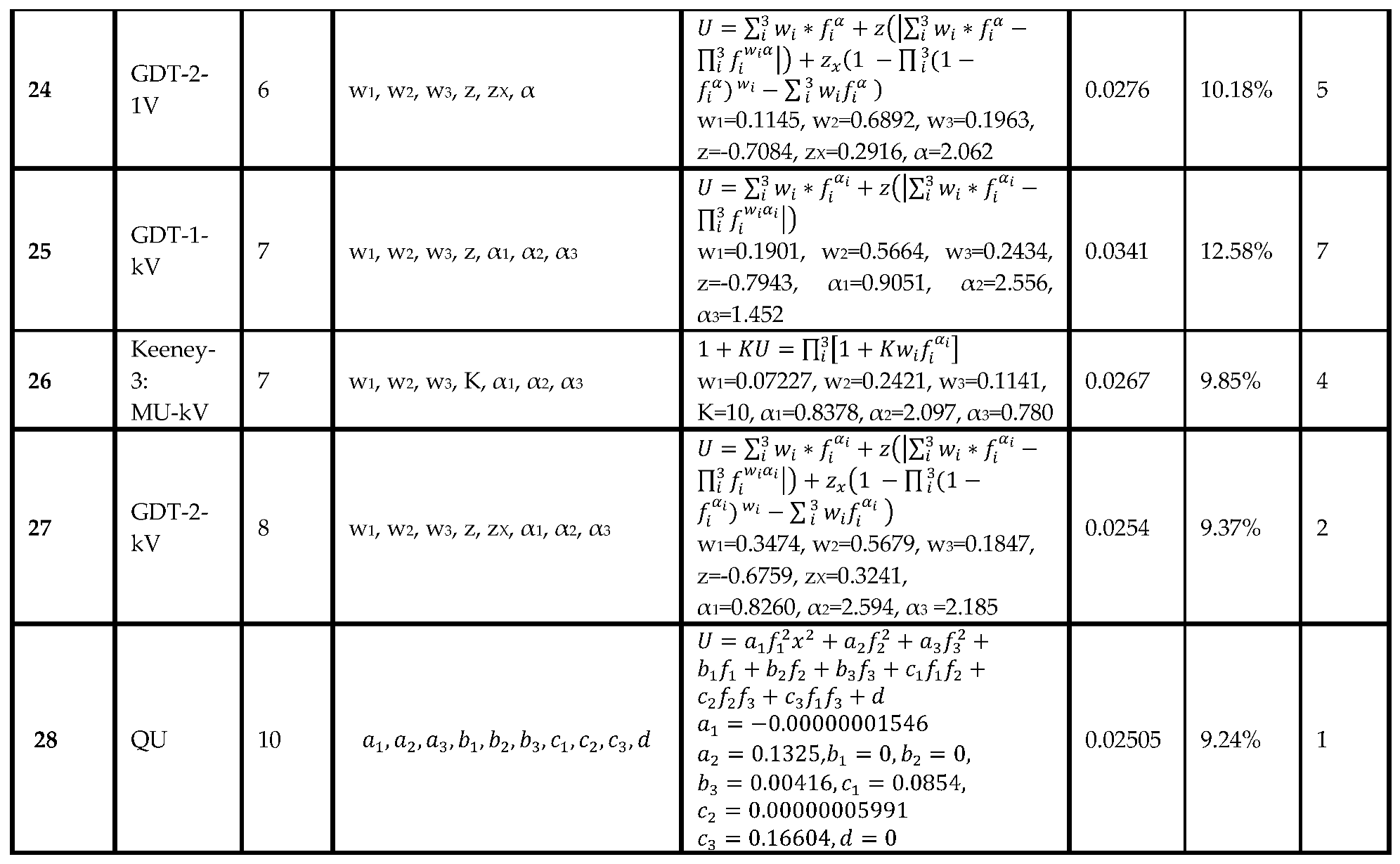
Table 9.
Average Accuracy of Six Replicas of 30% of Out-of-Sample: Using SSE to Compare MCDM Models where Parameters of Each Model was Obtained from its 70% Training data (In-sample).
Table 9.
Average Accuracy of Six Replicas of 30% of Out-of-Sample: Using SSE to Compare MCDM Models where Parameters of Each Model was Obtained from its 70% Training data (In-sample).
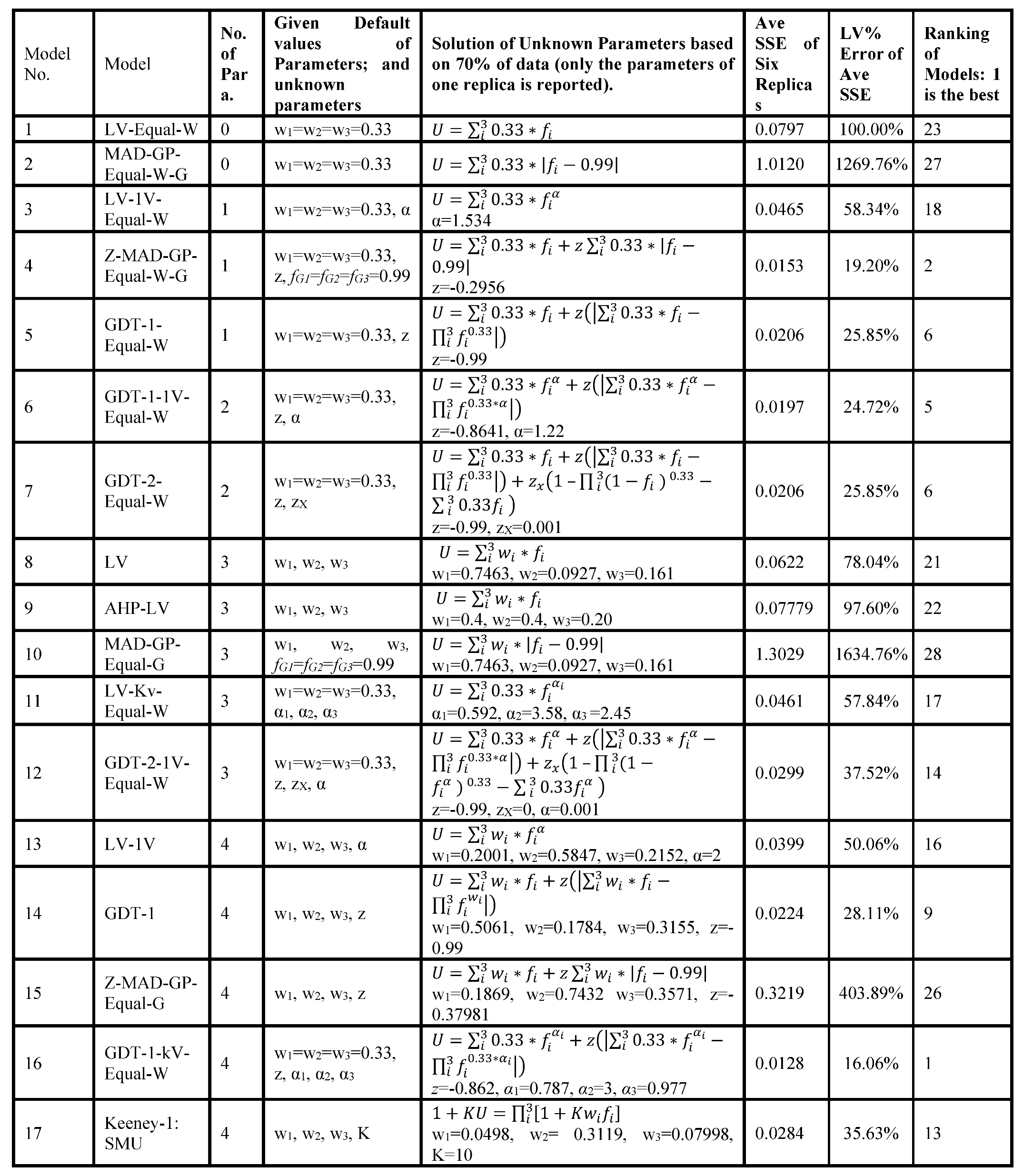
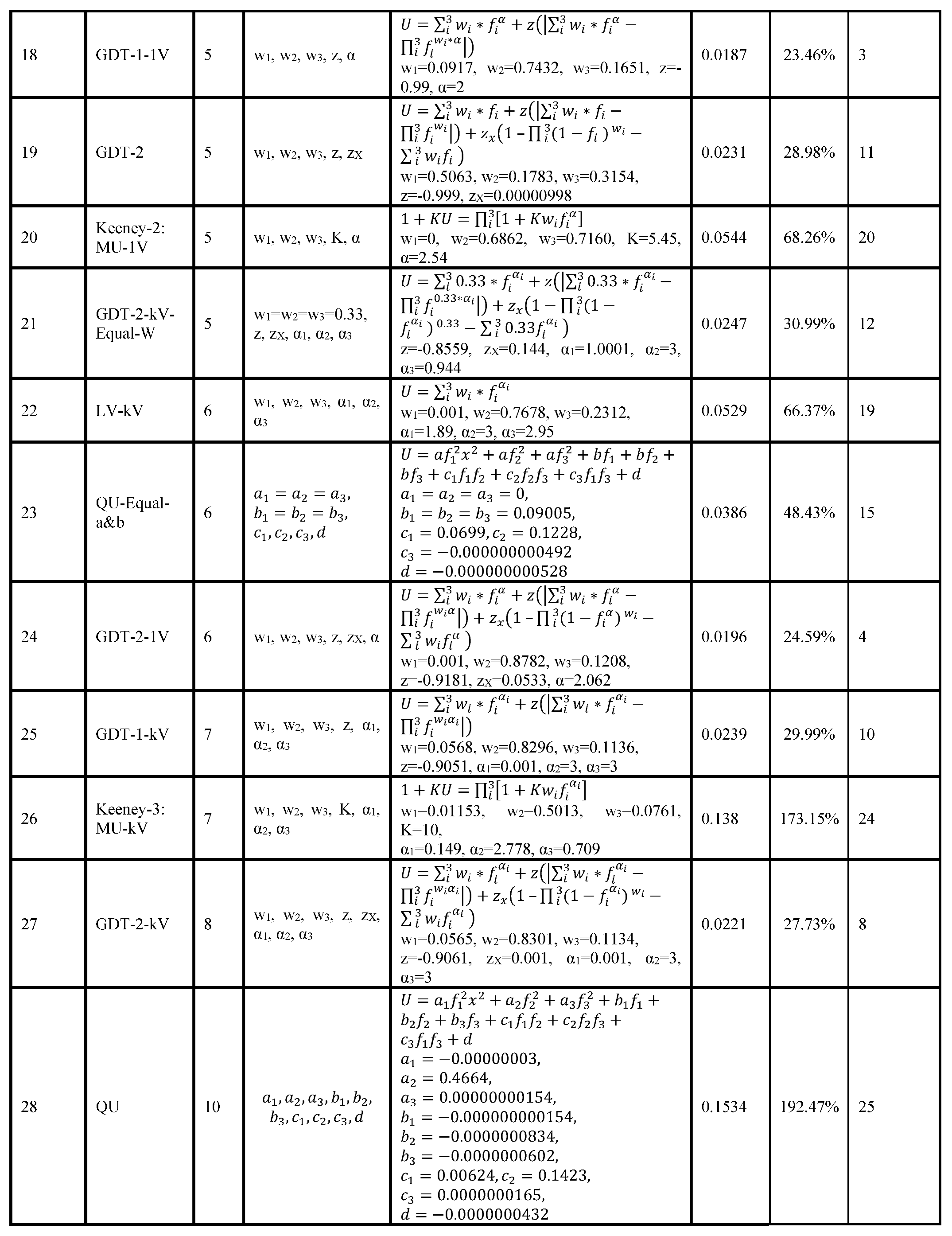
Table 10.
Example to show the differences between SD and GD when using dispersions.
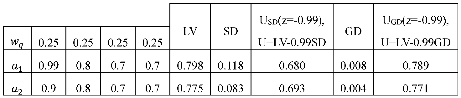
Table 11.
Rating of 13 Locations by Equal weights and z = -0.99.
Table 12.
Comparison of Aggregate ten DMs with varying z = 0, -0.5, and -0.99 values for five conflicting regions.
Table 12.
Comparison of Aggregate ten DMs with varying z = 0, -0.5, and -0.99 values for five conflicting regions.
| 2 | |
| 3 | To screen and clean up MCDM problem, one can first find the correlations of each pair of criteria and remove criteria that have high correlations with other criteria because they are essentially redundant. Also, one can identify criteria that have exceptionally low importance in MCDM models and discard them. For example, discard criteria whose wi (weight of importance) are less than a threshold (e.g., 0.05) in both LV and GDT-2 models. |
| 4 | In terms of communications with the DM, we can ask the DM to assess the utility values of a diverse sample of MCDM alternatives using a rating of 0.01 to 0.99 where 0.01 is the rating of the worst (hypothetical) alternative in which all fi=0.01; and 0.99 is the rating of the best (hypothetical) alternative in which all fi=0.99. Then use 70% of these alternatives to assess the utility function and use the remaining 30% to validate the model. Note that the no. of sample of alternatives should be substantially greater than (e.g., at least 1.5 times) the no. of parameters of the model. One reason for using is at least 1.5 data point is based on sample vs. out-of-sample analysis because (100%/70%) =1.43 rounds up to 1.5. For example, suppose k=3, then to test model XII in Table 4 which has ((2∗3)+2)=8 parameters, we need at least (8)∗(1.5)= 12 alternatives where we can use 70% or 0.7∗12=8.4 or 9 alternatives to assess the eight parameters of model XII and use the remaining (out-of-sample) 12-9=3 alternatives to validate the model and to examine if the DM agrees with the model assessment of the ratings of these three alternatives. We will show the details of above steps in the remainder of this paper. In this paper, we consider at least five randomly selected sample vs. the remaining out-of-sample alternatives. |
| 5 | We collected the ranking for purpose of helping DMs to be consistent, but we did use only ratings. |
| 6 | The meaning of this solution is that the utility function, U, is concave in vi = for all i, where is concave, is convex, is concave (because α<1 is concave and α>1 is convex) |
| 7 | It is, however, possible to give more value to extreme DMs by using a convex GDT-2 by setting z=0, or using a mixed concave and convex model in GDT-2 where both z and zX are used. |
Disclaimer/Publisher’s Note: The statements, opinions and data contained in all publications are solely those of the individual author(s) and contributor(s) and not of MDPI and/or the editor(s). MDPI and/or the editor(s) disclaim responsibility for any injury to people or property resulting from any ideas, methods, instructions or products referred to in the content. |
© 2024 by the authors. Licensee MDPI, Basel, Switzerland. This article is an open access article distributed under the terms and conditions of the Creative Commons Attribution (CC BY) license (http://creativecommons.org/licenses/by/4.0/).
Copyright: This open access article is published under a Creative Commons CC BY 4.0 license, which permit the free download, distribution, and reuse, provided that the author and preprint are cited in any reuse.


