
Submitted:
20 November 2024
Posted:
20 November 2024
You are already at the latest version
Abstract
We introduce the Hill-Wheeler equation as a quantum mechanical distribution function for nuclear fission, replacing the conventional Fermi-Dirac distribution function of the Fermi gas model. Our model treats fission fragments as harmonic oscillators without adjustable parameters. Through calculations using experimental data on nuclear fission product charge distributions, we found that the effective fission distance is proportional to the product of fragment charge numbers, and the compound nucleus possesses different effective fission barrier corrections for each constituent element. Comparing calculated effective nuclear fission barrier corrections with neutron separation energies showed good agreement with experimental nuclear fission cross-sections, demonstrating our model’s accuracy in describing nuclear fission characteristics.
Keywords:
Nuclear fission
; Statistical model
; Hill-Wheeler equation
; Quantum mechanical distribution function
; Distribution function
; Fission yield
; Scission distance
; Selective channel scission model
; Effective fission barrier correction
; Nuclear deformation
; Fission cross-section
1. Introduction
More than 80 years have passed since nuclear fission was discovered by Hahn and Strassmann in late 1938, yet its detailed mechanism remains not fully understood. Indeed, even the mass and charge distributions of fission products, which have been of interest since the discovery of nuclear fission, are still difficult to calculate theoretically. The mass distributions of commonly known nuclei such as and are not yet completely understood. Recent advances in computational capabilities and theoretical frameworks have significantly improved our understanding of fission mechanisms. Current research primarily focuses on four approaches:
Nevertheless, several fundamental issues remain unresolved, including the role of shell effects in determining fragment distributions, the mechanism of energy dissipation during the fission process, and the origin of mass asymmetry.
Various phenomenological models have been proposed to explain mass and energy distributions in nuclear fission:
In addition to these models, dynamical approaches have played crucial roles in deepening our understanding of nuclear fission. Specifically:
- Statistical decay theory using the Hauser-Feshbach formalism [14]
The model chosen was the selective channel scission (SCS) model, which was developed to theoretically calculate the mass and charge distributions of fission products. This model was proposed by Takahashi and Ota in 2001, and it is capable of calculating the yield by treating nuclear fission in terms of fission channels and finding the value of the fission barrier, Efi, for each possible channel [15,16,17,18,19,20].
The SCS model uses the following Hill-Wheeler equation [19,20]:
and determines the conditions for calculating the fission yield in the part of this equation, where , (fission barrier) and (effective fission barrier correction) are arranged as follows:
This can be used to calculate the transmittance:
which is derived to find the fission yield. The theoretical value of the mass number distribution of the fission product obtained by calculation was compared with experimental data, which showed that the calculation model using Eq. (3) was effective.
In this study, for the treatment of Hill-Wheeler Equation (1) with the SCS model,
- The Hill-Wheeler equation was used instead of the Fermi-Dirac distribution function used in statistical mechanics as the quantum mechanical statistical mechanics nuclear fission distribution function, and
- The two fragments produced during nuclear fission were considered harmonic oscillators
to derive an equation (statistical model of nuclear fission) that differed from Eq. (3).
Calculations were also conducted using experimental data on the charge distribution of the fission product yield. The details will be explained later, but the results obtained from this calculation are as follows.
- The effective scission distance at the moment that a nucleus splits into two fission fragments was obtained.
- The effective fission barrier correction was obtained by setting it as an unknown quantity and solving the simultaneous equations for all the patterns in which the nucleus splits into two fission fragments.
- The obtained maximum effective fission barrier correction was compared with the neutron separation energy, which showed that the values almost exactly matched the frequency of nuclear fission expected from the nuclear fission cross-section.
2. Calculation Using Statistical Model of Nuclear Fission with Hill-Wheeler Equation
The calculation conditions, calculation results, and calculation equation are shown here.
2.1. Calculation Conditions
The experimental data, target nucleus, etc., used for the calculations were as follows.
- JENDL-5 data [22] were used as the experimental data on the charge distribution for the fission product yield.
- Table 1 lists the eight types of target nuclei used in the calculations along with the calculation conditions.
It should be noted here that the calculation of this statistical model involved only the experimental data on the charge distribution of the fission product yield, neutron separation energy, neutron kinetic energy, and average number of generated neutrons, and that no adjustment parameters were set.
2.2. Calculation Results
The calculation results for the eight types of target nuclei are shown. The derivation of these results will be explained later, but the results are first presented in order to provide an overview.
-
Effective scission distance for each fission fragment: Figure 1, Figure 2 and Figure 3 show the obtained values.It can be seen from these calculation results that the effective scission distance was proportional to the product of the two fragments. In other words, the effective scission distance, (unit: fm), between fission fragments was the product of the charge numbers, Z, of the fission fragments and the atomic number - Z ⇒product of two fission fragments⇒ proportional to Z× (atomic number - Z) = Z × atomic number -.As shown in Figure 1, Figure 2 and Figure 3, the product of the charge numbers of the two fragments is larger toward the center. Thus, effective scission distance becomes larger. This is a reasonable and acceptable result.Figure 1. Scission distances of , , and as a function of fragment charge number. The calculated values demonstrate that the effective scission distance increases proportionally with the product of fragment charge numbers, reaching its maximum value near the center of the charge distribution.Figure 1. Scission distances of , , and as a function of fragment charge number. The calculated values demonstrate that the effective scission distance increases proportionally with the product of fragment charge numbers, reaching its maximum value near the center of the charge distribution.
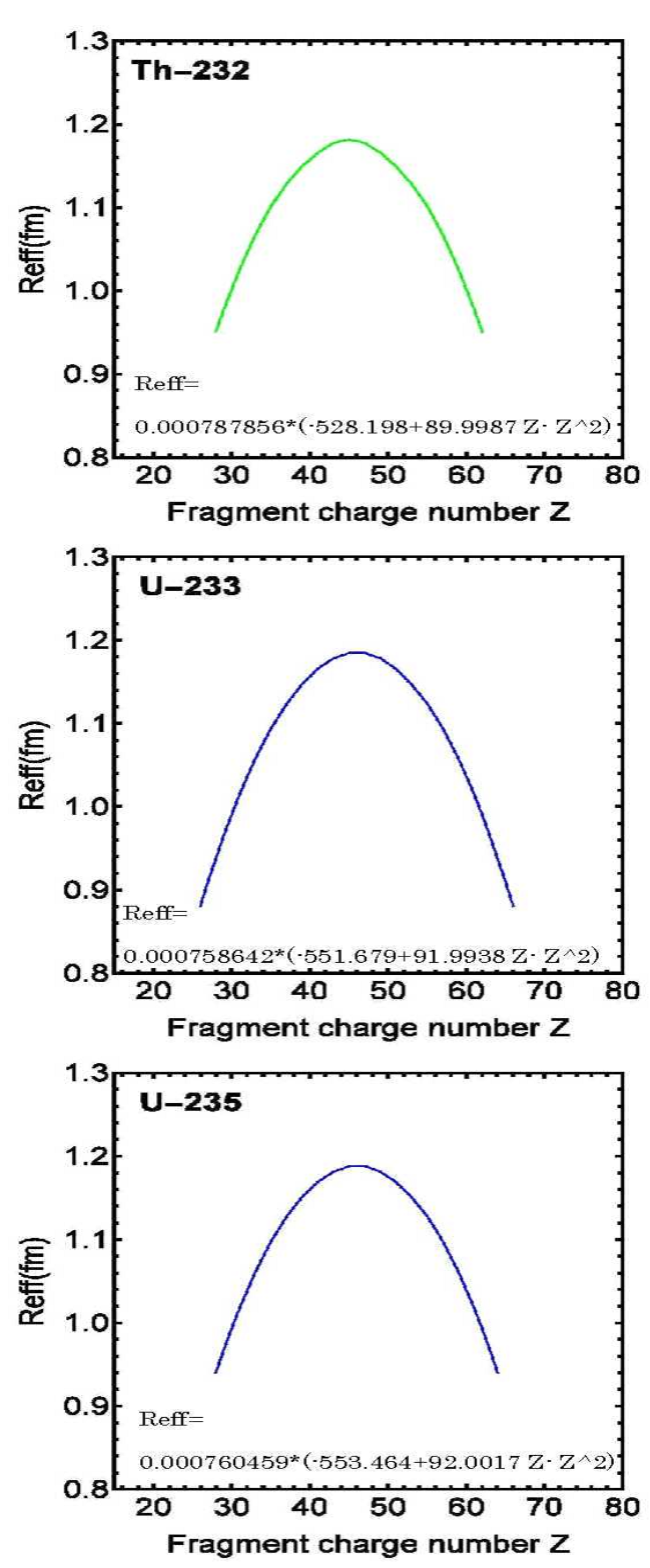 Figure 2. Scission distances of , , and as a function of fragment charge number. The relationship between fragment charge numbers and effective scission distance follows the same trend as observed in Figure 1, showing systematic behavior across different nuclei.Figure 2. Scission distances of , , and as a function of fragment charge number. The relationship between fragment charge numbers and effective scission distance follows the same trend as observed in Figure 1, showing systematic behavior across different nuclei.
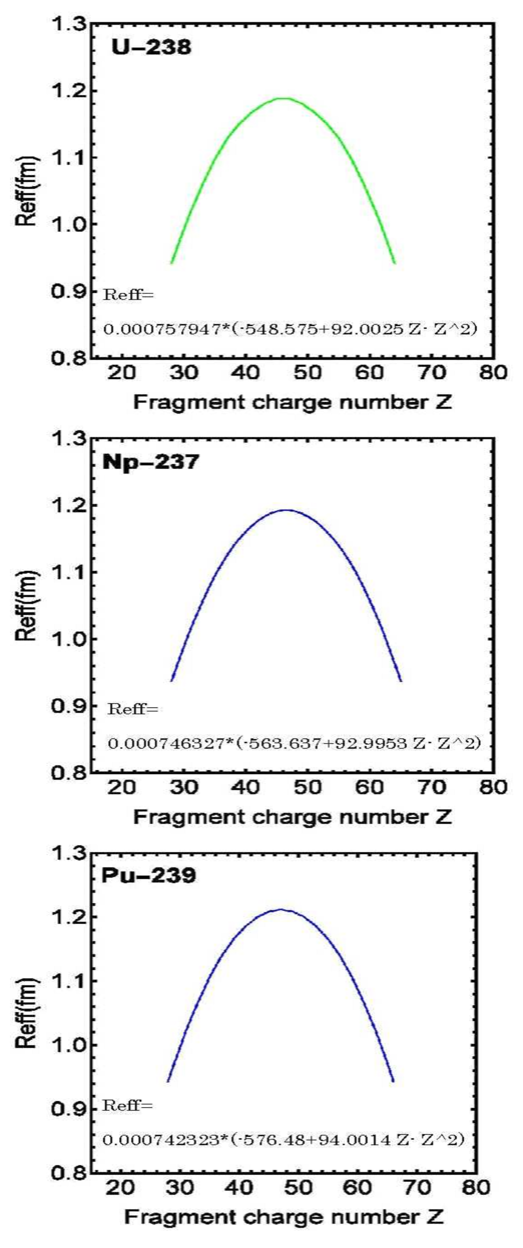 Figure 3. Scission distances of and as a function of fragment charge number. The calculated values confirm the systematic relationship between fragment charge numbers and effective scission distance observed in heavier plutonium isotopes.Figure 3. Scission distances of and as a function of fragment charge number. The calculated values confirm the systematic relationship between fragment charge numbers and effective scission distance observed in heavier plutonium isotopes.
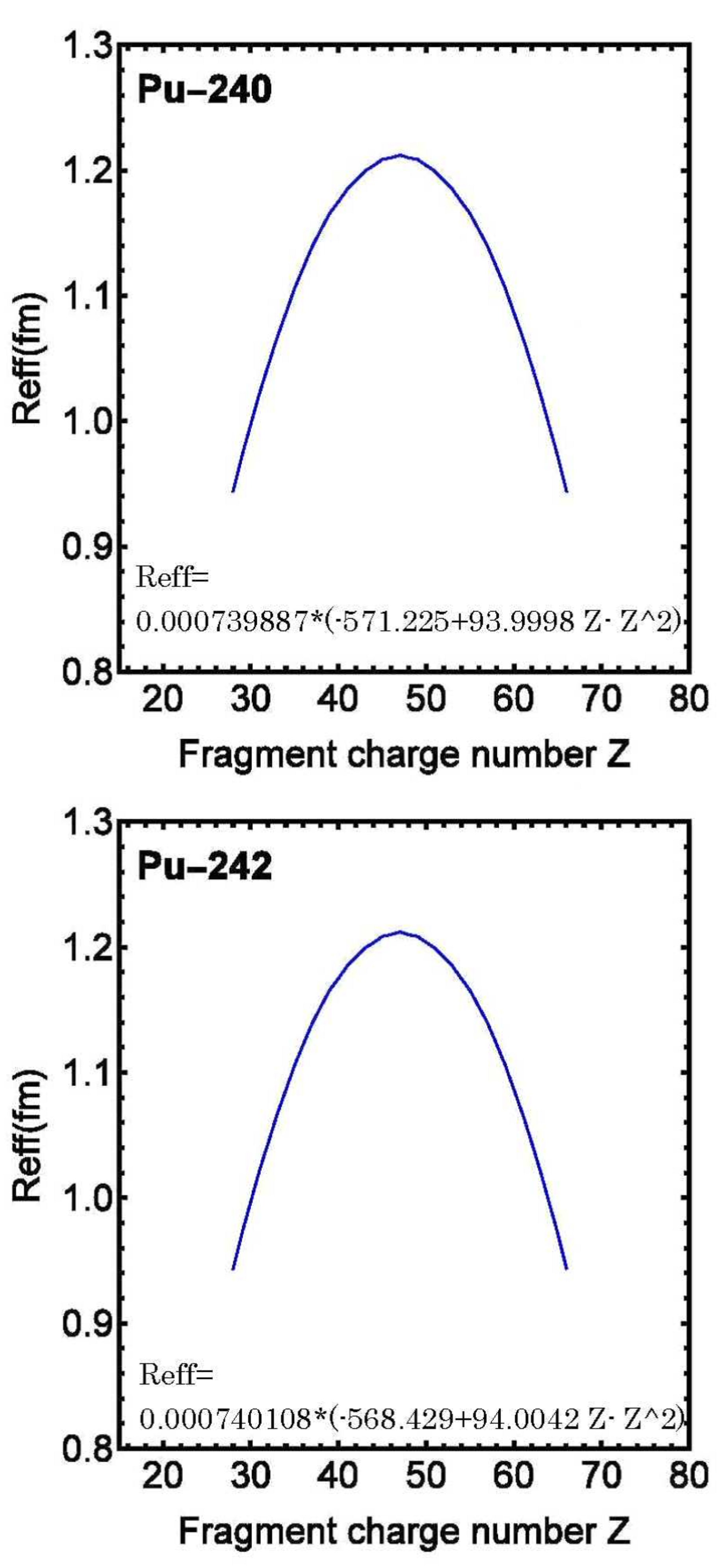
-
Figure 4, Figure 5 and Figure 6 show comparisons between experimental charge distributions and theoretical values calculated with zero effective fission barrier correction (ground state).Figure 4. Charge distribution (experimental curve) and theoretical values with zero effective fission barrier correction (ground state) of .Figure 4. Charge distribution (experimental curve) and theoretical values with zero effective fission barrier correction (ground state) of .
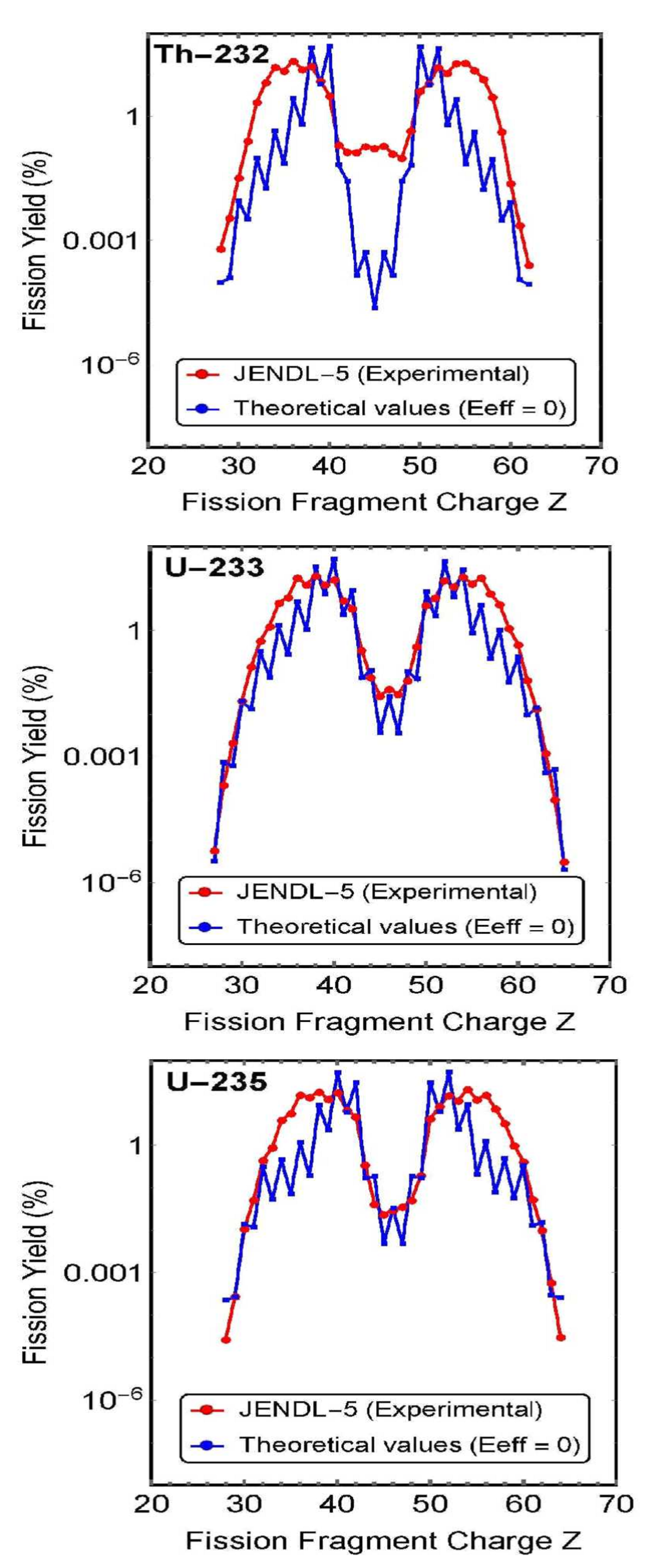 Figure 5. Charge distribution (experimental curve) and theoretical values with zero effective fission barrier correction (ground state) of .Figure 5. Charge distribution (experimental curve) and theoretical values with zero effective fission barrier correction (ground state) of .
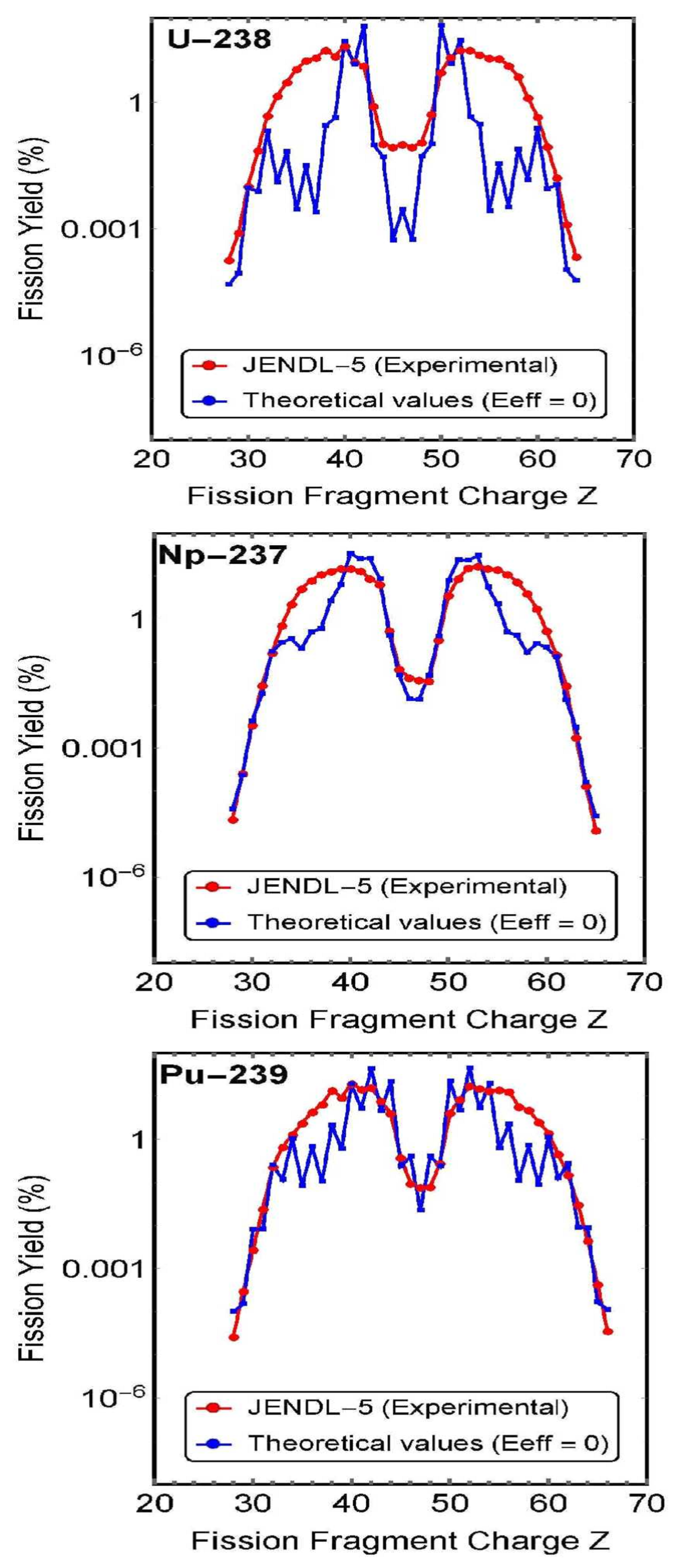 Figure 6. Charge distribution (experimental curve) and theoretical values with zero effective fission barrier correction (ground state) of .Figure 6. Charge distribution (experimental curve) and theoretical values with zero effective fission barrier correction (ground state) of .
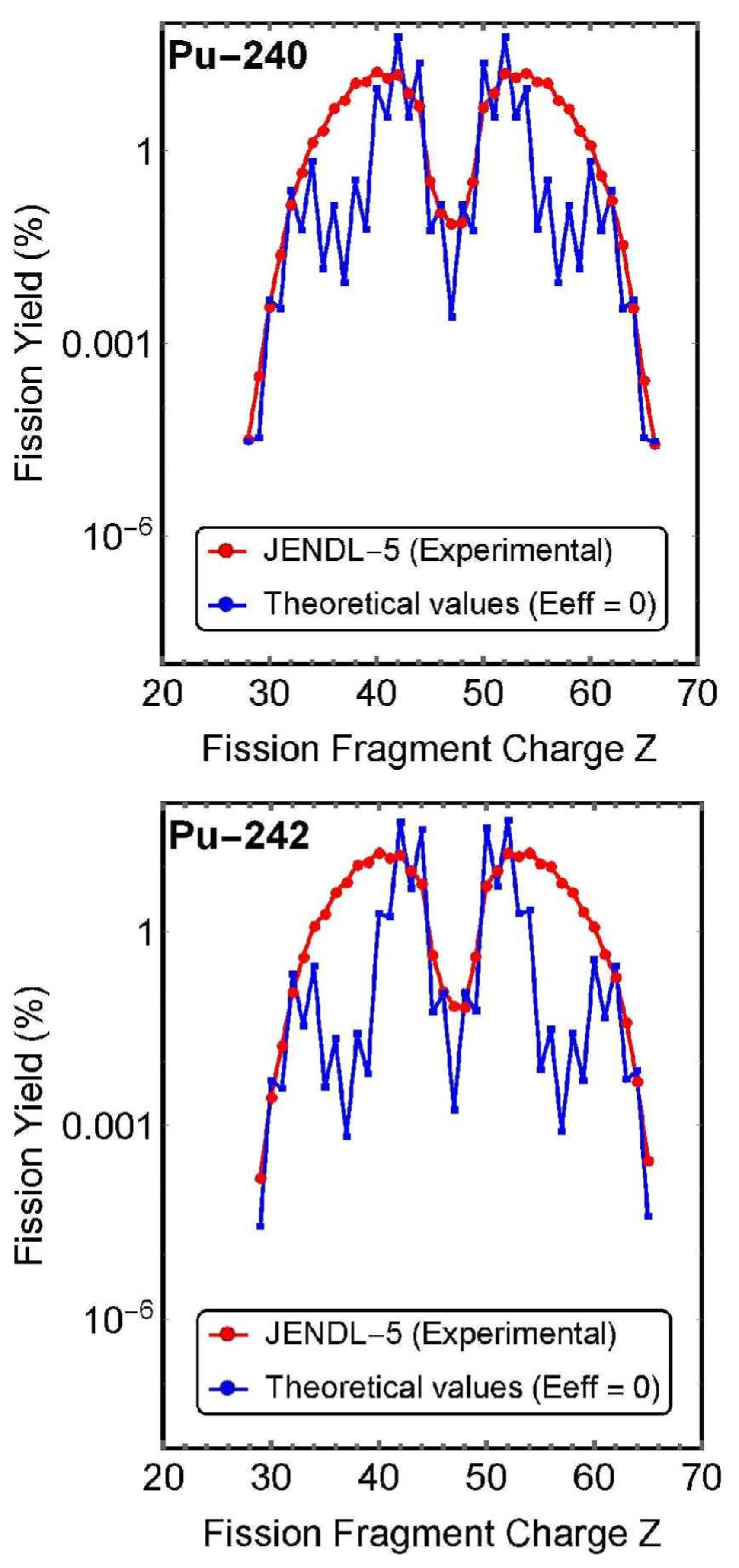 These figures show that the charge distribution curve is almost reproduced even when the effective fission barrier correction is zero (ground state).This reveals that most of the energy required for nuclear fission is the self-energy possessed by the nucleus (Coulomb force between two fragments), and that the energy required for fission is small compared to the self-energy.
 -
Figure 7, Figure 8 and Figure 9 show the obtained values for the effective fission barrier correction of each fission fragment of the nuclei.These figures show that the effective fission barrier correction values possessed by the nuclei were not uniform, but differed for each element of the fission fragments (the charges possessed by the fission fragments). The details of these calculation results will be discussed later.
2.3. Calculation Equation
2.3.1. Reason for Considering Hill-Wheeler Equation as Quantum Mechanical Nuclear Fission Distribution Function
The charge and mass number distributions of the fission products produced by nuclear fission have the same yield curves regardless of when the experiment is conducted. This signifies that nuclear fission occurs regularly according to the mathematical laws of physics. These should be physical laws that follow statistical mechanics (i.e., distribution functions). This conceptualization is verified in Appendix 1: Neutron spectrum ∝ state density x Fermi-Dirac distribution function.
Below, we explain why we chose the Hill-Wheeler equation as the distribution function during nuclear fission. First, we show the three types of distribution functions ((4), (5), and (6)) used in statistical mechanics. Gases and liquids composed of atoms and molecules that move according to classical mechanics follow the Maxwell-Boltzmann distribution:
Additionally, bosons such as photons, phonons, and Cooper pairs, which are responsible for the current in superconductors, follow the Bose-Einstein distribution function:
Finally, the behaviors of fermions such as protons and neutrons, in addition to electrons, are determined by the Fermi-Dirac distribution function:
Particles are distributed regularly according to these laws.
When statistical mechanics is applied to atomic nuclei, the Fermi gas model is used as the basis, and Eq. (6) is used as the distribution function. In this model, the phenomena that could be explained theoretically are limited to only one aspect for which there are experimental data, and the application scope is fixed.
Therefore, theoretical calculations were conducted using the transmittance equation derived by D.L. Hill and J.A. Wheeler assuming a harmonic oscillator, that is, the Hill-Wheeler Equation (7):
rather than the Fermi-Dirac distribution function.
This was done because Eq. (7) has the same form as the distribution function in Eq. (6), and although they have different designations (distribution function and transmittance equation), both are equations that calculate the existence probability based on the energy and ultimately involve the same calculation.
A comparison of Eqs. (6) and (7) shows that the value corresponding to ,k (Boltzmann constant) is ℏ (Planck constant), and both are constants. Furthermore, the value corresponding to t is , and both quantities increase with the energy. The two equations are different in appearance, but they are thought to be the same equations in content. In other words, this can be viewed as an equation where temperature energy is replaced by quantum mechanical value . Stated more boldly, the Hill-Wheeler Equation (7) can be viewed as a distribution function that is a further quantum mechanical basis of the Fermi–Dirac distribution function (6).
This is true for the following reasons.
- Temperature energy is a quantity that does not exist in a single atomic nucleus or molecule. It can be argued that this is why this is used in statistical mechanics, where a massive number of atoms and molecules exist. However, there should be no problem even if there is a more basic distribution function in which kt in the Fermi-Dirac distribution function (6), which is applicable even when there is only one atom or molecule, is replaced by .
- Additionally,if an equation that is simpler than Eq. (6) is considered from a quantum mechanical perspective, it is difficult to believe that equations other than (7) exist.
However, the above is an assumption without proof. The reality is unknown without actually attempting a calculation. In this study, an actual calculation was conducted to show that the above is correct.
As an aside, if the behavior of fermions follows Eq. (7), then the distribution function of the advanced quantum mechanical version of the Bose-Einstein distribution function that the boson follows is thought to be
Based on these analogies, and assuming that Eq. (7) corresponds to the distribution function during nuclear fission, the calculation equation was derived as follows. Whether this assumption is correct is discussed later by looking at the calculation results.
2.3.2. Derivation of Statistical Model of Nuclear Fission
Here, the equation for the statistical model of nuclear fission is derived from the Hill-Wheeler Equation (7), which is thought to be the equation for the distribution function of the advanced quantum mechanical version.
As mentioned above, the points derived assuming that Eq. (7) is a harmonic oscillator should be satisfied. Therefore, it is assumed that the atomic nucleus is a harmonic oscillator with fission fragments FP1 and FP2 connected by an ideal spring, as shown in Figure 10. (Because charge distribution experimental data are considered, charge numbers Z1 and Z2 are used instead of the mass as the harmonic oscillator of the fission fragments.)
The Hill-Wheeler equation can be rewritten as follows:
This equation was derived by Hill and Wheeler from the Schrödinger equation assuming a harmonic oscillator [21,23,24,25] , where the potential of the harmonic oscillator is found as follows:
The denominator, , is the angular frequency of the harmonic oscillator, and if of the harmonic oscillator is the force constant, then it is found as follows:
The reduced mass, , uses charge numbers Z1 and Z2 as shown in Figure 10. Thus, it is found as follows:
Then, Eq. (9) can be rewritten as follows:
where is the product of charge numbers Z1 and Z2, as shown in Eq. (12), and draws a parabola. Thus, when the maximum value is set as and the equation is written as follows:
then
Here, Eq. (15) is compared with the form of the Fermi-Dirac distribution function followed by fermions:
The value corresponding to in the Fermi-Dirac distribution function (16) is in Eq. (15). The neutron energy that is incident on the target nucleus is thought to correspond to temperature energy . This is because, in the same way that the distribution state inside a container (e.g., solid, semiconductor) changes depending on the change in temperature energy kt for the Fermi–Dirac distribution function (16), the distribution state inside the container (atomic nucleus) also changes depending on the incident neutron energy, even in the case of the distribution function Equation (15). Therefore, if neutron separation energy and neutron kinetic energy, then the following replacement can be performed:
This results in
where is found using an equation similar to Eq. (2) of the SCS model, as the difference between (fission barrier) and (effective fission barrier correction):
In the nuclear fission calculations discussed here, becomes the effective parameter, and both and change for each element that constitutes the nuclear material (later changed from to ). The calculation of will be explained in the following section, and changes in will be discussed later.
Based on these, the final equation for the statistical model of nuclear fission using the Hill-Wheeler equation becomes
As previously mentioned, Eq. (20) of this statistical model uses only the experimental data on the charge distribution of the fission product yield, neutron separation energy, kinetic energy of the incident neutrons, and average number of generated neutrons, with no adjustment parameters needed.
2.3.3. Calculation Process for Deriving Charge Distribution from Statistical Model of Nuclear Fission
Here, we use Eq. (20) of the statistical model of nuclear fission derived from the Hill-Wheeler equation to show the calculation process up to finding the charge distribution.
Various numerical calculations have been attempted in the vicinity of the potential peak shown in Figure 11, but there is no definitive method. It is currently thought that the potential may form multiple peaks as a result of the shell effect, but in the case discussed here, the effective fission barrier correction has a different value for each fission fragment, which results in a structure that forms fission isomers. However, the assumption during calculations is a single peak structure. This assumption is shown to be correct from later calculation results because the fission energy when calculating the charge distribution is mostly due to the Coulomb force between the two fragments, and the influence of the nuclear force is extremely small compared to this energy. Thus, there is no problem with the assumption of a single peak structure.
Repeating the explanation, strictly speaking, the potential forms multiple peaks, but most of these are due to the Coulomb force between the two fragments. Thus, considering a single peak structure does not present a problem. In other words, the result is that there are small and jagged undulations in a single peak.
As shown in Figure 11, if the two fission fragments after fission are far enough apart, then the value becomes equivalent to the Coulomb potential. Therefore, it is assumed that fission occurs at the internuclear distance when the Coulomb potential between bare fragments corresponds to a channel-dependent fission barrier. This internuclear distance is called the effective scission distance, , which is defined as follows after introducing scission-related parameters and :
where and are the fragment charge numbers after scission. Here, and , which are parameters associated with the scission, are introduced because it is thought that the shape of the nucleus during fission stretches in proportion to the size of fission fragment charge numbers Z1 and Z2 when the shape is spherical, as shown in Figure 11, as a result of going through the deformation process leading to scission. Therefore, the inter-fragment distance, which considers this stretching, is a value that takes into account the product of the fragment charge numbers (), along with parameters and . The values of parameters and can be automatically calculated from experimental data. Therefore, there is no need to determine them artificially.
The value of the channel-dependent fission barrier, , is found by subtracting the Q value for each fission reaction from the value of the inter-fragment Coulomb potential (effective Coulomb energy) at the effective scission distance, :
where Coulomb potential on the right side of this equation is found as follows:
These values are substituted into Eq. (20) of the statistical model of nuclear fission for each fission reaction, and finally, as shown by
the total for each fission reaction is obtained, along with the charge distribution yield of each fission product.
is the total of all the isotopes (subscript j) of the fission fragments that may be generated during nuclear fission. For example, in the case of , which has atomic number i = 56, all the values from to that can be considered to exist as fission products are added together.
2.3.4. Specific Calculation
The calculation process when using the statistical model of nuclear fission to determine the charge distribution of the fission yield was described in the previous section. However, in this study, experimental data for the charge distribution were used in the calculation (i.e., calculation conditions). Then, as shown in the calculation results in §2.2. , the following three calculations were conducted.
-
Calculation of effective scission distance for each pair of fission fragmentsIn in Eq. (19), effective fission barrier correction , and effective scission distance in Eq. (21), which is included in Eq. (20), was obtained as an unknown quantity. As shown in Figure 1, Figure 2 and Figure 3, the result was that the effective scission distance was proportional to charge number Z of the two fission fragments. In other words, the distance was proportional to (atomic number-Z)= atomic number-.
-
Calculation of charge distribution when effective fission barrier correction is zero (ground state)The theoretical value of the charge distribution was calculated using the value of Eq. (21) obtained in (1) above, along with Eq. (20) with effective fission barrier correction (ground state) in in Eq. (19). Figure 4, Figure 5 and Figure 6 show diagrams comparing the experimental charge distributions and theoretical values calculated with . As can be seen from the figures, even when effective fission barrier correction , the theoretical values were in good agreement with the experimental charge distributions.
-
Calculation of effective fission barrier correction for each fission fragmentFirst, in Eq. (19) was changed to . In other words, it was assumed that different effective fission barrier corrections, , existed depending on the channel. Then, using effective scission distance obtained from Eq. (21) and considering to be an unknown quantity, simultaneous equations for all patterns in which a compound nucleus became two fission fragments were solved to obtain the charge distribution of the fission yield, thereby obtaining the effective fission barrier correction. As a result, as shown in Figure 7, Figure 8 and Figure 9, effective fission barrier corrections, , with different values for each element (fission fragment) constituting the compound nucleus were obtained.
3. Calculation Results and Discussion
Here, the following points obtained from the calculations are considered.
- (1)
- (2)
- As shown in Figure 4, Figure 5 and Figure 6, when the charge distribution was calculated with the effective fission barrier correction set to zero, a theoretical value for the charge distribution close to the experimental value was obtained even at zero value. The meaning of this result is discussed.
- (3)
- As shown in Figure 7, Figure 8 and Figure 9, the effective fission barrier correction had different values depending on the elements that constituted the nucleus (i.e., for each fragment). It is currently generally thought that the entire compound nucleus has a uniform effective fission barrier correction when a neutron is incident on a target nucleus. Whether the effective fission barrier correction of a compound nucleus is uniform, or whether it differs for each element (fission fragment), is discussed.
- (4)
3.1. Discussion of (1)
The calculation results shown in Figure 1, Figure 2 and Figure 3 indicate that the Coulomb repulsion and effective scission distance reach their maximum values when the product of fission fragment charge numbers Z1 and Z2 (atomic number - Z1) is the largest.This value was derived by calculating effective scission distance as an unknown quantity, which was in agreement with the intuitive understanding of nuclear fission.It is difficult to think that the distance at which nuclear fission occurs is independent of charge numbers Z1 and Z2. It is currently not possible to experimentally confirm how nuclear fission occurs, but as shown in Figure 1, Figure 2 and Figure 3, the most natural conclusion is that fission is proportional to the product of fission fragment charge numbers Z1 and Z2, which matches our intuition on the subject.
Additionally, the calculation results shown in Figure 1, Figure 2 and Figure 3 indicate that effective scission distance is approximately 1.0-1.2 fm. The nuclear force potential value cannot be directly obtained by experiment, but if this is calculated using the Woods-Saxon model or QCD lattice theory, then this indicates that the calculation result of the potential value sharply weakens when the radius has a value of approximately 1 fm or more, as shown in Figure 12 [26].
This result also does not rule out the outcome that effective scission distance is approximately 1.0-1.2 fm. It is thought that this indicates that the nuclear force weakens at approximately 1.2 fm, the inter-fragment Coulomb repulsion prevails, and nuclear fission occurs.
As mentioned above, results were obtained for the eight calculated nuclide types where fission was proportional to the product of fission fragment charge numbers Z1 and Z2, and effective scission distance was approximately 1.0-1.2 fm. It is difficult to conceive that such a simple result could be produced by chance. Therefore, it is thought that the statistical model of nuclear fission (20), which was created based on the assumption that the Hill-Wheeler Equation (7) corresponds to the nuclear fission distribution function, is one of the proofs of its effectiveness.
3.2. Discussion of (2)
The calculation results shown in Figure 4, Figure 5 and Figure 6 indicate that when the charge distribution is calculated based on the assumption that the effective fission barrier correction is zero, then a charge distribution (theoretical value) that is almost equivalent to the experimental value is obtained even with zero correction value (i.e., the ground state where no neutrons are incident).
This calculation result shows that, even in the ground state, the nucleus itself has most of the energy to cause nuclear fission as self-energy (Coulomb energy). Therefore, if a small amount of missing energy (effective fission barrier correction) is added to the theoretical curve of the charge distribution at zero correction value (ground state) shown in Figure 4, Figure 5 and Figure 6, then the theoretical curve will be in agreement with the experimental value of the charge distribution.
3.3. Discussion of (3)
The effective fission barrier corrections shown in Figure 7, Figure 8 and Figure 9 correspond to the above-mentioned small amount of missing energy. When this correction value is added to the theoretical curve of the charge distribution at zero correction value (ground state) shown in Figure 4, Figure 5 and Figure 6, the theoretical curve of the charge distribution matches the experimental value.
A concern here is that, as shown in Figure 7, Figure 8 and Figure 9, the effective fission barrier correction of the compound nucleus has a different value for each element that constitutes the nucleus (i.e., fission fragment). It is currently thought that the entire nucleus has a uniform effective fission barrier correction when a neutron is incident on a target nucleus. Regarding this aspect, the author believes that the effective fission barrier correction of a nucleus has a different value for each element that constitutes the nucleus for the following reasons.
Take as an example. When a neutron is incident on this nucleus, a compound nucleus is formed. Currently, this compound nucleus is considered to have a "uniform effective fission barrier correction." This "uniform" aspect does not make sense. Indeed, if the nucleus were a perfect sphere, then it might have a uniform effective fission barrier correction. However, experiments have shown that is rugby ball-shaped. Then, it is generally correct to think that the correction state differs with the location of .
The rugby ball shape of means that the nuclear force of neutrons and protons differs depending on the location of . If the incident neutrons are taken in and the nuclear force differs depending on the location, then the possibility of a uniform and equivalent effective fission barrier correction of is low. It should be considered that the effective fission barrier correction of could differ with the location.
3.4. Discussion of (4)
Here, the calculation results shown in Figure 7, Figure 8 and Figure 9 are compared with the experimental results. Table 2 lists the nuclear reactions at which the effective fission barrier correction is maximized, along with their values. The value at which the effective fission barrier correction is at a maximum is thought to correspond to the critical energy.
Here, representative nuclides , and are extracted from Table 2, and the maximum values of the effective fission barrier corrections obtained by calculations (critical energy) are compared with the neutron separation energies. (The values were rounded off to one decimal place.)
- 1.
-
In the case of ,and if it is interpreted that nuclear fission is more likely to occur when the neutron separation energy exceeds the critical energy, then this is consistent with the experimental result of a nuclear fission cross-section of 585.1 b.
- 2.
-
In the case of ,and if it is interpreted that nuclear fission is less likely to occur when the neutron separation energy is less than the critical energy, then this is consistent with the experimental result of a nuclear fission cross-section of 16.8b.
- 3.
-
In the case of ,and if it is interpreted that nuclear fission is more likely to occur when the neutron separation energy exceeds the critical energy, then this is consistent with the experimental result of a nuclear fission cross-section of 747.4 b.
These results show that comparing the maximum value of the effective fission barrier correction (critical energy) and the neutron separation energy makes it possible to predict the frequency of nuclear fission to some extent. However, the effective fission barrier corrections shown in Figure 7, Figure 8 and Figure 9 are continuously distributed. Therefore, the frequency of nuclear fission needs to be evaluated by comparing the neutron separation energy with not only the maximum value of the correction but also with all of its continuous values.
As a result, Table 2 is only a guideline for predicting the frequency of nuclear fission, and it is necessary to evaluate the continuously distributed effective fission barrier correction by comparing it with the neutron separation energy. However, once again, it is thought that comparing the maximum value of the effective fission barrier correction with the neutron separation energy allows for a rough guideline for predicting the frequency of nuclear fission.
This result is also thought to be one of the proofs of the validity of the statistical model of nuclear fission (20), which was created by assuming that the Hill-Wheeler Equation (7) corresponds to the nuclear fission distribution function.
4. Conclusion
In this study, we used the Hill-Wheeler equation to create a statistical model of nuclear fission, and the following values were obtained based on the experimental data on the charge distribution of the fission product yield:
- Frequency of nuclear fission based on comparisons of the effective fission barrier correction and neutron separation energy (Table 2).
These were summarized in section 3: Calculation results and discussion.
There is room for improvement in the calculations for points 2. and 3., as explained below. First, for point 2., it is thought that a more accurate effective fission barrier correction could be obtained by calculating the number of emitted neutrons, which differs with the fission fragment. The reason for this is explained.
Finding the effective fission barrier correction requires finding fission barrier during the calculation (reprinted by substituting Eq. (23) into Eq. (22):
In this calculation, the average value, as listed in Table 1, is used as the number of neutrons emitted during nuclear fission. However, at a basic level, the number of generated neutrons takes a different value for each nuclear fission reaction.
Moreover, the number of neutrons generated in each nuclear reaction is presently unknown. Thus, accurate Q values cannot be determined. For example, in the case of , the number of generated neutrons is calculated as an average value of two neutrons for all reactions in order to obtain the Q value, as shown in the following:
However, in practice, the number of neutrons emitted in each case should be different, such as 3 or 1. Obtaining a more accurate nuclear fission barrier (critical energy) requires considering the actual number of neutrons released in each nuclear reaction rather than the average number.
This is thought to result in an accurate Eq. (25) as well as an even more accurate value for the effective fission barrier correction. However, it is difficult to experimentally determine an accurate number of emitted neutrons (generated neutron multiplicity), and research is currently being conducted on mass distributions using the Hauser–Feshbach statistical decay theory. However, work on the charge distribution is still in the research stage, and there were no experimental data. Therefore, the average value was used for calculations.
For point 3., Table 2 was created in order to predict the frequency of nuclear fission, and a comparison was made of the maximum value of the effective fission barrier correction, that is, the critical energy (calculated value), and the height between the points of neutron separation energy (i.e., a comparison of only two values). Furthermore, making more accurate frequency predictions requires a two-dimensional evaluation of a comparison of the continuously distributed effective fission barrier corrections shown in Figure 7, Figure 8 and Figure 9 with the neutron separation energies.
If this were compared to mountain climbing, this is not the same as just climbing a single mountain with a high altitude, but rather, a mountain with complicated ridges and smaller mountains scattered about, despite having a lower altitude, which would require more energy than the former. In this way, the accuracy when predicting the frequency of nuclear fission could be improved if it was possible to conduct a two-dimensional comparison and evaluation of the continuously distributed effective fission barrier correction and neutron separation energy.
Acknowledgments
We would like to express our sincere gratitude to many individuals who provided support and guidance throughout this research. In particular, we extend our heartfelt thanks to Claude and ChatGPT for providing extensive translation and editing support, as well as technical advice. Their collaboration enabled us to compile and present our research findings effectively. We would also like to express our deep appreciation to everyone who made significant contributions regarding the numerical values, research resources, and data analysis presented in this paper.
Appendix A. Prompt Neutron Spectrum ∝ State Density × Fermi-Dirac Distribution Function
Here, an explanation is provided for the fact that the energy spectrum of prompt neutrons is expressed by the state density × Fermi-Dirac distribution function, just like the spontaneously emitted light from semiconductors.
Appendix A.1. Spectrum of Spontaneously Emitted Light from Semiconductors
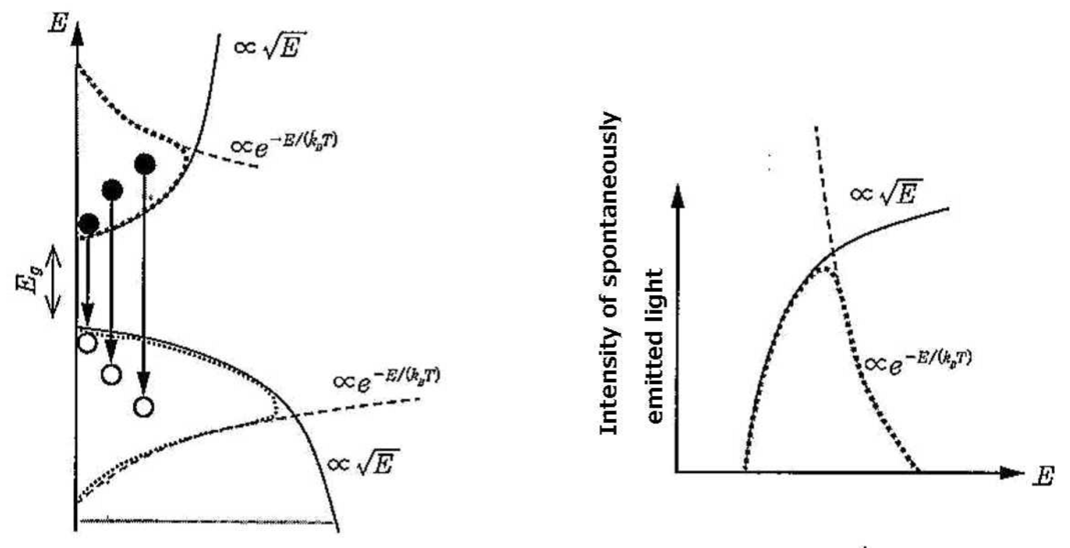
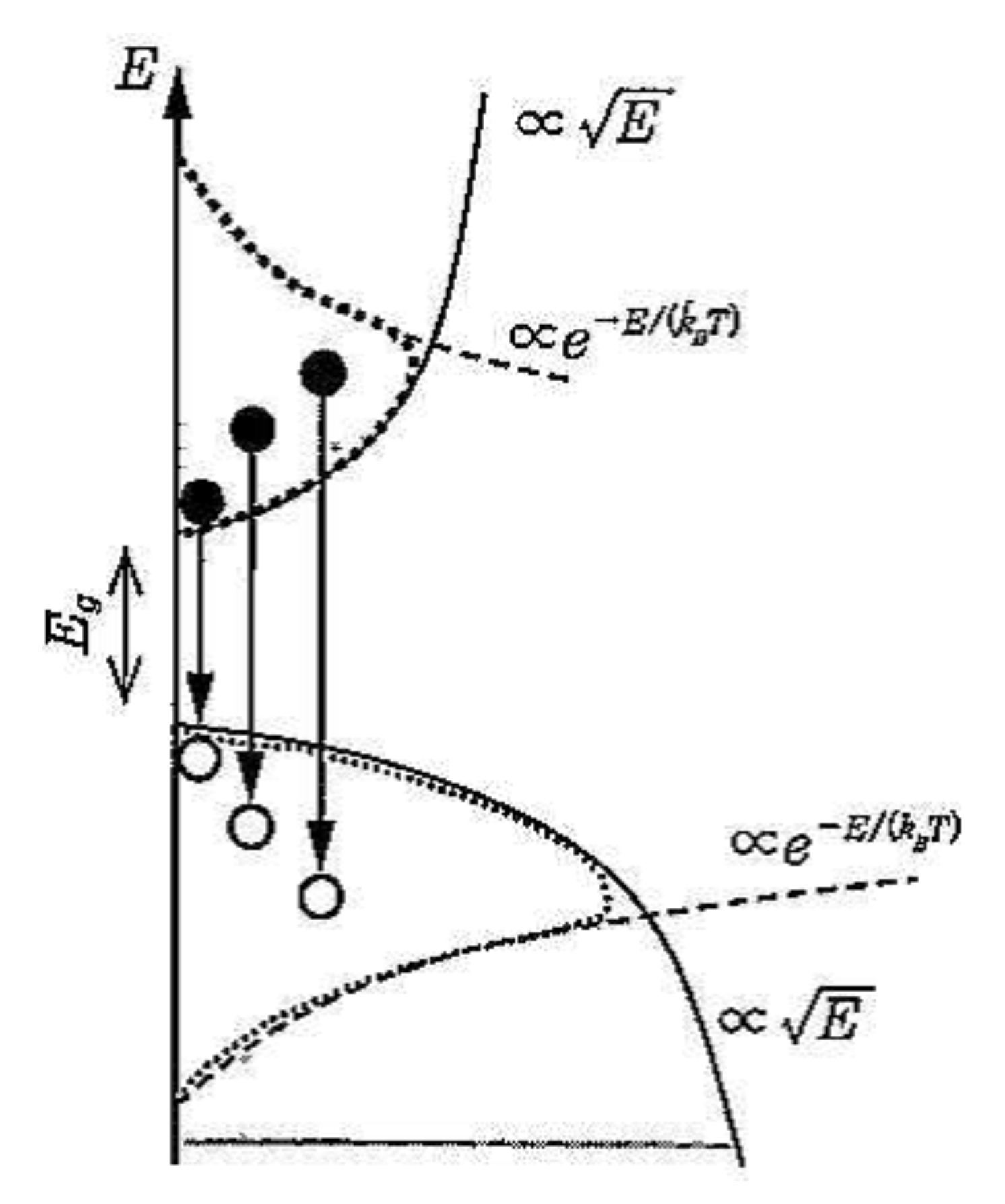
The spectral shape of the spontaneously emitted light from semiconductors can be expressed as shown in Figure 13.
These figures illustrate the relationship between prompt neutron energy spectra and the Fermi-Dirac distribution function:
This shape can be expressed using the following equation:
and it follows the energy distribution of the electron state density on the low energy side, with the Boltzmann distribution being reflected on the high energy side. In other words, in semiconductors, the electron and hole energies spread out according to the Fermi-Dirac distribution function.
Figure A1.
Conceptual diagram showing spontaneous emission spectra from semiconductors, provided as an analogous system [27].
Figure A1.
Conceptual diagram showing spontaneous emission spectra from semiconductors, provided as an analogous system [27].
Appendix A.2. Energy Spectrum of Prompt Neutrons
Figure 13 shows the spectrum of the prompt neutrons. As shown in the figure, this equation can be expressed as follows:
Figure A2.
Energy spectrum of prompt neutrons demonstrating the similarity to semiconductor emission patterns [28].
Figure A2.
Energy spectrum of prompt neutrons demonstrating the similarity to semiconductor emission patterns [28].
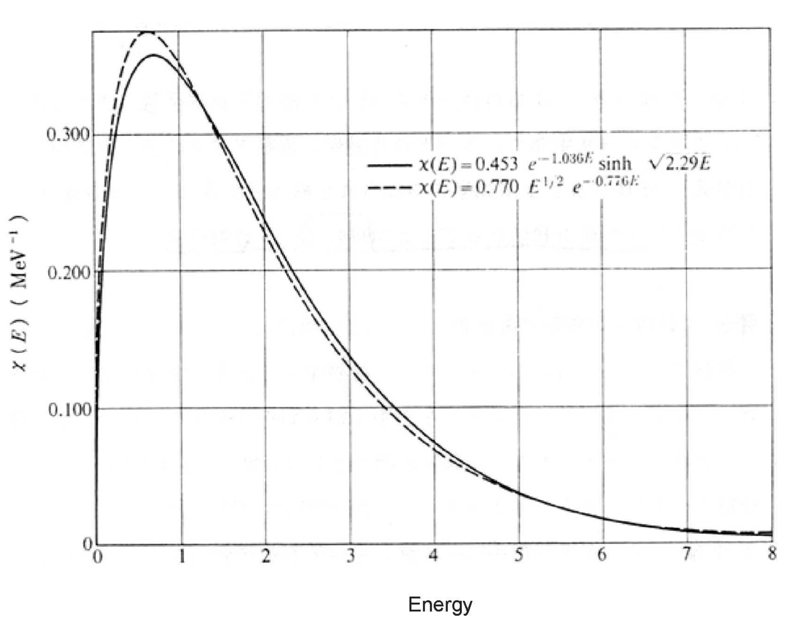
and it generally has the same form as Eq. (27) for the spontaneously emitted light from semiconductors (although the coefficients are different). The energy distribution of the neutron state density is reflected on the low energy side, and the Boltzmann distribution is reflected on the high energy side. In nuclear fission, as with semiconductors, the proton and neutron energies follow the Fermi–Dirac distribution function. Thus, theorizing should be done using the conceptual diagram of Figure 15 (figure of state density and Fermi-Dirac distribution function), which is used in semiconductor engineering, and this supports the general accuracy of the approach used here.
Figure A3.
Schematic representation of prompt neutron emission from nuclear fission, highlighting the role of state density and Fermi-Dirac distribution [27].
Figure A3.
Schematic representation of prompt neutron emission from nuclear fission, highlighting the role of state density and Fermi-Dirac distribution [27].
Appendix B. Attachment of MATHEMATICA Calculation Program
The Mathematica code and PDF files containing calculation results used in this study are available at the following links:
- MathematicaCode: MathematicaCode.zip
- Mathematica Calculation Results (PDF): MathematicaPDF.zip
Critical Computational Requirements: This study’s numerical calculations, which utilize the Hill-Wheeler equation, operate correctly only with Mathematica versions 9 through 11.2. Due to fundamental specification changes in the FindMinimum command implemented from version 11.3 onwards, it is absolutely impossible to perform these calculations correctly in any later versions. This is not a limitation of our methodology, but rather a direct consequence of the command specification changes. Therefore, any attempt to reproduce these calculations must use Mathematica versions 9-11.2. We particularly recommend version 11.2, which has been extensively used for verification in this study.
References
- Schunck N, Robledo LM. Microscopic theory of nuclear fission: a review. Rep. Prog. Phys. 2016 Nov;79:116301-116380. [CrossRef]
- Schunck N, Dobaczewski J, Sarich J, McDonnell JD, Nazarewicz W, Sheikh J, Staszczak A, Stoitsov M, Toivanen P, Yu Y. Solution of the Skyrme-HFB equations in the Cartesian deformed harmonic-oscillator basis. Comp. Phys. Comm. 2017 Jul;216:145-174.
- Regnier D, Dubray N, Schunck N, Verriere M. Fission fragment charge and mass distributions in 239Pu(n,f ) in the adiabatic nuclear energy density functional theory. Phys. Rev. C 2019 Feb;99:024611-024628.
- Zhao J, Lu BN, Nikšić T, Vretenar D. Time-dependent density functional theory with pairing dynamics of nucleons for fission and fusion reactions. Phys. Rev. C 2019 May;99:054613-054630.
- Pang LG, Wu K, Zhou X, Song T, Müller B, Qin G, Wang XN, Kim SY, Ma YG, Bentz W. Nuclear data applications of machine learning. Nature Reviews Physics 2021 Mar;3:311-323.
- Talou P, Kawano T, Stetcu I, Jaffke P, Lovell AE, Randrup J. Quantified uncertainties in fission observables: Current status and future needs. EPJ Web of Conferences 2019 Mar;211:04004-04012.
- Randrup J. Nuclear fission dynamics: collective aspects of fission fragment formation. Phys. Rev. C 2010 Dec;82:064905-064925.
- Ishizuka C, Usang MD, Ivanyuk FA, Maruhn JA, Nishio K, Chiba S. Four-dimensional Langevin approach to low-energy nuclear fission of 236U. Phys. Rev. C 2017 Dec;96:064616-064635.
- Brosa U, Grossmann S, Müller A. Nuclear scission. Phys. Rep. 1990 Dec;197:167-262.
- Wilkins BD, Steinberg EP, Chasman RR. Scission-point model of nuclear fission based on deformed-shell effects. Phys. Rev. C 1976 Nov;14:1832-1863. [CrossRef]
- Möller P, Madland DG, Sierk AJ, Iwamoto A. Nuclear fission modes and fragment mass asymmetries in a five-dimensional deformation space. Nature 2001 Feb;409:785-790. [CrossRef]
- Schmidt KH, Jurado B. Review on the progress in nuclear fission—experimental methods and theoretical descriptions. Rep. Prog. Phys. 2018 Oct;81:106301-106345. [CrossRef]
- Sierk AJ, Capote R, Kawano T, Schmidt KH, Talou P, Ward DE. Langevin studies of fission dynamics. Phys. Rev. C 2019 Jul;100:014610-014632.
- Okumura S, Kawano T, Jaffke P, Talou P, Chiba S. 235U(n,f) Independent fission product yield and isomeric ratio calculated with the statistical Hauser-Feshbach theory. J. Nucl. Sci. Tech. 2018 Sep;55:1009-1023.
- Takahashi A, Ohta M, Mizuno T. Production of stable isotopes by selective channel photofission of Pd. Jpn. J. Appl. Phys. 2001 Dec;40:7031-7039. [CrossRef]
- Ohta M, Matsunaka M, Takahashi A. Analysis of 235U fission by selective channel scission model. Jpn. J. Appl. Phys. 2001 Dec;40:7047-7053. [CrossRef]
- Ohta M, Takahashi A. Analysis of incident neutron energy dependence of fission product yields for 235U by the selective channel scission model. Jpn. J. Appl. Phys. 2003 Feb;42:645-652. [CrossRef]
- Ohta M, Nakamura S. Channel-dependent fission barriers of n+235U analyzed using selective channel scission model. Jpn. J. Appl. Phys. 2006 Aug;45:6431-6438.
- Ohta M, Nakamura S. Simple Estimation of Fission Yields with Selective Channel Scission Model. J. Nucl. Sci. Technol. 2007 Nov;44:1491-1499.
- Ohta M. Influence of deformation on Fission Yield in Selective Channel Scission Model. J. Nucl. Sci. Technol. 2009 Jan;46:6-11.
- Hill DL, Wheeler JA. Nuclear Constitution and the Interpretation of Fission Phenomena. Phys. Rev. 1953 Mar;89:1102-1145. [CrossRef]
- Iwamoto O, Iwamoto N, Kunieda S, Minato F, Nakayama S, Abe Y, Aoyama S, Daido R, Furutachi N, Fujimoto R, Fukahori T, Goko S, Harada H, Hashimoto S, Ichihara A, Igashira M, Ishibashi N, Katabuchi T, Katakura J, Kawano N, Kawano T, Kikuzawa N, Kitazawa H, Kohno T, Maekawa F, Murata T, Nakano M, Nakashima H, Okamoto K, Sakurai K, Sato N, Shibata K, Takahashi A, Tanaka S, Yamamoto T. Japanese evaluated nuclear data library version 5: JENDL-5. J. Nucl. Sci. Technol. 2023 Jan;60:1-60.
- Landau LD, Lifshitz EM. Quantum Mechanics 1. Tokyo: Tokyo Tosho; 1967. p.213. [in Japanese].
- Roy RR, Nigam BP. Nuclear Physics I. Tokyo: Kinokuniya Shoten; 1972. p.206. [in Japanese].
- Ragnarsson I, Nilsson SG. Shapes and Shells in Nuclear Structure. Cambridge: Cambridge University Press; 1995. p.160-177.
- Ishii N, Aoki S, Hatsuda T. Nuclear Force from Lattice QCD. Phys. Rev. Lett. 2007 Jul;99:022001-022005. [in Japanese]. [CrossRef]
- Suemasu T. Introduction to optical devices. Tokyo: Corona Publishing; 2018. p.139. [in Japanese].
- Tsukuba University Professor Yutaka Abe Homepage [Internet]. [cited 2024 Oct 29]. Available from: [URL]. [in Japanese].
Figure 7.
Effective fission barrier corrections (calculated values) and charge distributions of .
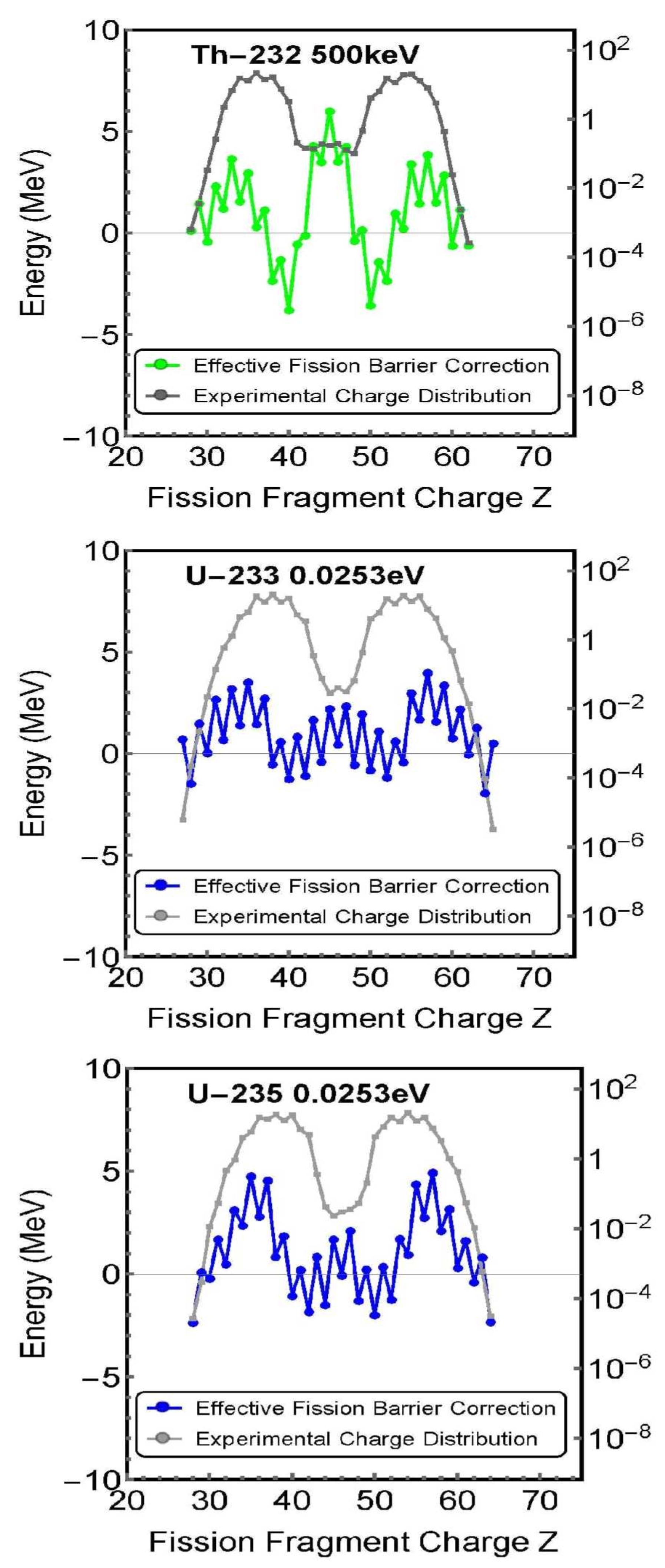
Figure 8.
Effective fission barrier corrections (calculated values) and charge distributions of .
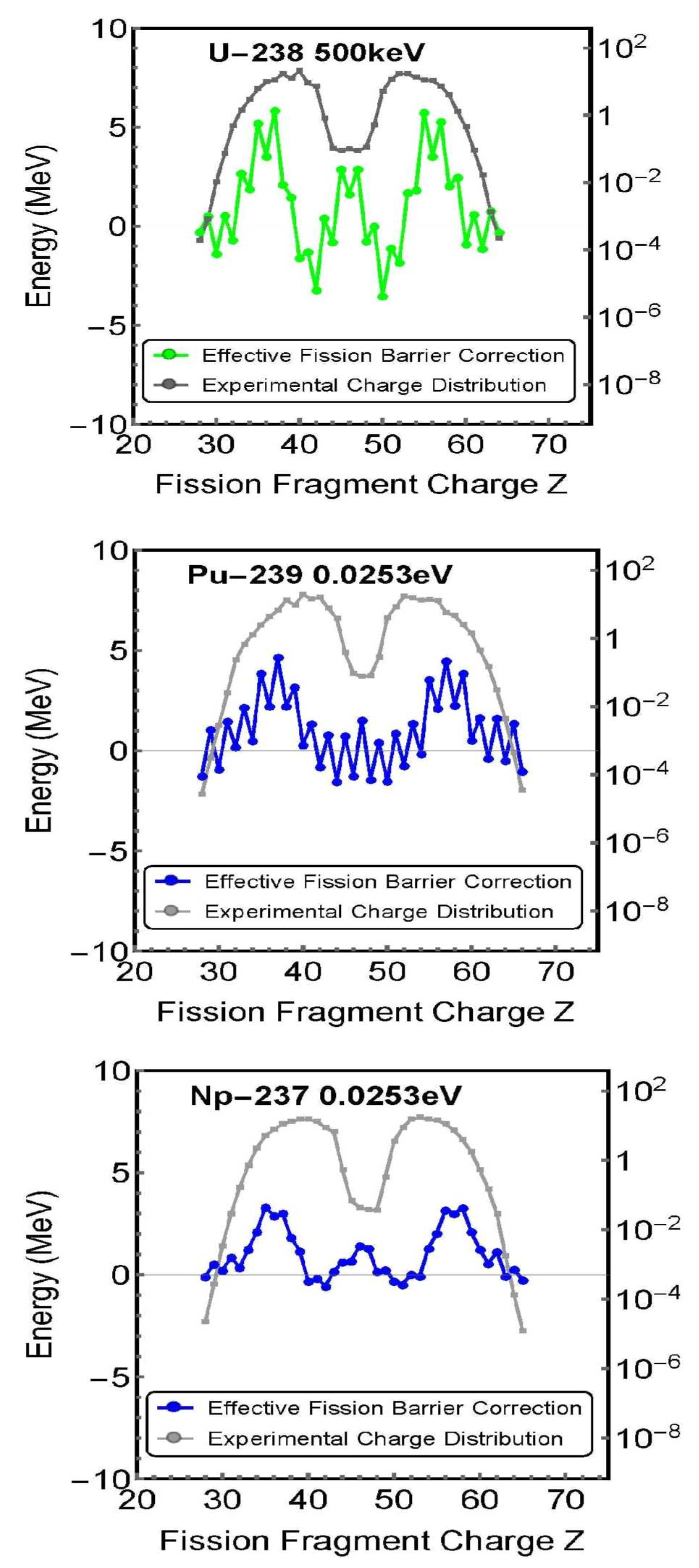
Figure 9.
Effective fission barrier corrections (calculated values) and charge distributions of .
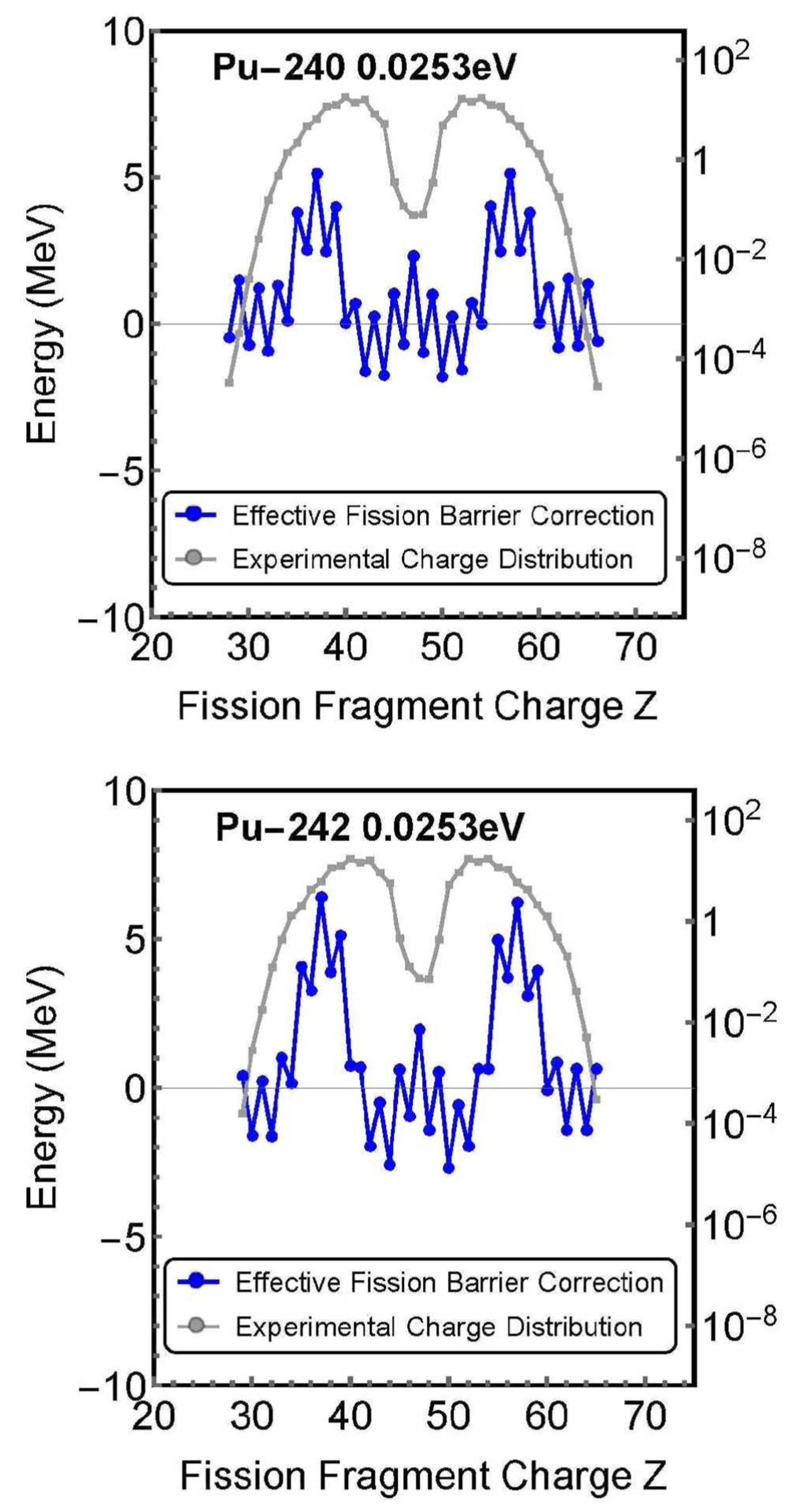
Figure 10.
Schematic representation of the harmonic oscillator model for nuclear fission. The atomic nucleus is modeled as two fission fragments (FP1 and FP2) connected by an ideal spring, where the charge numbers Z1 and Z2 are used instead of masses in the harmonic oscillator treatment.
Figure 10.
Schematic representation of the harmonic oscillator model for nuclear fission. The atomic nucleus is modeled as two fission fragments (FP1 and FP2) connected by an ideal spring, where the charge numbers Z1 and Z2 are used instead of masses in the harmonic oscillator treatment.
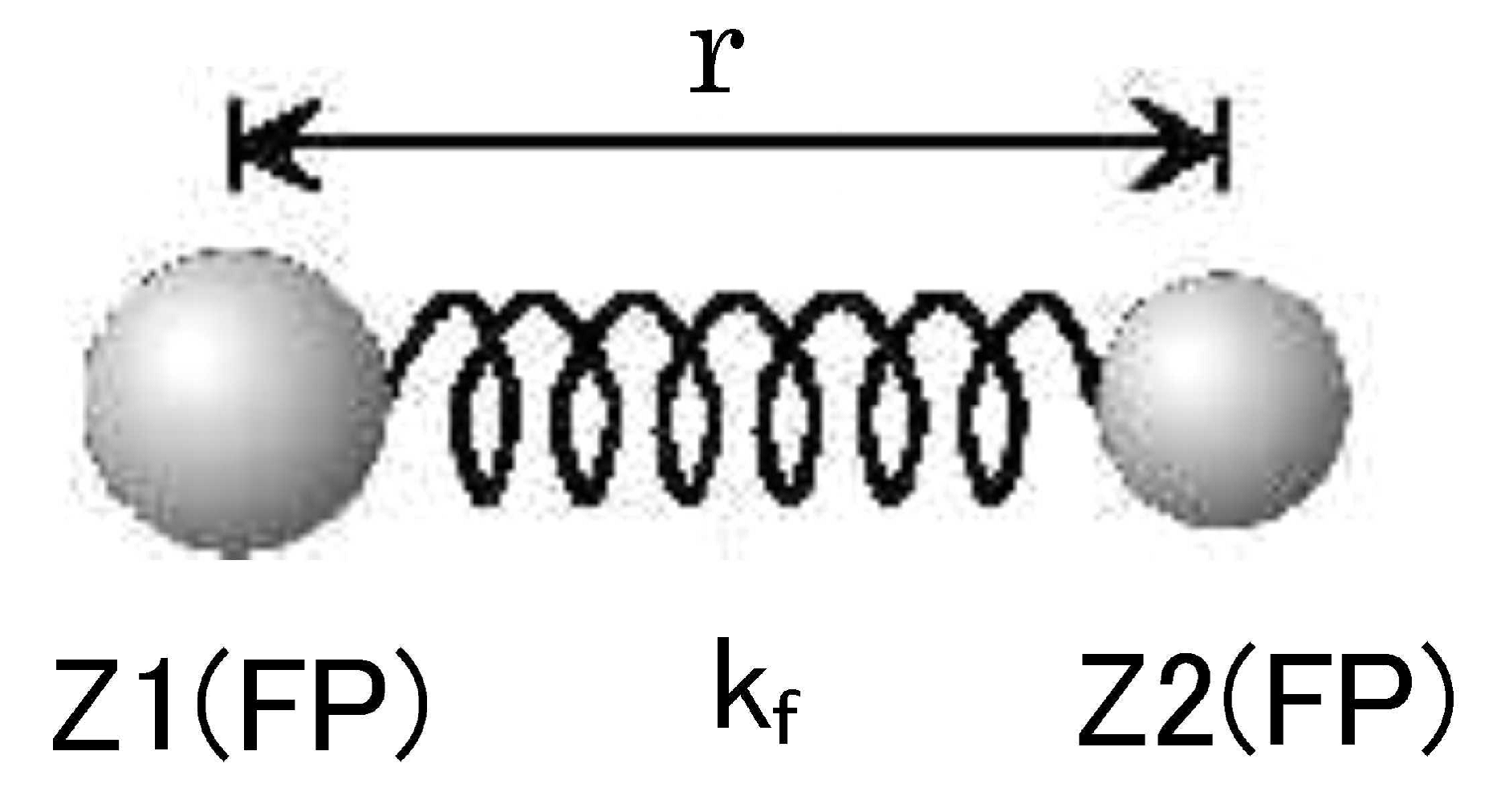
Figure 11.
Relationship between nuclear fission process, potential energy, and effective scission distance . The diagram illustrates how the potential energy changes during the fission process and the definition of effective scission distance at the point where Coulomb repulsion becomes dominant.
Figure 11.
Relationship between nuclear fission process, potential energy, and effective scission distance . The diagram illustrates how the potential energy changes during the fission process and the definition of effective scission distance at the point where Coulomb repulsion becomes dominant.
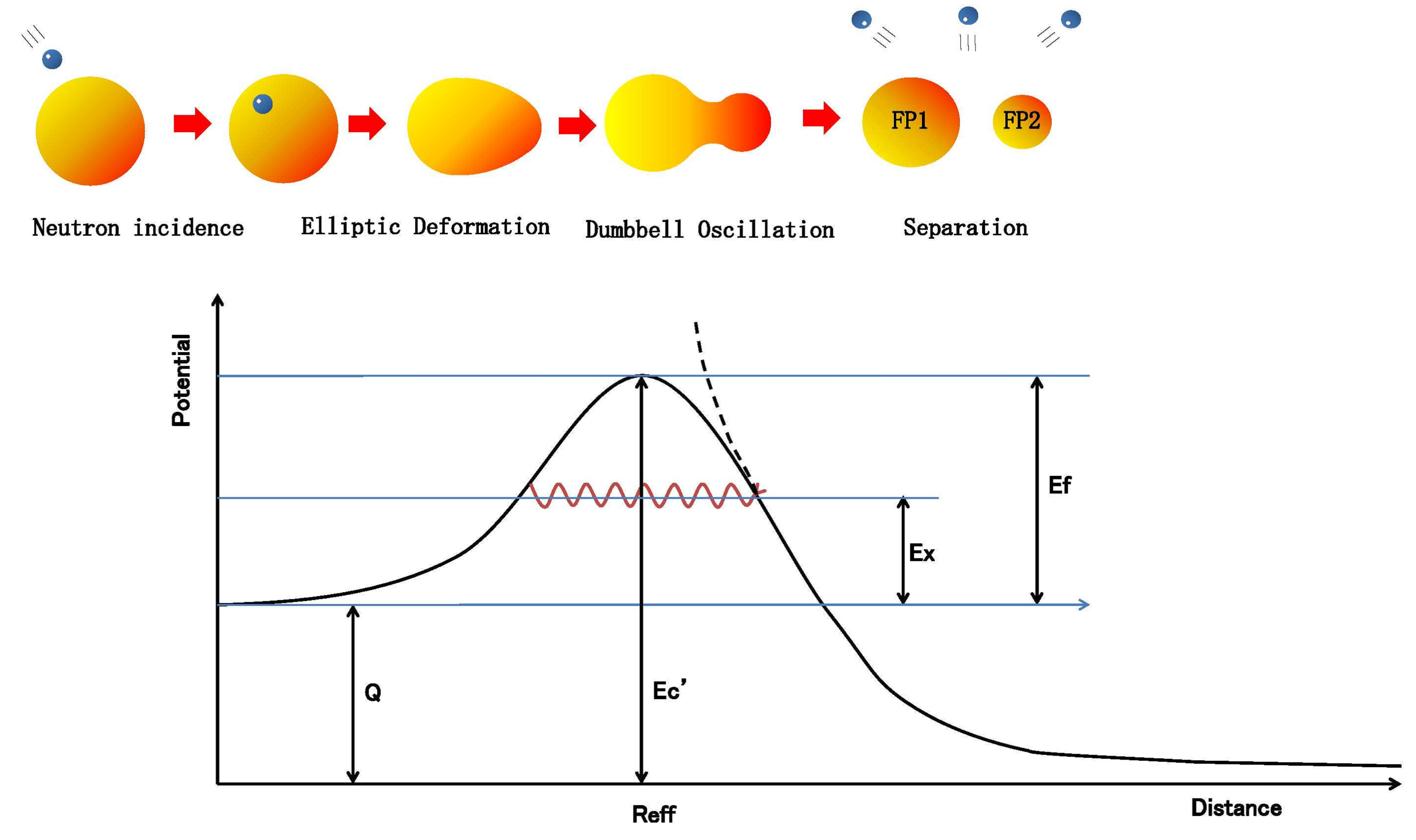
Figure 12.
Nuclear potential energy as a function of radius, showing the rapid weakening of nuclear force at approximately 1 fm. The calculated potential demonstrates the transition region where nuclear force diminishes and Coulomb repulsion becomes the dominant interaction.
Figure 12.
Nuclear potential energy as a function of radius, showing the rapid weakening of nuclear force at approximately 1 fm. The calculated potential demonstrates the transition region where nuclear force diminishes and Coulomb repulsion becomes the dominant interaction.
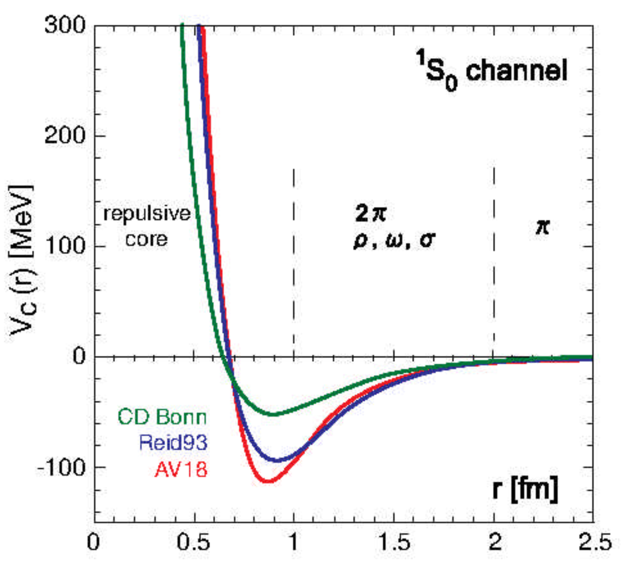

Table 1.
Eight types of target nuclei used in calculations and calculation conditions.
| Target | Neutron separation | Incident neutron | Number of generated |
| nucleus | energy | energy | neutrons (average value) |
| +n | 4.7863MeV | 500keV | 2 |
| +n | 6.8455MeV | 0.0253eV | 2 |
| +n | 6.5455MeV | 0.0253eV | 2 |
| +n | 4.8063MeV | 500keV | 2 |
| +n | 5.4882MeV | 0.0253eV | 3 |
| +n | 6.5342MeV | 0.0253eV | 3 |
| +n | 5.2415MeV | 0.0253eV | 3 |
| +n | 5.0336MeV | 0.0253eV | 4 |
Table 2.
Comparison of reaction equations where effective fission barrier correction is maximum and neutron separation energy.
Table 2.
Comparison of reaction equations where effective fission barrier correction is maximum and neutron separation energy.
| A.Reaction equation of | B.Critical | C.Neutron | C-B | E.Nuclear |
| maximum correction value | energy | separation | fission | |
| (:0.0253eV,:500keV) | (MeV) | energy (MeV) | (MeV) | cross-section |
| +→ Rh+Rh+2n | 6.0 | 4.8 | -1.2 | 53.71b |
| +→ Br+La+2n | 3.8 | 6.8 | +3.0 | 531.3b |
| +→ Br+La+2n | 4.9 | 6.5 | +1.6 | 585.1b |
| +→ Rb+Cs+2n | 5.8 | 4.8 | -1.0 | 16.803b |
| +→ Br+Ce+3n | 3.3 | 5.5 | +2.2 | 20.19mb |
| +→ Rb+La+3n | 4.6 | 6.5 | +1.9 | 747.4b |
| +→ Rb+La+3n | 5.2 | 5.2 | 0.0 | 36.21mb |
| +→ Rb+La+4n | 6.4 | 5.0 | -1.4 | 2.436mb |
Disclaimer/Publisher’s Note: The statements, opinions and data contained in all publications are solely those of the individual author(s) and contributor(s) and not of MDPI and/or the editor(s). MDPI and/or the editor(s) disclaim responsibility for any injury to people or property resulting from any ideas, methods, instructions or products referred to in the content. |
© 2024 by the authors. Licensee MDPI, Basel, Switzerland. This article is an open access article distributed under the terms and conditions of the Creative Commons Attribution (CC BY) license (http://creativecommons.org/licenses/by/4.0/).
Copyright: This open access article is published under a Creative Commons CC BY 4.0 license, which permit the free download, distribution, and reuse, provided that the author and preprint are cited in any reuse.


