1. Introduction
The diversity of wind conditions, i.e. of wind energy potential, has not only a regional character (Coastal, Greater Poland, Mazovia, Suwałki Region) but also a local one related to the local terrain and urban development. The opportunity to increase energy potential on a macro and micro scale can be exploited through the use of small or micro wind power plants [
1,
2].
The location of zones favourable for wind energy development is based not so much on the annual average wind speed as on an analysis of the frequency of occurrence of particular wind speeds in a specific area (regional or local) [
1]. This measured frequency of occurrence of the limiting wind speed for the estimated profitability of wind power plants (4
) is a criterion for the implementation of a specific technical and organisational solution. The variability in the frequency of the different wind speeds does not only relate to the seasons but also to the intensity of solar radiation during the day. The shift in the day time of peak electricity production and increased demand creates the problem of energy storage or sell it back to the external grid. In addition to these three issues, i.e. the location of zones favourable for wind speed, the frequency of its changes and the need for local storage and cooperation with the external power grid, the independence of wind turbine operation from the variability of the direction from which the wind is blowing is also important. Most types of modern wind turbines operate independently of the direction of the prevailing winds in Poland (westerly and south-easterly). Information about this dominance allows optimising the location of urban micro wind turbines [
3,
4].
It should be remembered that the wind speed and direction (their variability) depend on many factors and are random in nature, difficult to predict (e.g. several hours in advance). The dependence of the power of the wind stream flowing through the area circled by the blades of a wind turbine can be described by a dependency model, in which the wind speed and the density of the flowing air play the significant role [
5,
6].
The power at the rotor shaft is lower than the wind power in front of the turbine, which can be determined using the wind energy conversion efficiency index dependent on the construction design of the wind turbine. The relatively high efficiency of the above mentioned conversion is characterised by today’s most popular three-platform designs with a horizontal axis of rotation. The disadvantage of this solution is the need for a homing mechanism depending on wind direction and a second mechanism to slow down the rotation in strong winds, ensuring that the threshold for safe wind turbine operation is not exceeded.
An alternative solution is vertical turbines that operate over a wide range of speed parameters and independently of wind direction. The lower speeds of this solution have a higher efficiency and the power utilisation factor is also lower than with horizontal turbines. An opportunity to increase the amount of power generated from vertical turbines is the use of sets of vertical turbines assembled into a panel [
7] or wall [
8], which can be used as fences or delineators between lanes on motorways. That kind of solutions are not yet well described in the literature.
Summarising, it can be stated that there are two key problems in the implementation of low-power wind turbines. The first is the logistical issue of their location in urban conditions. This issue requires an apriori verification of local wind data in order to select a technological and organisational solution that determines the optimum dependence of the electric power produced by the turbine on the aforementioned conditions of long-term variability of power, wind speed and direction and air density. A solution that locally stores or resells the generated energy to an external grid is also important. The second issue that the authors focus on in presented article is to learn the characteristics and amount of power generated by low-power wind turbines, especially those located at short distance from each other.
2. Materials and Methods
2.1. Geometrical model
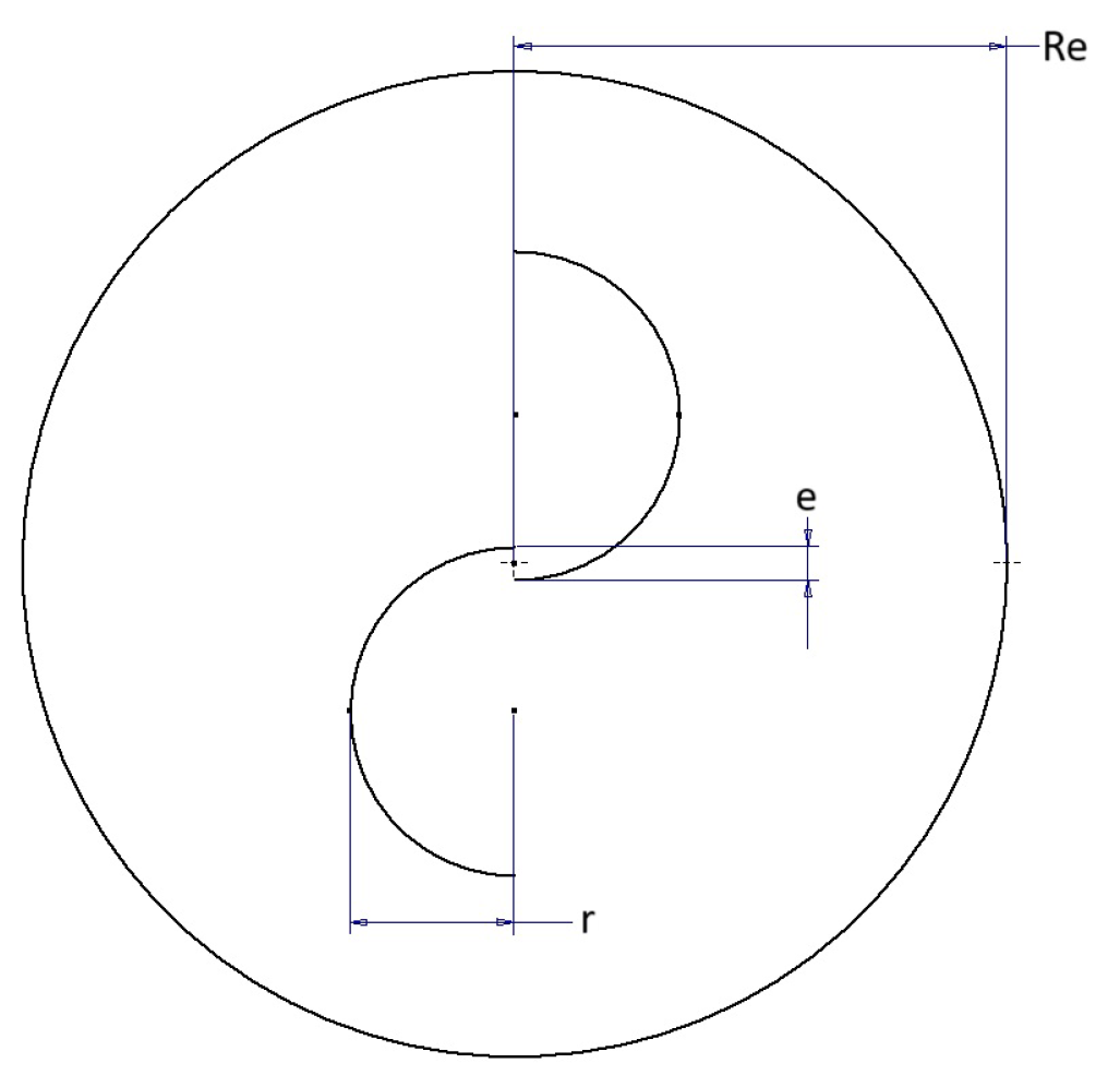
A geometrical model of the turbine was prepared with dimensions given in
Table 1. Figure
Table 1 shows the geometry of a single turbine. Despite examples of using other blade shapes, as shown in [
9,
10], the blades were made as half circles. The domain of single turbine was 30D lenght and 8D width. For a panel, distance between turbine axis was set to 1.974D (0.75 m), and there were six turbines in a row. The whole domain was 66D lenght and 40D width.
Figure 1.
Dimension of the turbine and rotating domain.
Figure 1.
Dimension of the turbine and rotating domain.
2.2. Numerical Model
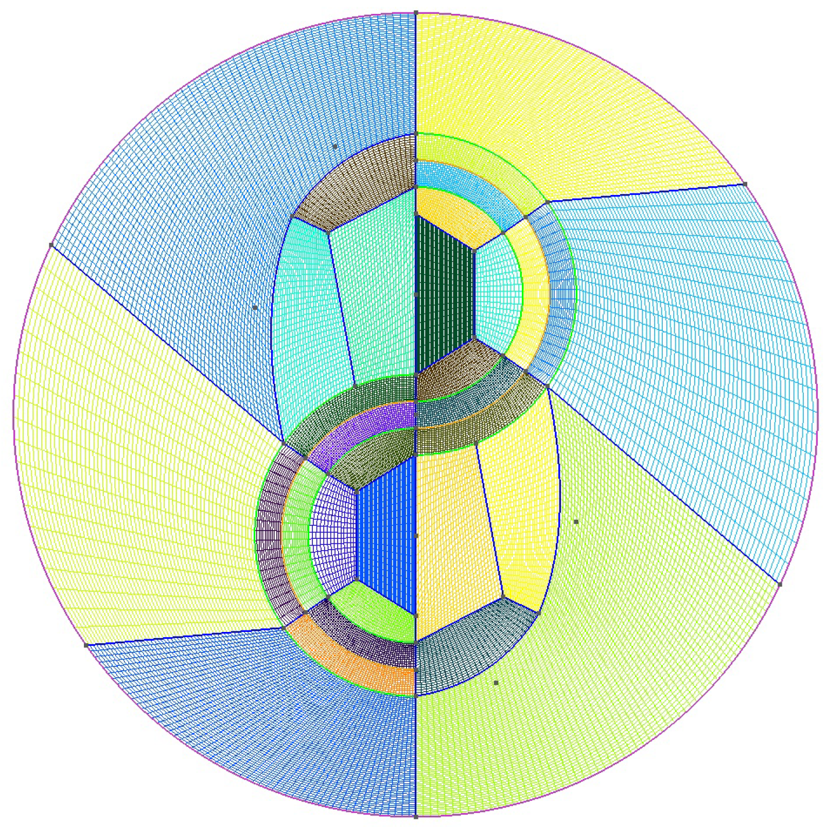
Based on a geometry showed in Figure
Table 1 a mesh for CFD calculation was prepared. Firstly a mesh for single turbine was prepared for calculate based values. After that a mesh for a whole panel was build. Mesh for a single turbine is shown in
Figure 2 and it has 33880 elements. Domain for the single turbine has 70308 elements and for the wind panel - 378573 elements. For each case the mesh was build with 2D qaudrilateral elements. For both, single turbine and wind panel, turbine blades were modeled as zero-thickness wall. Calculations were performed as unsteady RANS with
SST turbulence model and standard atmospheric conditions.
The rotating domain for turbines were set as mesh motion with axis of rotation individual for each turbine and rotational velocity equal 360.
Authors in [
11] performed calculaton on 7 revolution and authors in [
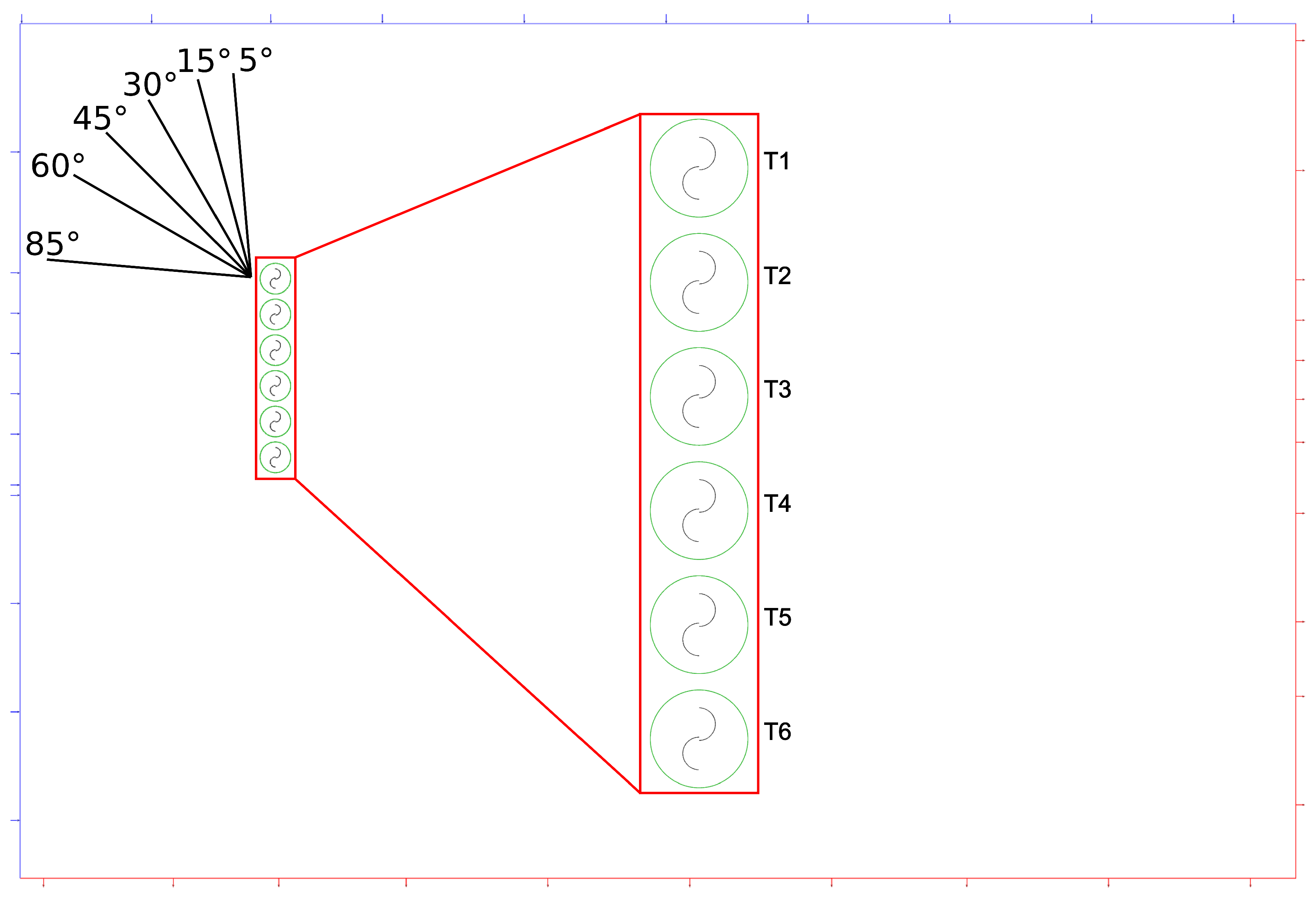
10] - 12.5. Based on that and controling parameter during calculation a 9 rotation were selected. The inlet velocity was set to 10
and the angles of inflow were changed for different cases. The angles were shown in
Figure 3.
Time step was calculated as it was presented in [
12]. Equation (
1) describe the time for sliding mesh cases, and it should not be larger than time takes for a moving cell. In that case characteristic lenght
was equal 0.0004m and velocity
V was equal 0.596
and it resulted time step
. Equation (
2) takes number of blades as one of the parameter and it gaves time step
. For the presented calculation the time step was set to
from the begining to the 8th rotate which correspond to 1
of rotation. The last rotate was calculated with time step equal
which correspond to 0.5
of rotation. Data for the analysis was taken from last 3 revolution.
3. Results
As the reference a maximum available energy from the wind was calculated based on Equation (
3). By knowing the turbine diameter (0.38 m) and reference value for height in 2D calculations (1 m), the maximum available power was equal 238.88 W.
The numerical analysis in Ansys Fluent allows to control and save parameters of force and torque on the wall. For presented analysis a generated torque on each turbine was stored seperately for each time step. By using Equations (
4) and (
5) the instantaneous power were calculated. Following that a peak and mean power were calculated. From Equation (
6) power coefficient were calculated.
The values for reference single turbine were presented in
Table 2.
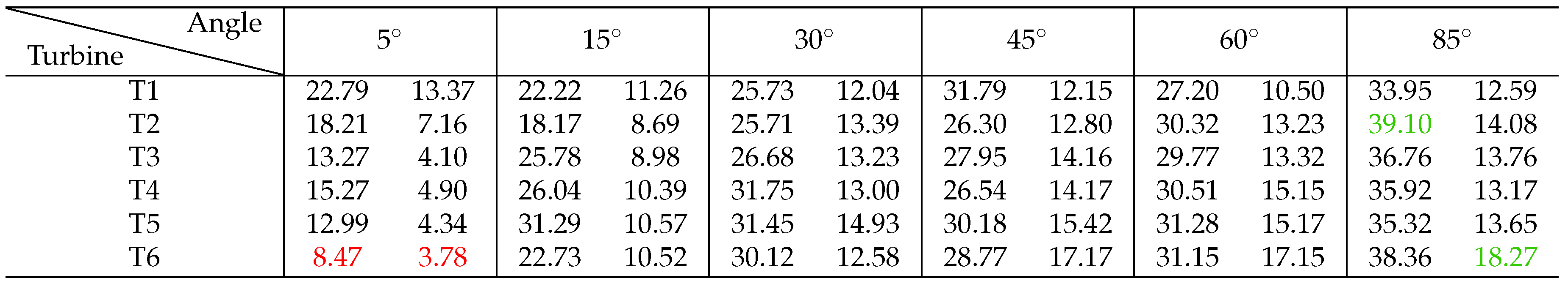
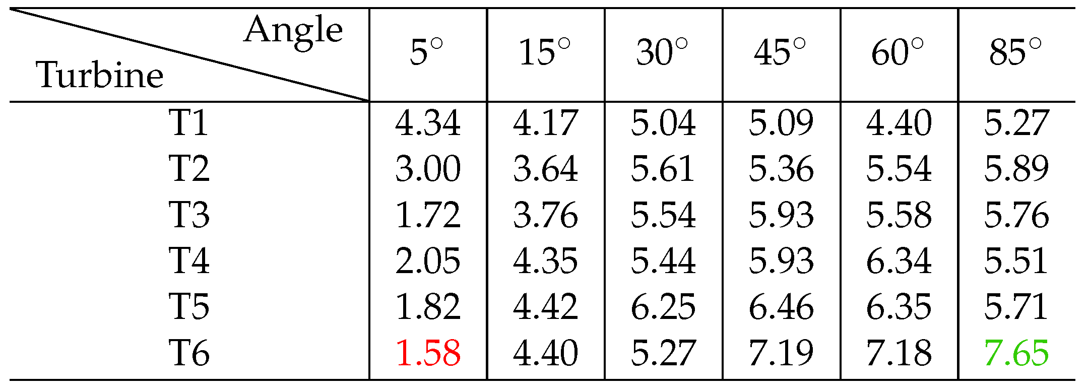
Below a result from panels is presented. A peak and mean power are in
Table 3 and power coefficient in
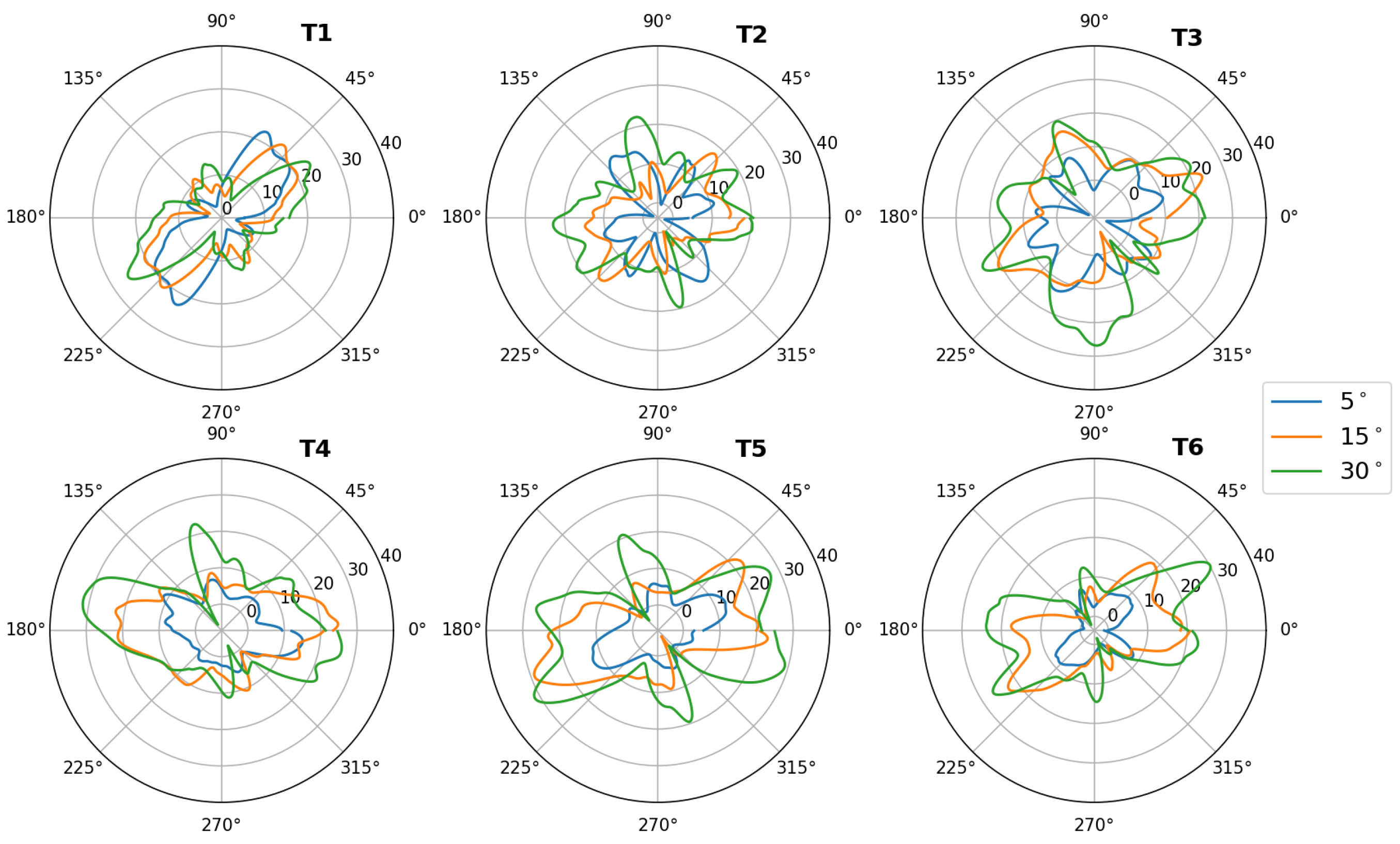
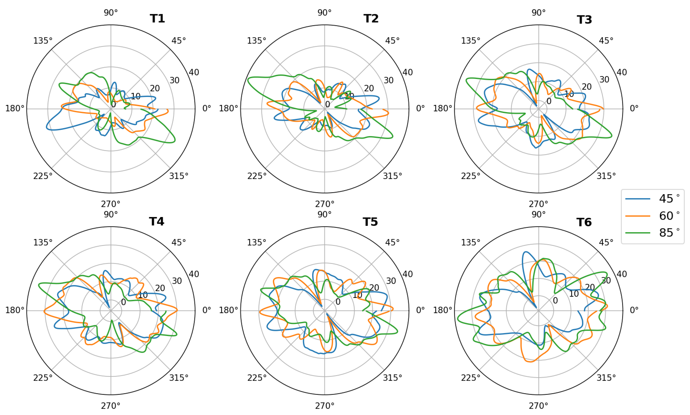
Table 4. In both tables maximum and minimum values were marked with, accordingly, green and red color. It can be noticed, that values in wind panel are lower than a single turbine. It is caused by the direct wake from preceding turbines, for low inflow angles, and to a lesser extent from turbulence between turbines for high inflow angles.
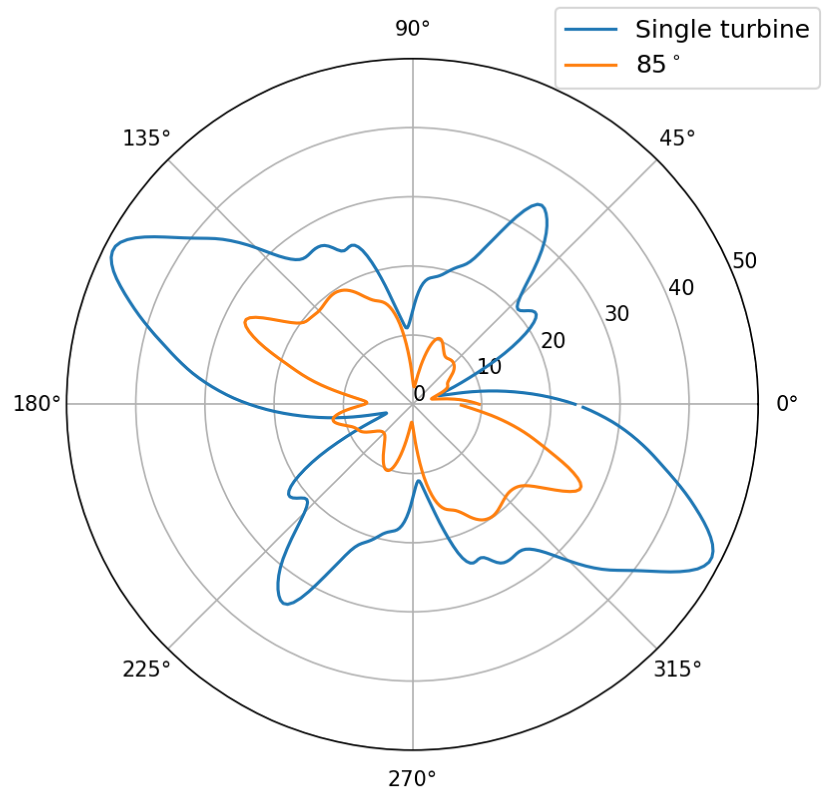
The large disproportion in the unevenness of power delivery is visible in the
Figure 4,
Figure 5 and
Figure 6. The
Figure 4 shows the power values for the reference case and for the first turbine with an inflow angle of 85
. It can be seen that the shape of the curve is very similar, with clear power peaks at the moment of optimal turbine direction to receive energy from the wind. Similar relationships can be seen in the discussed figures for turbine T1. Additionally, a shift in the inflow direction by an angle of 80
is clearly visible. The subsequent graphs in the discussed figures do not have such a clearly outlined shape, and additionally, despite the symmetry of the turbine and the expected symmetrical power output on each of the blades, the maximum values do not occur opposite each other and their values are different.
4. Discussion
Analyzing the presented results, one can conclude that the flow between them has a very large impact on the amount of energy produced by individual turbines. For the case with an inflow angle of 5, the amount of energy produced along the panel decreases, however, looking at the other cases, we do not have such a sudden drop in efficiency on the subsequent turbines. It is also worth noting that the first turbine in the row does not generate the highest power in the entire panel. In the case of an inflow angle of 85, which is the closest to the perpendicular, one could expect uniform operation of all turbines, significant differences between the amount of energy produced by them can be seen. It should also be taken into account that the calculations were prepared and performed in two-dimensional space and, additionally, the last rotation that was analyzed was performed with a time step equal to half a degree, while the previous 2 were performed with a time step equal to one degree of the turbine rotation angle. This may also be important in the context of the flowing fluid, especially if we accept for analysis the case in which a single turbine was presented with undisturbed flow around it. Analyzing the average power generated by the turbine in the case of an inflow angle of 85, the highest power was obtained by turbine number 6. The authors presume that this is due to the inflow of additional air from turbine number 5 during its rotation. The presented results show that the amount of generated energy with the increase of the inflow angle will change in favor of the one closer to the perpendicular, however, the amount of energy produced individually by each turbine will not be the same as in the case of a single turbine positioned far from obstacles. The next stages of work are to change the geometry to fully three-dimensional, even greater mesh density and change the turbulence model and calculation method to LES or DES in order to increase the accuracy of the obtained results. It will also be important to conduct an experiment in a wind tunnel for the presented turbines with the possibility of changing the angle setting in order to obtain the input parameters such as those presented in this article.
Author Contributions
Przemyslaw Grzymislawski and Dawid Poltoraczyk prepared geometry, mesh, performed CFD simulations and analyse data, Przemyslaw Grzymislawski and Joanna Kalkowska wrote the paper. All authors have read and agreed to the published version of the manuscript.
Funding
This research received no external funding.
Conflicts of Interest
The authors declare no conflicts of interest.
Abbreviations
The following abbreviations are used in this manuscript:
| CFD |
Computational Fluid Dynamics |
| RANS |
Reynolds Averaged Navier-Stokes |
| RPM |
revolution per minute |
References
- Cichoń, A.; Malinowski, P.; Mazurek, W. Porównanie możliwości wykorzystania małych turbin wiatrowych o poziomej i pionowej osi obrotu. Przeglad Elektrotechniczny 2016, 92. [Google Scholar] [CrossRef]
- Poplawski, T. Problematyka prognoz generacji wiatrowej w KSE. Przeglad Elektrotechniczny 2014, 90, 119–122. [Google Scholar]
- Boczar, T.; Szczyrba, T. Ocena wpływu warunków meteorologicznych na sprawność turbin wiatrowych. Pomiary, Automatyka, Kontrola 2012, 58, 1044–1047. [Google Scholar]
- Jarzyna, W.; Pawłowski, A.; Viktorich, N. Technological development of wind energy and compliance with requirements for sustainable development. Problems of Sustainable Development 2014, 9, 167–177. [Google Scholar]
- Farrugia, R. N. The wind shear exponent in a Mediterranean island climate. Renewable Energy 2003, 28, 647–653. [Google Scholar] [CrossRef]
- Firdaus, B.; Izwan, I.; Thamir, K. I.; Daing, M. N. D. I.; Shahrani, A. A study on the power generation potential of mini wind turbine in east coast of Peninsular Malaysia. AIP Conference Proceedings 2017, 1826. [Google Scholar]
- VINDPANEL. Available online: https://www.vindpanel.com/ (accessed on 17 November 2024).
- New Atlas. Available online: https://newatlas.com/energy/wind-turbine-wall-doucet/ (accessed on 17 November 2024).
- Zemamou, M.; Aggour, M.; Toumi, A. Review of savonius wind turbine design and performance. Energy Procedia 2017, 141, 383–388. [Google Scholar] [CrossRef]
- Im, H.; Kim, B. Power, Performance Analysis Based on Savonius Wind Turbine Blade Design and Layout Optimization through Rotor Wake Flow Analysis. Energies 2022, 15, 9500. [Google Scholar] [CrossRef]
- Mohamed, M.; Dessoky, A.; Hafiz, A. A. CFD analysis for H-rotor Darrieus turbine as a low speed wind energy converter. Engineering Science and Technology, an International Journal 2014, 18. [Google Scholar] [CrossRef]
- Alaimo, A.; Esposito, A.; Messineo, A.; Orlando, C.; Tumino, D. 3D CFD Analysis of a Vertical Axis Wind Turbine. Energies 2015, 4, 3010–3033. [Google Scholar] [CrossRef]
|
Disclaimer/Publisher’s Note: The statements, opinions and data contained in all publications are solely those of the individual author(s) and contributor(s) and not of MDPI and/or the editor(s). MDPI and/or the editor(s) disclaim responsibility for any injury to people or property resulting from any ideas, methods, instructions or products referred to in the content. |
© 2024 by the authors. Licensee MDPI, Basel, Switzerland. This article is an open access article distributed under the terms and conditions of the Creative Commons Attribution (CC BY) license (http://creativecommons.org/licenses/by/4.0/).