
Submitted:
25 November 2024
Posted:
26 November 2024
You are already at the latest version
Abstract
This contribution investigates whether the use of the MATLAB optimization toolbox on a parameter identification problem for a TRNSYS model provides an advantage.There it presents the development of a framework interconnecting MATLAB Optimization Toolbox with TRNSYS on the one hand side and coordination of the optimization process of a TRNSYS model by GenOpt through MATLAB on the other hand. A benchmark script in MATLAB was created to link TRNSYS and MATLAB and to configure the optimization process of GenOpt and MATLAB Optimization Toolbox. Using this framework, a comparison of the optimization solvers in GenOpt and MATLAB Optimization Toolbox for the identification of the overall heat transfer coefficient of a TRNSYS heat exchanger model regarding the optimization time and numbers of iterations will be presented as a use case. The results for the given problem show that GenOpt gives slightly better results in optimization time whereas MATLAB has more potential and flexibility of parameter tuning.
Keywords:
TRNSYS
; MATLAB
; GenOpt
; co-simulation
; optimization
; tool coupling
1. Introduction
Control of Building Energy Systems (BES), which is part of the Building Automation and Control System (BACS), and model-based design is a complex task comprising different domains and has increasingly become established in energy industry and research. Nevertheless, these systems can further be improved by optimal design and control to be more cost effective and reliable.
A large number of Building Performance Simulation Tools (BPSTs) have been developed in the last decades [1]. A comprehensive list of BPSTs is provided in [2].
One reason for the increasing use of BPSTs is not least the increased legal requirements for BES. The revised Energy Performance of Buildings Directive (EPBD) (EU/2024/1275) entered into force in all EU countries on May 2024. An entire set of rules is applied here, for which EN 15322-1 is used in sub-module M10 (Building Automation and Controls), in which the building is assigned to one of four BACS efficiency classes [3]. The amended version introduces new requirements for non-residential and residential buildings, which should help to accelerate the gradual renovation of the entire building stock. In Germany, the new Building Energy Act (GEG 2023) regulates how the country will heat predominantly with renewable energies (RE) in the future. The GEG 2023 aims to increase the share of renewable energies in buildings sustainably and efficiently. According to the new requirements, new buildings BES will only be installed if they generate at least 65% of the heat provided using RE.
BPSTs are used in research and increasingly also in industry. They have different levels of model detail and cover the entire life cycle of a BES, from the design, construction and operation of buildings, to accelerate and improve the design and planning process, improve building efficiency, develop or optimize building controls and evaluate the market potential of new concepts.
At present, there exist domain independent software tools with advanced control modeling features but less building simulation model capabilities and vice versa. Hence, an advanced approach is to combine the different software tools and their modular concept by runtime coupling to incorporate their domain specific advantages as model libraries, optimization algorithms or aided controller design [4].
This paper is organized as follows: Section 2 discusses the most common methods of software coupling to TRNSYS and previous work in a literature review to identify the research gap that this paper aims to close. Section 3 describes the benchmark model implementation in TRNSYS for the one-dimensional optimization problem, the framework of coordinated optimization by GenOpt through MATLAB, as well as using MATLAB optimizer solely with TRNSYS. In Section 4, the chosen solver parameters are listed, and the performance results are shown and discussed. A summary of the main findings and an outlook on further work concludes the contribution in Section 5.
2. Related Work and Research Question
In this study, the focus was placed on TRNSYS as a commonly used BES modeling tool. In the following, possible tool coupling methods are listed and briefly explained. Furthermore, the results of a literature search are listed in order to be able to classify the content of this article in the research gap and to be able to formulate the research question.
2.1. Tool Coupling to TRNSYS
Several interfaces between simulation software tools have been developed or tested for tool coupling or co-simulation [5,6,7]. Coupling between different software tools can be implemented either in a strong or a loose way [8]. In strong coupling, the models of all the connected simulators iterate in each simulation time step until they converge. This shows higher accuracy at cost of higher computational load. Contrary to this in loose coupling the exchange data is only transmitted at the beginning of each time step and the feedback between the simulators is lags by one simulation time step. In the following, some methods of tool coupling, especially between MATLAB and TRNSYS, are described.
Building Controls Virtual Test Bed (BCVTB)
BCVTB is an open-source framework for co-simulation and acts as a middleware between several software tools like e.g. TRNSYS, MATLAB, Dymola and EnergyPlus as well as the Functional Mock-up Interface (FMI) [9]. Data exchange between the tools is implemented through socket communication. In [6] a building controller was developed using co-simulation where BCVTB connects MATLAB for controller design and EnergyPlus for building simulation. As a drawback the authors identified the high simulation time. Furthermore, debugging of the co-simulation proved to be difficult, since BCVTB can only listen to ports.
TRNSYS Type 155
TRNSYS has also its build-in support of external programs. Beside Microsoft Excel, ANSYS Fluent, ESP-r, Java and some more, it can also directly communicate with MATLAB via Type 155. This Type implements a connection to the MATLAB engine in a separate process through the Component Object Model (COM) concept. Type 155 can be used in two different calling modes, iterative mode (strong coupling) and real time controller mode (loose coupling). A thermal use case example to compare the computational efficiency and accuracy had been published in [7]. The authors stated higher flexibility to the user in comparison to BCVTB and FMI.
Open Platform Communications Unified Architecture (OPC UA)
OPC UA is a platform independent service-oriented architecture communication standard. It serves information interchangeability between real controller as well as software tools. While MATLAB has a build in OPC Toolbox, TRNSYS is lacking of this interface. In [10], Pan et al. give no details about the implementation.
TCP/IP
Using this communication protocol, tools are enabled to have a general interface. While MATLAB offers functions to create TCP/IP client and server, TRNSYS does not and the user has to create a custom type as shown in [11].
Functional Mock-up Interface (FMI)
FMI is an open standard software tool interface for exchanging simulation models. While exporting a model to a Functional Mock-up Unit (FMU) the resulting fmu file incorporates an xml description file and compiled c-code in a dll file. FMU import in Simulink is supported since version 2017b by an FMU import block. Importing and exporting FMUs is available through an additional toolbox [12]. Within TRNSYS only FMU export is available using an open source adapter called Type 6139 [13].
Dynamic Link Library (DLL)
TRNSYS Type 163/169 (CFFI)
The TRNSYS standard Type 163 and Type 169, enable the transfer of TRNSYS simulation model states to Python. The two calling Python types differ fundamentally from each other. Type 163 reads and writes files between TRNSYS and Python at each simulation step. Type 169, which is coded in C++, uses the C-API principle of Python for direct communication interface. Although it embeds Python in the code, it requires extensive C wrapper code to enable direct communication between TRNSYS and Python.
TRNSYS Type 3157 (CFFI)
Compared to Type 169, the communication with the Python script has been significantly improved in Type 3157. This package calls a Python module at runtime, which is implemented in a Python file located in the same directory as the TRNSYS input file (the deck file). This script can use any package or library installed in the Python environment. Communication between the (Fortran) TRNSYS DLL and the Python environment takes place via a Foreign Function Interface, which is defined using the CFFI Python package [16].
File Input/Output (FIO)
The TRNSYS simulation engine can be directly executed via command prompt by typing:
Path_to_TRNExe.exe\TRNExe.exe Path_to_Dck_file\Dck_file.dck \switch
where switch can be:
- n : This skips the dialog boxes that inform the user at the end of simulation on errors during the simulation process and therefore enables a batch mode.
- h : This implies the n-switch and enables the hidden batch mode that makes TRNSYS completely invisible. Graphical output by online plotter is not possible and has to be disabled by setting parameter 9 of the online plotter to -1. As an advantage the simulation will be speed-up noticeably.
By modifying the deck file using text editors, model parameters can be changed automatically in order to carry out parameter studies . It can also be used to create entire models, as is possible with pytrnsys [17]. In this context, TRNSYS printer types can be added to the model, for example, to generate an output file that can in turn be used as an input in the optimization loops for optimization processes as it is the principle in GenOpt [18].
In this study, the FIO approach is also used to determine a model parameter in an optimization problem by means of error minimization. A TRNSYS-MATLAB framework was developed to enable the automated iteration process.
2.2. Review
There are several studies in the literature that have either examined the coupling of the various BPSTs or compared them with each other in terms of accuracy and runtime using a reference model.
Solmaz [19] provided a critical overview of the developments in the field of BPSTs in the study and evaluated the effectiveness of nine BPSTs in the design process. A group of validated and accurate BPSTs were examined, categorized and compared based on general characteristics, validation, interoperability, user adaptation, application/functions, strengths and limitations. The BPSTs were divided into two groups. The first group consists of planning tools such as Revit, Rhino and SketchUp, the second of detailed simulation tools such as EnergyPlus, DOE2 and TRNSYS. In addition, there is other software (OpenStudio, DesignBuilder, Green Building Studio) that uses the simulation programs of the other tools.
In their review, Barber and Krarti [20] examined the common optimization tools for the design and control of building energy systems and their combined use. They looked at multi-objective optimization problems and showed the typical flowcharts of the approaches used. The software tools were divided into three categories: simulation engines, graphical user interfaces and simulation environments. TRNSYS was assigned to the first category and MATLAB to the third. According to the authors’ classification, the main difference between simulation engines and environments is that the latter contains several plug-ins or features, while the former are essentially standalone programs.
TRNSYS (TRaNsient SYstem Simulation Program) [21] is one of the BPST, which is well known for its numerous validation studies and its ability to model buildings incorporated with other systems, such as HVAC and renewable energy sources for dynamic system simulation based on numerical routines solving partial differential equation systems. It enables the balancing of transient processes in a time step resolution between hours and minutes. It has a modular structure comprising of modules like multi-zone buildings and electrical and thermal energy systems. A disadvantage of TRNSYS is the missing of user friendly integration of complex control and optimal system sizing methods.
MATLAB (MATrix LABoratory) is a simulation environment for programming and numerical calculations [22] with its hugh variety of toolboxes, e.g. Optimization Toolbox and Parallel Computing Toolbox.
Magni et al. [23] described the modeling approaches of eight widely used BPSTs in their work and compared them on a monthly and hourly basis for the climate zones Stockholm, Stuttgart and Rome using simulation results for the same office cell defined by IEA SHC Task 56. The results of the cross-comparison show that overall a good match was achieved between all dynamic simulation tools. The simulation with EnergyPlus was the fastest, followed by TRNSYS and ALMABuild. The authors also emphasized that it took several iterations and great effort on the part of the modelers to achieve a good match between all tools.
In their paper, Mazzeo et al. [24] compare three common simulation tools for building simulation, namely EnergyPlus, IDA ICE and TRNSYS, with the experimental data of two solar test boxes equipped without and with a PCM material in the floor, in three different warm, intermediate and cold periods. Measurements of the internal air temperature, the internal and external surface temperature of the glass and the internal surface temperature of the floor are used for this purpose. Their results show that the three tools are very comparable in the absence of PCM. TRNSYS has the highest accuracy in the warm period, while this is the case for IDA ICE in the cold period. Overall, IDA ICE is the best tool in all periods. In the presence of PCM, it can be seen that IDA ICE achieves almost the same accuracy as can be achieved without PCM, while the other tools deliver lower accuracies.
Kalkan et al. [25] compared the simulation time for an absorption chiller and PVT collector model programmed in C++, MATLAB and Python and integrated into TRNSYS using Type 155 and Type 3157 respectively. Their results show that the simulation speed decreases significantly from C++ to Python to MATLAB. The authors recommend the use of Python if MATLAB libraries do not have to be used explicitly.
Some research has been done by applying free available software tool GenOpt (Generic Optimization Program) [18] in order to automate TRNSYS runs and to minimization a cost function also supporting parallel computing optimization. However, GenOpt is not capable of handling multi-objective optimization. When associated with TRNSYS, GenOpt can automatically generate building (.bui) and deck (.dck) files, run TRNSYS with those files save results, and restart again.
Fernandes et al. [26] presented in their work the methodology and results of a simulation-based optimization and evaluation study of an adsorption storage system in combination with a solar collector system, which was carried out in TRNSYS and MATLAB. The absorption storage components were modeled in MATLAB and integrated into the TRNSYS model with hot water storage tank. Parameter optimization was performed with the GenOpt, which can be coupled with TRNSYS to perform automated parameter variation. The Generalized Pattern Search (GPS) algorithm was used. Twelve parameters were varied with the aim of minimizing the additional heating requirement.
Magnier et al. [27] use a simulation-based artificial neural network (ANN) to characterize building behaviour and then combine this ANN with a multi-criteria genetic algorithm (NSGA-II) for optimization. This methodology was used in the studies to optimize thermal comfort and energy consumption in a residential building. The combination of the two algorithms was called GAINN methodology The simulation model was integrated into TRNSYS. The multi-objective optimization was carried out in two steps. In the first step, a database was automatically generated by varying the model parameters with the help of GenOpt. An ANN was trained on this and the model parameters were optimized using NSGA-II in a second step.
Asadi et al. [28] used a simulation-based, multi-criteria optimization method in their work using a combination of TRNSYS, GenOpt and a Tchebycheff optimization technique developed in MATLAB to optimize the refurbishment costs, energy savings and thermal comfort of a residential building in order to choose the best retrofit strategy for a building.
Since TRNSYS is unable to estimate the effectiveness of evaporation during cooling, which is a typical passive design method, Nayak et al. [29] developed a MATLAB/TRNSYS integration in which TRNSYS was modified to model the simultaneous heat and moisture transport from the damp roof surface of a building. They used the building model (Type 56) and coupled MATLAB with TRNSYS using the Type155. The temperature of the underside of a damp roof calculated with MATLAB was used as the boundary temperature for the dummy roof in TRNSYS.
Narayan et al. [30] developed a coupled simulation framework for the nonlinear, time-varying, deterministic, discrete-time power system problem using TRNSYS and MATLAB. Using this framework, an MPC with a moving horizon of 24 hours was developed for an integrated thermal and electrical system with multiple energy sources in a household optimized for self-consumption. The optimization was carried out using three different algorithms: Particle Swarm Optimization (PSO), Genetic Algorithms (GA) and Global Patternsearch (GPS).
Few publications use the pytrnsys package [17] to automate simulation studies. In their work Arenas-Larrañaga et al. [31], a parametric analysis was carried out using pytrnsys-TRNSYS, taking into account 14 European climate zones, two heat pumps with different natural refrigerants (CO2 and propane), four solar collector areas and three ice storage volumes. The analysis is based on TRNSYS simulations using previously calibrated and validated models. The open source package pytrnsys was used to set up the system visually and to automate the 700 simulations carried out and the post-processing of the data.
The aim of the research work by Mylonas et al. [32] is to demonstrate the reliability, robustness and computational efficiency of a cloud-based application of an MPC called Smart Energy Management for an apartment building. This energy management framework was tested on a virtual building model in TRNSYS running via the pytrnsys package, using an open-source distributed event streaming platform for data exchange and synchronization.
Meiers et al. [33] have proposed a Hardware-in-the-Loop simulation architecture where they describe a communication procedure between TRNSYS, BCVTB and MATLAB as the simulation part and LabVIEW as communication node to the hardware of the real system using Message Queueing Telemetry Transport protocol. BCVTB serves as a middle-ware for the communication between TRNSYS and MATLAB, whereas MATLAB controls the simulation framework itself and ensures the communication to LabVIEW.
2.3. Research Question
The analysis of the reviewed literature shows that there is a research gap with regard to a comprehensive comparison of algorithms for optimizing a TRNSYS model under the aspect of system design (cf. Table 1). This is the starting point for the analysis presented in this contribution. Only the software tools TRNSYS, MATLAB and GenOpt as solver engine or the MATLAB Optimization Toolbox respectively, have been considered here.
Therefore, the main research question is:
Is there an advantage of GenOpt in relation to the creation of a TRNSYS-MATLAB framework due to the possibility of using the algorithms in the MATLAB Optimization Toolbox instead?
In this study, the focus is on model parameter identification by means of an error minimization process using a TRNSYS model. For this purpose, a simple example of a heat exchanger is used to determine the heat transfer coefficient.
The framework for two approaches was developed and the results compared, where both of them are coordinated and automated by MATLAB :
- TRNSYS/GenOpt (TG)
- TRNSYS/MATLAB Optimization Toolbox (TM)
The objective of this study is to address the issues mentioned above in the following key aspects:
- Description of the design of both MATLAB-TRNSYS frameworks, TG and TM respectively, for automated parameterization of models for design optimization and a parameter estimation as a use-case
- Comparison of the required computation times for the estimation process
- Comparison of the solver accuracy for the estimation process
In the following, this contribution focuses on calling TRNSYS model simulation runs via command shell in the FIO approach through MATLAB. An application of the framework described in Section 3 to a multi-objective optimization problem of a BES has already been described by Tadayon et al. [34]. The studies conducted here are limited to a single-objective optimization problem, which is, however, subjected to a more comprehensive comparison of the solvers.

Table 1.
Review Comparison.
| Publication | purpose of tool coupling | tool coupling method with TRNSYS |
used software tools and programming languages |
||||||||
|---|---|---|---|---|---|---|---|---|---|---|---|
| optimization | automation | model extension | parametric analysis | model comparison | |||||||
| design-oriented | operation-oriented | objectives | number and name of solvers |
||||||||
| single | multi | ||||||||||
| Kalkan et al. [25] | - | - | - | - | - | - | xC,P,M | - | - | Type155M Type3157P DLLC |
TRNSYS MATLAB GenOpt C++ |
| Nayak et al. [29] | - | - | - | - | - | - | xM | - | - | Type155M | TRNSYS MATLAB |
| Mazeo et al. [24] | - | - | - | - | - | - | - | - | x | - | TRNSYS EnergyPlus IDA ICE |
| Magni et al. [23] | - | - | - | - | - | - | - | - | x | - | TRNSYS EnergyPlus IDA ICE Simulink libraries CarnotUIBK, ALMABuild Modelica/Dymola DALEC PHPP |
| Narayan et al. [30] | - | x | - | xM | 2 (PSO, GA, GPS)M |
- | - | - | - | FIOM | TRNSYS MATLAB |
| Mylonas et al. [32] | - | x | xO | n/a | xpt | xP | - | - | Type1630ct | TRNSYS Python pytrnsys OR tools |
|
| Arenas-Larrañaga et al. [31] | - | - | - | - | - | xpt | - | x | - | FIOpt | TRNSYS pytrnsys |
| Meiers et al. [33] | - | - | - | - | - | xM | xM | - | - | BCVTB | TRNSYS MATLAB BCVTB LabVIEW |
| Tadayon et al. [34] | x | - | xG | xM | 2 (MOPSO NSGA-II)M |
xM | xM | - | - | FIOG,M | TRNSYS MATLAB GenOpt |
| Asadi et al. [28] | x | - | - | xM | 1 (bintprog)M | xG | - | - | - | FIOG,M | TRNSYS MATLAB GenOpt |
| Magnier et al. [27] | x | - | - | xM | 2 (ANN NSGA-II)M |
xG | - | - | - | FIOG | TRNSYS MATLAB GenOpt |
| Fernandes et al. [26] | x | - | xG | - | 1 (GPS CS)G | - | xM | - | - | n/a | TRNSYS MATLAB GenOpt |
| this paper | x | - | xM,G | - | 6 *,G,9*,M | - | - | - | - | FIOM,G | TRNSYS MATLAB GenOpt |
3. Methodology
In this section, a short introduction of the used software tools is given. This is followed by the description of the TRNSYS benchmark model for tool coupling and the two frameworks, MATLAB coordinated optimization of a TRNSYS model with GenOpt on the one hand and optimization with MATLAB Optimization Toolbox on the other hand.
3.1. Introduction of the Used Software Tools
MATLAB is a high-level general-purpose modeling language. With its variety of extensions, called toolboxes, it is widely used in industry and research in the fields of control design, signal and image processing, optimization, communication and simulation [22]. MATLAB Optimization Toolbox provides a set of algorithms that solve optimization problems. The toolbox includes functions for solving linear, quadratic, mixed-integer linear, nonlinear programming and least squares problems [35]. TRNSYS is one of the most used simulation software for building and HVAC (Heating, Ventilation and Air Conditioning) system simulations. It is commercially available since 1976 and uses a component-based modeling approach. By the modular structure, the software obtains flexibility. TRNSYS component models, also known as “Types”, can model complex multi-zone buildings, HVAC systems and renewable energy systems. For building dynamics it is accepted as one of the most compressive and detailed simulation software [21]. GenOpt is an open source optimization software that evaluates a cost function by an external simulation program. Supported software tools are for example TRNSYS, Dymola and EnergyPlus. Its integrated libraries can solve one- and multi-dimensional problems with local and global solutions. If supported by the hardware, GenOpt automatically uses parallel computation. There are two modes GenOpt can be called, either in normal mode with a graphical user interface (GUI) or without GUI as a background process. For the following investigations, TRNSYS version 17.02.0005 (32bit) with GenOpt 3.1.1 and MATLAB 2017b (64bit) was used.
3.2. TRNSYS Benchmark Model
The TRNSYS benchmark model consists of a counter flow heat exchanger (Type 5b) that gets measured time series data as input by a data reader (Type 9c), some error calculations and an error time integrator (Type 24). In Figure 1 the complete TRNSYS model is shown. The heat exchanger model has measured fluid temperature and mass flow rate on the source and load side as input.
The heat exchange rate in kJ/(hK) is the optimization variable. The error between the measured heat exchange rate and the simulated one, , is calculated in the equation “Error Calculation” according to:
Using the time integrator block the complete sum of heat exchange error in kJ is calculated and used as the cost function for the optimization, using:
3.3. Optimization Frameworks
In the following, the two frameworks, MATLAB coordinated optimization of a TRNSYS model with GenOpt and optimization with MATLAB Optimization Toolbox are described. As shown in Figure 2 there are four considered optimizer modes: Within the GenOpt framework the standard way with the Graphical User Interface (GUI) and a second with suppressed GUI has been taken under consideration. In the MATLAB Optimization framework, solvers have been running in serial mode as well as parallel simulation mode.
A Coordinated coupling of TRNSYS and GenOpt by MATLAB
Within the first framework, optimization is done through GenOpt. In general, the complete process can be divided in three sections:
- 1
- coordination
- 2
- optimization
- 3
- simulation
By default, GenOpt has no functionality to start several solvers one after another automatically. To circumvent this disadvantage MATLAB takes this over. In the coordination part MATLAB calls GenOpt in different solver configuration in a loop. In the first section, MATLAB will coordinate the user-defined configuration of the GenOpt files, such as file locations, algorithm choice and algorithm parameters, simulation configuration and its input. In general, when the user has done the configuration in the GUI, GenOpt prepares the TRNSYS model deck-file, which has to be created once in TRNSYS before starting the optimization process, to be a template by:
- replacing the optimization variable through the variable name in the case of a one-dimensional optimization problem.
- adding an output printer, named as Type 758 to write the chosen optimization variable value and the resulting cost variable value to the output files OutputListingMain.txt and OutputListingAll.txt. Notice: In TRNSYS 18 the structure of the dck-file changed at the end of the file which makes further modifications necessary.
These two steps will also be done in the coordination part of the developed framework in MATLAB to bypass the configuration in the GenOpt GUI. The Second section, optimization, is then handled mainly by GenOpt. For each optimization step, GenOpt writes a modified deck-file and TRNSYS reads this modified template.dck-file and simulates the model (section 3). Finally, MATLAB will process the output files of GenOpt for analyzing and visualization of the results. Figure 3 shows the schema of the GenOpt-Interface [18] with the above described extensions.
In the following, the process flow of the coordination, optimization and simulation part is called generic optimization and will be explained in steps that are more detailed. The generic optimization process has a main function and the evalGenOpt function. Both are subdivided into 3 phases (Figure 4):
- 1
- pre-processing phase
- 2
- optimization phase
- 3
- post-processing phase
In the pre-processing phase of the main function configuration steps are done as listed below:
- Creating a table of all solver names.
- Defining paths of the model-deck-file, GenOpt-working directory in the TRNSYS path, new folder of the result files
- Common solver parameters and boundary settings as solver step size, min and max boundary values, initial start value, maximum iteration number and maximum number of equal results before optimization process stops.
- Additional parameter settings like the name of the optimization and cost variables, the number of repetitions of a complete optimization cycle to calculate a mean optimization time, mode of the TRNSYS simulation process bar during the optimization process and the number of time steps in idle state of the GenOpt-GUI. The GenOpt-GUI has no capability to close automatically when an optimization process has finished. Therefore, the process will be observed and terminated when it comes back to an idle mode with no processor load for a user-defined time period as described later.
In the optimization phase, the optimization by GenOpt is called via command line, where inputs are the configurations done in the pre-processing part and the name of GenOpt solver, respectively. Then, sequentially, the optimization phase will be started once with GenOpt in normal mode, (with GUI) and hidden mode (without GUI) via different command line commands.
After each of these two optimization phases a timer is started to measure the optimization time for the benchmark, the GenOpt result txt-file is read and data is collected.
B Coupling of TRNSYS and MATLAB Optimization Toolbox
In the second framework, the complete process can also be divided in the three sections coordination, optimization, and simulation. In contrast to the first approach, the coordination and optimization is handled by MATLAB and its Optimization Toolbox that triggers the simulation in TRNSYS. This approach is similar to that of GenOpt. Including the user configuration information of file paths and solver algorithm parameters, MATLAB creates new dck-files by copying the original model file and modifying the optimization variable to fulfill the objective function. A TRNSYS output printer (Type 25) is added to the dck-file, printing the objective value after each optimization iteration. MATLAB reads the objective value from this TRNSYS output file.
When the solver has finished the results of the optimization iteration process will be written to a log file and an output file (Figure 5). In the third function layer, the TRNSYS model with the modified deck-files is simulated.
In the pre-processing part of this function layer, the modified TRNSYS deck-file is built by replacing the value of the optimization variable and adding an output printer to write the value of the optimization and cost variable to a txt-file which will be read in again in the post-processing part to create the function output. The simulated value of the cost function will returned as an input for the solvers calculation in the next iteration step. The complete framework contains three function layers. Each of the function layers can also be subdivided into a pre-processing, an optimization, and a post-processing phase. (Figure 6). In the preprocessing phase of the main function, starting an optional timer to measure the overall processing time (not used for this benchmark), declaring the optimization boundaries and the solver takes place. Beside this, a mat-file with function arguments will be created, that is loaded by the runTRNmodel function in every optimization iteration step. In the same way as it was developed with GenOpt, and as described in the section above, in the optimization a function call allows the user to run the complete optimization process which also comprises of calling the TRNSYS model. The pre-processing phase of evalMatOpt comprises of reading the function input data structure, starting the MATLAB Parallel Computing Pool, included in the MATLAB Parallel Computing Toolbox, and writing the solvers individual optimization options file using optimoptions().
In the Optimization phase the chosen solver function will be repeated on the number of user’s specifications. At each repetition, a timer is started to measure the optimization time for the benchmark. In the post-processing phase, results and graphs will be stored in a MATLAB data file. In the third function layer, the TRNSYS model with the modified deck-files is simulated.
In the pre-processing part of this function layer, the modified TRNSYS deck-file is built by replacing the value of the optimization variable and adding an output printer to write the value of the optimization and cost variable to a txt-file which will be read in again in the post-processing part to create the function output. The simulated value of the cost function will be returned as an input for the solvers calculation in the next iteration step.
4. Solver Settings and Benchmark Results
System specifications of the computer used to run the simulations are listed in Table 2.
For both, GenOpt and MATLAB Optimization, initial start point of the optimization variable in kJ/(hK) is chosen as the middle between lower and upper boundary, which are 0 and 5000 respectively. The limit of the optimization iteration cycles is set to 500.The initial start point, 2500, is chosen as the middle of these boundary values (Table 3).
Table 4 shows the detailed parameter settings of the considered seven GenOpt solvers, that have been used:
- Generalized Pattern Search implementation of the Coordinate Search algorithm (GPS Coordinate Search)
- Hooke-Jeeves Generalized Pattern Search implementation (GPS Hooke-Jeeves)
- Hooke-Jeeves Generalized Pattern Search implementation combined with leaded Particle Swarm Optimization algorithm with Constriction Coefficient as particle update equation (GPS-PSOCCHJ)
- Golden Section
- Particle Swarm Optimization algorithm with Constriction Coefficient (PSO-CC)
- Particle Swarm Optimization algorithm with Constriction Coefficient restricted to Mesh (PSO-CCMesh)
- Particle Swarm Optimization algorithm with Inertia Weighting (PSO-IW)
If a solver, e.g. Generalized Pattern Search (GPS) Coordinate Search (GPSCoordinateSearch), uses a fixed step size, this is set to 10.
All of the GenOpt solver parameters have been chosen as the default values. Except for the common solver boundaries (parameters), solvers run with default values.
Table 4.
Individual Solver Boundaries in GenOpt.
| Solver Parameters | Solver/Values | ||||
|---|---|---|---|---|---|
|
GPS Coordinate Search/ GPS Hooke-Jeeves |
GPS-PSOCCHJ | PSO-CC | PSO-CCMesh | PSO-IW | |
| NeighborhoodTopology | - | gbest | gbest | gbest | gbest |
| NeighborhoodSize | - | 1 | 1 | 1 | 1 |
| NumberOfParticle | - | 5 | 5 | 5 | 5 |
| NumberOfGeneration | - | 40 | 40 | 40 | 40 |
| Seed | - | 0 | 0 | 0 | 0 |
| CognitiveAcceleration | - | 0.5 | 0.5 | 0.5 | 0.5 |
| SocialAcceleration | - | 0.5 | 0.5 | 0.5 | 0.5 |
| MaxVelocityDiscrete | - | 0.5 | 0.5 | 0.5 | 0.5 |
| ConstrictionGain | - | 0.5 | 0.5 | 0.5 | 0.5 |
| MeshSizeDivider | 2 | 2 | - | 2 | - |
| InitialMeshSizeExponent | 0 | 0 | - | 0 | - |
| MeshSizeExponent Increment | 1 | 1 | - | - | - |
| NumberOfStepReduction | 4 | 4 | - | - | - |
| InitialInertiaWeight | - | - | - | - | 0.5 |
| FinalInertiaWeight | - | - | - | - | 0.5 |
| Max Equal Results | 5 | 5 | 5 | 5 | 5 |
In MATLAB, nine solvers have been taken into account:
- Find minimum of unconstrained multivariable function using derivative-free method (fminsearch)
- Find minimum of single-variable function on fixed interval (fminbnd)
- Particle swarm optimization (particleswarm)
- Simulated annealing algorithm (simulannealbnd)
- Pattern search algorithm (patternsearch)
- Genetic algorithm (ga)
- Find minimum of constrained nonlinear multivariable function (fmincon)
- Find global minimum (GlobalSearch)
- Find multiple local minima (MultiStart)
Golden Section Solver has no solver parameters, that can be configured by the user. Nelder-Mead-O’Neill-Algorithm can not be used for one-dimensional optimization problems. Discrete Armijo-Gradient and Fibonacci do not converge. Hence, out of the 10 solvers implemented in GenOpt, for the considered optimization problem in this benchmark, seven solvers have been used for the comparison.
Each Solver has a loop of three complete optimization cycles. Out of these three result sets, mean, minimal and maximal values have been identified. In Figure 7, mean values and the minimum and maximum values as deviations are presented. Note, that the abscissa is in logarithmic scale.
As these results show (Figure 7), Particle Swarm Optimization algorithm with Constriction Coefficient and continuous independent variables restricted to a Mesh (PSO-CCMesh) performs best for the given constraints and problem formulation. Although it has more iteration loops as Golden Section, the mean optimization time is about 26 seconds and takes nearly half the time compared to the second fastest solver Hooke-Jeeves Generalized Pattern Search implementation combined with leaded Particle Swarm Optimization algorithm with Constriction Coefficient (GPS-PSOCCHJ) as a hybrid solver, with 44 seconds. By running GenOpt without GUI, optimization time could be shortened between 2 seconds (GPSCoordinateSearch) and 11 seconds GPSHookeJeeve in absolute values or between (GPSCoordinateSearch) and (PSO-CCMesh).
Note, the solvers fminbnd, fminsearch do not require the Optimization Toolbox license. Their configuration can be done by using the optimset function instead of optimoptions. Global search, multi start, genetic algorithm, particleswarm, simulated annealing and patternsearch are global optimizers. By giving a handle to a local solver as fminsearch they could optionally get hybrid.
Table 5.
Individual Solver Boundaries in MATLAB.
| Solver Parameters | Solver/Values | ||||||||
|---|---|---|---|---|---|---|---|---|---|
| fminsearch | fminbnd | particleswarm | simulannealbnd | patternsearch | ga | fmincon | GlobalSearch | MultiStart | |
| Display | iter | iter | iter | iter | iter | iter | iter | iter | iter |
| TolFun | - | - | - | - | - | - | |||
| TolX | - | - | - | - | - | - | |||
| FunValCheck | off | off | - | - | - | - | - | - | - |
| MaxFunEvals | 500 | - | - | - | - | - | - | - | - |
| OutputFcn | @fun | @fun | @fun | @fun | @fun | @fun | @fun | @fun | @fun |
| OutputFcn | fun | fun | fun | fun | fun | fun | fun | fun | fun |
| PlotFcns | 1)-3) | 1)-3) | 4) | 5)-10) | 11)-14) | 15)-19) | 1)-3), 20)-21) |
22)-23) | 24)-25) |
| setParallel | - | - | false | - | false | false | false | false | false |
| HybridFcn | - | - | - | - | - | - | - | - | - |
| ObjectiveLimit | - | - | - | - | - | - | - | - | |
| MaxIterations/MaxIter | 500 | 500 | 500 | 500 | 500 | 500 | 500 | - | - |
| SearchFcn | - | - | - | - | a) | - | - | - | - |
| StepTolerance | - | - | - | - | - | - | - | ||
| FunctionTolerance | - | - | - | - | - | - | - | ||
| Algorithm | - | - | - | - | - | - | sqp | sqp | sqp |
| FiniteDifferenceStepSize | - | - | - | - | - | - | |||
| FiniteDifferenceType | - | - | - | - | - | center | center | center | - |
| ConstraintTolerance | - | - | - | - | - | - | |||
| StartPointsToRun | - | - | - | - | - | - | - | bounds | bounds |
| XTolerance | - | - | - | - | - | - | - | ||
| NumTrialPoints | - | - | - | - | - | - | - | 10 | - |
| NumStageOnePoints | - | - | - | - | - | - | - | 10 | - |
| NumberOfStartPoints | - | - | - | - | - | - | - | - | 30 |
| @optimplotx | @optimplotfunccount | @optimplotfval |
| @pswplotbestf | @saplotbestf | @saplotbestx |
| @saplotf | @saplotx | @saplotstopping |
| @saplottemperature | @psplotbestf | @psplotmeshsize |
| @psplotfuncount | @psplotbestx | @gaplotbestf |
| @gaplotscorediversity | @gaplotscores | @gaplotselection |
| @gaplotbestindiv | @optimplotstepsize | @optimplotconstrviolation |
| @gsplotbestf | @gsplotfunccount | @gsplotbestf |
| @gsplotfunccount | @GPSPositiveBasis2N |
Mean objective values of solvers fmincon, ga, GlobalSearch and MultiStart are higher than the chosen upper limit of 0.05 . They are in the range of 0.061 (MultiStart) to 3300 (ga).
Solver fminbnd, which is a one-dimensional optimizer for a bounded problem performs best for the described problem. As the results, given in Figure 8, it takes 21 iteration loops and 48 seconds in serial mode and 27 seconds in parallel mode respectively, which is nearly faster than in serial mode. Due to processing overhead in establishing the pool communication environment, the benefit in time saving is less than linear behavior between number of used processor cores and optimization time. Since global search, multi start, genetic algorithm, particleswarm are stochastic - that is, they make random initial guesses and choices – number of evaluations changes in every optimization loop.
As noted before, MATLAB solvers fmincon, ga, multi start and global search have a poor objective value. In direct comparison of the results in GenOpt’s mode without GUI and MATLAB in parallel mode, remaining solvers have nearly the same objective value, GenOpts Particle Swarm Optimizer with constriction coefficient and continuous independent variables restricted to mesh (PSOCCMesh) performs best among all considered solvers regarding time of evaluation. In mean time it takes 20 s compared to the second one, MATLABs fminbnd solver, which needs 27 s in mean and parallel mode (Figure 8).
5. Conclusion and Outlook
This benchmark study aims at comparing the numerical performance of GenOpt and MATLAB solvers for the identification of the overall heat transfer coefficient of a TRNSYS heat exchanger model. Four modes have been implemented and investigated: GenOpt with Graphical User Interface (GUI) and without GUI, MATLAB in serial optimization and in parallel optimization using Parallel Computing Toolbox. Considering GenOpt, it has been found out, that running without GUI gives better performance, while MATLAB is faster in parallel mode, as was expected. MATLAB solvers fmincon, ga, multi start and global search have a poorer objective value, remaining solvers have nearly the same objective value. Hiding GenOpt GUI increased the performance of solving the considered optimization problem up to (PSO-CCMesh) compared to the time with GUI. Running in this mode, GenOpt solver PSO-CCMesh gives best performance in optimization time with 20 seconds, followed by MATLAB solver fminbnd (27 seconds).
In the end, and in order to answer the research question posed at the beginning, it can be said that for the continuous single-objective optimization problem considered here, it is better to take the simpler route of using GenOpt.
In future work this framework will be extended for multivariable and multi-objective optimization for the design and control of renewable energy systems, using model predictive control (MPC).
References
- Wang, H.; Zhai, Z.J. Advances in building simulation and computational techniques: A review between 1987 and 2014. Energy and Buildings 2016, 128, 319–335. [CrossRef]
- Crawley, D.B.; Hand, J.W.; Kummert, M.; Griffith, B.T. Contrasting the capabilities of building energy performance simulation programs. Building and Environment 2008, 43, 661–673. Part Special: Building Performance Simulation, . [CrossRef]
- Federation of European Heating, Ventilation and Air Conditioning Associations (REHVA). EPB (Energy Performance of Buildings) Standards. https://www.rehva.eu/activities/epb-center-on-standardization/epb-standards-energy-performance-of-buildings-standards, 2024. Accessed on 2024-11-06.
- Allegrini, J.; Orehounig, K.; Mavromatidis, G.; Ruesch, F.; Dorer, V.; Evins, R. A review of modelling approaches and tools for the simulation of district-scale energy systems. Renewable and Sustainable Energy Reviews 2015, 52, 1391–1404. [CrossRef]
- Gomes, C.; Thule, C.; Broman, D.; Larsen, P.G.; Vangheluwe, H. Co-simulation: State of the art. ArXiv 2017, abs/1702.00686, [1702.00686]. [CrossRef]
- Sagerschnig, C.; Gyalistras, D.; Seerig, A.; Prívara, S.; Cigler, J.; Vana, Z. Co-simulation for building controller development: The case study of a modern office building. International Conference - Cleantech for Sustainable Buildings. CISBAT, 2011, pp. 955–960.
- Engel, G.; Schweiger, G. A comparison of co-simulation interfaces between Trnsys and Simulink: a thermal engineering case study. 9th International Conference on Mathematical Modelling. MATHMOD, 2018, pp. 47–48. [CrossRef]
- Trcka, M. Co-simulation for performance prediction of innovative integrated mechanical energy systems in buildings. Phd thesis, University of Technology, Eindhoven, 2008. [CrossRef]
- Wetter, M. A modular building controls virtual test bed for the integrations of heterogeneous systems. PhD thesis, Lawrence Berkeley National Laboratory, Berkeley, Calif. and Oak Ridge, Tenn., 2008.
- Pan, Y.; Lin, X.; Huang, Z.; Sun, J.; Ahmed, O. A verification test bed for buildingcontrol strategy coupling TRNSYS with a real controller. 12th Conference of International Building Performance Simulation Association. IBPSA, 2011, pp. 215–222.
- Junge, M. Simulationsgestützte Entwicklung und Optimierung einer energieeffizienten Produktionssteuerung. Phd thesis, Kassel university, Kassel, Germany, 2007.
- Widl, E. The FMI++ TRNSYS FMU Export Utility. https://github.com/fmipp/trnsys-fmu, 2022. Accessed on 2024-11-15.
- Widl, E.; Müller, W. Generic FMI-compliant Simulation Tool Coupling. 12th International Modelica Conference; The Czech Society for Cybernetics and Informatics (CSKI): Prague, Czech Republic, 2017; pp. 321–327. [CrossRef]
- Riederer, P.; Keilholz, W.; Ducreux, V. Coupling of TRNSYS with Simulink – A method to automatically export and use TRNSYS models within Simulink and vice versa. 11th International Buildings Simulation Conference; IBPSA: Glasgow, Scotland, 2009.
- Al-Saadi, S.N. Modeling and simulation of PCM-enhanced facade systems. Phd thesis, University of Colorado at Boulder, Boulder, CO, USA, 2014.
- Bernier, N.; Marcotte, B.; Kummert, M. Calling Python from TRNSYS with CFFI. https://www.trnsys.de/addons, 2022. Accessed on 2024-11-06, . [CrossRef]
- Institute for Solar Technology (SPF)-Eastern Switzerland University of Applied Sciences (OST). pytrnsys: The python TRNSYS tool kit. https://pytrnsys.readthedocs.io/en/latest/, 2022. Accessed on 2024-11-06.
- Wetter, M. GenOpt – A Generic Optimization Program. 7th International Buildings Simulation Conference; IBPSA: Rio de Janeiro, Brazil, 2001.
- Solmaz, A.S. A critical review on building performance simulation tools. Alam cipta 2019, 12, 7–21.
- Barber, K.A.; Krarti, M. A review of optimization based tools for design and control of building energy systems. Renewable and Sustainable Energy Reviews 2022, 160, 112359. [CrossRef]
- Solar Energy Laboratory, University of Wisconsin. TRNSYS – A Transient System Simulation Program, 2014. version: 17.02.
- The MathWorks Inc.. MATLAB. https://www.mathworks.com, 2017. version: 9.3 (R2017b).
- Magni, M.; Ochs, F.; de Vries, S.; Maccarini, A.; Sigg, F. Detailed cross comparison of building energy simulation tools results using a reference office building as a case study. Energy and Buildings 2021, 250, 111260. [CrossRef]
- Mazzeo, D.; Matera, N.; Cornaro, C.; Oliveti, G.; Romagnoni, P.; De Santoli, L. EnergyPlus, IDA ICE and TRNSYS predictive simulation accuracy for building thermal behaviour evaluation by using an experimental campaign in solar test boxes with and without a PCM module. Energy and Buildings 2020, 212, 109812. [CrossRef]
- Kalkan, C.; Ward, C.; Duquette, J.; Khouli, F.; Ezan, M.A. Lessons Learned From Modelling a Complex Residential Building Energy System in TRNSYS. 13th eSim Building Simulation Conference 2024. IBPSA, 2024.
- Fernandes, M.; Gaspar, A.; Costa, V.; Costa, J.; Brites, G. Optimization of a thermal energy storage system provided with an adsorption module – A GenOpt application in a TRNSYS/MATLAB model. Energy Conversion and Management 2018, 162, 90–97. [CrossRef]
- Magnier, L.; Haghighat, F. Multiobjective optimization of building design using TRNSYS simulations, genetic algorithm, and Artificial Neural Network. Building and Environment 2010, 45, 739–746. [CrossRef]
- Asadi, E.; da Silva, M.G.; Antunes, C.H.; Dias, L. A multi-objective optimization model for building retrofit strategies using TRNSYS simulations, GenOpt and MATLAB. Building and Environment 2012, 56, 370–378. [CrossRef]
- Nayak, Ajaya Ketan.; Hagishima, Aya. Modification of building energy simulation tool TRNSYS for modelling nonlinear heat and moisture transfer phenomena by TRNSYS/MATLAB integration. E3S Web Conf. 2020, 172, 25009. [CrossRef]
- Narayanan, M.; Lima, A.F.d.; de Azevedo Dantas, André Felipe Oliveira.; Commerell, W. Development of a Coupled TRNSYS-MATLAB Simulation Framework for Model Predictive Control of Integrated Electrical and Thermal Residential Renewable Energy System. Energies 2020, 13, 5761. [CrossRef]
- Arenas-Larrañaga, M.; Gurruchaga, I.; Carbonell, D.; Martin-Escudero, K. Performance of solar-ice slurry systems for residential buildings in European climates. Energy and Buildings 2024, 307, 113965. [CrossRef]
- Mylonas, A.; Macià-Cid, J.; Péan, T.Q.; Grigoropoulos, N.; Christou, I.T.; Pascual, J.; Salom, J. Optimizing Energy Efficiency with a Cloud-Based Model Predictive Control: A Case Study of a Multi-Family Building. Energies 2024, 17. [CrossRef]
- Meiers, J.; el Jeddab, A.; Theis, D.; Jonas, D.; Frey, G.; Deissenroth-Uhrig, M. Hardware-in-the-loop integration of PVT models using Internet of Things-enabled communication. ISES and IEA SHC International Conference on Solar Energy for Buildings and Industry; Eurosun, International Solar Energy Society: Kassel, Germany, 2022. [CrossRef]
- Tadayon, L.; Meiers, J.; Jonas, D.; Frey, G. Design of a building energy system using model-based multi-objective optimization. PESS 2023; Power and Energy Student Summit, 2023, pp. 49–55.
- The MathWorks Inc.. MATLAB Optimization Toolbox. https://www.mathworks.com, 2017.
Figure 1.
TRNSYS benchmark model of a heat exchanger.
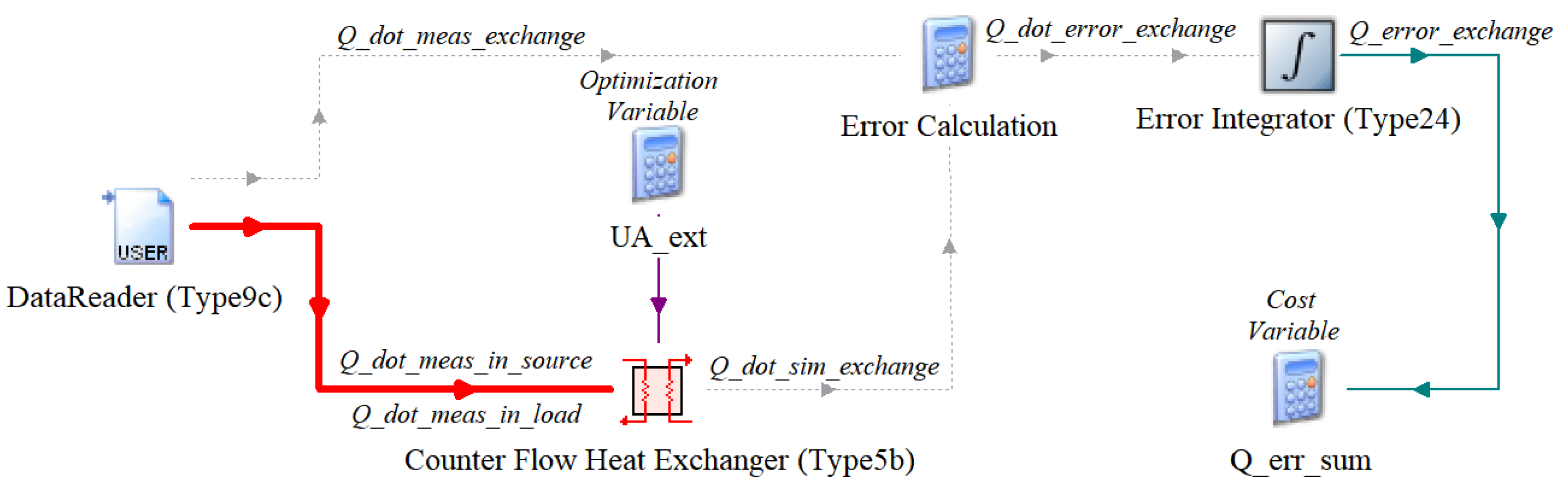
Figure 2.
Considered optimizer modes.
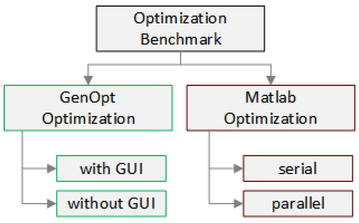
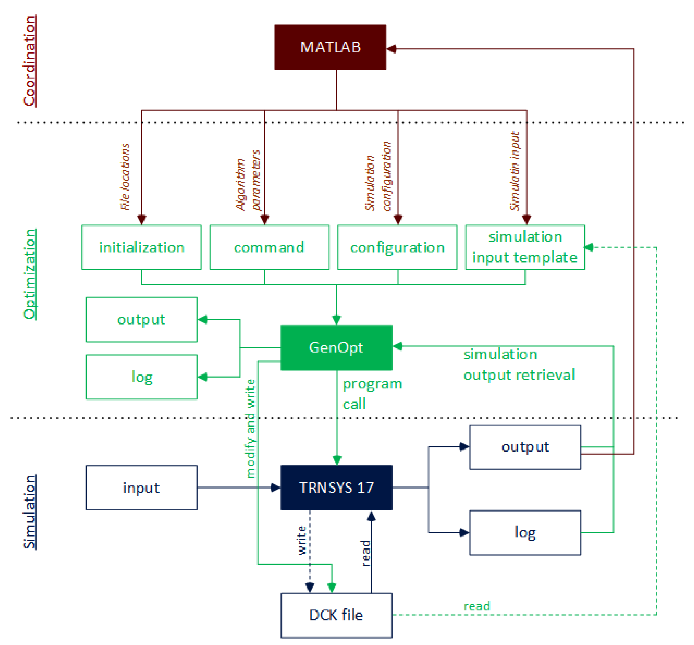
Figure 4.
Flow chart of coordinated optimization through GenOpt by MATLAB.
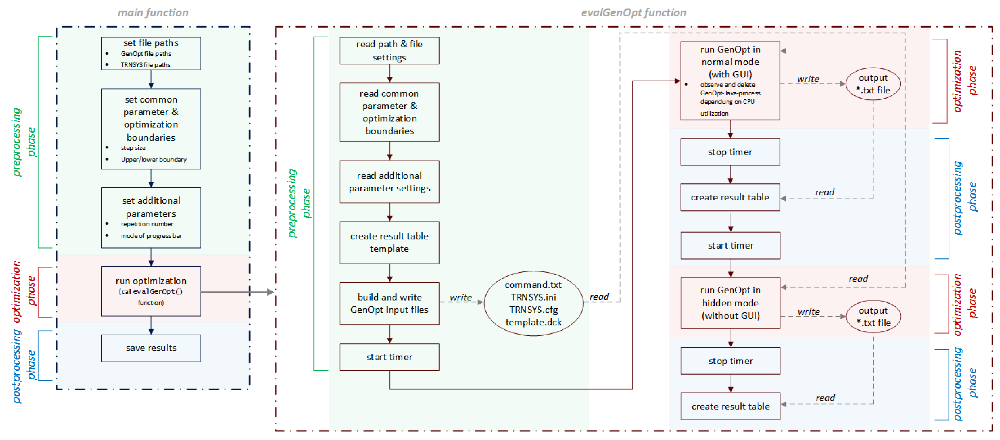
Figure 5.
Tool coupling of MATLAB and TRNSYS [34].
Figure 5.
Tool coupling of MATLAB and TRNSYS [34].
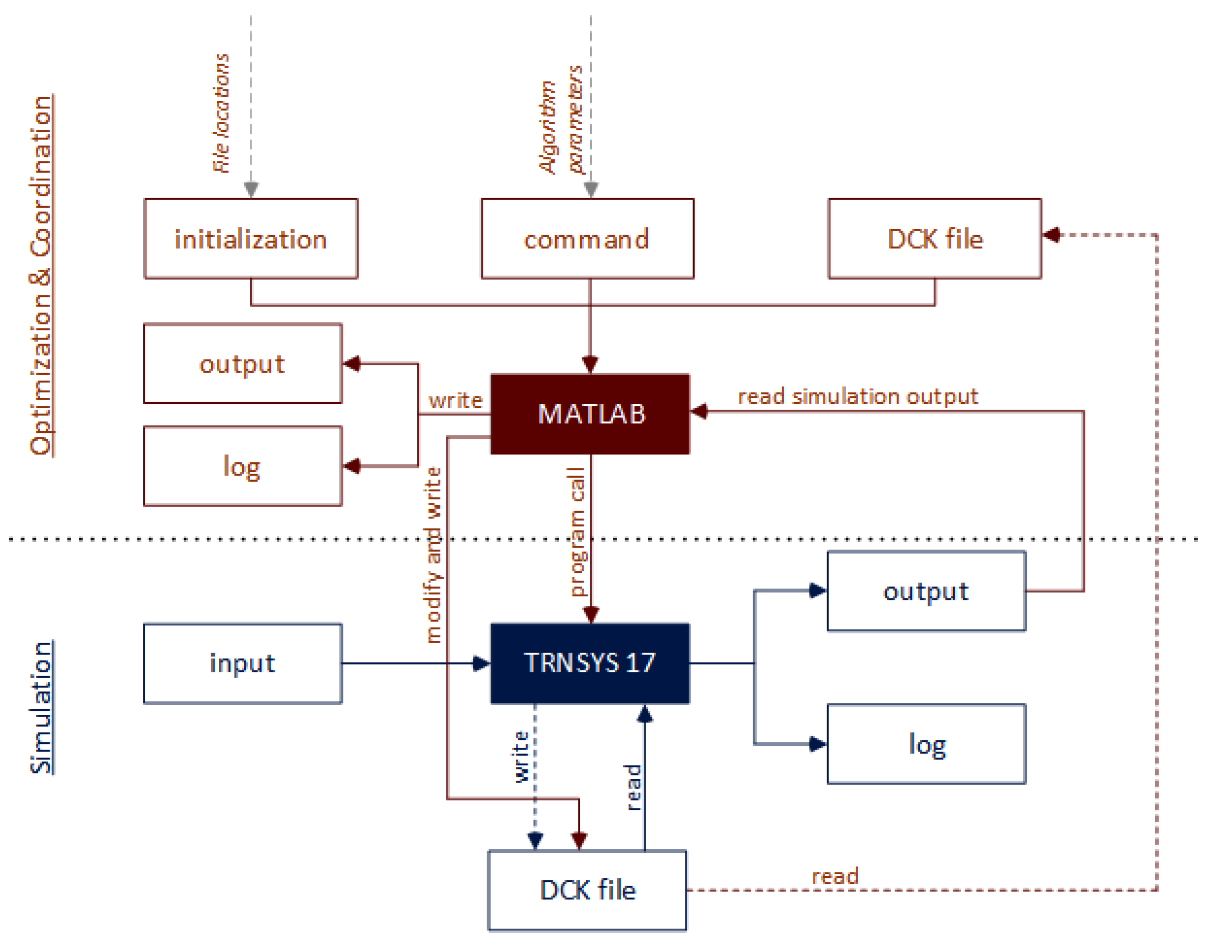
Figure 6.
Flow chart of optimization by MATLAB.
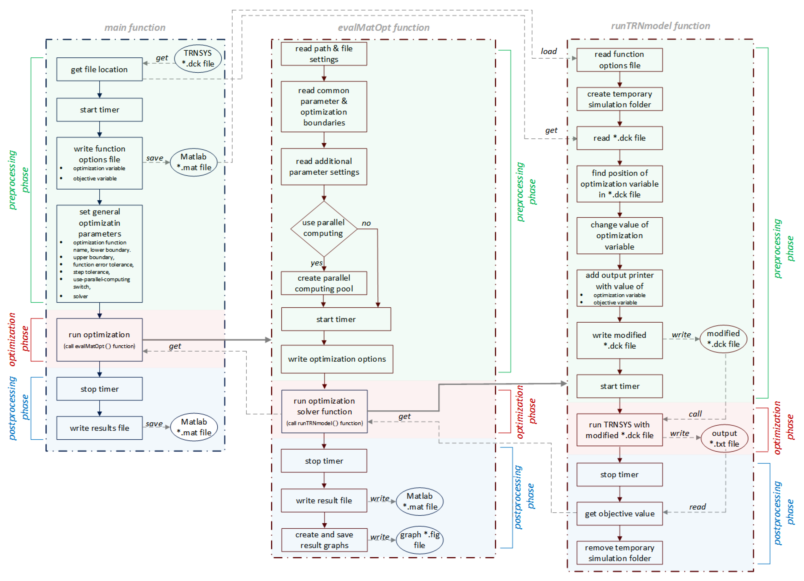
Figure 7.
GenOpt optimization results.
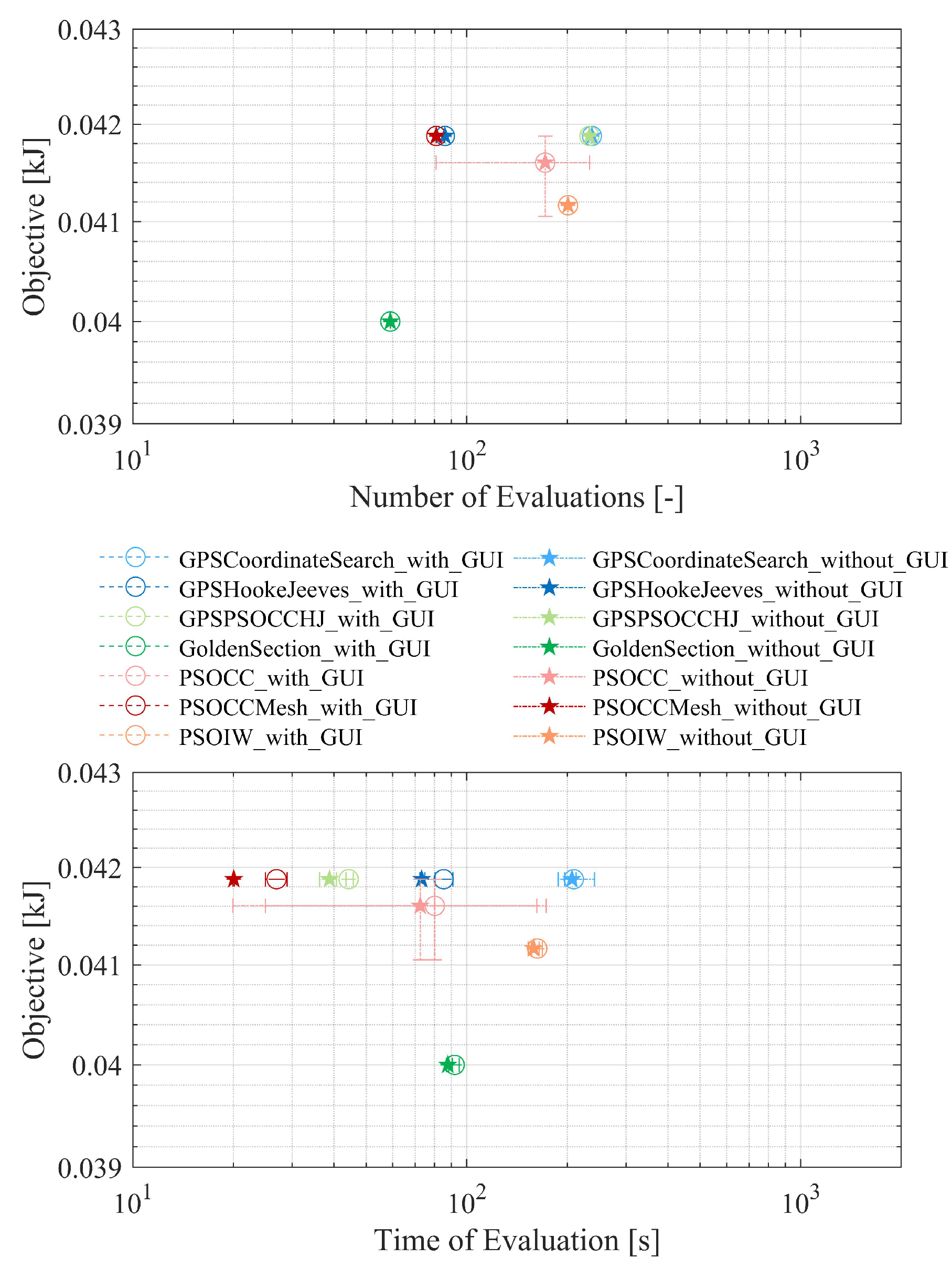
Figure 8.
MatOpt optimization results.
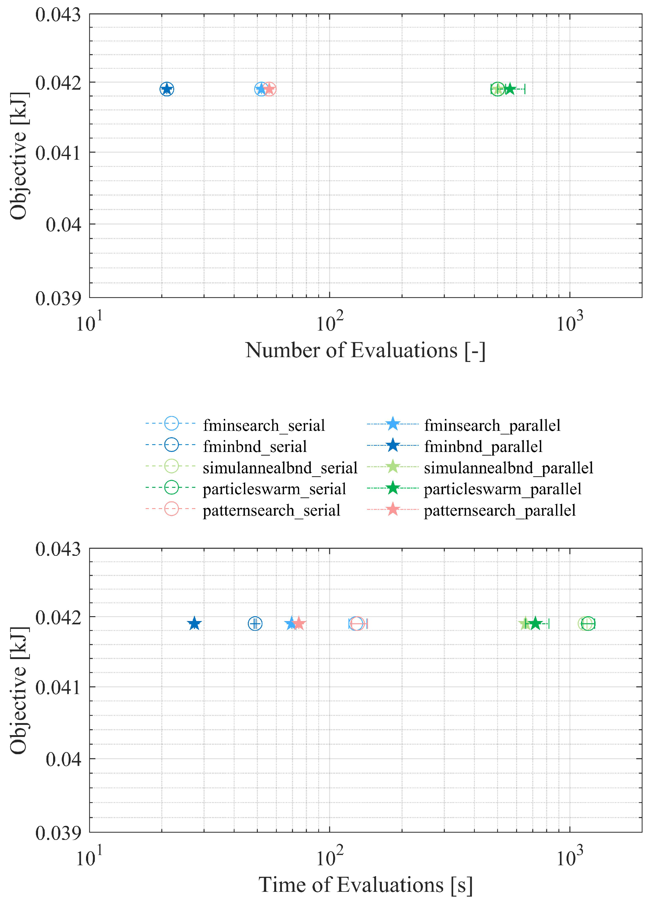
Table 2.
System Specification.
| System Parameters | Values |
|---|---|
| Processor | i5-3320M |
| Total Cores | 2 |
| Processor Clock Rate (GHz) | 2.6 |
| RAM (GB) | 16 |
| Type of Harddrive | SSD |
| Operating System | Windows 10 Pro |
| Architecture | x64 |
Table 3.
Common Solver Boundaries.
| Solver Parameters | Values |
|---|---|
| Lower boundary | 0 |
| Upper boundary | 5000 |
| Initial startpoint | 2500 |
| Maximum iteration steps | 500 |
Disclaimer/Publisher’s Note: The statements, opinions and data contained in all publications are solely those of the individual author(s) and contributor(s) and not of MDPI and/or the editor(s). MDPI and/or the editor(s) disclaim responsibility for any injury to people or property resulting from any ideas, methods, instructions or products referred to in the content. |
© 2024 by the authors. Licensee MDPI, Basel, Switzerland. This article is an open access article distributed under the terms and conditions of the Creative Commons Attribution (CC BY) license (http://creativecommons.org/licenses/by/4.0/).
Copyright: This open access article is published under a Creative Commons CC BY 4.0 license, which permit the free download, distribution, and reuse, provided that the author and preprint are cited in any reuse.


