
Submitted:
28 November 2024
Posted:
29 November 2024
You are already at the latest version
Abstract
In this paper, we consider a three-node free space optical (FSO) decode-and-forward (DF) cooperative network. The relay is not connected to a permanent power supply and relies solely on the optical energy harvested (EH) from the source node. This energy is accumulated in an energy buffer in order to enable the relay-destination communications. Moreover, buffer-aided (BA) relaying is considered where the relay is equipped with a data buffer for storing the incoming packets. For such networks, we propose a relaying protocol that delineates the roles of the source and the EH BA relay in each time slot. We develop a Markov chain framework for evaluating the analytical performance of the considered system. Numerical results validate the accuracy of the theoretical analysis and demonstrate significant reductions in the network outage, especially when the relay’s transmit level is appropriately selected.
Keywords:
Free Space Optics
; FSO
; relaying 3
; cooperative networks
; energy harvesting
; buffer-aided relaying
; buffer
; Markov chain
; performance analysis
; outage probability
1. Introduction
Relaying techniques are pivotal for wireless communications whether in the context of radio frequency (RF) or free space optical (FSO) networks. In RF systems, relaying techniques result in improved diversity orders by combatting the detrimental effects of fading that results from multi-path propagation. User coordination in dense environments is key for meeting the capacity demands in fifth generation systems where users participate in relaying, content delivery and computation within the network [1]. While FSO links are capable of carrying high-rate license-free optical signals, these links suffer from several atmospheric factors that limit the achievable performance levels. These include path loss, turbulence induced scintillation and pointing errors. In this context, relaying techniques were advised for FSO systems [2,3,4,5]. The work in [2] evaluated the diversity orders of decode-and-forward (DF) all-active and selective relaying techniques over gamma-gamma turbulence channels. The work in [3] considered the problem of relay placement for FSO multi-hop DF cooperative systems with link obstacles and infeasible regions. FSO relaying is also popular with unmanned-aerial-vehicle (UAV) communications where ground units with no direct line-of-sight communicate with each other through UAVs [4]. Recently, reinforcement learning was applied to solve the problem of relay selection and power allocation in FSO cooperative networks [5]. Many works in the open literature targeted mixed FSO/RF relaying systems as well. For example, [6] derived closed-form expressions of the end-to-end signal-to-noise ratio (SNR) in the case of a FSO satellite-to-relay link and a millimeter wave RF relay-to-user link.
Relaying strategies evolved from being buffer-free (BF) to becoming buffer-aided (BA) where the relays are equipped with data buffers (queues) for storing the received packets pending more convenient propagation conditions along the relay-destination hop [7,8,9]. Selecting a relay to either transmit or receive can be based on the channel state information (CSI) as in [7] where the strongest available link in the network is activated. Buffer state information (BSI) can also be included in the relay selection process resulting in reduced outage probabilities and queuing delays [8,9]. In this context, these algorithms privilege the reception and transmission at relays with small and large numbers of stored packets, respectively. While the FSO relaying systems in [2,3,4,5] are BF, BA FSO relaying was proposed and analyzed in [10,11] demonstrating improved diversity gains where a K-relay BA cooperative network will be in outage when all source-relay and relay-destination links suffer from outage. BA relaying was also considered with mixed and hybrid RF/FSO networks where the relay is equipped with a buffer for storing the packets from the mobile RF users before multiplexing the generated traffic over the backhaul FSO link [12,13,14].
Recently, there has been a surge of interest in energy harvesting (EH) solutions where the relays harvest RF and/or optical energy from the surrounding environment and/or from signals transmitted by other nodes in the network [15]. Such solutions enable relay-assisted communications even in the scenarios where the relays are not self-powered (i.e. not connected to a permanent power supply). EH also allows to prolong the battery lifetime in case batteries are available at the relay nodes. EH solutions include the well-known RF simultaneous wireless information and power transfer (SWIPT) technique [16] and the emerging simultaneous lightwave information and power transfer (SLIPT) method [17]. The SLIPT solution is very popular for indoor optical wireless communications (OWC) [18] in the context of sensor networks and Internet of Things (IoT) applications. The SLIPT technology was also investigated with outdoor OWC for ground-to-air, UAV-to-UAV and underwater communications [19]. The SLIPT technology revolves around separating the bias direct current (DC) and alternating current (AC) components from the received optical signal and using these components for information decoding and EH, respectively.
SLIPT has been studied extensively in the existing literature whether in the context of point-to-point communications [19,20,21] or relay-assisted communications [22,23,24,25,26,27]. The existing SLIPT relay-assisted communications are based on harvesting optical energy from the signal transmitted by the source through SLIPT along the first hop then directly using this energy to fuel the information transmission to the destination along the second hop that can be either a RF link [22,23,24,25,26] or an optical link [27]. In this context, the amount of harvested energy dictates the achievable performance levels along the relay-destination link that, in its turn, directly contributes to fixing the end-to-end performance that is limited by the weakest of the two hops. This constitutes a major limitation of the works in [22,23,24,25,26,27]. In fact, small levels of energy harvested in one time slot directly reflects to a performance loss over this slot while large amounts of harvested energy do not directly translate into performance improvements since the end-to-end performance might be dictated by the first hop (not the second hop). In order to overcome this limitation, the harvest-store-use (HSU) strategy was applied in [28] where the harvested energy is accumulated and stored in an energy buffer (battery or super-capacitor) to be further used to fuel the communications along the second hop. In this context, even if the energy harvested in one slot is small, the relay can rely on the previously stored energy to enable the communications along the second hop. While the HSU strategy was studied extensively in the context of RF communications [29,30], to the author’s best knowledge, [28] is the only reference that applied HSU with OWC using SLIPT.
On one hand, the existing BA FSO relaying techniques [10,11] assume self-powered relays that do not rely of EH. On the other hand, the existing non-HSU [22,23,24,25,26,27] and HSU [28] EH OWC relaying solutions overlook the possibility of equipping the relays with data buffers. As such, our work suggests closing this gap by investigating FSO BA relaying systems with an EH relay implementing the HSU strategy. This constitutes an additional degree of freedom where the relay is equipped with a data buffer and energy buffer for the sake of improving the performance of the DF cooperative network. To the author’s best knowledge, FSO relay-assisted systems were never studied before in the presence of these two types of buffers. As such, the contributions of this work are as follows:
- -
- Combining the BA and EH techniques in the context of a single-relay cooperative FSO network. The relay is equipped with a finite-size data buffer for storing the incoming packets from the source. It is also equipped with an infinite-size energy buffer to accumulate the energy harvested from the source through SLIPT. In the considered system model, the harvested energy is not dispensed on a slot-by-slot basis, but it is rather stored for future usage through the HSU methodology.
- -
- We carry out a theoretical evaluation of the considered FSO BA HSU system through a Markov chain analysis. This analysis revolves around discretizing the continuous-value energy buffer and deriving the state transition probabilities with the objective of evaluating the steady-state probability distributions of the data and energy buffers’ occupancies. These distributions are then used to derive the outage probability (OP) of the three-node FSO DF cooperative network.
- -
- The paper examines the effects of path loss, gamma-gamma atmospheric turbulence and pointing errors on the OP performance of the system. The presented numerical analysis validates the theoretical analysis highlighting the impacts of the target data rate, data buffer size, relay transmit level and relay position on the network OP.
2. System Model
2.1. Basic Parameters
Consider a three-node cooperative FSO network composed of a source (S), relay (R) and destination (D) as shown in Figure 1. S communicates with D either directly along the link S-D or indirectly through R along the two-hop path S-R-D. The relay R implements the DF protocol where the information packet received from S is decoded to be later retransmitted to D. In the considered system model, we assume that S is connected to a permanent power supply unlike R that relies solely on the optical energy harvested from S along the link S-R. The HSU methodology is implemented where R harvests optical energy from S, stores this energy in an energy buffer (battery or super-capacitor) and uses this energy to relay the information packets to D. In this context, S always has enough energy to communicate with D and R unlike R that can communicate with D only if it has sufficient amounts of energy stored in its energy buffer. We assume that the energy buffer has an infinite size which is a realistic assumption since the storing capabilities of modern batteries largely exceed the amounts of energy needed to transmit an information packet.
Unlike the previous work in [28] where the relaying protocol is implemented with a BF relay, we consider a BA relaying system where the relay is equipped with a data buffer (queue) of finite size L in which the information packets received from S can be stored before being retransmitted to D. This upgrade is critical for the EH relay whose stored energy levels might be insufficient and, hence, will resort to queuing the information packets pending the harvesting of more energy.
2.2. FSO Links
FSO links suffer from three major impairments. (i): The path loss (or attenuation) incurring a deterministic drop in the received power. (ii): Turbulence-induced scintillation that results from the random fluctuation of the index of refraction of air with the inhomogeneities in temperature and pressure variations. (iii): Misalignment-induced fading (pointing errors) where, in practice, the transmitting laser and receiving photodetector cannot be perfectly aligned given the continuous sway of the buildings on which the FSO transceivers are mounted. As such, the channel coefficient of the i-th link can be written as where denotes the path loss while captures the random variations of the channel coefficient resulting from scintillation and pointing errors with denoting the S-D link, denoting the S-R link and denoting the R-D link.
The path-loss term along link-i can be determined as follows [28,31]:
where , and stand for the attenuation coefficient, receiving area and diffraction-limited beam angle, respectively. From (1), the attenuation increases with the length of the i-th link where stands for the distance between S and D, stands for the distance between S and R and stands for the distance between R and D.
The turbulence-induced fading is often modeled by the gamma-gamma distribution that can capture a broad range of turbulence conditions. Assuming this model and a Gaussian spatial intensity profile falling on a circular aperture at the receiver, the probability density function (pdf) of the small-scale fading term was derived in [32]:
where is the Gamma function and is the Meijer G-function. In (2), and stand for the distance-dependent parameters of the gamma-gamma distribution:
where the Rytov variance is given by with k and denoting the wave number and refractive index structure parameter, respectively [31,32].
In (2), the parameters and are related to the pointing errors that depend on the radius of the i-th receiver, the pointing error displacement variance at the i-th receiver and the beam waist along the i-th link. Defining where stands for the error function, then and .
2.3. Information Transmission
Lasers operate under a peak power constraint where the transmitted power cannot exceed a certain maximum value denoted by . In this context, the modulated signals transmitted from S (to D and R) have an average power of where this value maximizes the lower bound on the channel capacity along the non-negative optical links operating under a peak power constraint [33].
An optical link is said to be in outage if the maximum data rate (or capacity) along this link falls below a certain target rate denoted by . As such, the outage probabilities and along the links S-D and S-R can be determined from:
where stands for the responsivity of the photo-detectors (in A/W) while stands for the variance of the additive white Gaussian noise (AWGN).
In FSO communications where FSO transceivers are usually mounted on buildings, power consumption is not a major issue at these transceivers that are connected to the power grid. Unlike S that is connected to a permanent power supply, energy consumption is a major challenge at R that relies completely on the harvested energy. As such, setting the average transmit power to at R will deplete its energy buffer at a fast pace rendering R incapable of transmitting packets to D. In other words, this energy shortage will render the R-D link unavailable. Moreover, this unavailability will imply that the data buffer at R will become congested since the incoming packets along the S-R link cannot be released along the R-D link. Therefore, the S-R link will become unavailable as well since the full data buffer at R cannot accommodate the incoming packets from S. Based on the above observations, we set the average power at R to where . Consequently, the outage probability of the R-D link is given by:
While setting penalizes the outage probability along the R-D link, this choice contributes to increasing the amount of energy stored in the energy buffer while concurrently decreasing the number of packets stored in the data buffer.
2.4. Energy Harvesting
The relay R harvests optical energy from the DC component of the light beam emitted by S through SLIPT. For solar-panel-based receivers, the harvested energy increases nonlinearly with the average transmitted power according to the relation [17]:
where f is the photo-detector’s fill factor, is the thermal voltage and stands for the dark saturation current. Since the scintillation coefficient is a random quantity, then the amount of energy harvested at R is random as well. In [28], the pdf of the harvested energy was derived as follows:
where is the pdf in (2), is the Lambert W-function, and .
2.5. Relaying Protocol
This section describes the proposed relaying protocol that takes into consideration the specificities of FSO communications as follows. (i): FSO links are highly directive following from the fact that laser beams are extremely narrow. The direct implication on the system design is that the two nodes S and R can transmit at the same time with no interference. (ii): FSO relays are full-duplex where the receiving optical unit at R (photodetector and demodulator) operates independently from the transmitting unit (laser and modulator). The implication of this particularity resides in the fact that R can concurrently transmit and receive with no interference. As a conclusion, for the considered FSO cooperative network, the three constituent links (S-D, S-R and R-D) can be activated simultaneously without interference.
Based on the above observation, the proposed energy-buffer-aided and data-buffer-aided relaying protocol operates as follows:
- -
- S simultaneously transmits an information packet to both D and R. In this step, S consumes a power of to transmit the packet to D along the S-D link (transceiver 1 to transceiver 5 in Figure 1) and the same amount of average power to transmit the same packet to R along the S-R link (transceiver 2 to transceiver 3 in Figure 1).
- -
-
Nodes D and R proceed as follows after the transmissions from S:
- -
- D attempts to decode the received packet and replies to S by an acknowledgement signal (ACK) if this attempt was successful and by a no-acknowledgement signal (NACK) otherwise.
- -
- R harvests energy from the DC component of the optical signal received from S and stores this energy in the energy buffer. Case 1: If D replied by an ACK, then S informs R not to decode the information packet since this packet has been successfully delivered to D. Case 2: If D replied by a NACK, then S notifies R to decode the information packet and store the reconstructed packet in its data buffer in case this buffer is not full. As such, R’s role is limited to EH in case 1 and to EH and information decoding in case 2.
- -
- Independently from the above steps, and following from the full-duplexity at R and the absence of interference in the system, R will always attempt to transmit an information packet (extracted from the data buffer) to D along the R-D link (transceiver 4 - transceiver 6 in Figure 1).
Therefore, the following conditions should be met for activating each one of the links in the network.
- -
- S-D link. (i): the channel should not be in outage with probability .
- -
- S-R link. (i): The S-D channel should be in outage. (ii): The S-R channel should not be in outage (with probability ). (iii): The data buffer at R should not be full so that the incoming packet can be accommodated.
- -
- R-D link. (i): The R-D channel should not be in outage (with probability ). (ii): The data buffer at R should not be empty so that an information packet can be extracted and sent to D. (iii): The amount of energy stored in the energy buffer should exceed the value of 1.
3. Performance Analysis
3.1. Preliminaries
A Markov chain analysis will be adopted for evaluating the performance of the proposed relaying system. The considered system is discrete in time where a time unit corresponds to the time spanned by the duration of one information packet. In this context, the role of each one of the three nodes is determined at the beginning of each time slot in a slot-by-slot basis. The data buffer occupancy assumes discrete values corresponding to the numbers of stored packets . On the other hand, the energy buffer content assumes continuous values . Since the analysis of a mixture of discrete-value and continuous-value processes is challenging, the energy levels e stored in the energy buffer will be discretized resulting in a discrete-time discrete-value Markov chain whose analysis is more tractable.
The discretization of the infinite-size energy buffer will be carried out in the following manner. The energy value of needed to transmit a packet from R will be considered to span M energy units of the energy buffer. As such, the energy interval will be divided into M intervals of size each. As such, the energy interval of the energy buffer will be mapped to the energy intervals:
with being a sufficiently large number in order to span the full range of the infinite-size energy buffer in an accurate manner. As will be highlighted later, the amounts of harvested energy are usually small implying that it is not probable to have significantly large amounts of energy stored in the energy buffer. As such, does not need to assume prohibitively large values in order to fully describe the dynamics of the infinite-size energy buffer.
Therefore, the relaying system will be described by a discrete-time discrete-value Markov chain whose state space comprises states as follows:
where the state denotes that l packets are stored in the data buffer and the energy stored in the energy buffer falls in the interval for and in the interval for .
We define as the probability that the harvested energy moves the discretized energy buffer from the energy state m to the energy state with . This probability can be evaluated as follows:
where is the pdf of the harvested energy given in (8).
Equation (11) can be further simplified as follows:
where is the cumulative distribution function (cdf) of the harvested energy that can be determined from ():
The probabilities in (12) satisfy the two following relations:
where the proofs of these two relations are provided in Appendix A.
A main challenge in the Markov chain analysis resides in the fact that the value of the random variable defines the amount of energy harvested at R (from (7)) and also determines whether the S-R channel is in outage or not (from (5) for ). As such, the harvested energy and S-R outage events are not independent and the outage probability cannot appear explicitly in the description of the Markov chain. From (5), the S-R channel is in outage if falls below the following threshold value:
Since the harvested energy in (7) is an increasing function of , then replacing (16) in (7) implies that the S-R channel would be in outage if the harvested energy falls below the following threshold value:
where is constant for a given value of .
Following from the discretization of the energy buffer, we define the integer as follows:
Therefore, according to the proposed formulation, the transition from the energy state m to the energy state with implies that the harvested energy is smaller than and the channel coefficient is smaller than implying that the S-R link is in outage.
As a conclusion, the dynamics of the Markov process will depend on the four integers L, M, and . Note that M should be large enough for a fine discretization of the energy buffer and should be very large since the energy buffer has an infinite size. Since and , then since the harvested energy is several orders of magnitude smaller than the energy needed to transmit an information packet.
3.2. Transition Probabilities
After discretizing the energy buffer and defining the states of the Markov chain, this section covers the transition probabilities among all states of the state space. We define as the probability of going form state to the state for all values of and . The probabilities of all transitions leaving any state should add up to one implying that the following relation must hold:
We derive the transition probabilities in the two cases and .
3.2.1. Case I:
In this case, R does not have enough energy to transmit. As such, the number of packets stored in the data buffer can either remain the same or increase by one implying that for . Similarly, since R harvests energy from the optical signal transmitted by S during any time slot while no energy is dispensed since R cannot transmit, then the energy stored in the energy buffer cannot decrease implying that:
In what follows, we derive the transition probabilities when .
Case I.1: For , R cannot receive a packet from S since the data buffer is full. This holds regardless of statuses of the S-D and S-R channels. Therefore, the content of the data buffer remains the same (since R cannot transmit or receive in this case) while the harvested energy will move the energy buffer from the energy state m to the energy state (with ). Therefore:
Case I.2: Consider now the case . In this case, R can receive a packet from S (while it is not possible for R to transmit to D). For , if , then the S-R channel is in outage and a packet cannot be delivered from S to R implying that the occupancy of the data buffer remains unchanged. Consequently:
On the other hand, if , then the S-R channel is not in outage and R can successfully decode the packet transmitted from S. Following from the relaying protocol in Section 2.5:
since, when the S-D link is not in outage (with probability ), R will not decode and store the incoming packet implying that the data buffer occupancy with remain the same. On the other hand, if the S-D link is in outage (with probability ), then the number of packets stored in the data buffer will increase by one since R will decode and store the packet that was not delivered to D.
3.2.2. Case II:
In this case, R has enough energy to transmit. As such, R will proceed with transmitting a packet to D only if the data buffer is not empty and the R-D channel is not in outage.
Case II.1: Consider the case . In this case, the data buffer is empty implying that the R-D link is not available for data communications. As such, the transition probabilities are similar to those derived in (20), (22) and (23) in case I.2 since R might or might not receive while it cannot transmit. These probabilities are restated below for easy referencing:
Case II.2: Consider the case where the data buffer (that is neither empty nor full) does not hinder any of the S-R or R-D transmissions where both types of transmission might be triggered. As such , the data buffer state can evolve from the initial state l to the three possible final states .
Consider first the case . In this case, R has transmitted a packet but it did not receive any packet. Since R has successfully transmitted a packet, then the R-D channel is not in outage with probability . Moreover, R has dispensed an energy of for transmitting the packet implying that the state of the energy buffer will drop by M units from the state m to the state . Therefore:
since the stored energy cannot drop by more than M units. On the other hand, the S-R link was not activated despite the fact that the data buffer is not full implying that either the S-D channel is not in outage or both the S-D and S-R channels are in outage.
For , then the transition of the energy buffer can be divided into the following two transitions where the first transition results from the reduction in energy resulting from the transmission from R while the second transition corresponds to the increase in energy resulting from energy harvesting. If , then the small amount of harvested energy implies that the S-R channel is in outage implying that no packet will be delivered to R regardless of the status of the S-D link. Consequently, for and :
On the other hand, for , then the S-R channel is not in outage implying that the only reason for R not to receive a packet is that the S-D channel is not in outage (with probability ) implying that the packet was delivered directly to D. Therefore:
Consider next the case . In this case, R has received a packet but it did not transmit any packet. The only reason for R not to transmit is the outage of the R-D channel (with probability ) since the data buffer is not empty and the energy buffer contains enough stored energy. Since R did not transmit, then the stored energy cannot decrease implying that:
On the other hand, for and , then the transition is improbable since the relation implies that the S-R channel is in outage while the increase in the number of stored packets cannot take place unless this channel is not in outage. Therefore:
For :
since R has received a packet which cannot happen unless when the S-D channel is in outage with probability .
Finally, consider the case . In this case, the full-duplex relay has either concurrently transmitted and received or it did not neither transmit nor receive. In both cases, the content of the energy buffer cannot drop by more than M units implying that:
Consider now the case and . The last relation implies that the S-R channel is in outage and, as such, R cannot receive. Since the number of packets stored at R did not change, then this implies that R did not transmit which is not possible since the energy stored in the energy buffer decreased ( since ). Therefore, the transition is not possible in this scenario:
For and , then the drop of energy in the energy buffer means that R has transmitted implying that it has received as well sp that the number of stored packets remained unchanged. Since R can successfully transmit only if the R-D channel is not in outage while R can receive only if the direct link S-D is in outage, then:
For and , then the two following cases are possible. (i): The increase in the stored energy took place solely because of EH where R did not transmit and did not receive. (ii): R has transmitted dispensing M energy units but had harvested more energy than it had dispensed implying the two transitions . Since R has transmitted in this case, then it should have definitely received since the content of the data buffer remained unchanged. Therefore:
In the last equation, was multiplied by since R did not transmit implying that the R-D channel is in outage while the relation implies that the S-R channel is in outage as well. On the other hand, was multiplied by since R has transmitted and received implying that the R-D channel is not in outage and the direct S-D channel is in outage since, otherwise, the packet would have been communicated directly and not relayed to R. Note that in this case, the S-R channel is not in outage since:
since .
Finally, consider the case and where last relation implies that the S-R channel is not in outage. In this case, (39) should be amended as follows:
where was multiplied by the additional term since, in this case where the S-R channel is not in outage, the only reason for R not to receive is the availability of the direct S-D link.
The transition probabilities pertaining to Case II.2 (where R has enough energy to transmit and the data buffer is neither full nor empty) are shown in Figure 2. In Appendix B, we prove that the transition probabilities in (31), (32), (35), (38), (39) and (41) satisfy the relation in (19).
Case II.3: Consider the case where the data buffer is full and R cannot receive regardless of the statuses of the S-D and S-R channels. As such, R only harvests energy along the S-R link.
The successful transmission from R implies the following transitions:
where the first relation follows since the drop in the stored energy cannot exceed M units because of EH. The second relation results from the two following energy buffer transitions where the first transition results from consuming energy for R to transmit while the second transition results from EH. In this case, should be multiplied by since the R-D channel should not be in outage for R to be able to transmit.
On the other hand, the unsuccessful transmission from R (because of the outage of the R-D channel) implies the following transitions:
3.3. State Transition Matrix
The state transition matrix is a matrix that describes all transitions between the states of the Markov chain. For the considered Markov chain, assumes the following block structure:
where is the all-zero matrix and are matrices describing the transitions from the data buffer state l to state for . In this context, the -th element of matrix is equal to for . Following from (19), the sum of each column of should be equal to 1.
3.3.1. Matrices and
From equations (22), (23), (28) and (29), matrix is a lower-triangular Toeplitz matrix that can be constructed as follows:
3.3.2. Matrices and
Following from (42) and from the fact that R does not have enough energy to transmit when (i.e. for ), then matrix can be constructed as follows:
where for . Note that elements of the first M columns of are equal to zero.
3.3.3. Matrices , and for
Since (22) and (23) do not depend on the specific value of l for and , then the first M columns of the matrix are equal to the first M columns of the matrix in (45). Regarding the last columns of , these can be generated by adding the first columns of (from (46)) with the first columns of the Toeplitz matrix generated from the following vector:
where the above relation follows from (39) and (41).
Finally, note that the relation in (14) was applied for constructing the matrices reported in this section justifying why the first subscript of the probabilities is always equal to zero.
3.4. Steady-State Distribution and Outage Probability
The transition matrix is used to evaluate the steady-state probability distribution vector [7,34,35]:
where and are matrices denoting the identity matrix and all-one matrix, respectively. Vector is the -dimensional vector whose elements are all equal to 1.
Vector is a vector that can be written as:
where stands for the probability that the data buffer contains l packets and the energy buffer comprises m units of energy when the Markov chain reaches steady-state.
Deriving the steady-state distribution from (52) is key for evaluating the outage performance of the cooperative network. The network is said to be in outage if no packets can be communicated along its three S-D, S-R and R-D constituent hops. The outage probability can be evaluated as follows:
where stands for the probability that the S-D, S-R and R-D links are unavailable when the Markov chain is in state .
For , the R-D link is unavailable since no packets can be extracted from the data buffer to be communicated to D. As such, the network will be in outage whenever the S-D and S-R links would be in outage implying that:
For , the state of the data buffer does not hinder the S-R and R-D communications. (i): For , R does not have enough energy to transmit rendering the R-D link unavailable. In this case, the network will be in outage if the S-D and S-R links are in outage. (ii): For , R can transmit implying that the concurrent outages of the S-D, S-R and R-D channels will hinder the flow of packets in the network. Therefore:
For , the S-R link is unavailable since a full data buffer cannot accommodate an incoming packet. Therefore, the network will be in outage if the S-D channel is in outage and the R-D link is unavailable (either because of insufficient amounts of stored energy or because of channel outage). Therefore:
4. Numerical Results
We next present some numerical results that support the theoretical findings reported in the previous section. The numerical results are generated based on Monte Carlo simulations where 1000 epochs were considered each covering the transmission of packets. For each epoch, the continuous value of the energy stored in the energy buffer and the discrete value of the number of packets stored in the data buffer were updated based on the relaying strategy in Section 2.5 and the arising network outage events were counted and averaged. The theoretical results are based on the Markov chain analysis where the OP is derived from (54) using the steady-state distribution obtained from (52). We fix and where these values were sufficient for generating accurate results.
We consider the two following scenarios. Scenario 1 where the S-R and R-D distances are fixed to km and km, respectively. Scenario 2 with km and km. For both scenarios, the distance between S and D is fixed to km. The simulations are performed under “clear air” weather conditions where all simulation parameters are provided in Table 1. We assume that the receivers’ parameters are the same for all nodes and that the weather conditions are the same along all optical links. As a benchmark, we show the OP of direct point-to-point communications along the S-D link with no cooperation where the OP is equal to . We also show the performance of the buffer-free (BF) relaying system in the case where R is connected to a permanent power supply; in this case, the OP is given by . Note that the OPs of the direct and BF communications do not change under the two considered simulation scenarios since is fixed while and (and, as such, and ) are interchanged in the two scenarios.
Figure 3 shows the OP variations with the threshold rate under the two simulation scenarios with the data buffer size fixed to and the power factor assuming the values of 0.75 and 1. Results in Figure 3 show that the proposed BA relaying scheme outperforms direct communications for all values of under the two scenarios. In this context, the performance gains are more pronounced for smaller values of . Moreover, the OP values are smaller for scenario 1 since R is closer to S and, hence, can harvest larger amounts of energy that eventually contribute to an improved availability of the R-D link. Figure 3 demonstrates the significant impact of on the performance. While larger values of result in reduced values of , such reduction does not necessarily translate into improved performance since R consumes more energy when it transmits implying that it has to wait for much more time to harvest and store the energy needed for this transmission. On the other hand, smaller values of make a better use of the energy stored in the energy buffer, hence, avoiding the depletion of this buffer at a fast pace and boosting the availability of the R-D link. Finally, results in Figure 3 highlight the extremely close match between the numerical and theoretical results, thus, demonstrating the accuracy of the performed Markov chain analysis.
For the simulation setup of Figure 3, the steady-state distribution of the data buffer content is shown in Figure 4 for bit/s/Hz. This figure reports the probability distribution of having l packets stored in the data buffer for . For the numerical results, this distribution was obtained by counting the number of stored packets in all iterations of all epochs. For the theoretical Markov chain analysis, this distribution can be determined from the steady-state distribution in (52)-(53) using the relation . Results in Figure 4 demonstrate the accuracy of the theoretical distribution that perfectly matches the numerical distribution. For , results show that the data buffer is congested where is very small for . In fact, the high power consumption at R implies that R will not have enough energy to transmit the incoming packets incurring the queuing of these packets in the data buffer until a sufficient amount of harvested energy is accumulated. On the other hand, for , the probability distribution is spread among a broader range of values of l and the probability of having a full data buffer decreases compared to the case . For example, for scenario 1 (resp. scenario 2), decreases from to (resp. from to ) as decreases from 1 to 0.75. In this context, it’s worth reiterating that a full data buffer renders R incapable of receiving packets from S since there is no space to store these packets.
In order to study the impact of the power factor on the performance, Figure 5 shows the variations of the OP as a function of for and bit/s/Hz. The OP along the direct S-D link does not depend on . For the buffer-free system with a self-powered relay, we fixed to its best value of 1 that minimizes the value of and, consequently, minimizes the resulting OP. Note that power consumption is not problematic at the self-powered relay and can be set to its maximum value of 1. As in the previous figures, results in Figure 5 demonstrate the close match between the numerical and theoretical results. For scenario 1 that profits from more pronounced EH levels, all values of up to 0.4 result in approximately the same advantageously small OP value of around . Beyond , the OP increases rapidly reflecting a starvation of the energy buffer resulting from the excessive amounts of energy allocated for transmitting packets. For scenario 2 where the EH levels are limited, the best OP performance of around is obtained for . The following findings can be drawn from Figure 5. (i): The proposed scheme is capable of reducing the OP compared to direct communications for all values of . (ii): Decreasing to very small values is not useful. Even though this reduction saves energy at R; however, this extreme reduction severely compromises the quality of communications along the R-D link rendering this link unavailable. In other words, R will be saving energy, but it will not make good use of this energy to deliver the packets to D. (iii): The proposed scheme relying solely on the harvested energy has the potential of outperforming the buffer-free systems with self-powered relays. While the EH relaying scheme significantly outperforms buffer-free systems for in scenario 1, comparable OPs are observed for under scenario 2 where R is farther from S.
While the data buffer size was fixed to in Figure 3, Figure 4 and Figure 5, the simulations in Figure 6 show the impact of L on the OP for bit/s/Hz. Results show that the size of the data buffer does not have a visible impact on the performance where the OP is almost constant under scenario 1 and scenario 2 for the considered values of . As such, the energy buffer (and not the data buffer) constitutes the bottleneck of the EH relaying system and a small data buffer size is sufficient for extracting the full capabilities of BA relaying.
Figure 7 highlights the impact of the relay’s position on the OP for . We fix the S-D distance to km and vary the position of R along the line joining S to D. As such, we plot the OP as a function of the variable distance between S and R where and km. For the two considered values of (bits/s/Hz), results show the OP reductions that result from reducing from 1 to 0.6. While the performance of buffer-free systems with a self-powered relay is optimized when the relay is placed at the center between S and D (i.e. km) in coherence with the well established results in the literature, Figure 7 shows that it is best to place R as close as possible to S with an EH relay. Evidently, this option increases the amounts of energy that can be harvested at the relay. Moreover, the shortcoming of compromising the quality of the R-D communications is not very critical since R does not always have enough energy to transmit.
5. Conclusions
This work highlighted the benefit of taking advantage from the presence of neighboring nodes to serve as relays, even when these relays would rely solely on the free energy harvested from the source node. Equipping the relay with a data buffer adds a new degree of freedom to the system design, allowing the relay to store the incoming packets until sufficient amounts of energy are accumulated in the energy buffer. Controlling the relay’s transmit energy turned out to be of paramount importance for improving the outage performance making a better use of the scarce energy harvested at the relay. We presented a Markov chain analysis to capture the dynamics of the data and energy buffers. This analysis culminated in evaluating the analytical outage probability of the cooperative network with the FSO links suffering from path loss, scintillation and pointing errors. Future works will consider extending the considered single-relay system to multi-relay scenarios.
Funding
This research was supported by the Lebanese American University.
Institutional Review Board Statement
Not Applicable.
Informed Consent Statement
Not Applicable.
Data Availability Statement
Not Applicable.
Conflicts of Interest
The authors declare no conflicts of interest.
Appendix A
The relation in (14) follows directly from (12) where it can be observed that, for , depends on and not on the particular value of m. The rationale behind this property is that the harvested energy is related to the difference between the energies of the discretized energy states.
Now, consider the summation in (15). For , this summation is equal to from (11) implying that this summation is equal to 1 since is a pdf defined for .
For :
Appendix B
Form (31):
| 1 | The time unit is normalized to unity. As such, the terms energy and power will be used interchangeably in the sequel. |
References
- M. Agiwal, A. Roy, and N. Saxena, “Next generation 5G wireless networks: A comprehensive survey,” IEEE communications surveys & tutorials, vol. 18, no. 3, pp. 1617–1655, 3rd Quarter 2016. [CrossRef]
- C. Abou-Rjeily, “Performance analysis of FSO communications with diversity methods: Add more relays or more apertures?” IEEE J. Select. Areas Commun., vol. 33, no. 9, pp. 1890 – 1902, Sep. 2015.
- B. Zhu, J. Cheng, M. Alouini, and L. Wu, “Relay placement for FSO multi-hop DF systems with link obstacles and infeasible regions,” IEEE Trans. Wireless Commun., vol. 14, no. 9, pp. 5240 – 5250, Sep. 2015.
- P. Li, X. Wei, X. Tang, J. Deng, and J. Xu, “UAV-assisted free space optical communication system with decode-and-forward relaying,” IEEE Trans. Veh. Technol., 2024, accepted for publication. [CrossRef]
- S. Xie and Y. Han, “Joint relay selection and power allocation in free-space optical communication with reinforcement learning,” in 2023 5th In. Academic Exchange Conf. on Science and Technology Innovation (IAECST). IEEE, 2023, pp. 313–317.
- Q. Sun, Q. Hu, Y. Wu, X. Chen, J. Zhang, and M. López-Benítez, “Performance analysis of mixed FSO/RF system for satellite-terrestrial relay network,” IEEE Trans. Veh. Technol., 2024, accepted for publication. [CrossRef]
- I. Krikidis, T. Charalambous, and J. S. Thompson, “Buffer-aided relay selection for cooperative diversity systems without delay constraints,” IEEE Trans. Wireless Commun., vol. 11, no. 5, pp. 1957–1967, May 2012. [CrossRef]
- S. El-Zahr and C. Abou-Rjeily, “Threshold based relay selection for buffer-aided cooperative relaying systems,” IEEE Trans. Wireless Commun., vol. 2, no. 9, pp. 6210–6223, Sep. 2021. [CrossRef]
- P. Xu, J. Quan, G. Chen, Z. Yang, Y. Li, and I. Krikidis, “A novel link selection in coordinated direct and buffer-aided relay transmission,” IEEE Trans. Wireless Commun., vol. 22, no. 5, pp. 3296–3309, May 2023. [CrossRef]
- C. Abou-Rjeily and W. Fawaz, “Buffer-aided relaying protocols for cooperative FSO communications,” IEEE Trans. Wireless Commun., vol. 16, no. 12, pp. 8205–8219, Dec. 2017. 10.1109/twc.2017.2759107.
- C. Abou-Rjeily, “Improved buffer-aided selective relaying for free space optical cooperative communications,” IEEE Transactions on Wireless Communications, vol. 21, no. 9, pp. 6877–6889, Sep. 2022. [CrossRef]
- V. Jamali, D. S. Michalopoulos, M. Uysal, and R. Schober, “Link allocation for multiuser systems with hybrid RF/FSO backhaul: Delay-limited and delay-tolerant designs,” IEEE Trans. Wireless Commun., vol. 15, no. 5, pp. 3281–3295, May 2016. [CrossRef]
- Y. F. Al-Eryani, A. M. Salhab, S. A. Zummo, and M.-S. Alouini, “Protocol design and performance analysis of multiuser mixed RF and hybrid FSO/RF relaying with buffers,” OSA J. Opt. Commun. Netw., vol. 10, no. 4, pp. 309–321, Apr. 2018. [CrossRef]
- C. Abou-Rjeily, “Packet unloading strategies for buffer-aided multiuser mixed RF/FSO relaying,” vol. 9, no. 7, pp. 1051–1055, July 2020. [CrossRef]
- S. Bi, Y. Zeng, and R. Zhang, “Wireless powered communication networks: An overview,” IEEE Wireless Commun., vol. 23, no. 2, pp. 10–18, Apr. 2016. [CrossRef]
- X. Zhou, R. Zhang, and C. K. Ho, “Wireless information and power transfer: Architecture design and rate-energy tradeoff,” IEEE Trans. Commun., vol. 61, no. 11, pp. 4754–4767, Nov. 2013.
- P. D. Diamantoulakis, G. K. Karagiannidis, and Z. Ding, “Simultaneous lightwave information and power transfer (SLIPT),” IEEE Trans. on Green Commun. and Networ., vol. 2, no. 3, pp. 764–773, Sep. 2018. [CrossRef]
- G. Pan, P. D. Diamantoulakis, Z. Ma, Z. Ding, and G. K. Karagiannidis, “Simultaneous lightwave information and power transfer: Policies, techniques, and future directions,” IEEE Access, vol. 7, pp. 28 250–28 257, Mar. 2019.
- C. Abou-Rjeily, G. Kaddoum, and G. K. Karagiannidis, “Ground-to-air FSO communications: when high data rate communication meets efficient energy harvesting with simple designs,” OSA Optics Express, vol. 27, no. 23, pp. 34 079–34 092, Nov. 2019. [CrossRef]
- H.-V. Tran, G. Kaddoum, P. D. Diamantoulakis, C. Abou-Rjeily, and G. K. Karagiannidis, “Ultra-small cell networks with collaborative RF and lightwave power transfer,” IEEE Trans. Commun., vol. 67, no. 9, pp. 6243–6255, Sep. 2019. [CrossRef]
- N. Shanin, H. Ajam, V. K. Papanikolaou, L. Cottatellucci, and R. Schober, “Accurate EH modelling and achievable information rate for SLIPT systems with multi-junction photovoltaic receivers,” IEEE Trans. Commun., 2024, accepted for publication. [CrossRef]
- H. Peng, Q. Li, A. Pandharipande, X. Ge, and J. Zhang, “End-to-end performance optimization of a dual-hop hybrid VLC/RF IoT system based on SLIPT,” IEEE Internet of Things Journal, vol. 8, no. 24, pp. 17 356–17 371, Dec. 2021. [CrossRef]
- S. Huang, G. Chuai, W. Gao, and K. Zhang, “Agency selling format-based incentive scheme in cooperative hybrid VLC/RF IoT system with SLIPT,” IEEE Internet of Things Journal, vol. 10, no. 8, pp. 7366–7379, April 2022. [CrossRef]
- D. AlQahtani, Y. Chen, and W. Feng, “Practical non-linear responsivity model and outage analysis for SLIPT/RF networks,” IEEE Transactions on Vehicular Technology, vol. 70, no. 7, pp. 6778–6787, July 2021. [CrossRef]
- A. Girdher, A. Bansal, and A. Dubey, “Analyzing SLIPT for DF based mixed FSO-RF communication system,” in 2021 28th Int. Conf. on Telecommun. (ICT). IEEE, 2021, pp. 1–7.
- Y. Xiao, P. D. Diamantoulakis, Z. Fang, L. Hao, Z. Ma, and G. K. Karagiannidis, “Cooperative hybrid VLC/RF systems with SLIPT,” vol. 69, no. 4, April 2021, pp. 2532–2545. [CrossRef]
- C. Álvarez-Roa, M. Álvarez-Roa, F. J. Martín-Vega, M. Castillo-Vázquez, T. Raddo, and A. Jurado-Navas, “Performance analysis of a vertical FSO link with energy harvesting strategy,” vol. 22, no. 15. MDPI, 2022, p. 5684. [CrossRef]
- C. Abou-Rjeily and G. Kaddoum, “Free space optical cooperative communications via an energy harvesting harvest-store-use relay,” IEEE Trans. Wireless Commun., vol. 19, no. 10, pp. 6564–6577, Oct. 2020. [CrossRef]
- D. Bapatla and S. Prakriya, “Performance of energy-buffer aided incremental relaying in cooperative networks,” IEEE Trans. Wireless Commun., vol. 18, no. 7, pp. 3583–3598, July 2019. [CrossRef]
- ——, “Performance of a cooperative network with an energy buffer-aided relay,” IEEE Trans. on Green Commun. and Networ., vol. 3, no. 3, pp. 774–788, Sep. 2019.
- B. Zhu, J. Cheng, and L. Wu, “A distance-dependent free-space optical cooperative communication system,” IEEE Commun. Lett., vol. 19, no. 6, pp. 969–972, June 2015. [CrossRef]
- H. Sandalidis, T. Tsiftsis, and G. Karagiannidis, “Optical wireless communications with heterodyne detection over turbulence channels with pointing errors,” J. Lightwave Technol., vol. 27, no. 20, pp. 4440–4445, October 2009. [CrossRef]
- A. Lapidoth, S. M. Moser, and M. A. Wigger, “On the capacity of free-space optical intensity channels,” IEEE Trans. Inform. Theory, vol. 55, no. 10, pp. 4449–4461, Oct. 2009.
- S. Luo and K. C. Teh, “Buffer state based relay selection for buffer-aided cooperative relaying systems,” IEEE Trans. Wireless Commun., vol. 14, no. 10, pp. 5430–5439, Oct. 2015. [CrossRef]
- Z. Tian, Y. Gong, G. Chen, and J. Chambers, “Buffer-aided relay selection with reduced packet delay in cooperative networks,” IEEE Trans. Veh. Technol., vol. 66, no. 3, pp. 2567–2575, Mar. 2017. [CrossRef]
Figure 1.
Buffer-aided FSO relaying with an energy harvesting relay.
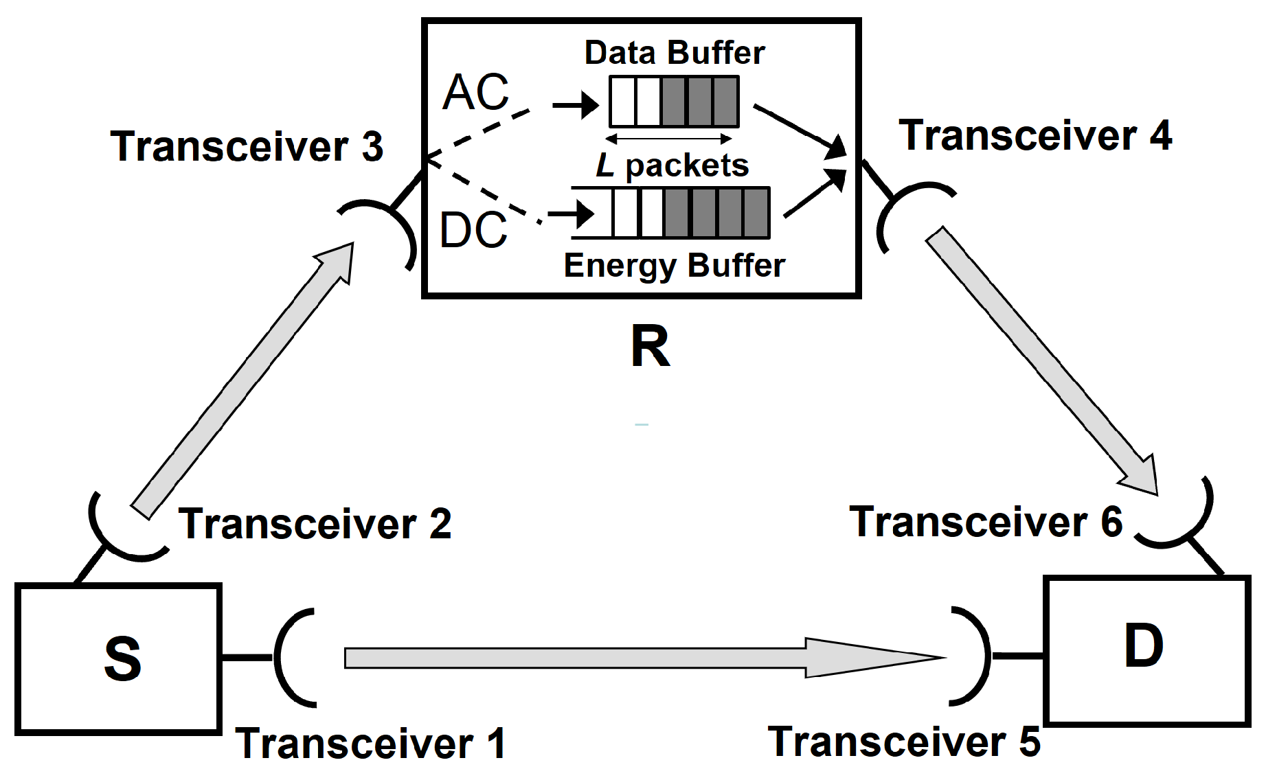
Figure 2.
Transition probabilities when the energy buffer has enough stored energy and the data buffer is neither full nor empty. The probabilities , , , , and correspond to the transition probabilities in equations (31), (32), (35), (38), (39) and (41), respectively.
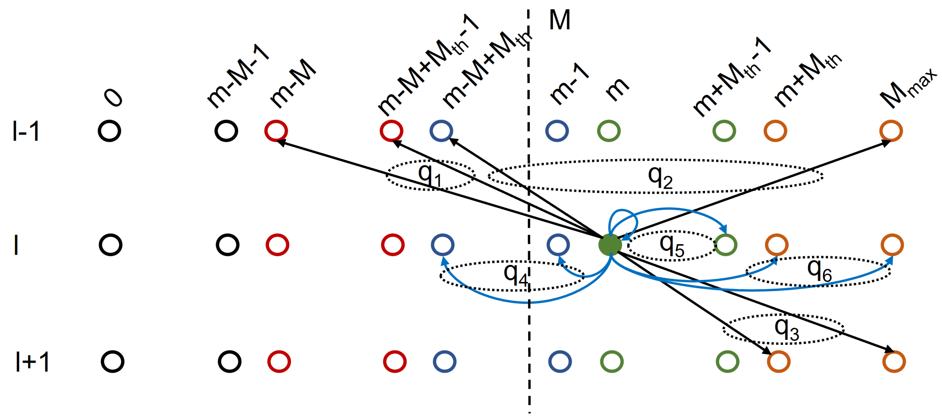
Figure 3.
OP performance for and . The solid and dashed lines correspond to the numerical and theoretical results, respectively.
Figure 3.
OP performance for and . The solid and dashed lines correspond to the numerical and theoretical results, respectively.
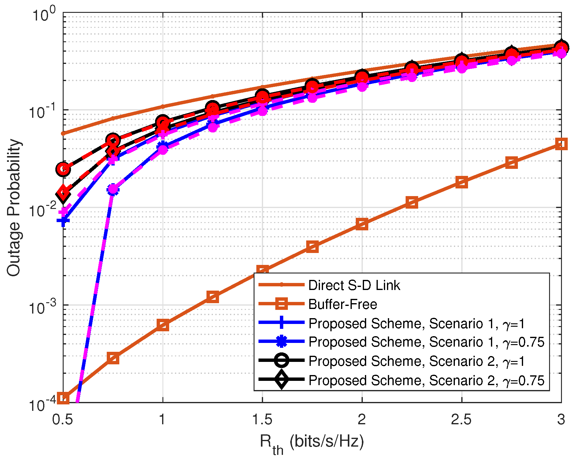
Figure 4.
Steady-State distribution of the number of packets stored in the data buffer for and bit/s/Hz.
Figure 4.
Steady-State distribution of the number of packets stored in the data buffer for and bit/s/Hz.
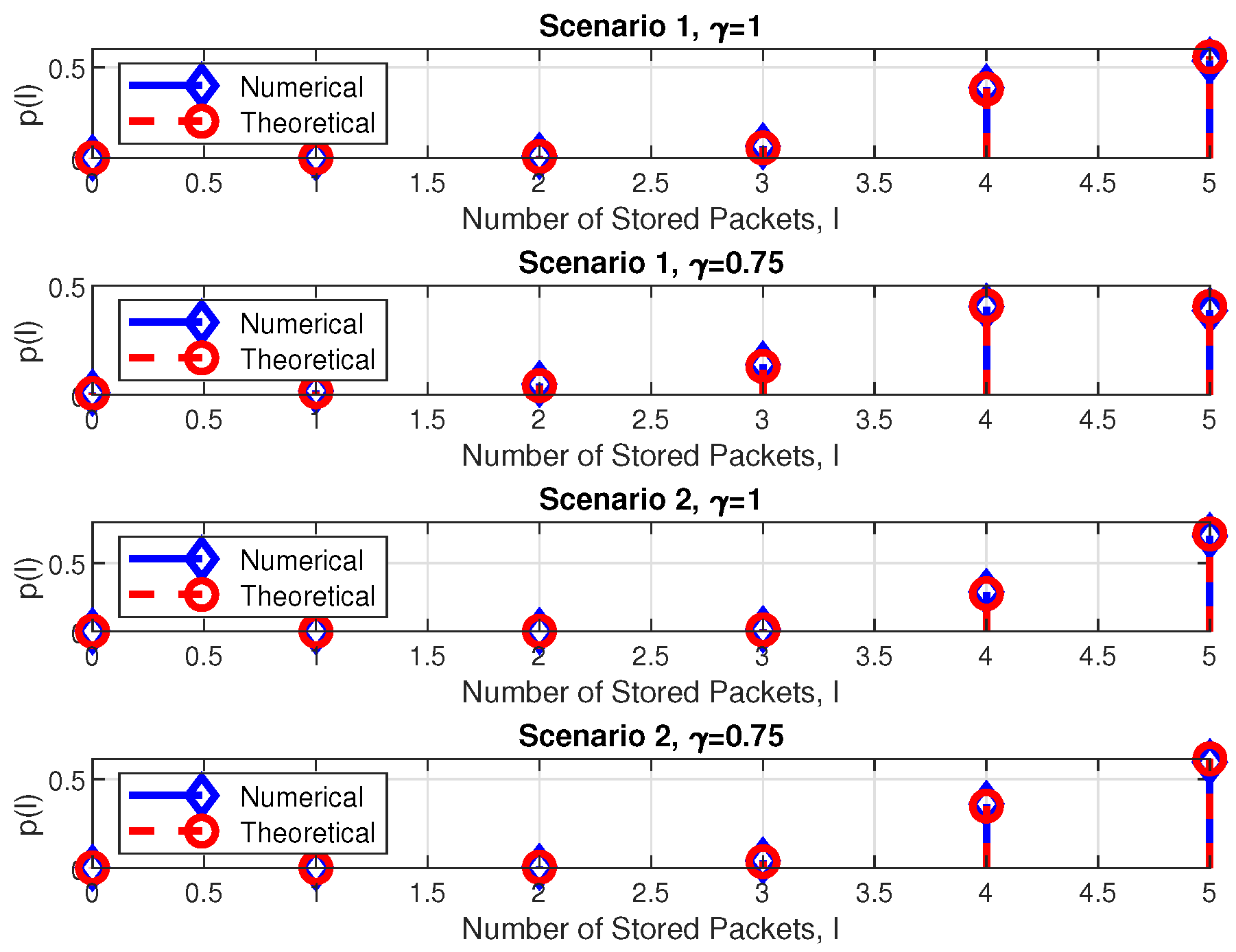
Figure 5.
Impact of the power factor on the OP performance for and bit/s/Hz.
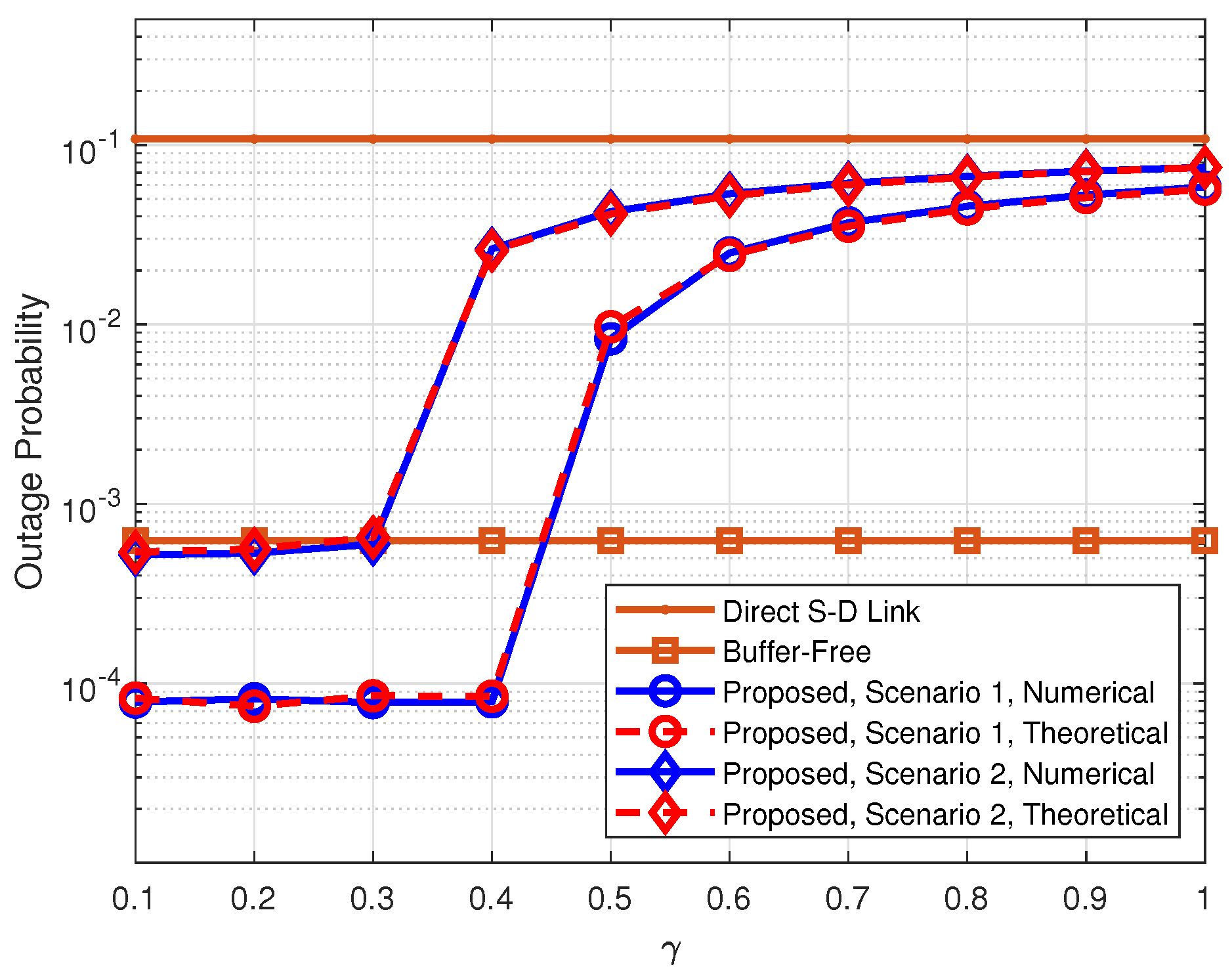
Figure 6.
Impact of the data buffer size L on the OP performance for bit/s/Hz.
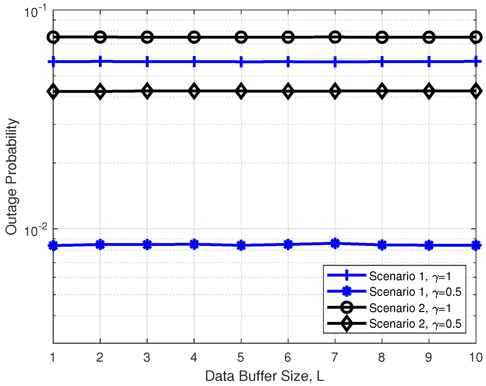
Figure 7.
Impact of the relay position on the OP performance for and a fixed S-D distance of 2.2 km.
Figure 7.
Impact of the relay position on the OP performance for and a fixed S-D distance of 2.2 km.
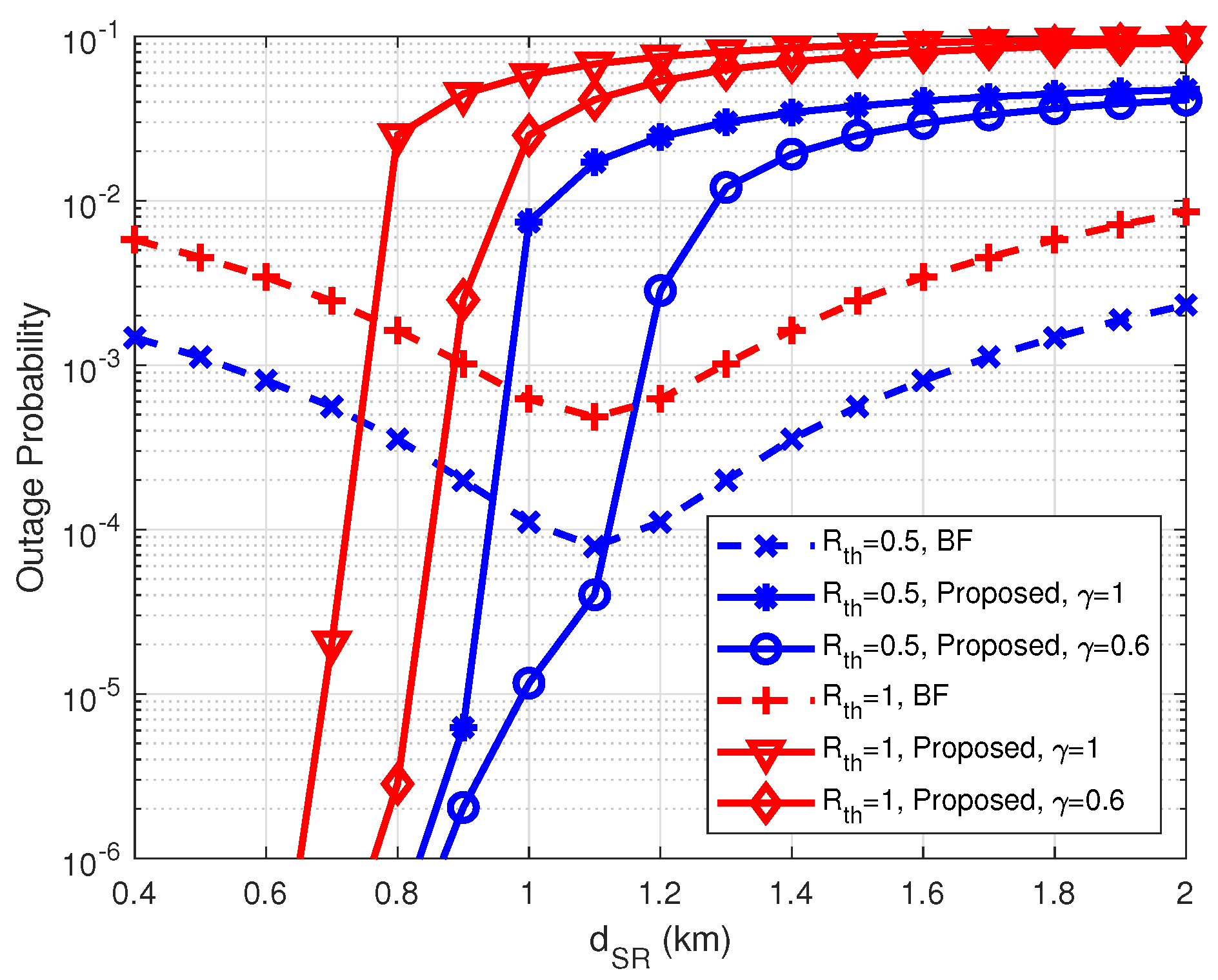

Table 1.
The simulation parameters
| Operating Wavelength () | 1550 nm |
|---|---|
| Receiver Responsivity () | 0.5 A/W |
| Peak Transmitted Power () | 50 mW |
| Noise standard deviation () | A |
| Receiving Area () | 0.05 m2 |
| Beam Angle () | 10 mrad |
| Attenuation coefficient () | 0.43 dB/km |
| RI structure parameter () | m−2/3 |
| Normalized pointing error | |
| displacement standard deviation () | 3 |
| Normalized beam waist () | 25 |
| Fill factor (f) | 0.75 |
| Dark saturation current () | A |
| Thermal voltage () | 25 mV |
Disclaimer/Publisher’s Note: The statements, opinions and data contained in all publications are solely those of the individual author(s) and contributor(s) and not of MDPI and/or the editor(s). MDPI and/or the editor(s) disclaim responsibility for any injury to people or property resulting from any ideas, methods, instructions or products referred to in the content. |
© 2024 by the authors. Licensee MDPI, Basel, Switzerland. This article is an open access article distributed under the terms and conditions of the Creative Commons Attribution (CC BY) license (http://creativecommons.org/licenses/by/4.0/).
Copyright: This open access article is published under a Creative Commons CC BY 4.0 license, which permit the free download, distribution, and reuse, provided that the author and preprint are cited in any reuse.


