Submitted:
03 December 2024
Posted:
03 December 2024
You are already at the latest version
Abstract
The minimalist approach in the study of perturbations in fluid dynamics and magnetohydrodynamics consists in describing their evolution in the linear regime using a single first-order ordinary differential equation, dubbed principal equation. The dispersion relation is found from the requirement the solution of the principal equation to be continuous and satisfy certain boundary conditions in each specific problem. The formalism is presented for flows in cartesian geometry and applied to classical cases, such as the magnetosonic and gravity waves, the Rayleigh-Taylor and Kelvin-Helmholtz instabilities. For the latter we discuss the influence of compressibility and the magnetic field, and also derive analytical expressions for the growth rates in the case of two fluids with the same characteristics.
Keywords:
instabilities
; fluid dynamics
; hydrodynamics
; magnetohydrodynamics
; methods: analytical
1. Introduction
The study of perturbations in any physical system sheds light into the mechanisms responsible for the equilibrium, and offers a way to predict its temporal behavior as a response to any variation. Being a difficult task in general, it is important to be able to simplify each case, focusing on the most important ingredients that determine its evolution. Classical waves and instabilities correspond to such simplified structures. For example acoustic compressible perturbations are attributed to sound or magnetosonic waves and can be identified even in systems with complex dynamics. Alfvén waves are important in magnetized plasmas. When gravity or buoyancy forces are important, differences in density drive gravity waves. And by “gravity” we could describe even fictitious forces in non-inertial frames, like the effective gravity in a decelerating system, or the centrifugal. In cases of heavy over light fluid stratifications immediately the Rayleigh-Taylor instability comes to mind. Similarly, a relative velocity between two fluids triggers the Kelvin-Helmholtz instability. These are only a few examples of simplified structures, that are nevertheless crucial in order to understand more complicated and realistic settings. They are often connected to temporal behaviors in laboratory experiments or particular features observed in astrophysical systems.
The full study of the perturbation evolution in most cases can only be done through numerical simulations. The linearization of the system of equations is a simpler way to understand under which conditions the system is unstable, although it does not cover the nonlinear evolution. Normal mode analysis is a further simplification, allowed only in symmetric unperturbed states, and can be used to find the wave frequencies or the instability growth rates. This allows a simpler parametric study, or even to have analytic expressions that directly show the physics of the mechanisms involved.
Since we are discussing classical problems, there are many books, e.g., [1,2,3,4,5], that provide the most basic information. There are also a plethora of related works in the literature over the years, e.g., [6,7,8,9,10,11] to name but a few. Nevertheless, these problems continue to be an active area of research, e.g., [12,13,14,15], and there is always room – and need – to improve our understanding.
The goal of this paper is to present the methodology to find the dispersion relation in each case, following the minimalist approach introduced in Ref. [16]. This novel approach simplifies the procedure as much as possible, since it uses a single first-order ordinary differential equation, dubbed principal equation. We first derive that equation through linearization and discuss the boundary conditions that need to be satisfied (Section 2). Then we apply the method to find the dispersion relation for MHD waves (Section 3), for gravity waves and the Rayleigh-Taylor instability (Section 4), for gravito-acoustic waves (Section 5), and for the Kelvin-Helmholtz instability (Section 6). We analyze the latter more extensively, deriving new analytical expressions for the growth rate in the magnetized case, and discussing the factors that affect most the results.
2. Linear Analysis, the Principal Equation, and Boundary Conditions
The non-relativistic ideal MHD equations in Lorentz-Heaviside units are
We are interested in exploring the perturbations of a steady-state that depends only on one spatial cartesian coordinate. In particular we assume that the unperturbed state has density , pressure , bulk velocity , magnetic field , and the acceleration of gravity is constant . Introducing the total pressure
the zeroth order equations are satisfied provided that
Adding perturbations of the form
defining the wavevector in the plane
and the Doppler-shifted frequency
we linearize the equations as shown in Appendix A; the main steps and related comments follow.
The linearized system reduces to two differential equations for the perturbations of the velocity in the direction and the total pressure (there are algebraic relations for all the other perturbations, connecting them to , , and their derivatives). Instead of and it is more convenient to use two other quantities.
The first, replacing , is the Lagrangian displacement in the direction. The relation between the Lagrangian displacement and the velocity perturbation results from the expression of the velocity in the perturbed location of each fluid element which equals , yielding . The component gives with .
The second quantity, replacing , is the perturbation of the total pressure in the perturbed location of each fluid element .
The advantage of these replacements is that the new functions and are everywhere continuous, even at locations where the unperturbed state has contact discontinuities.
2.1. The System for ,
The resulting system is
To simplify the expressions we define the following quantities that have important physical meaning and effect in the resulting dispersion relations through their appearance in the array elements .
The is connected to the angle between the wavevector and the unperturbed magnetic field. Its presence in a dispersion relation represents the influence of the magnetic tension which acts like a spring with restoring force per mass . This is evident in the pure Alfvén waves (in a static homogeneous plasma without gravity) for which the displacement satisfies with .
The appears in the denominator of the resulting system of differential equations, and its zeros correspond to the Alfvén waves.
The is related to the density perturbation in the perturbed location of each fluid element . It is interesting to note that the incompressible limit corresponds to .
The defined through represents the local wavenumber in the direction. Indeed, the latter equation is equivalent to the dispersion relation of the slow/fast magnetosonic waves if we define the total wavevector and the angle between and through .
Another way to see the connection between and the wavenumber in the direction is to consider the homogeneous fluid case without gravity, in which the system (14) (with constant coefficients in that case) has solutions . The equation gives two opposite solutions for corresponding to oppositely moving waves in the direction. Note also that in general is complex and its imaginary part corresponds to exponential variation of the eigenfunctions, since . In the incompressible limit in which and , it simplifies to purely exponential dependence (without sinusoidal dependence on x). More details on these waves will be discussed later; they offer a way to understand the physics of the solutions even in non-homogeneous fluids, and are directly related to the boundary conditions when the fluid extends up to large distances or .
The cases , , , need to be studied separately, something that can be easily done since they lead to simplified equations. They correspond to waves, and there is no need to be considered in instability studies in which is real and complex.
2.2. The Principal Equation
Since the system (14) is linear only the ratio is uniquely defined. Using the equations of the system we directly find that Y satisfies the principal equation
Following the minimalist approach it is sufficient to work with the ratio Y and solve the principal equation in order to find the dispersion relation of the wave or instability. We just need to integrate this single, first order differential equation, requiring Y to be everywhere continuous and satisfying the correct boundary conditions at the extreme values of x.
Knowing Y we can find all the other perturbations from
and the relations (A28)–(A35) given in Appendix A. We emphasize though that these are not needed to find the dispersion relation.
2.3. Boundary Conditions
The linearization was based on the functions and that are everywhere continuous. The same holds for their ratio, so in case of discontinuities of the unperturbed state we simply continue the integration of the principal equation when passing from one medium to the other keeping Y continuous.
In case where the fluid ends at some extreme value of x we always know the value of Y on that end and need to use it as a boundary condition. A first example of this kind is the case of a solid wall at that end, in which case Y vanishes on the wall since the Lagrangian displacement vanishes. A second example is the case when outside the fluid under consideration there exist a medium with constant total pressure, as for example in a hydrodynamic atmosphere with negligible density. In that case vanishes at the interface since the perturbation of the total pressure vanishes. (We arrive at the same result if we consider nonzero perturbation in the atmosphere, solve the problem in both sides requiring continuity of Y, and at the end take the limit of zero density outside.)
The nontrivial boundary conditions that need closer examination correspond to cases where the fluid extends to theoretically infinite distances or . At these distances the unperturbed fluid is homogeneous and the solutions of the principal equation are given in Appendix B. They correspond to two oppositely moving waves in the direction whose amplitude has an exponential dependence on x, one increasing and the other decreasing. In order to avoid the wave with the diverging amplitude1 the solution of the principal equation should also approach one of the constant values that correspond to complex wavenumbers , respectively. Assuming that is the principal value of the root (with positive real part) we choose the upper sign at and the lower at .
In case that (the is negative real number) the amplitude of the wave remains constant at infinity, and we can choose the solution whose sign of corresponds to the desired propagation.
The equations needed to apply the minimalist approach are summarized in Table 1.
Note that . In the presence of gravity this is not constant sine the unperturbed total pressure is variable with its gradient balancing gravity. However, in cases where the fluid extends to theoretically infinite distances (in which the total pressure also reaches theoretically infinite values) it approaches a constant corresponding to the incompressible limit.
In the absence of gravity and without loss of generality we can choose the sign such that (taking the principal value of the root and the upper/lower sign at , respectively).
3. MHD Waves
3.1. Slow/Fast Magnetosonic Waves
For homogeneous unperturbed state and zero gravity , , , and the principal equation becomes .
Its constant solutions are (both signs are allowed). According to equation (18) , i.e., is the wavenumber. The solutions corresponds to the continuous spectrum of the slow/fast magnetosonic waves, and as already stated, the equation is equivalent to the dispersion relation of these waves .
The variable solution of the principal equation corresponds to a superposition of waves as discussed in Appendix B.
3.2. Alfvèn Waves
The continuous spectrum of Alfvèn waves corresponds to the singular case of the principal equation . In that case could be any function of x, (and ), with finite and . (Note that for the Alfvén waves is given by , and does not represent a wavenumber.)
3.3. Two Semi-Infinite Incompressible Plasmas
As another example on how to use the minimalist approach lets consider two semi-infinite incompressible, homogeneous, static, magnetized plasmas in the regimes (subscript "1") and (subscript "2"), and zero gravity.
With in both regimes we have , , . The principal equation is and has constant solutions . According to the boundary conditions given in Table 1 (or directly checking the sign of ) the upper sign should be used for and the lower for . Thus for and for .
The continuity of Y gives the dispersion relation representing a stable Alfvén wave whose amplitude drops exponentially as we move away from the contact discontinuity at . (We remind that , , and that all the unperturbed states considered in the paper have the form described in Section 2.)
3.4. Effect of Finite Depth
Following the previous example, suppose now that the bottom plasma has finite depth H (there is a solid wall at ). Then in the bottom part the solution of the principal equation that vanishes at is . (In the upper part the accepted solution corresponding to vanishing amplitude at continues to be as before.)
The continuity of Y at gives the dispersion relation .
4. Gravity Waves and Rayleigh-Taylor Instability
Consider two semi-infinite incompressible, static, magnetized plasmas, the first (subscript "1") in the region and the second (subscript "2") in the region , inside uniform gravity , as in the left panel of Figure 1.
With in both regimes we have , , . The principal equation is and has constant solutions . (Although these parts are not homogeneous, since there must be a gradient of the total pressure balancing gravity, the incompressibility assumption allows to have constant solutions, provided that and A are constant in both parts.)
Choosing the correct sign in each part following Table 1 (or directly using ) we conclude that for and for .
The continuity of Y gives the dispersion relation .
This relation includes as subcases the surface gravity waves corresponding to zero magnetic fields and , for which , and the classical Rayleigh-Taylor instability corresponding to zero magnetic fields and heavier fluid on top of lighter, for which the growth rate is . It also shows the stabilizing effect of the magnetic field through its magnetic tension manifest in the dispersion relation in the presence of and . It always reduces the growth rate, and if it is sufficiently strong it makes positive, converting the disturbance from an instability to an Alfvén wave.
Effect of Finite Depth
If the bottom plasma has finite depth H (there is a solid wall at , see the right panel of Figure 1) we need to consider the variable solution of the principal equation with (given in Appendix B). Requiring Y to vanish at we find for .
As a specific example suppose the upper part is a hydrodynamic medium with negligible density. In that case for and the continuity of Y gives the dispersion relation for gravity waves , modified by the presence of the magnetic field. (The same can be found considering the constant solution in the upper part, requiring the continuity of Y at , and then taking the limit .) In the shallow water approximation we get .
5. Gravito-Acoustic Waves
In the examples presented up to now the fluids where homogeneous at least partially, allowing to easily solve the principal equation. In inhomogeneous cases we rely on the numerical integration of the principal equation. An exception to that, where it is possible to solve analytically the differential equation although the fluid is not homogeneous, is the case of gravito-acoustic waves. In addition it serves as a nice example showing the interplay between acoustic and gravity waves.
For a hydrodynamic fluid between two solid walls at and , inside homogeneous gravity , with unperturbed density , pressure satisfying the hydrostatic equilibrium condition , and the constant scaleheight, we get , , , and the principal equation can be written as
Its general solution is with , and the square of the Brunt-Väisälä (or buoyancy) frequency. The boundary condition specifies C and gives . The boundary condition requires , and the dispersion relation is .
The equation for is with solution .
(The cases and need to be examined separately. The former gives and the latter gives . Neither can satisfy the boundary conditions, so they cannot be accepted).
6. Kelvin-Helmholtz Instability
6.1. Incompressible Limit
For the incompressible case and two semi-infinite plasmas, similarly to the Rayleigh-Taylor instability (Section 4) we find that for and for . The only difference is that and now depend on the velocities.
The continuity of Y gives the dispersion relation with solutions
The three terms within the square root have obvious physical meaning. The first is due to relative velocity and always leads to instability. The second is due to gravity and leads to stability/instability in the case of stable/unstable stratification (lighter fluid above heavier or the opposite). The third term is due to the magnetic field stress and is always stabilizing.
6.2. Compressible Kelvin-Helmholtz Instability
Taking into account compressibility and neglecting gravity we have , , and the constant solutions of the principal equation are with . According to Table 1 we need to choose the upper sign in the and the lower in the . Thus and for , and for . The dispersion relation is , or,
(We remind that we need to take the principal values of both square roots, i.e., the ones with positive real parts.)
6.3. On the Physics of the Kelvin-Helmholtz Instability
A relatively simple case for which we can find analytical results will help to understand the physics of the instability. We consider two hydrodynamic fluids with the same unperturbed characteristics (same densities , same pressure as required from the equilibrium at the contact discontinuity, and same sound speeds ) and work in the frame where the two fluids move with opposite velocities (with positive and the upper sign corresponding to ).
The dispersion relation becomes , where . Unstable modes (with ) exist for , with purely imaginary . One way to find this result is to substitute when the dispersion relation reduces to with solutions . Actually the angle has an important meaning connected to the argument of the resulting complex wavenumbers in the direction, which are .
Although the results apply for any angle between and , to simplify the expressions from now on we restrict ourselves to the case , i.e., we consider a disturbance with (with positive ). The characteristics of the unstable mode, the Lagrangian displacement, and the perturbations of the pressure, density, and velocity (written in a way to show the phase difference between each quantity with ) are
Suppose we initially disturb the interface between the two fluids by . The Lagrangian displacement along at any later time and for any other fluid element has the form ; the goal is to find and . Using the Lagrangian displacement and the Lagrangian perturbations of the velocity, pressure, density, which are , , , respectively, the equations that will lead to that goal are the momentum and the continuity (coming from ). Since all perturbations are proportional to a time derivative has the meaning , and the divergence with the total wavenumber in the two fluids (their components are the same, but the components differ).
The momentum equation along connects the displacement with the pressure perturbation . Requiring and to be continuous at the interface between the two fluids we arrive at a first relation between the unknowns .
The pressure gradient along the interface is connected to the corresponding Lagrangian displacement through the momentum equation along , which gives . (The latter means that , a characteristic of longitudinal waves.)
The continuity also connects the two components of the displacement. It gives . Substituting and we arrive at the second relation between the unknowns (one for each fluid) .
The perturbation essentially consists of two sound waves in the two fluids with wavenumbers . In the fluid rest frames the two waves move with different velocities satisfying , a relation equivalent to with . The two waves meet at the contact discontinuity and as a consequence they have the same and such that their phases are continuous at the interface. As already presented, for the case of fluids with the same density, in a frame in which they move with opposite velocities , and is parallel to the relative velocity, the resulting unstable mode has and , with , .
The value of the complex wavenumber (in each part) is directly connected to compressibility through S. In the incompressible limit it is purely imaginary, since in that limit , and . (Note that in the incompressible limit the continuity gives . Since the two vectors are complex, this does not mean . It rather means , using from the momentum equation. In addition, the relation does not mean that the vector is zero.) If we consider cases with decreasing S, i.e., decreasing keeping the same, in which the compressibility becomes more and more important, the first part of the expression of affects the value of in two ways. Firstly the imaginary part decreases, meaning that the perturbation survives at longer distances from the interface. Secondly the increases contributing more to the phase of the perturbation which is . Both effects are expressed through the angle , which decreases with decreasing S (increasing M). The growth rate is also connected to S through . It decreases as the result of compressibility, from in the limit to zero when , corresponding to the minimum S for which the perturbation is unstable.
The vorticity is a key quantity in the Kelvin-Helmholtz instability. Its undisturbed value is the reason behind the development of the instability. Even with the perturbation included it is nonzero only in the interface between the two fluids. Nevertheless, the motion of the fluids along the interface redistributes the vorticity compared to the unperturbed state. The related velocity inside the upper/lower fluid, just above/below the interface , is . The mean value shows that fluid accumulates near the positions of lower pressure, where the vorticity increases (in the direction) by . This accumulation of vorticity further increases the displacement leading to instability. It becomes stronger for larger , i.e., smaller M, since the mean value of increases with .
Three example solutions are shown in Figure 2. The upper panel corresponds to an incompressible case with for which and . (For the approximate expression for is .) The exponential decrease of the perturbation as we move away from the interface is evident. The perturbed interface is shown, as also the circulation around points of minimum pressure (the mean velocity of the fluids on the interface points toward these minimum pressure points).
The two other panels correspond to cases in which compressibility is important. The solution in the middle panel has , and and in the lower panel , and . The has now a nonnegligible part and as a result the iso-phase planes are constant, tilted as shown in the panels.
For cases approaching the maximum value of M for which the perturbation is unstable (the ) the values of , and approach zero, and the perturbation practically consists of two standing sound waves (one in each fluid) with real wavenumbers. (For the approximate expression for is .)
6.4. Influence of Magnetic Field
For simplicity we consider again two homogeneous fluids with the same unperturbed characteristics, and work in the frame where the fluids move with opposite velocities . Now there is also a constant magnetic field in the unperturbed state, the same in both fluids.
Inspecting the dispersion relation (20) we see that the magnetic field enters in two ways. Firstly through its pressure , or equivalently the square of the Alfvén velocity . Secondly through its tension manifest in the terms , i.e. its component parallel to , or equivalently the component of the Alfvén velocity .
The magnetic pressure enters in the expression of S and increases its value. Thus it moves the dynamics toward the incompressible limit, and according to the discussion of the previous section destabilizes (the second terms inside the square roots equal , so increase of leads to the square roots being closer to unity). Actually if we include magnetic filed normal to only, the dispersion relation is exactly equivalent to its hydrodynamic analogue, with the only difference that M represents now the fast magnetosonic Mach number . Figure 3 shows the resulting growth rates. Notably it includes as subcases the purely hydrodynamic case () considered in the previous section, and the cold case () with only component of the magnetic field.
The magnetic tension enters in the dispersion relation through (essentially the component of the magnetic field along ) in two places: inside A and S. It always has a stabilizing effect since the tension is a restoring force; we have seen that in the previous examples of Alfvén waves and the Rayleigh-Taylor instability, even in the incompressible limit. It also affects incompressibility through its appearance inside S. Since it decreases S it moves the dynamics away from the incompressible limit, something that also in general stabilizes.
Another related connection is that the magnetic tension affects the perturbation of the vorticity inside each fluid, which, using the expressions of the velocity perturbations given in Appendix A, can be expressed as .
In the following we present the methodology to find numerical results.
The dispersion relation (20) in the case under consideration can be written as
and can be solved numerically. However, for the case of fluids with the same characteristics considered here it is possible to proceed analytically. As shown in Appendix C the dispersion relation can be transformed to the following quartic polynomial equation for the square of the growth rate
using the parametrization
(Note that the angle is connected to the angle between the magnetic field and the wavenumber since .)
The left panel of Figure 4 shows the growth rate for cases where the magnetic field has only component along . In general the field decreases the growth rate and if it is sufficiently strong completely suppresses the instability.
Similar behavior is shown in the right panel of Figure 4 for the cold case. For all strengths of the magnetic field, if its orientation is sufficiently close to the wavevector the magnetic tension completely suppresses the instability.
6.5. Range of Instability
It is interesting to explore the regions of M for which the Kelvin-Helmholtz instability is present, shown in Figure 4. The question is for which cases the dispersion relation (25) has purely imaginary roots. For simplicity we consider disturbance with parallel to the velocities, the results can be easily generalized.
One could naively think that the extreme values of these instability regions can be found by putting in the dispersion relation (25) and require both numerators to vanish (since the denominators are opposite real numbers). However this means and there is no x-dependence of the disturbance. That case corresponds to magnetosonic waves in the frame of each fluid with total wavevectors and with (see Section 3.1). The absence of x dependence makes these cases unrelated to the unstable modes.
However, there are two other possibilities. The vanishing of both denominators of the dispersion relation (25), for , needs to be considered as a possible limiting case. It corresponds to Alfvén waves with with (see Section 3.2). Note that does not enter in the dispersion relation. Nevertheless its value is nonzero . The x dependence of the disturbance allows for a possible connection with unstable modes.
A third possibility is to realize that the limiting values may correspond to bifurcations of the dispersion relation. It is actually evident from inspection of Figure 3 that the slope becomes infinity when . A dispersion relation in general depends on various parameters, and the slope is meant as a derivative with respect to one of them keeping constant all the others. For a dispersion relation of the form constant its differential shows that bifurcation corresponds to . Thus, extreme values of the instability regions may be connected to the condition .
In our case there are three parameters, and we can choose , , . The algebra gives that leads to , or the following cubic for
or, .
For the left panel of Figure 4 we have , , and the extreme values of M are given by . The roots are , , , and the corresponding wavenumbers , , , respectively. Thus the value corresponds to a magnetosonic wave without x dependence (unrelated to instability), while the other two solutions , are the extreme values of M related to the unstable modes.
The result is that for the Kelvin-Helmholtz instability occurs only if and for velocities in the interval . As we approach the limits the wavenumbers approach real values and the instability is transformed to magnetosonic waves with constant amplitudes and wavenumbers .
For the right panel of Figure 4 we have and and the maximum value of M corresponds to bifurcation for which . The nontrivial root is , and the corresponding wavenumbers .
The lower limit of the instability region corresponds to Alfvén waves so .
The result is that for the cold case the Kelvin-Helmholtz instability occurs only if . As we approach the limits the wavenumbers approach real values and the instability is transformed to waves (Alfvén wave in the lower limit and magnetosonic in the upper) with constant amplitudes and wavenumbers .
6.6. Bifurcations in the General Case
The dispersion relation in the general case is , and taking its logarithmic derivative we conclude that bifurcations occur when is continuous at the interface. Equivalently, since is also continuous, is continuous. Substituting S and this quantity equals
.
In the hydrodynamic case the latter simplifies to , while in the cold case to .
7. Summary
The main goal of the paper is to present the minimalist approach in stability problems with planar geometry that can be described using cartesian coordinates. It shows the power of the approach in finding the dispersion relation by integrating a single first-order differential equation, the principal equation.
The mathematical formalism is quite cumbersome, but can be made easier by defining intermediate quantities with important physical meaning. For example the complex has a direct connection to wave propagation and simultaneous amplitude variation. The function S is connected to the compressibility that depends on both, the thermal and magnetic pressure, and shows how the wave propagation and the growth rate of the instability depend on them. The function F is the signature of the stabilizing nature of the magnetic tension. All these are discussed and reviewed when applying the method to the classical instabilities.
A more extensive analysis was done on the Kelvin-Helmholtz instability, for which new results were also found. Namely analytical solutions of the dispersion relation in certain cases, as well as the study of bifurcations and their connection to the ranges of instability. These tools make much easier the parametric study, which is far from being considered complete even in classical instabilities.
Detailed studies of specific problems in hydrodynamics or magnetohydrodynamics hopefully will benefit from the examples and the formalism presented, but also from the ideas how to explore possible existence of analytical solutions and specify the range of instability. Applications in other geometries and more general theoretical frameworks are also possible and will be presented in other connections.
Funding
This research received no external funding.
Data Availability Statement
This research is analytical; no new data were generated or analyzed. If needed, more details on the study and the numerical results will be shared on reasonable request to the author.
Conflicts of Interest
The author declares no conflicts of interest.
Appendix A. Linearization
The linearized Equations (1)–(4) are (for )
with , the sound speed (only the unperturbed is needed and is assumed known function of x), , In the above expressions the relation was used. This can be seen as a consequence of the induction Equation (4), but shows more directly that the relation holds.
Using the last three Equations (A6)–(A8) and substituting we can express the perturbations of the magnetic field as
Substituting these in Equations (4) and (5) we find
where . Substituting these in Equations (A10) and (A11) we find
and in Equation (A1) we find
Thus the system becomes
We introduce the perturbation of the total pressure in the perturbed position , a quantity that is continuous everywhere (similarly to ).
Equation (18) in combination with Equations (23) and (24) and the equilibrium of the unperturbed state can be replaced with
where . Equations (A17) and (A19) give the system for and
where , and we arrive at the equations (14).
After solving this system and find , we return to the rest of the equations and find all other perturbations. We summarize the expressions below (in which the left-hand sides represent the Lagrangian perturbation of each quantity, i.e., the perturbation in the perturbed position).
Appendix B. Solutions of the Principal Equation in the Homogeneous Case
If the array elements are constants the principal equation has two kind of solutions. Either constants satisfying with , or variable , with a constant of integration.
Each one of the former corresponds to one way wave propagation in the (or ) direction and the latter to a superposition of these two waves. This becomes clear if we find and using Equation (18). It is even simpler to look for solutions of the system (14), which is linear with constant coefficients in this case and admits solutions of the form with . The general solution is , .
We can simplify the expressions of the eigenfunctions to , , substituting , and their ratio agrees with the solution of the principal equation given above . Note that the last expression for Y can also be written as with , and we get the equivalent expressions of the eigenfunctions , .
The constant Y solutions correspond to , giving , .
The complex wavenumbers of the two waves are . Taking the principal value of the square root (with positive real part), the upper/lower sign corresponds to a wave whose amplitude decreases with increasing/decreasing x.
Appendix C. Analytical Solutions of the Magnetized Kelvin-Helmholtz Instability
With the parametrization , , , , , the dispersion relation (25) becomes
We can analytically find purely imaginary solutions of that equation, which is the continuity of the ratio . First we observe that if the fluid characteristics are the same in the two parts and the velocities opposite, for purely imaginary , i.e., real , the relations and hold. This means that the dispersion relation is equivalent to the requirement the ratio to be real.
We can write the numerator as , with such that the amplitude vanishes at . In order for the ratio to be real, should be real.
Substituting the expressions of and A, the previous two relations mean that the imaginary parts of and are zero.
Thus we arrive at the two relations that give in parametric form with parameter
Eliminating we find a single relation for the growth rate, the quartic polynomial Equation (26).
Note that the Equation (26) can also be derived by squaring Equation (A36), since the substitution helps to exclude the trivial solutions of the resulting polynomial. This proves that indeed the solution is purely imaginary and verifies the above derivation, which has the advantage of connecting the solution with the correct sign of and its argument .
| 1 | There is a way to automatically find the non-diverging solution following the Schwarzian approach of Ref. [17]. To get analytical expressions though, as we attempt here, we can directly find use the asymptotic solutions. |
References
- Chandrasekhar, S. Hydrodynamic and hydromagnetic stability; Oxford: Clarendon Press, 1961. [Google Scholar]
- Boyd, T.J.M.; Sanderson, J.J. Plasma Dynamics; Nelson, Great Britain, 1969.
- Bateman, G. MHD instabilities; 1978.
- Freidberg, J.P. Ideal MHD; 2014. [CrossRef]
- Goedbloed, H.; Keppens, R.; Poedts, S. Magnetohydrodynamics of Laboratory and Astrophysical Plasmas; Cambridge Univ. Press, Cambridge, 2019.
- Ferrari, A.; Trussoni, E.; Zaninetti, L. A&A1978, 64, 43.
- Hardee, P.E.; Norman, M.L. Spatial Stability of the Slab Jet. I. Linearized Stability Analysis. Astroph. J. 1988, 334, 70. [Google Scholar] [CrossRef]
- Osmanov, Z.; Mignone, A.; Massaglia, S.; Bodo, G.; Ferrari, A. On the linear theory of Kelvin-Helmholtz instabilities of relativistic magnetohydrodynamic planar flows. Astron. Astrophys. 2008, arXiv:astro-ph/0802.2607490, 493–500. [Google Scholar] [CrossRef]
- Matsumoto, J.; Aloy, M.A.; Perucho, M. Linear theory of the Rayleigh-Taylor instability at a discontinuous surface of a relativistic flow. Mon. Not. R. Astron. Soc. 2017, arXiv:astro-ph.HE/1707.04706472, 1421–1431. [Google Scholar] [CrossRef]
- Papadopoulos, D.B.; Contopoulos, I. The magnetic Rayleigh-Taylor instability around astrophysical black holes. Mon. Not. R. Astron. Soc. 2019, arXiv:gr-qc/1811.09086483, 2325–2336. [Google Scholar] [CrossRef]
- Gourgouliatos, K.N.; Komissarov, S.S. Relativistic centrifugal instability. Mon. Not. R. Astron. Soc. 2018, arXiv:astro-ph.HE/1710.01345475, L125–L129. [Google Scholar] [CrossRef]
- Chow, A.; Rowan, M.E.; Sironi, L.; Davelaar, J.; Bodo, G.; Narayan, R. Linear analysis of the Kelvin-Helmholtz instability in relativistic magnetized symmetric flows. Mon. Not. R. Astron. Soc. 2023, arXiv:astro-ph.HE/2305.00036524, 90–99. [Google Scholar] [CrossRef]
- Karampelas, K.; Van Doorsselaere, T.; Guo, M.; Duckenfield, T.; Pelouze, G. Kelvin-Helmholtz instability and heating in oscillating loops perturbed by power-law transverse wave drivers. Astron. Astrophys. 2024, arXiv:astro-ph.SR/2406.11700688, A80. [Google Scholar] [CrossRef]
- Nykyri, K. Giant Kelvin-Helmholtz (KH) Waves at the Boundary Layer of the Coronal Mass Ejections (CMEs) Responsible for the Largest Geomagnetic Storm in 20 Years. Geophysical Research Letters 2024, 51, e2024GL110477. [Google Scholar] [CrossRef]
- Jiang, Q.; Li, G.X.; Singh, C.B. Dispersion relation for the linear theory of relativistic Rayleigh Taylor instability in magnetized medium revisited. 2024; arXiv:astro-ph.HE/2411.03347. [Google Scholar]
- Vlahakis, N. Linear Stability Analysis of Relativistic Magnetized Jets: The Minimalist Approach. Universe 2024, arXiv:astro-ph.HE/2404.1061310, 183. [Google Scholar] [CrossRef]
- Vlahakis, N. The Schwarzian Approach in Sturm-Liouville Problems. Symmetry 2024, arXiv:math-ph/2405.1254916, 648. [Google Scholar] [CrossRef]
Figure 1.
The unperturbed state of two fluids in contact at . Left panel: semi-infinite fluids. Right panel: the bottom part has finite depth H.
Figure 1.
The unperturbed state of two fluids in contact at . Left panel: semi-infinite fluids. Right panel: the bottom part has finite depth H.
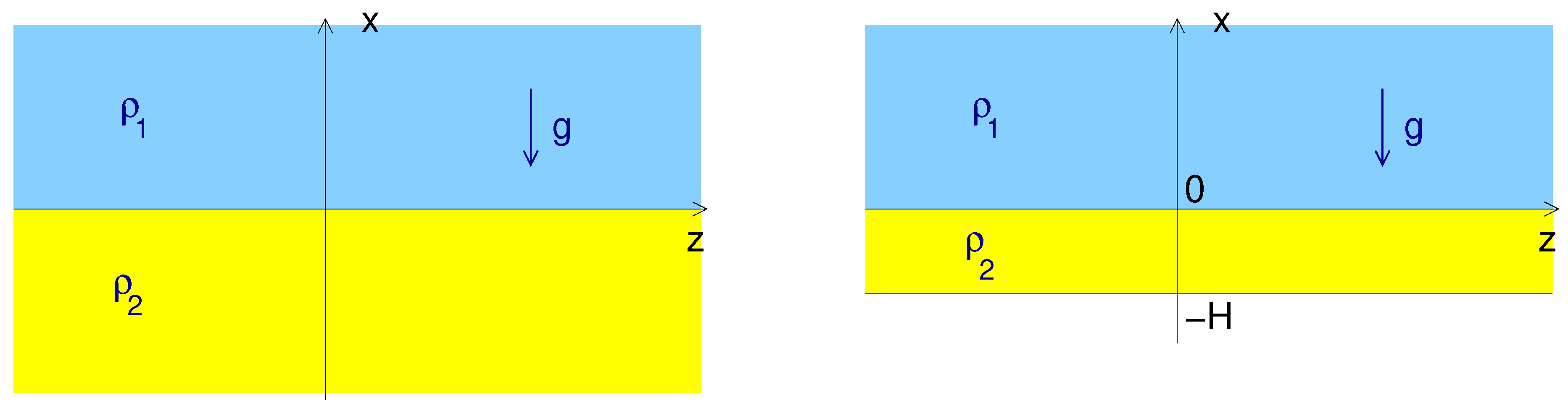
Figure 2.
The streamlines and the pressure perturbation for three cases, (upper panel), (middle panel), and (lower panel).
Figure 2.
The streamlines and the pressure perturbation for three cases, (upper panel), (middle panel), and (lower panel).
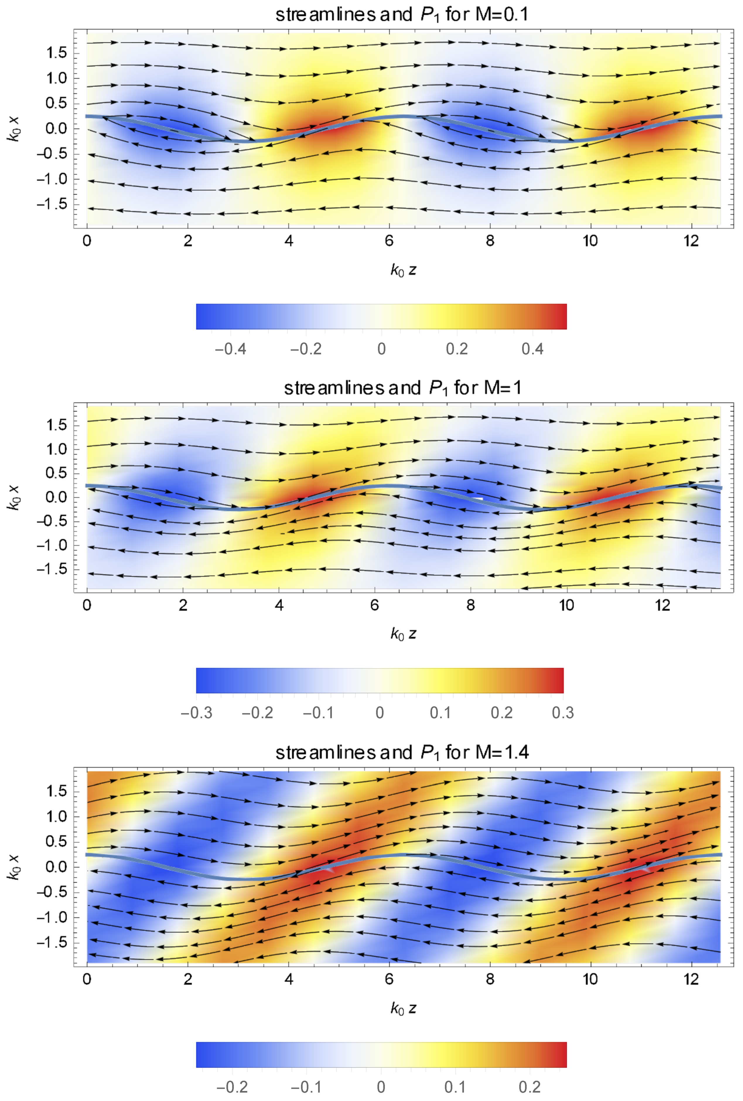
Figure 3.
The growth rate of the Kelvin-Helmholtz instability for two homogeneous fluids moving with , with same unperturbed density , sound speed , magnetic field , and disturbance with .
Figure 3.
The growth rate of the Kelvin-Helmholtz instability for two homogeneous fluids moving with , with same unperturbed density , sound speed , magnetic field , and disturbance with .
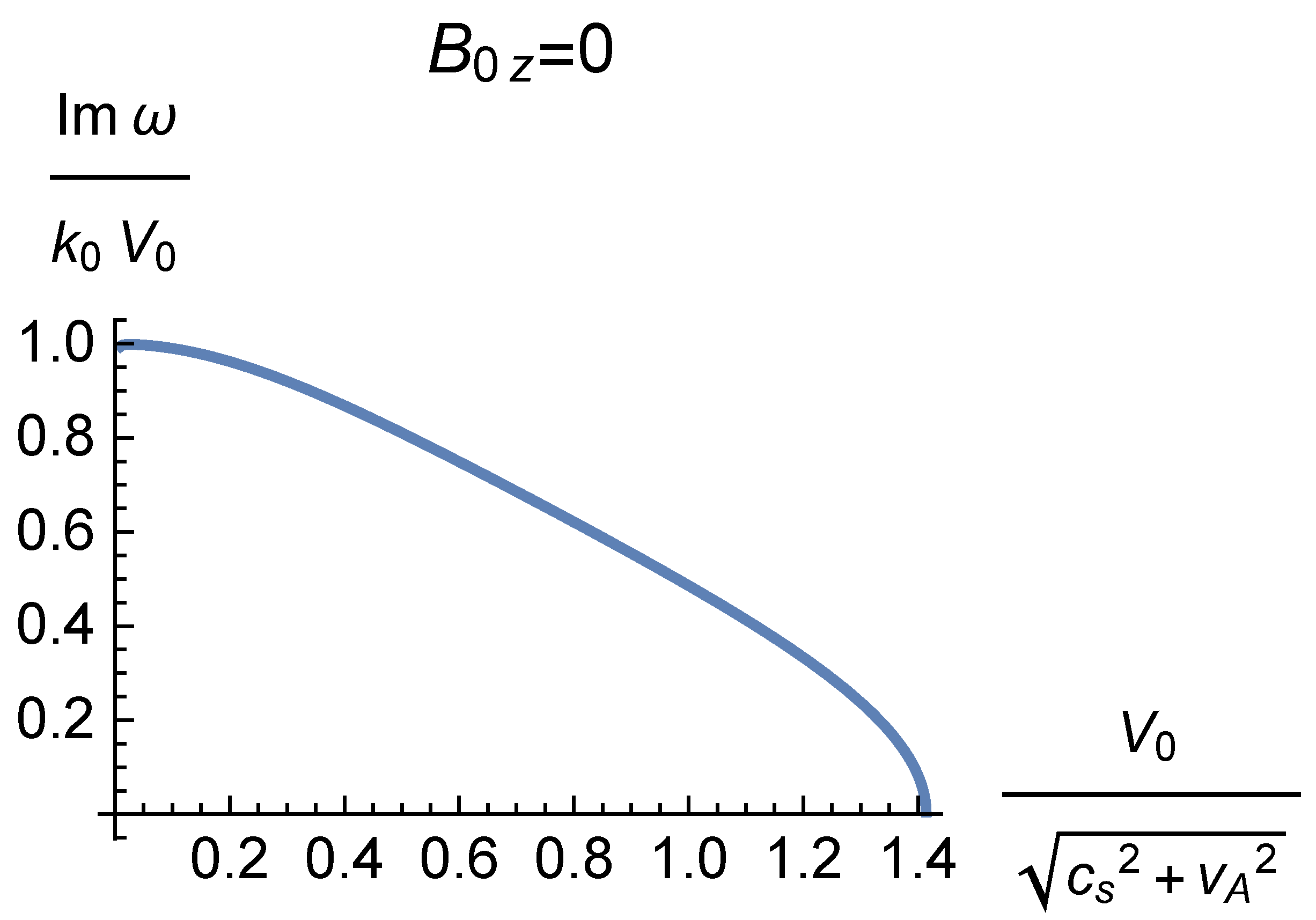
Figure 4.
Same as Figure 3, but in the left panel for magnetic field along with various strengths corresponding to the shown values of the ratio , and in the right panel for cold cases () and magnetic field with various strengths and orientations corresponding to the shown values of the ratio (in all cases ).
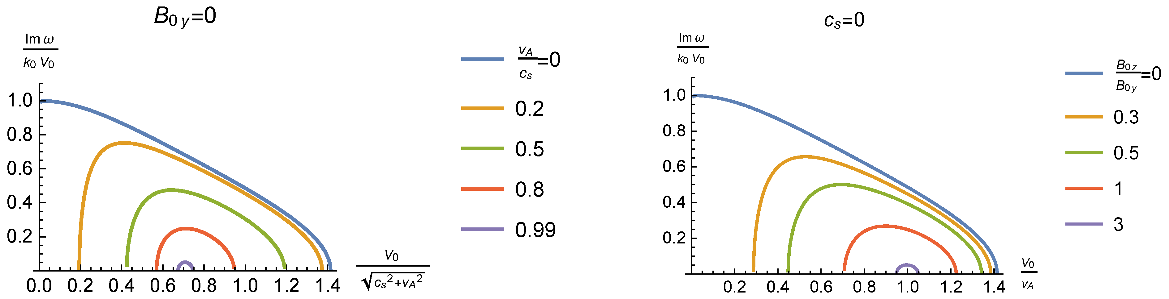

Table 1.
Minimalist approach equations and boundary conditions.
| Principal equation: | |
| with | |
| Boundary conditions: | Y continuous everywhere, asymptotically |
Disclaimer/Publisher’s Note: The statements, opinions and data contained in all publications are solely those of the individual author(s) and contributor(s) and not of MDPI and/or the editor(s). MDPI and/or the editor(s) disclaim responsibility for any injury to people or property resulting from any ideas, methods, instructions or products referred to in the content. |
© 2024 by the author. Licensee MDPI, Basel, Switzerland. This article is an open access article distributed under the terms and conditions of the Creative Commons Attribution (CC BY) license (https://creativecommons.org/licenses/by/4.0/).
Copyright: This open access article is published under a Creative Commons CC BY 4.0 license, which permit the free download, distribution, and reuse, provided that the author and preprint are cited in any reuse.


