
Submitted:
04 December 2024
Posted:
05 December 2024
You are already at the latest version
Abstract
Reinforcement learning is a major branch of machine learning which uses sequence of past experiences, to help a system learn and predict optimal behaviour. There are multitude of proposed learning procedures that have attempted to perform such learning. While typical prediction problems utilized the final outcome to minimize the error, Sutton explores ”temporally successive predictions” to assign credit for the actions performed. Similar to a weather forecast for the weekend getting better as time progresses, TD (Temporal Difference) learning utilizes the same method of updating estimates every time step to progress towards the optimal value. This technical report discusses the background and intuition behind the original paper [1] by recreating the experiments and investigates the reproduced empirical results to compare and contrast the assumptions and findings described in the original literature.
Keywords:
supervised learning
; reinforcement learning
; temporal difference
; reproducibility
; technical report
1. Introduction
Supervised learning was used to solve most problems including temporal (time step based) updates with data being the current time step with the label identified based on the actual outcome or simply the next time step. However, such methods lose the transference of the temporal nature of these data points leading to a very poor learning experience and generating poor results for testing data sets or future predictions.
This paper focuses on TD (Temporal Difference) based learning as a method for numerical predications unlike earlier discussions [2], which focused on Inductive learning to predict diagnostic rules, or predicting the next character from a partially generated sequence. Rather this paper demonstrates the ability to perform prediction based on numerical attributes in combination with weight parameters. Another aspect of this paper is the focus on multi-step temporal problems rather than single-step problems as their novelty is better demonstrated on multi-step problems.
1.1. TD (Temporal Difference)Algorithms
The classical Windrow-Hoff rule is used as the baseline for comparison to the TD and supervised learning algorithms. Both Widrow-Hoff and TD generates the same set of weight changes, however the first experiment shows how TD achieves this in an incremental fashion. The next experiments demonstrate how TD() produces a varying range of weight changes enabling the process to identify the best suited parameters with higher accuracy ranges than any supervised learning procedure.
A typical multi-step problem is constructed as a set of observation vectors and their outcome such as where represent the observations while z indicates the outcome. Since the TD is an incremental and temporal based algorithm, it equivalently produces a vector of predictions representing an estimate of z at that time instance. The predictions can be constituted as function of all the earlier predictions and outcomes along with the current sequence, though for this particular discussion, P is determinant only on the current sequence of observations captured as , represented as as this is also considered to be a Markovian process.
The algorithm uses function approximation by using modifiable weights w as part of the predictions, formulating predictions as a function of and w. The intuition lies in the repeated presentations of experiences/observations to learn the appropriate weights, to learn the variance with low bias, and predict outcomes based on future observations. This learning structure enables the algorithm to define the learning process as updates to the w weights vector.
The update process to the weights w, after each observation is determined by , representing an increment/decrement to the weights and at the end of each observations-outcome pair, the is applied to the weights as . The paper also demonstrates both incremental updates to the weights and delayed updates after accumulating over a training set of multiple sequences. A simple depicting of how TD algorithm learns the true values after multiple presentations, is depicted in Figure (Figure 1), where the number of presentations increase and the predictions get closer to the true value.
1.1.1. Comparison with Supervised Learning
Supervised learning treats the observation outcome sequence as pairs such as while the weight updates are determined based on the error between the predictions at each time step, and the rate of error updates is determined by a learning rate () and given as where represents the partial derivatives of with respect to each w. If the predictions are considered a linear function (similar to above) of w and at each time step t, then they can be represented as and performing a partial derivative of this equation with request to on both sides, converts the equation to and substituting these two values in the expression gives us the Widrow-Hoff rule , also known as the delta rule.
The intuition lies in the error difference between the actual outcome z and the prediction , represented by and its weightage by the observation vector to determine the direction and magnitude of the weight updates to minimize the error. This intuition directly translates to TD, where the error difference between current prediction and outcome can be computed incrementally as a sum of difference in predictions where each depends only on each successive prediction pairs and previous values of as (2)
1.1.2. Extension of TD to TD() Algorithms
While TD discussed until now, utilizes all the previous values of , the paper introduces a more wider range of tuning capability in the TD algorithm with the introduction of , representing the dynamic weightage applied to , representing the temporal difference predictions. The TD() algorithm garners more sensitivity to the most recent prediction change while a lower weightage to a prediction change few steps earlier, using an exponential weighting based on their recency and frequency heuristics. Introducing the new parameter and updating the earlier equation produces (2)
Having , represents equal weightage and generates the same equivalent equation to the Widrow-Hoff rule and defined as TD or TD(1).
While TD(1) utilizes all the previous predictions, TD(0) where , essentially utilizes only the most recent observation to determine the weight update and represented as . .This provides the intuition that any value for between will produce different weight changes and their error rates with the outcome would be different based on the problem space and available training datasets etc., These equations clearly demonstrate the ability of TD to benefit from the temporal structure of the observations which typical supervised learning algorithms ignore.
1.1.3. Instability Prevention for Incremental Updates
As illustrated above, TD learning method performs incremental weight updates every step, using the weighted previous predictions. However, as the paper explains, intra-sequence updates such as where is represented by (1) need to be handled carefully, since they are influenced by the change in the observation and the as well, which would lead to instability. To prevent the instability due to such oscillation of weight values, the equation is modified to update the weights only for predictions generated by , the observation involved. The modified equation is given by (3)
1.1.4. Note on Lambda () and Discount Factor ()
In a MRP (Markov Reward Process) or MDP (Markov Decision Process) the discount factor () helps determine the value function for a particular state based on immediacy of the rewards. It helps compute the value applicable to a particular state dependent on its distance from the actual reward available in the future, immediate or delayed i.e., , the discount factor, helps weigh delayed rewards versus immediate rewards and determine value functions for a state. The parameter helps in evaluating the right level of bias to be adopted in choosing the previous predictions to be utilized, while predicting the outcome based on recent observation. Intuitively, the discount factor () helps determine the objective to be achieved in the MDP, by discounting possible future rewards to help determine a particular action in MDPs or compute the value function for a MRP. The discount factor is independent of parameters of a learning algorithm and specifically used as part of the MDP definition itself. The lambda () parameter on the other hand functions similar to a hyperparameter of a learning algorithm, lower the errors to the least minimum possible. However, they function outside the MDP and influence only the range of the learning algorithm and does not affect the reward function.
1.1.5. Temporal Difference (TD) Comparison with Widrow-Hoff & Monte Carlo
Similar to TD, Monte Carlo represents a set of methods to solve learning problems based on averaging sample returns and utilized in reinforcement learning similar to TD learning. The primary contrast between TD and MC methods, are the incremental prediction updates performed in TD, while MC methods requires the experience of a completed episode with actual returns as part of their learning procedure. While TD perform updates during the sequence of the observations, MC would update only at the completion of an episode and hence cannot be used in an online learning system. Widrow-Hoff and TD learning are similar in the aspect of being online-learning procedures since the perform updates based on the observations and primarily move towards minimizing the RMSE for the observation-outcome pairs. However, whereas Widrow-Hoff is modelled as a linear function, Monte Carlo methods are more generalized for any model-free learning problems. Though TD(1) and Widrow-Hoff produces the same updates, as per the paper, TD can be generalized as well to perform learning for non-linear functions. As Sutton & Barto note in [3], TD learning is biased towards the parameters and the bootstrapping performed, and runs the risk of high bias. While Monte Carlo does not have this issue, it suffers from high variance and requires a large number of samples to achieve similar levels of TD learning. In conclusion, though Monte-Carlo performs very similarly to TD(1), there are subtle differences in their learning process and underlying assumptions.
2. Random Walk Problem
A Markov chain in [4] is described as a sequence of possible stochastic events in which the probability of each event depends only on the state attained in the previous event. In continuous-time, it is known as a Markov process. Markov Reward Process (MRP) extends the Markov chain by adding a reward rate to each possible state. The paper utilizes one of the simplest dynamic model systems, which generates bounded random walks, to demonstrate that the TD methods are more efficient and learns faster than supervised learning. The bounded random walk MRP demonstrates the Markovian property where each state depends only on its previous state. The random walk depicts a set of terminal states and non-terminal states with transition probabilities that can be observed over time which can be utilized to predict their values using TD.
A bounded random walk with 7 states, depicted in Figure (Figure 2), always begins in the middle state D and determines the action of going left or right to its neighbour based on a random policy with equal probability until it reaches one of the terminal states A or G. If the walk reaches the terminal state G, then the MRP terminates and receives a reward of 1 , while on reaching terminal state A, the outcome is determined as 0 .
The learning problem is structured around this reward outcome where the expected value functions of each state would be equal to the probability of reaching state G from each of these states i.e., the probability of reaching G from B,C,D,E and F would be and respectively. For simpler computation purposes, each state within a sequence of random walk was represented as a unit basic vector of length 5 with the position representing the current state. For example, the state B was represented as while state E was noted as . When the walk is at a particular state where its "1" is at the component of the observation vector, the prediction at time t, is simply the value of the component of the weight vector w since as depicted in Figure (Figure 3). This one-hot encoding structure helps with applying the incremental updates only for predictions generated by . The MRP is undiscounted for their future rewards and has a discount factor () as 1.
3. Experiments
The paper performs three computational experiments to analyze the capabilities and performance of TD() algorithm on the bounded random walk MRP in comparison with supervised learning Widrow-Hoff rule. The experiments also expand on the role of the parameter and how each specific MRP can have optimized specific values. To provide reliable results, the paper generates training data with 100 training sets, where each training set consists of 10 sequences and every sequence represents a terminated episode of bounded random walk as illustrated in Figure (Figure 4). Though, the original paper does not mention the parameters used for training dataset generation, the algorithms are generalized sufficiently to converge on appropriate values as demonstrated in the later section of this paper. Though not specified in the original paper, sequences are limited to a length of 20 to derive similarity with the original paper results. Limiting the sequence length, helps ensure that TD(0) or lower values get reward propagation quick enough to reproduce the results. These experiments are implemented as "Forward view", where the updates for next states are performed incrementally. However, as the original paper states, performing these experiments using "backward view" should not alter the results.
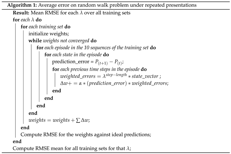
3.1. Experiment 1 – Convergence with Repeated Presentations
The first experiment performs "repeated presentations" of the training data, using the TD() learning procedure, and gathers the average error against a range of values from (the Widrow-Hoff procedure) and (one-step linear TD) and intermediate values between 0 and 1. Performing weight updates within a walk sequence, poses the risk of probable instability with continuous weight alterations, without any convergence. In order to prevent the instability and ensure convergence of weights for each value, as the original paper suggested, the algorithm accumulated the weight differences over a complete presentation of a training set and then the weights are updated for the next training set, rather than being changed within the execution of a sequence itself. Each training set was repeated until there were no changes to the weight vectors within tolerance and termed as "repeated presentations" as depicted in Figure (Figure 5)
3.1.1. Description and Implementation
As suggested in the paper, a very low value of learning rate () of 0.0044 was used to ensure that the weight vectors converged to values closer to the originally presented results. To measure the performance of the learning procedure, the root mean squared (RMS) error was computed comparing the ideal values for each state and the predicted values by TD learning process for various values of . The step-by-step procedure is available in Algorithm (1), while Figure (Figure 5) depicts the application of weight updates after the complete presentation of a training set each with 10 sequences after convergence of weight changes. The convergence of weights is determined by measuring the maximum difference of weight update between iterations to be lesser than a threshold of 0.001.
3.1.2. Results
The original results from the paper (deduced from the image) and the reproduction results are plotted together for comparison in Figure (Figure 6). On plotting the results, a surprising discovery is the poor performance of TD(1) which generates the same weight updates as Widrow-Hoff. Since TD(1) has the actual outcome available before making the predictions, conventionally, they should have exhibited the least RMSE. However, on introspection, as the paper denotes, the TD(1) is biased by the observation-outcome pairs provided as training dataset and minimizes error only for the provided data, similar to the overfitting phenomenon observed in supervised learning. However, TD(0) on the other hand converges to the optimal estimates with significantly lesser error than TD(1), in line with the maximum likelihood estimate of the Markov Reward Process.
3.1.3. Observations and Analysis
The results were in line with the original results made available in the paper. The values for TD(0) converged to the likelihood estimates around 0.19 similar to the paper. However, for higher values of , especially for 0.9 and 1.0, the error values were slightly higher (for TD(1), 0.28 instead of 0.25). This can be attributed to the randomness of the training data set used and also the sequence run lengths being generated in the training data sets. TD(1) as described attempts to overfit the training dataset initially and for longer sequences, incurred more bias leading to a higher RMSE values. However, for lower values (), the reproduction results were close to the original paper with deviations less than 0.01 as illustrated in Figure (Figure 6).
3.1.4. Parameter Determination – Learning Rate
One of the key parameters, learning rate (), was not made available as part of the original paper and plays an important role in the determination of the RMSE. This value determines the rate at which the weight adjustments are assimilated by the learning procedure. To ascertain, the best value for the random walk example, since the 100 training set consists of 10 sequences each, an experiment inspired by the random walk example in [3] was conducted to identify the RMS Error over 1000 episodes for different values of and also evaluate the convergence of TD(0) algorithm over these episodes. As illustrated in Figure (Figure 7), 0.001 was way too slow to converge within 1000 episodes, while higher values overfit the training data quickly producing higher errors. The value of performed well with high error at the beginning and converging to low RMSE error at the end of the training episodes.
3.1.5. Standard Error
The paper notes the standard error of results as 0.01, which helps in verifying the statistical validity of the results being within a 0.01 range of variance and estimates the variability between samples of the RMSE values for each . All the calculated values in this experiment have a standard error less than 0.01 while only had a slightly higher value of 0.011 as illustrated in Figure (Figure 8). This verifies the validity of the reproduced results for the first experiment.
Figure 8.
Standard RMSE on the random-walk problem after repeated presentations
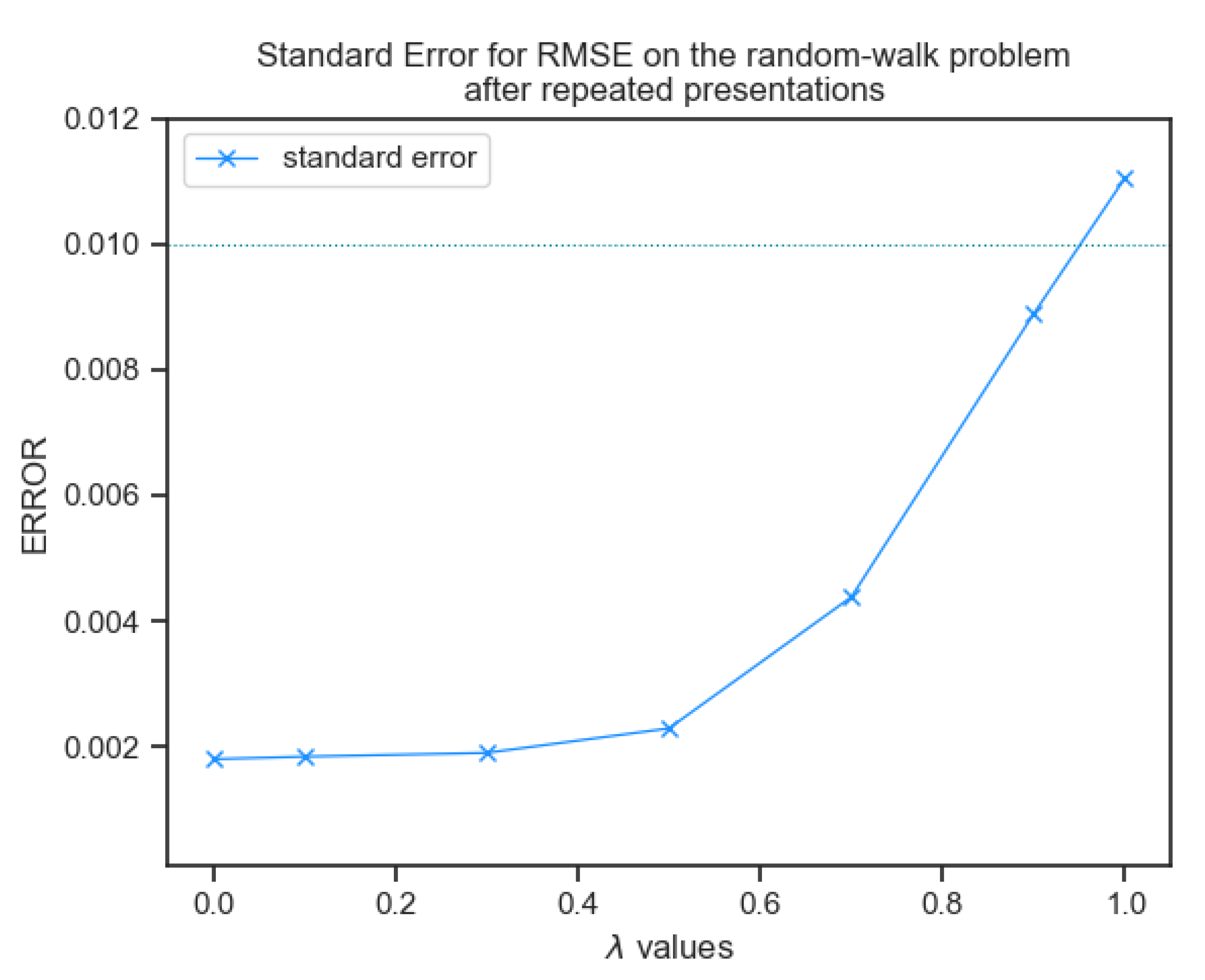
Figure 9.
Experiment 2 results – Sutton (left), reproduced with decay (middle) and without decay (right) for single presentation
Figure 9.
Experiment 2 results – Sutton (left), reproduced with decay (middle) and without decay (right) for single presentation
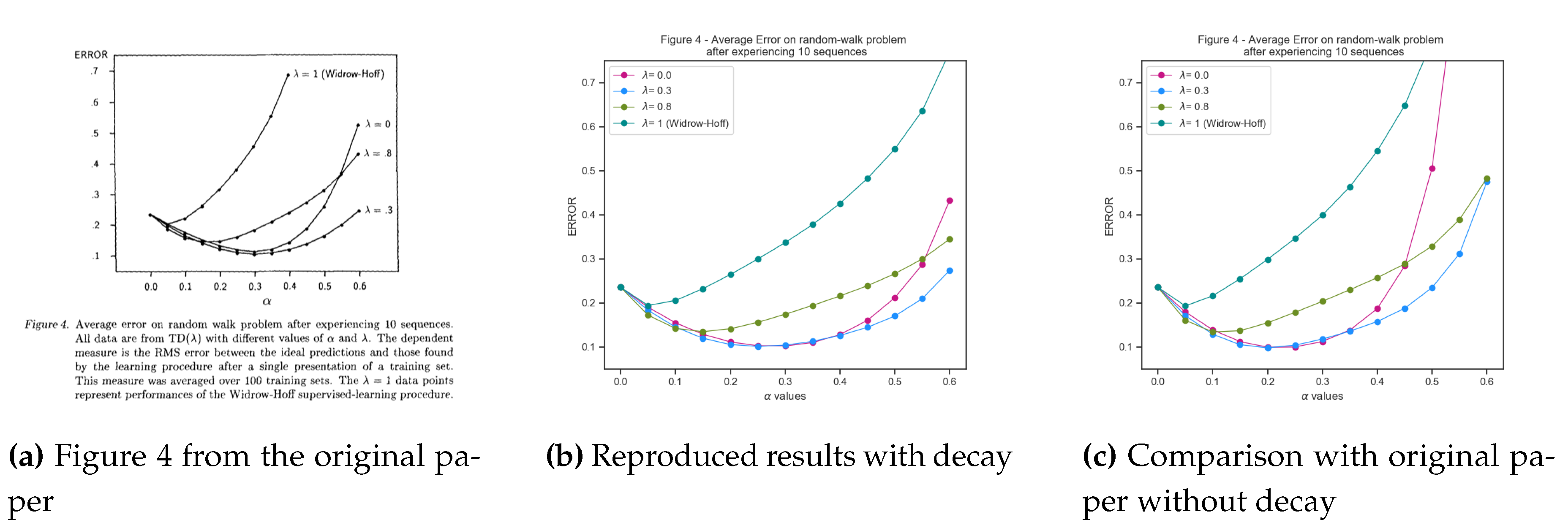
3.2. Experiment 2 - Learning Rate Analysis
The goal of the next experiment is to analyze the effects of learning rate () on TD learning algorithms and identify the appropriate learning rates for the each of the values being investigated. This would generate interesting insights on the learning rate effects and aid in determination of the best to solve this MRP.
3.2.1. Description and Implementation
For this experiment, the earlier procedure has been updated as follows. (1) Instead of "repeated presentations", each training set was presented only once i.e, "single presentation" (2) Weight updates accumulated over one sequence were updated after each random walk sequence itself, rather than at the end of each training set as convergence was not required as depicted in Figure (Figure 10). The experiment is conducted over a range of alpha () values and the weight vectors are initialized at 0.5 for each run to prevent any inductive bias, as the training sets are presented. Root mean squared (RMS) error was computed between the ideal values and the predicted values as described step-by-step in Algorithm (2)
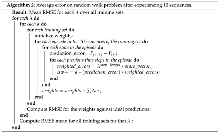
3.2.2. Results
As with the earlier experiment results, TD(1) continues to have the highest range of errors for all alpha () values and the learning rate () has a significant impact on the performance of the TD algorithm. Intermediate values between perform the best with the least error and also produces minimal error over a range of values. It is also worthy to note that TD(0) performs better than TD(1) as earlier but produces more error than the optimal values. This lends the intuition that for an MRP problem such as this 7-state random walk, the influence of the past predictions is necessary to some extent to drive towards the ideal prediction values faster.
3.2.3. Observations and Analysis
The results match closely with the original results for most of the values. Only the error rate for TD() does not rise at the rate represented in the original paper, though the difference in errors at between the paper and the reproduction results are minimal. For other values, the errors are close to the original paper, lending the argument that the difference in the values for might be due to the randomness of the training data set and different length of sequences generated for the original paper, allowing curve to accumulate more error than the training sets used for the reproduction results.
3.2.4. Parameter – Learning Rate Decay
A key distinction was added to the original algorithm for reproduction of the above experiment, in the form of a learning rate decay to generate plots closer to the original result. As noted in the paper [1] as part of the convergence proof, "if is reduced according to an appropriate schedule, then the variance converges to zero as well". Hence the experiment was conducted with a decay rate of 0.995 to perform updates lesser as the learning proceeds iterating over the training set. It is known for larger learning rate values, the weights will oscillate with a magnitude of and the TD error. The replicated experiment results without an alpha decay is provided for reference in Figure (Figure 9) and as expected, the errors increase at a higher rate, as continued learning happens throughout the training set. From these results, though not recorded it is evident that the original paper performed this experiment with a learning rate decay schedule.
3.2.5. Optimal Learning Rates
Using the experiment, the optimal learning rates for each of the values were determined. The interesting aspect of this observation was irrespective of decay usage, the optimal learning rates remain unchanged [see Table (Table 1)). This provides the intuition that for more complex MDPs, the learning rate might be determined as a hyper parameter for optimal performance.
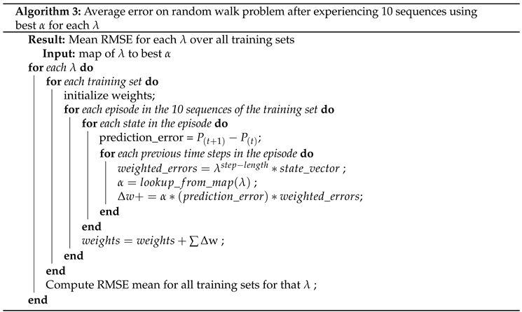
3.3. Experiment 3—TD() with Best Learning Rate ()
The goal for this final experiment was to prove the intuitions around TD(0) and TD() on how the optimal usually lies between 0 and 1 and the convergence of the TD learning methods at different to sub optimal values for the same training set for the given MRP. Weight updates were performed after each random walk sequence itself and the weight vectors are initialized at 0.5 similar to the previous experiment.
3.3.1. Description and Implementation
The previous experiment is repeated for a range of values using the best learning rate values (learning rate producing the lowest RMSE) for each identified. The training set data is presented only once and the mean RMSE is computed for the 100 training sets. Similar to the previous experiments, weight updates are performed after every sequence itself and the step-by-step procedure is available in Algorithm (3).
3.3.2. Results
Observing the RMSE for each , the earlier intuition of the best being around 0.3, is verified. TD(1) (Widrow-Hoff) results continue to exhibit the highest error values even at its best learning rate similar to the earlier experiments. Interestingly, for this Markov reward process, TD(0) has a slightly higher error rate than the optimal value, which might be attributed to the slowness of reward propagation in a typically long sequenced MRP such as the random walk. As noted in Table (Table 2) , when an observation-outcome pair of is used, the iteration update depicts the slowness of prediction propagation. In TD(0) only the weights of state F is updated, while in , both states E and F were updated enabling the procedure to learn faster. The TD(0) does perform better than the first experiment with lower RMSE at its best learning rate , however, has the least RMSE of all values. Note that this problem does not manifest with repeated presentations as the propagation happens eventually.
3.3.3. Observations and Analysis
The results match closely with the original paper results with having the lowest RMSE errors. Performing the experiment with a learning rate decay, generates results close to the ones without decay as the presentation of 10 sequences per training set, seems to converge to an optimum value as depicted in Figure (Figure 11). The comparative analysis with the paper results, show a slight variation for values 0 and 0.1 indicating that the training dataset from the original paper, gathered more error due to the slow prediction propagation in comparison to the training dataset used for reproduction. However, the rest of the results follow closely the paper results within a tolerance of less than 0.05. This minor differences are expected due to the randomness of the training data set used and also possibly due to different sequence run lengths being generated in the training data sets.
3.3.4. High RMSE in TD(1)
In spite of choosing the best suited learning rate , TD(1) still exhibits the highest RMSE, while an intermediate value of , performs with the least RMSE. Intuitively, the high error rate in TD(1) can be attributed to the dependency on the final outcome for calculating the predictions, rather than maximum likelihood estimates. An outcome-based approach such as TD(1) or Monte-Carlo methods rely on sufficient samples being available to converge to the global optimum values. Especially with limited training dataset, the effects of a less likely trajectory have a larger influence in TD(1) in comparison to with values lesser than 1. performs similar to the maximum likelihood estimate structure and base predictions on all available trajectories, rather than depending more on a less likely sample.
4. Additional Experiments
Two additional experiments (not performed in the original paper) were conducted. Training datasets with varying sizes of 50, 200 and 500 were generated, and repeated presentations was performed to observe any change as illustrated in Figure (Figure 12). The predictions across different episodes do not converge due to the stochasticity involved with the experience and rather oscillates around the expected values. However, the behaviour of TD for different values of remain consistent with the earlier findings.
The second experiment was conducted by limiting the length of a walk sequence for different values and under "repeated presentations" exhibited very similar behaviour as the previous experiment of varying training data sizes. The values again fluctuate around the previous experiment results but demonstrate the same behaviour for different values as discussed above and illustrated in Figure (Figure 13).
5. Conclusion
As the original paper concludes, TD learning provides a great framework model to predict future values incrementally based on observed measurements and actions. Such temporal predication problems are multi-step and TD learning is well suited to provide such predictions with high fidelity. TD(1) has proven to be a cheaper and faster alternative to supervised learning while provides an optimal prediction method for finite training datasets, using "repeated presentations".
A key problem with TD learning rises from the bootstrapping process, creating high bias for predictions based on the initial conditions. Though with infinite samples, the bias gets reduced, they can still cause significant instability if used on problems with "deadly-triad" [3] of value function approximation, bootstrapping and off-policy learning. Recent papers have shown usage of experience replay and other methods that work around the deadly triad restriction. The above experiments demonstrate that TD learning astutely captures the negative impact of a state accurately and utilizes that information to determine the outcome, effectively eliminating other noise possibly contributed by optimistic sequences etc., Though, there are niche hand-crafted MDPs that are capable of posing more difficulty to TD learning as described in the paper, most common problems are always benefitted by the usage of TD learning. The paper discusses few semantic cases that could be constructed which fails with TD, but for most common temporal problems, they perform admirably better. With the surge of temporal and credit assignment problems, reinforcement learning algorithms are found to be best suited to solve such domains and TD performs extremely well with incremental computation and lesser memory as would be demonstrated in the later portions of the paper.
References
- Sutton, R.S. Learning to predict by the methods of temporal differences. Machine learning 1988, 3, 9–44. [Google Scholar] [CrossRef]
- Dietterich, T.G.; Michalski, R.S. Learning to predict sequences. Machine Learning: An Artificial Intelligeve Approach 1986, 11, 63–106. [Google Scholar]
- Sutton, R.S.; Barto, A.G. Reinforcement learning: An introduction; MIT press, 2018. [Google Scholar]
- Chung, K.L. Markov chains; Springer-Verlag: New York, 1967. [Google Scholar]
Figure 1.
TD(0) learning convergence over episodes
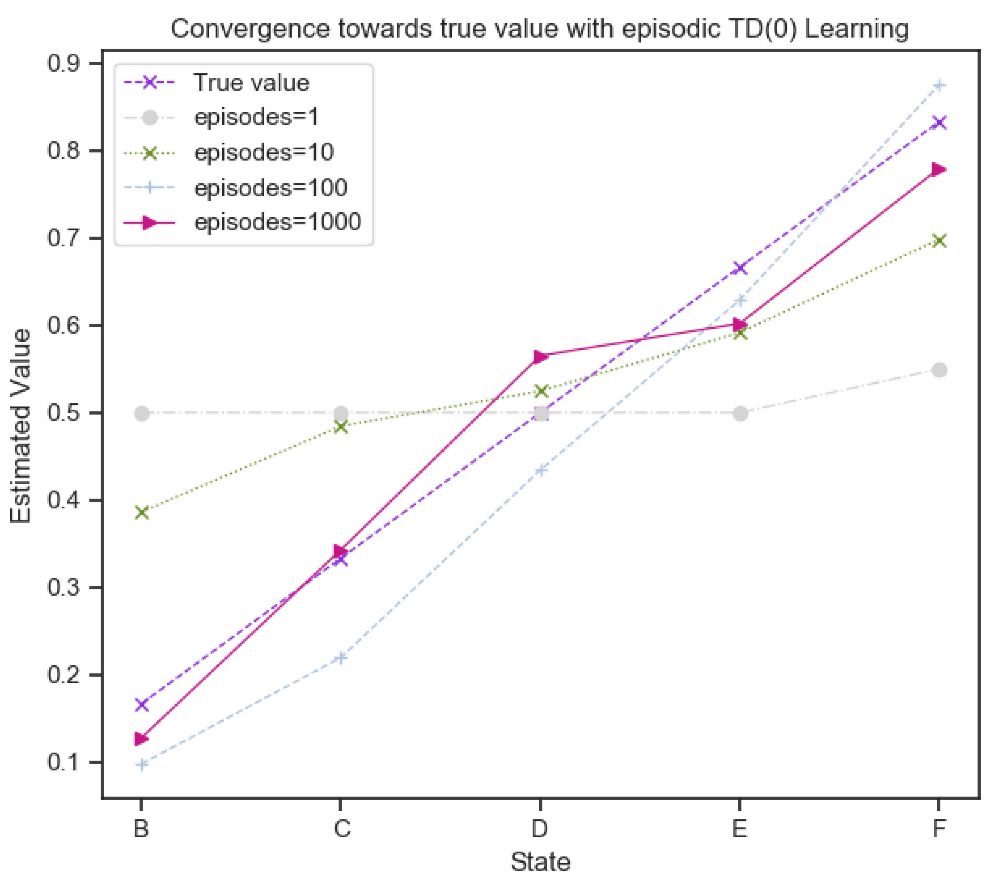
Figure 2.
Seven state random walk
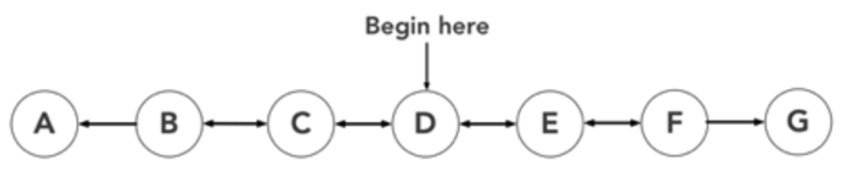
Figure 3.
Unit vector representation of simple sequence
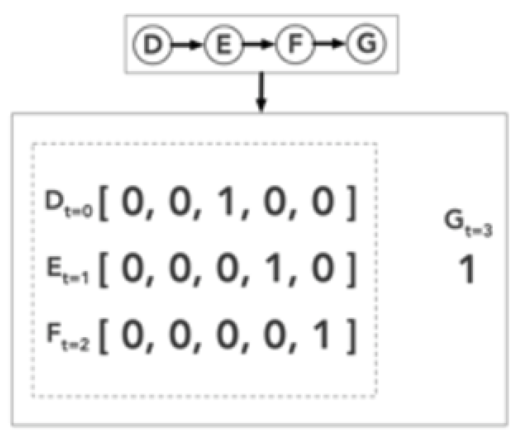
Figure 4.
Representation of the 100 training sets & 10 sequences each
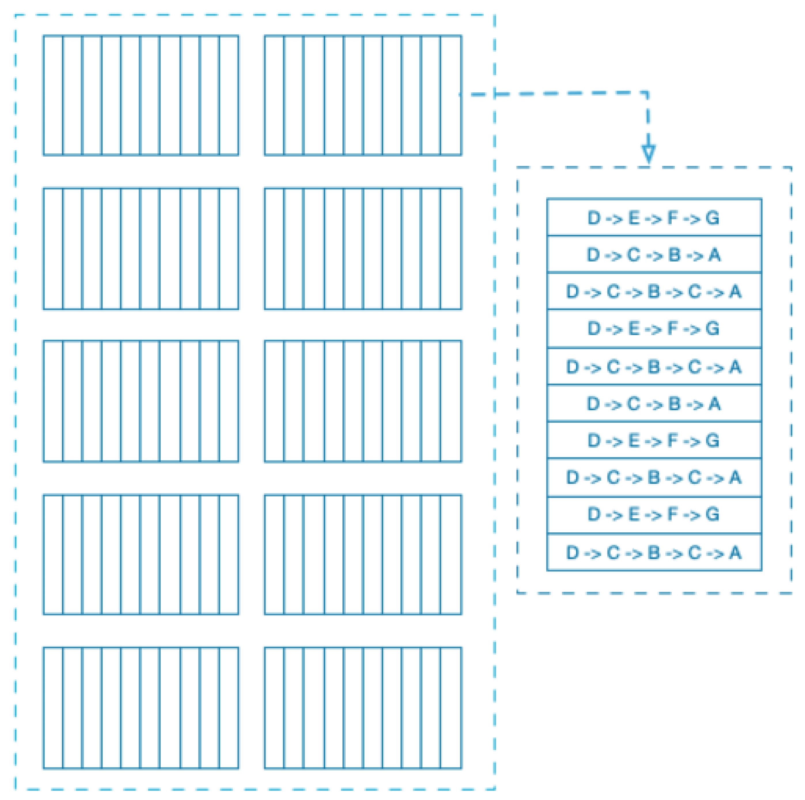
Figure 5.
Weight accumulation and update after each training set
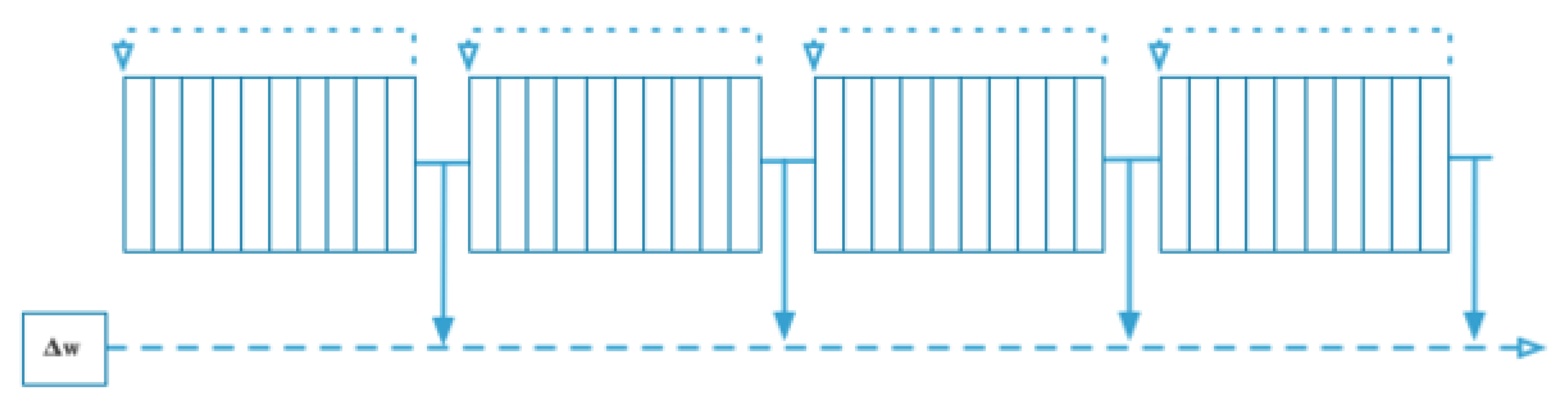
Figure 6.
Repeated presentations result – Reproduced (middle), Sutton (left) and their comparison along with decay (right)
Figure 6.
Repeated presentations result – Reproduced (middle), Sutton (left) and their comparison along with decay (right)
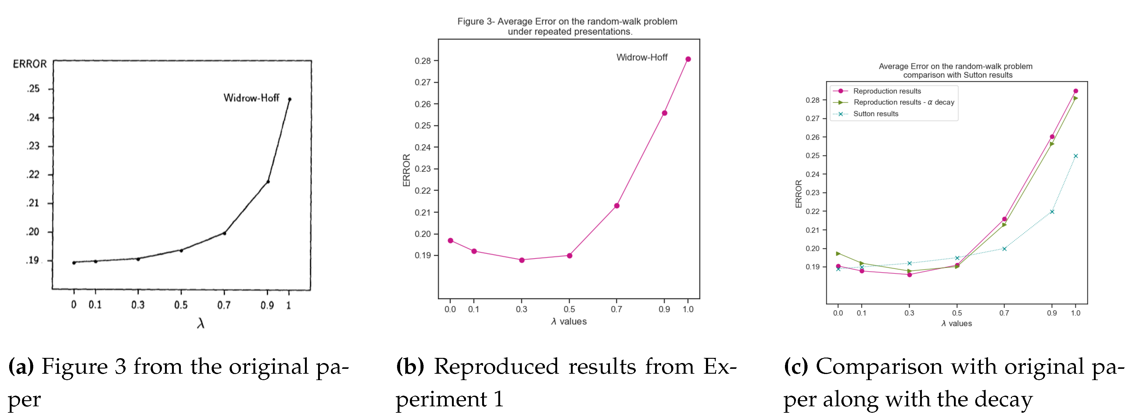
Figure 7.
Effect of different values in TD(0) learning
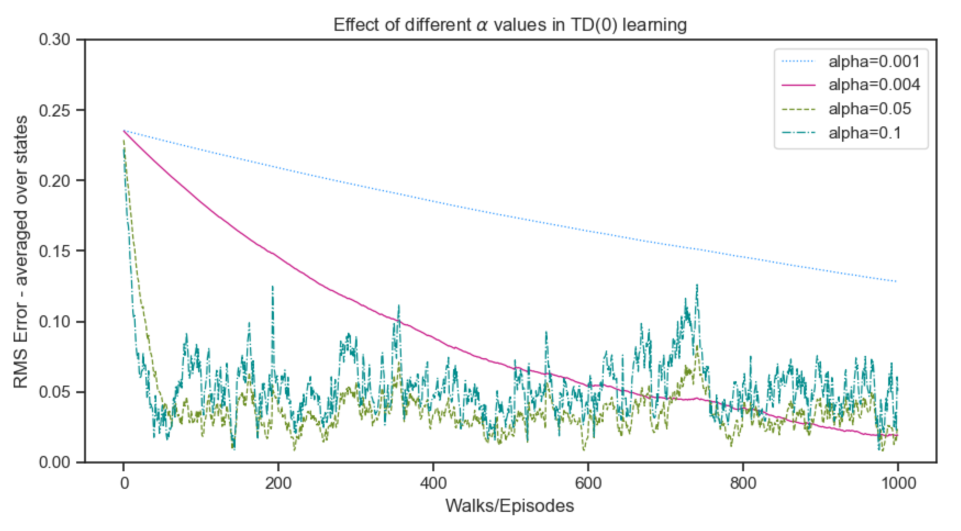
Figure 10.
Weight updates after each sequence
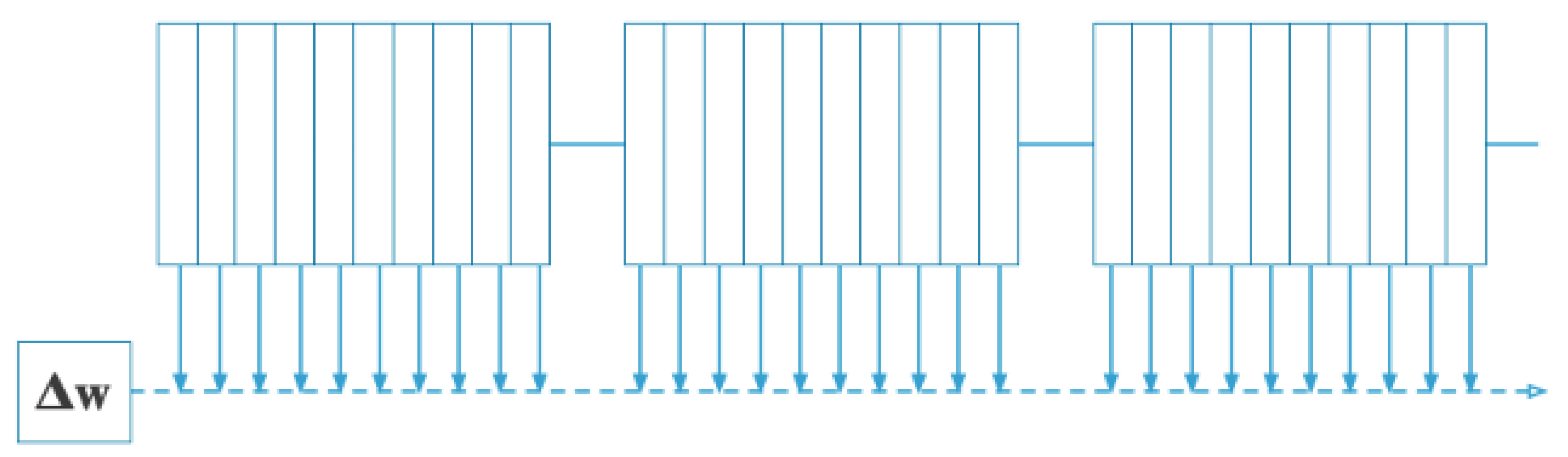
Figure 11.
Single presentation result with best values for each - Sutton (left), Reproduced (middle), and their comparison along with decay (right)
Figure 11.
Single presentation result with best values for each - Sutton (left), Reproduced (middle), and their comparison along with decay (right)
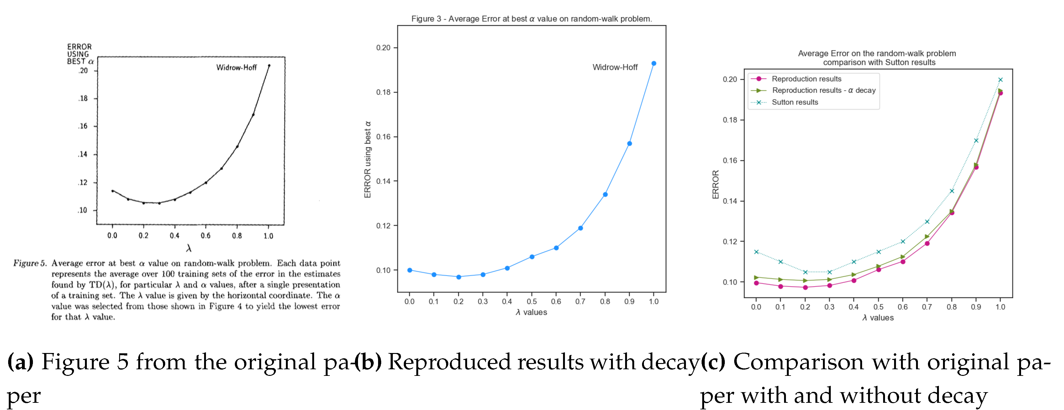
Figure 12.
Repeated presentations for different training sizes
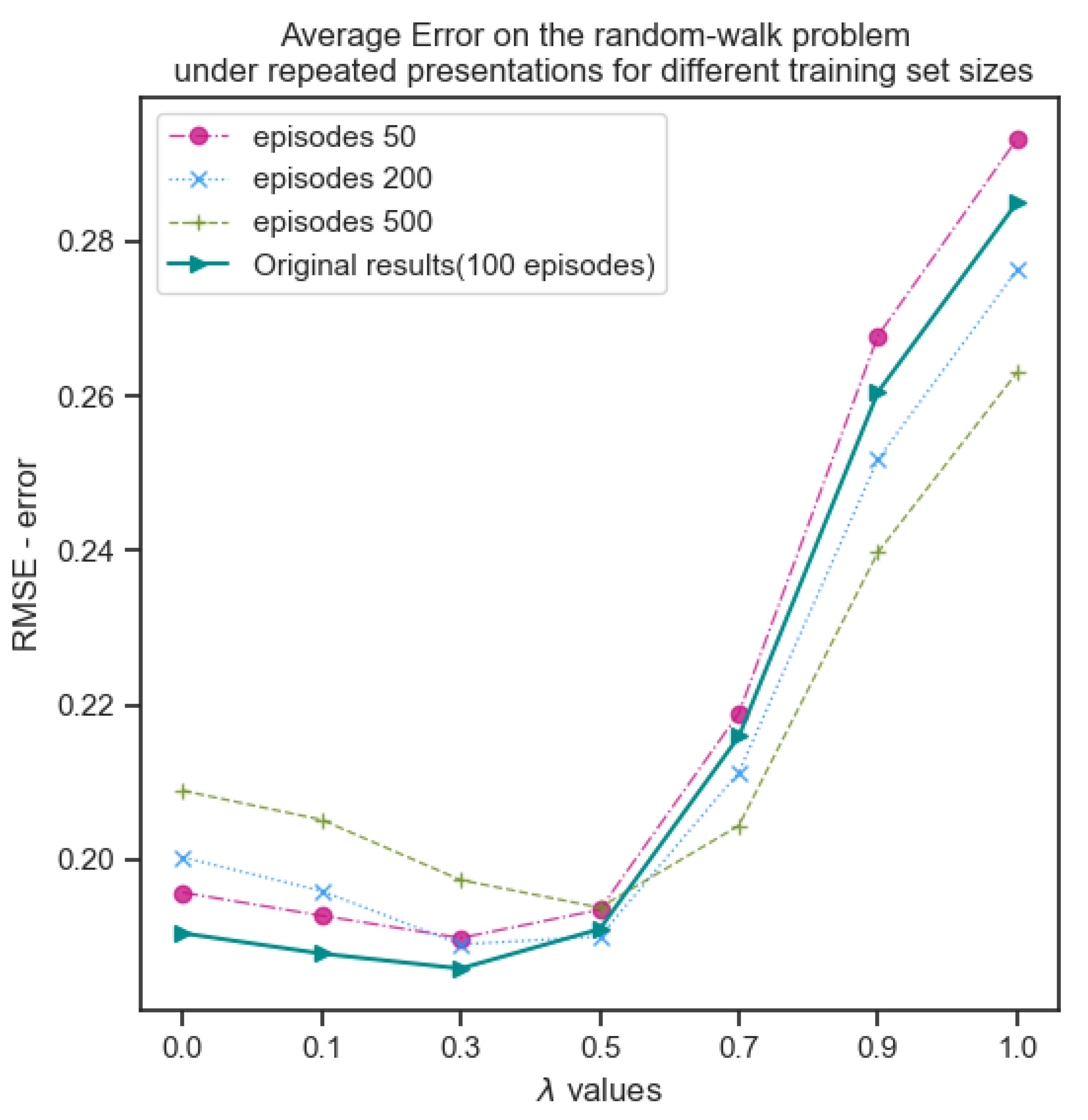
Figure 13.
Repeated presentations for different episode lengths
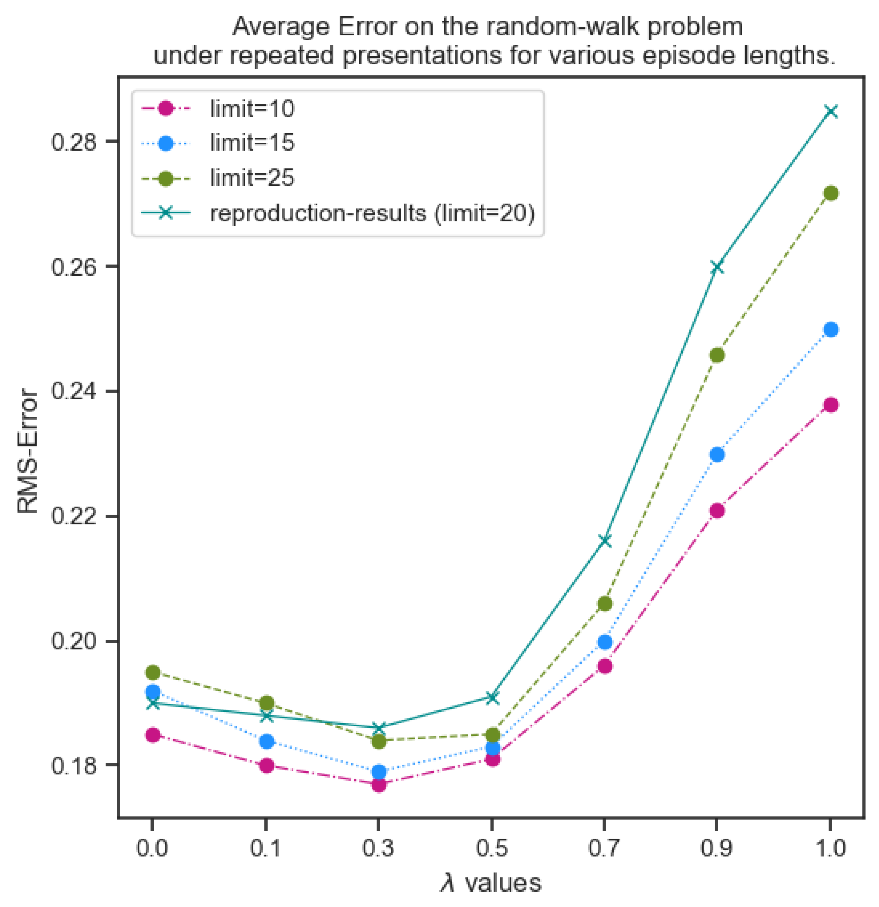

Table 1.
Best value for each
| 0.0 | 0.1 | 0.3 | 0.5 | 0.7 | 0.9 | 1.0 | |
|---|---|---|---|---|---|---|---|
| 0.20 | 0.20 | 0.20 | 0.15 | 0.15 | 0.10 | 0.05 |
Table 2.
TD(0) and TD(=0.3) update on the first iteration
| α = 0.1 | TD(0) | TD(0.3) |
|---|---|---|
| Iteration = 0 | [0.50, 0.50, 0.50, 0.50, 0.50] | [0.50, 0.50, 0.50, 0.50, 0.50] |
| Iteration = 1 | [0.50, 0.50, 0.50, 0.50, 0.55] | [0.50, 0.50, 0.50, 0.52, 0.55] |
Disclaimer/Publisher’s Note: The statements, opinions and data contained in all publications are solely those of the individual author(s) and contributor(s) and not of MDPI and/or the editor(s). MDPI and/or the editor(s) disclaim responsibility for any injury to people or property resulting from any ideas, methods, instructions or products referred to in the content. |
© 2024 by the authors. Licensee MDPI, Basel, Switzerland. This article is an open access article distributed under the terms and conditions of the Creative Commons Attribution (CC BY) license (http://creativecommons.org/licenses/by/4.0/).
Copyright: This open access article is published under a Creative Commons CC BY 4.0 license, which permit the free download, distribution, and reuse, provided that the author and preprint are cited in any reuse.


