Preprint
Article

Relations of Society Concepts and Religions from Wikipedia Networks

Altmetrics

Downloads

12

Views

12

Comments

0

This version is not peer-reviewed

Submitted:

04 December 2024

Posted:

05 December 2024

You are already at the latest version

Alerts
Abstract

We analyze the Google matrix of directed networks of Wikipedia articles related to 8 recent Wikipedia language editions representing different cultures (English, Arabic, German, Spanish, French, Italian, Russian, Chinese). Using the reduced Google matrix algorithm we determine relations and interactions of 23 society concepts and 17 religions represented by their respective articles for each of the 8 editions. The effective Markov transitions are found to be more intense inside the two blocks of society concepts and religions while transitions between the blocks are significantly reduced. We establish 5 poles of influence for society concepts (Law, Society, Communism, Liberalism, Capitalism) as well as 5 poles for religions (Christianity, Islam, Buddhism, Hinduism, Chinese folk religion) and determine how they affect other entries. We compute inter edition correlations for different key quantities providing a quantitative analysis of the differences or the proximity of views of the 8 cultures with respect to the selected society concepts and religions.

Keywords: 
Subject: Social Sciences  -   Ethnic and Cultural Studies

1. Introduction

During human society evolution several concepts of society have been developed. Their relations and interactions are studied by social sciences as discussed for example in [1,2]. Among these concepts there are those linked to social society structure, as e.g. law, education, culture; political formations as e.g. capitalism, socialism, communism and others. These concepts represent social concepts of society. Other concepts are represented by religions which play an important role in human society formation. This role and relations of religions and human societies have been studied and investigated from various view points including history, philosophy, psychology, archaeology, economy and other sciences (see e.g. [3,4,5,6,7,8,9] and Refs. therein). However, the mathematical analysis of these relations is essentially absent since it is rather difficult to use and apply rigorous mathematical methods to human sciences and religions. In this work, we try to develop a mathematical framework to investigate religions and society concepts relations based on the Wikipedia network analysis. We consider a directed network composed of Wikipedia articles (nodes) with generated hyperlinks (citations) between them. Already two decades ago the free online Wikipedia has superseded old encyclopedias such as Encyclopedia Britannica [10] in quality and volume of articles related to scientific topics [11]. At present the academic analysis of information contained in Wikipedia finds more and more applications as reviewed and described in [12,13,14,15,16]. Thus Wikipedia contains an enormous diverse database of human knowledge which we use to determine relations of religions and society concepts obtained on purely mathematical grounds. Of course, religions are also human concepts related to society but for clarity we consider two groups of concepts formed by society: society social concepts and religions.
We analyze Wikipedia networks of different language editions by the Google matrix approach and Page Rank algorithm, originally developed and applied by Brain and Page for the World Wide Web search analysis [17,18]. We also use additional algorithms such as CheiRank [19,20,21] and the reduced Google matrix (REGOMAX) [22]. Various applications of these algorithms with an analysis of the importance and interactions of various Wikipedia articles and groups of articles have been reported for historical figures [20,23], world universities [20,24], politicians [22], banks and world countries [25] and other examples. The REGOMAX algorithm is particularly useful since it allows to determine effective interactions between nodes of a selected group taking into account direct and all indirect pathways between these nodes via the global network with a size exceeding by orders of magnitude the number of selected group nodes. These tools have been shown to operate efficiently not only for Wikipedia networks but also for the world trade network of UN COMTRADE [26] and the MetaCore network of protein-protein interactions [27].
In this work, we focus on the directed networks obtained from 8 actual Wikipedia language editions: English (EN), Arab (AR), German (DE), Spanish (ES), French (FR), Italian (IT), Russian (RU), Chinese (ZH). We consider that these 8 networks describe 8 different cultures since a language is one of the most important elements of culture. The 8 networks are generated from Wikipedia edition dumps of 1 October 2024 and the main network parameters are given in Table 1.
For our analysis we select from Wikipedia 40 articles about human concepts composed of 23 society concepts and 17 religions (and branches of religions) given in Table 2. These 40 concepts are analyzed for each of 8 Wikipedia edition networks. We show that the REGOMAX algorithm allows to determine nontrivial interactions among the 23 selected society concepts, 17 religions and also relations between these two groups for each of the 8 networks of Table 1. Furthermore, the obtained results also allow to characterize quantitatively the correlations between these 8 cultures.
The paper is composed as follows: in Section 2, we present some technical details about the used data sets and in Section 3 the used mathematical tools for network and correlation analysis are briefly reviewed. Section 4 presents and provides a detailed discussion of our results and Section 5 provides the final discussion and conclusion.
Additional materiel, additional figures and data files are available at [28].

2. Data Sets of Wikipedia Networks

2.1. Construction of the Wikipedia Networks

To construct the Wikipedia networks for the different language editions of Table 1, we downloaded the official xml-dump files for each edition (versions with all pages and articles in a single file) with time stamp of October 1, 2024. First, we extracted for a given edition the titles of all main content articles with namespace key value being 0 thus excluding technical Wikipedia articles of type Category, Help, File, Wikemedia etc. having other namespace key values. Also titles corresponding to a redirection to another existing article were not taken into account. This procedure provides the list of all article titles/network nodes with a technical index given by the initial order of the xml-dump file which is typically roughly alphabetical (but not exactly). This technical initial index, while being important to store the network links and for the different computation codes, will not be used in this work to characterize specific articles/nodes. Instead, we will use the PageRank index K M (see below) to characterize different nodes.
In a second step, we determined for each article the links to other articles in the same Wikipedia edition. These links are (with some technical complications) available in the xml-dump files as clear text article titles but sometimes it is necessary to capitalize the first character of a link name to identify the proper article title, which is always capitalized for the first character, and the corresponding node index. This capitalization procedure is for accented or special characters (with multibyte utf8 codes), e.g. in the case of French or Russian article titles, a technical nontrivial operation for which we used the library Utf8proc [29]. Links to redirection titles, outside webpages or other wikipedia editions were not taken into account. Multiple links between two articles, in particular several links pointing to a particular position inside the target article, were counted as a single unique link. Links from an article to itself were kept but also only as a single link.
In this way, we obtained the Wikipedia networks with full “official” lists of article titles for the 8 editions and tables of links, with some key values shown in Table 1, e.g. with typical node numbers between N 6.9 × 10 6 (for the English Wikipedia edition EN) and N 1.2 × 10 6 (for the Arabic Wikipedia edition AR) and typical link numbers between N 1.9 × 10 8 (EN) and N 1.6 × 10 7 (AR). The ratio N / N between both has typical values 13-27. Table 1 also shows the number of dangling nodes N d corresponding to nodes having no outgoing link to another Wikipedia article of the same edition. These nodes require special treatment in the Google matrix approach (see next section) and the typical values are N d 10 3 - 10 5 which represents a very small fraction of the full number of nodes N 10 6 - 10 7 .

2.2. Edition Specific Subsets

Starting with English Wikipedia, we select a group of 40 articles about 23 society concepts and 17 religions (or branches of religions) shown in Table 2. The order of these articles is fixed by first PageRank ordering the 23 society nodes and then the 17 religion nodes providing the group index K g . Then for each of the other editions, we determine an equivalent group using the official Wikipedia links between two different editions. For this we downloaded the source html files of the 40 EN-articles and extracted from these files the corresponding article titles of the other editions. This information is indeed contained in these source files in the other language submenu where the corresponding articles in other language editions can be selected from a given English Wikipedia page. It turns out that for all the other 7 language editions and each of the 40 EN-articles of Table 2, we were able to find the corresponding article associated to the other edition (for some other language Wikipedia editions, not used in this work here, the number of found “translated” articles may be less than 40).
We note that this procedure is important and that simple linguistic title translation may lead to wrong articles in the other edition. For example the EN-article “Society” ( K g = 15 in Table 2) translates linguistically to “Gesellschaft” in German but the DE-article “Gesellschaft” corresponds more to a technical article with links to several other DE-articles using the word “Gesellschaft” in the title and for different contexts (e.g. sociology, ethonology, state-law etc.). However, the official inter edition Wikipedia link from the EN-article “Society” to the DE-Wikipedia edition provides the title “Gesellschaft (Soziologie)” which is a different DE-Wikipedia article than “Gesellschaft”. There are some other similar examples like this, also for FR-Wikipedia. In particular both articles about the Orthodox Church with very specific differences between them (with K g = 29 , 40 in Table 2), require to use the official inter edition Wikipedia links while simple linguistic translation may easily lead to the wrong article.
In this work, we will for convenience always use (in Tables and Figures below) the English article titles given in Table 2, even when we speak about another edition. Of course, the network index values of the 40 group nodes, necessary for the computation of the reduced Google matrix (see below), were correctly determined individually for each edition using the properly translated group list for the same edition, eventually using article titles in special character sets (especially for AR, RU, ZH).
In Table 3, we summarize the group local PageRank and CheiRank indices K and K * (see next section) for all 40 subset nodes and all 8 Wikipedia editions of Table 1 and using for each edition the properly translated group for this edition as described above.

3. Google Matrix Algorithms

3.1. Google Matrix Construction

We construct the Google matrix G of the different Wikipedia networks with N nodes (articles) in the usual way [17,18,21]. First, we define the adjacency matrix A by A i j = 1 if node j points to node i (if there is a link from the Wikipedia article j to the article i) and A i j = 0 otherwise. Then the stochastic matrix S of Markov transitions if defined by S i j = A i j / l A l j for columns j with l A l j > 0 . For dangling nodes j, having no outgoing links, i. e. with l A l j = 0 , we simply define S i j = 1 / N for all values of i. The columns of S are sum normalized, i. e. l S l j = 1 , and conserve the total probability when the matrix S is multiplied to an arbitrary probability vector P, i. e. i P ˜ ( i ) = i P ( i ) = 1 if P ˜ = S P .
Finally, the Google matrix elements are defined as
G i j = α S i j + ( 1 α ) / N
where 0.5 α < 1 is the damping factor for which we choose the usual standard value α = 0.85 [18,21]. The columns of G are also column sum normalized and it also conserves the probability in the same way as the matrix S.
Physically, this matrix describes a stochastic process where a random surfer jumps over the network. With a probability α the surfer jumps randomly from his actual page j to a random page page i among the pages with existing links j i and with a complementary probability 1 α he jumps to an arbitrary random node of the network. For dangling nodes he jumps immediately to an arbitrary random node. The damping factor allows to connect all isolated communities and avoids that the random surfer is trapped inside a small finite subset of nodes with no links going outside to this subset.

3.2. PageRank, CheiRank

Due to the damping factor the stochastic process defined by G converges, according to the Perron-Frobenius theorem, in the long time limit to a stationary probability P = lim t G t P 0 where P 0 is an arbitrary initial probability vector (with real values, P 0 ( i ) 0 , i P 0 ( i ) = 1 and the same holds also for the stationary limit P ( i ) ). The stationary vector P, in the following also called PageRank vector, satisfies the eigenvalue equation G P = λ P = P with the maximal eigenvalue λ = 1 of G. One can show from (1) that all other (real or complex) eigenvalues λ of G satisfy the inequality | λ | α providing a spectral gap 1 α ensuring the exponential convergence to the steady state vector and the iteration G t P 0 indeed provides a reliable numerical method to compute the PageRank.
The value of the PageRank component P ( i ) represents the importance of the node i which is essentially proportional to the number of all ingoing links j i [18] but also weighted with the importance P ( j ) of the source nodes j. It is also useful to determine the rank index K M ( i ) = 1 , 2 , 3 , of a node i by ordering the nodes i with decreasing values of P ( i ) . This index is also called PageRank index such that K M ( i ) = 1 for maximal P ( i ) , K M ( i ) = N for minimal P ( i ) and more generally K M ( i ) < K M ( j ) corresponding to P ( i ) > P ( j ) . The Google search engine actually uses this PageRank index to select the presentation order of search results which typically result in rather long lists of web pages.
Following [19,20], we can also consider the network obtained by the inversion of all the directions of links of the original network with a resulting Google matrix noted G * (which is different from the simple transpose G T due to different column-sum normalizations and different sets of dangling nodes). The PageRank vector associated to G * is called CheiRank vector and noted P * with a CheiRank ordering index K M * ( i ) . The value of P * ( i ) is typically proportional to the number of outgoing links i j with some weight factors being P * ( j ) .
It is also useful to introduce a 2DRank index K 2 which orders nodes on the PageRank-CheiRank plane by order of their appearance in a square of increasing size K M = K M * starting from K M = K M * = 1 (see details in [20]). The coarse grained density of the distribution of nodes in the K M - K M * plane, eventually in log-scale, provides also a useful graphical presentation of the network nodes; see also Figure 1 and Figure 2 below.
In this work, we note by K M ( K M * ) the PageRank index for the full (inverted) network while K ( K * ) denotes a reduced limited index for the group(s) of 40 nodes corresponding to Table 2 and Table 3, i. e. with values K = 1 , , 40 ( K * = 1 , , 40 ). These local group indices K and K * can be computed by different methods, e.g. by direct extraction from K M and K M * by attributing the values of K ( K * ) with increasing values of K M ( K M * ), e.g. K = 1 for the subset node with minimal K M value, K = 2 for the subset node with the second minimal K M value etc. We used however a slightly different method which consists simply of reducing the PageRank vector to the subset, with new index values being 1 , , 40 , and then computing K by ordering the components of this reduced (or projected) PageRank vector (and similarly for K * using a reduced CheiRank vector). A third, more complicated method is to compute the projected PageRank from the reduced Google (see next section). Table 3 summarizes these local indices K and K * for the 8 editions and their associated subsets of 40 nodes.

3.3. Reduced Google Matrix

In [22] a method and algorithm (REGOMAX) was introduced to define and compute a reduced Google matrix for a selected subset of N r nodes (with N r 10 2 - 10 3 being typically of modest size) taking into account both direct links between two nodes of this subset and also indirect links between two such nodes using pathways along nodes outside this subset. We note that the contributions of indirect links are very important and their omission may lead to erroneous results as it was demonstrated in [23] for a directed network of historical figures of Wikipedia previously studied in [30].
For this approach it is convenient to write the Google matrix G and the PageRank vector P of the global network as
G = G rr G rs G sr G ss , P = P r P s
where the label “ r ” refers to the nodes of the reduced network of N r subset nodes, and “ s ” to the other N s = N N r nodes which form the complementary network acting as an effective “scattering network”. The PageRank eigenvalue equation G P = P implies [22] that the projected PageRank P r can be computed from
G R P r = P r
where the reduced Gooogle matrix of size N r × N r is given by
G R = G rr + G rs ( 1 G ss ) 1 G sr = G rr + G pr + G qr .
This matrix is also a stochastic matrix with columns being sum normalized. For practical reasons, we renormalize P r such that j P r ( j ) = 1 where the sum runs over all nodes of the small subset. In (4), the first term G rr accounts for all direct links between two nodes A and C in the subset and the second term represents all indirect links between these two nodes using a chain of links from A to B 1 , then from B 1 to B 2 , , and then from B m to C where the intermediate nodes B 1 , , B m belong to the complementary scattering network of N s nodes. Such a pathway corresponds to the term G rs G ss m G sr obtained by expanding the above matrix inverse in a geometric series over such terms. We note that the matrix G ss has a leading eigenvalue λ c close to 1 but smaller than 1 (if N r > 0 ) such that the matrix inverse is well defined. The second term can be furthermore decomposed [22] in two contributions G pr + G qr where G pr is a rank-1 matrix obtained by extracting from the matrix inverse the contribution of the leading eigenvector of G ss (which is rather close to P s ) and G qr is the remaining contribution which can be numerically efficiently computed by a rapid convergent geometric series over a certain specific matrix obtained from G ss by a projection on the space bi-orthogonal to the leading eigenvector of G ss (see [22] for details). Initially, this decomposition was introduced to find an efficient numerical algorithm to G R but it turns out that it also useful in terms of interpretation. The term G pr , while having a dominant weight, has a very simple structure with nearly identical columns being close to P r (all columns are proportional with factors close to 1). This term is essentially determined by the leading eigenvector of G ss (see [22] for an explicit formula).
Due to the simple structure of G pr it is the other matrix G qr , smaller in numerical weight, which represents the most nontrivial information related to indirect hidden transitions. We also define the matrix G qr ( nd ) which is obtained from G qr with its diagonal elements being replaced by zero. We note that each component can be characterized by its weight being W R , W pr , W rr , W qr ( W qr ( nd ) ) for G R , G pr , G rr , G qr ( G qr ( nd ) ) respectively and which is defined as the sum of all matrix elements divided by its size N r . (Since G R is also column sum normalized we always have W R = 1 .) Studies for examples of reduced Google matrices associated to various directed networks can be found in [22,24,25,26,27].
We note that the first equivalence relation in (4) is similar to the Schur complement in linear algebra (see e.g. [31]). Issai Schur introduced the Schur complement in 1917 (see history in [31]) and later it found a variety of applications [31,32]. However, the expansion in the form of three matrix components, given by the second equivalence relation in (4), with the physical sense of each component was introduced only in [22].
In this work, we apply the reduce Google matrix approach to the group(s) of 40 Wikipedia articles shown in Table 2 and Table 3 and introduced in the last section. For all these cases we computed the reduced Google matrix and its different components, as well as the reduced PageRank vector P r and the group local PageRank index K (with values K = 1 , , 40 ). The same can also be done for the inverted network with Google matrix G * . However, in this work we present only results for the reduced Google matrix associated to G and not to G * (except for the local index K * which can also be obtained more directly by extraction from K M * or by ordering P r * which is defined in a similar way as P r ).
We present the positions of 40 articles in the PageRank-CheiRank plane for all 8 editions in Figure 1 and Figure 2; the reduced Google matrix and its components in Figure 3, Figure 4, Figure 5, Figure 6, Figure 7, Figure 8, Figure 9, Figure 10, Figure 11, Figure 12, Figure 13, Figure 14 and Figure 15 for all 8 editions.

3.4. Inter Edition Correlator Quantities

It is interesting to compare the different quantities we compute, such as P r , K, G R etc., between the different Wikipedia editions of Table 1. For this we consider different types of correlators for which we give a brief review below.
For example for two given data sets X i and Y i of size n s with i = 1 , , n s the Pearson correlation coefficient is defined as [33]
ρ X Y = ( X X ) ( Y Y ) σ X σ Y = X Y X Y σ X σ Y
where f ( X , Y ) = i f ( X i , Y i ) / n s is the average over an arbitrary function f ( X , Y ) and σ X = X 2 X 2 , σ Y = Y 2 Y 2 is the standard deviation of X and Y respectively. For ρ X Y > 0 ( ρ X Y < 0 ) one can state (for a given index i) that it is more likely that Y i > Y ( Y i < Y ) if X i > X . In other words deviations from the average values for X and Y have probably the same (opposite) sign if ρ X Y > 0 ( ρ X Y < 0 ).
The Kendall rank correlation coefficient is defined as [34]
τ X Y = 2 n c n p 1
where n p = n s ( n s 1 ) / 2 is the number of all possible pairs ( X i , Y i ) , ( X j , Y j ) with i < j and n c is the number of concordant pairs such that either X i < X j and Y i < Y j or X i > X j and Y i > Y j (same sorting order between the pair). Here, we have τ X Y = 1 ( τ X Y = 1 ) if both data sets have the same (reverse) sorting order.
In the (end of the) next section and in Figure 16, we present and discuss results for both correlators ρ q ( i ) q ( j ) and τ q ( i ) q ( j ) as 8 × 8 matrices where i , j = 1 , , 8 represent index values for the 8 Wikipedia editions and q ( i ) a data set/quantity computed for the given Wikipedia edition with index value i. Concerning the correlator (5), we consider five quantities q ( i ) being the reduced PageRank vector P r (all vector coefficients with n s = 40 ), the reduced Google matrix G R (all matrix elements with n s = 40 2 ), the religion or society sub-block of G rr + G qr ( nd ) (all sub-block matrix elements with n s = 17 2 or n s = 23 2 respectively) and also the local PageRank index K (all K values with n s = 40 ). For K we also compute the Kendall rank correlator (6) which is actually equivalent to the Kendall rank correlator for P r since the local ranking index K is obtained by ordering the values of P r , i. e. two K vectors for two different editions have the exact same number of concordant pairs as the related two P r vectors. We mention that mathematically both correlator quantities can take in theory values between 1 (perfect anti-correlation) and + 1 (perfect correlation) while values close to 0 indicate small or absent correlations. However, for the 6 correlator quantities mentioned above only positive correlator values appear (actually with minimal values above 0.33 ; see Figure 16 for more details).

4. Results

4.1. Article Location on PageRank-CheiRank Plane

We first discuss some results for the local ranking indices K and K * given in Table 3 for the 8 edition cases and the 40 edition specific selected articles. Concerning EN-Wikipedia, we note that the top 6 PageRank positions in the subset of Table 2 are taken by religions with Catholic Church at K = 1 while the first society concept Law only appears at K = 7 . This tendency is preserved in the other 7 editions where religions still take the top 3-4 PageRank positions while such a society concept as Liberalism only appears at K = 5 for the AR, ES, FR, IT editions. There are two exceptions being Nazism at K = 2 for DE, that is clearly linked to German history, and surprisingly also for ZH where the top society concept is Law at K = 3 being significantly above Communism at K = 13 . For EN the top society concept is also Law at K = 7 and for RU it is Economy at K = 7 .
Among religions the top K = 1 position is taken by Catholic Church for EN, DE, ES, IT and Christianity is at K = 1 for FR, ZH (Buddhism is at K = 2 for ZH). Somewhat surprisingly for RU Islam is at the top PageRank position K = 1 and Christianity is at K = 2 . This is probably related to a significant Muslim population in Russia that is however significantly smaller than its christian population. Islam is the top religion for the AR-Wikipedia edition which appears to be rather natural. However, here Christianity and Catholic Church appear at K = 2 and K = 3 respectively.
Concerning the CheiRank index K * , that characterizes the communicative properties of a node, the situation is more mixed. Thus we have at K * = 1 : Jainism for EN; Christianity for AR; Islam for DE, Anarchism for ES, FR; Catholic Church for IT; Monarchy for RU; Communism for ZH. We attribute such a mixing to stronger fluctuations of outgoing links as discussed in [21].
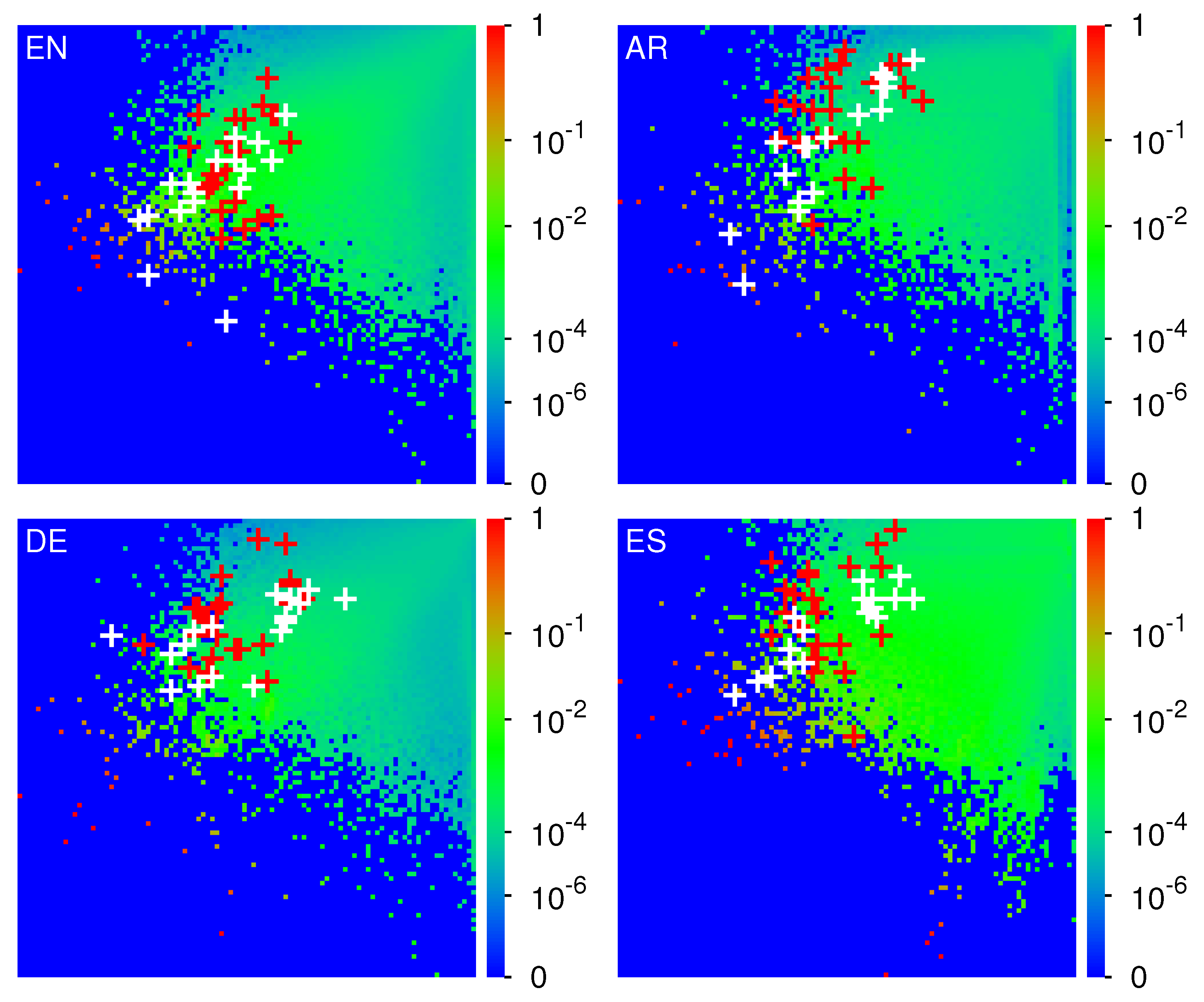
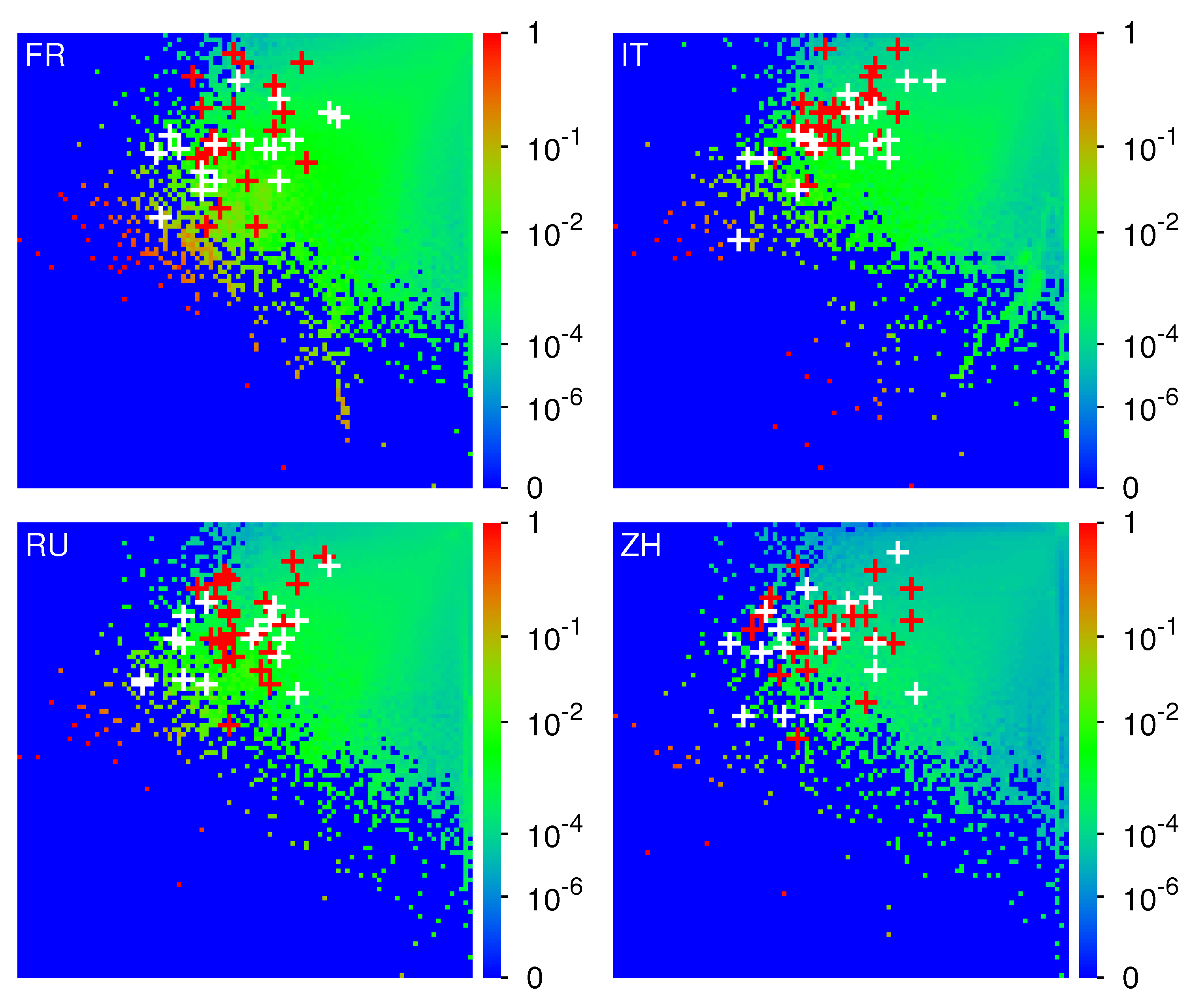
Concerning the global ranking indices K M and K M * for the full network, we show the density of their distribution in the ln ( K M ) - ln ( K M * ) plane in Figure 1 for EN, AR, DE, ES and Figure 2 for FR, IT, RU, ZH. The overall density structure is rather comparable for all 8 editions with a certain asymmetry between both axis. However, the precise top K M and K M * positions (isolated small red or green squares) are very specific for each edition.
Furthermore, the locations of the 40 edition specific selected articles of Table 2 and Table 3 are also shown in Figure 1 and Figure 2. We see that for all editions religion nodes (white crosses corresponding to 24 K g 40 ) have typically higher PageRank positions (lower K M values) as compared to social concepts (red crosses corresponding to 1 K g 23 ), i. e. typically the top religion nodes appear to be more important than the top society nodes. In particular, for the EN-edition the top religion PageRank index is about 6 times smaller as compared to the top social concept PageRank index as can be seen from Table 2. For the other editions, we have similar ratios of K M between the top religion and the top society nodes which can be seen from the difference of the horizontal positions between the first white cross and the first red cross (difference of ln K M ) in the different panels of Figure 1 and Figure 2.

4.2. Matrix Components of REGOMAX Algorithm

We have computed the different reduced Google matrix components (as described in Section 3.3) for the 8 Wikipedia edition and using for each edition the edition specific group of 40 articles given in Table 2 and Table 3 (as explained in Section 2.2). The presentation order of the nodes in the groups is given by the index K g which was obtained by separately PageRank ordering the 23 nodes for society concepts and the 17 nodes for religions (or branches of religions) for the EN-Wikipedia edition. However, for the other editions there are different K and K * indices but for practical reasons we keep the same initial node order K g (obtained from EN-Wikipedia) when presenting the different matrix components in the figures below.
We remind that G R is according to (4) given by the sum G rr + G pr + G qr where G rr represents the direct links, G pr + G qr indirect links with G pr being a rank-1 matrix (with columns being rather close to the projected PageRank P r ) taking into account the contributions of the leading eigenvector in the complementary scattering space (see [22] for details) and G qr is obtained from the other contributions and containing interesting nontrivial information about indirect links. Numerically, G pr is quite dominant in this sum with relative weights W pr = 0.91 - 0.97 depending on the edition but it has a very simple structure. The interesting properties of the reduced Google matrix are contained in the matrix G rr + G qr ( nd ) being the sum of G rr and G qr (with diagonal elements of the latter replaced by 0). For two editions (EN and ZH), we present results for the four matrices G R , G pr , G rr and G rr + G qr ( nd ) while for the other six editions we limit ourselves to G R and G rr + G qr ( nd ) .
Below we will focus our discussion on the most interesting case G rr + G qr ( nd ) . To simplify this discussion, we also introduce for this matrix the sub-blocks A (left top diagonal society block), B (right top block with links from religion to society), C (left bottom block with links from society to religion) and D (bottom right diagonal religion block). In particular, we determine the strongest matrix element for each block, the sum of matrix elements per block and the ratios R ( C , A ) , R ( D , B , R ( D , A ) for these sums. In the next subsection, we will see that the matrix G rr + G qr ( nd ) can also be exploited to generate effective networks of friends and followers.
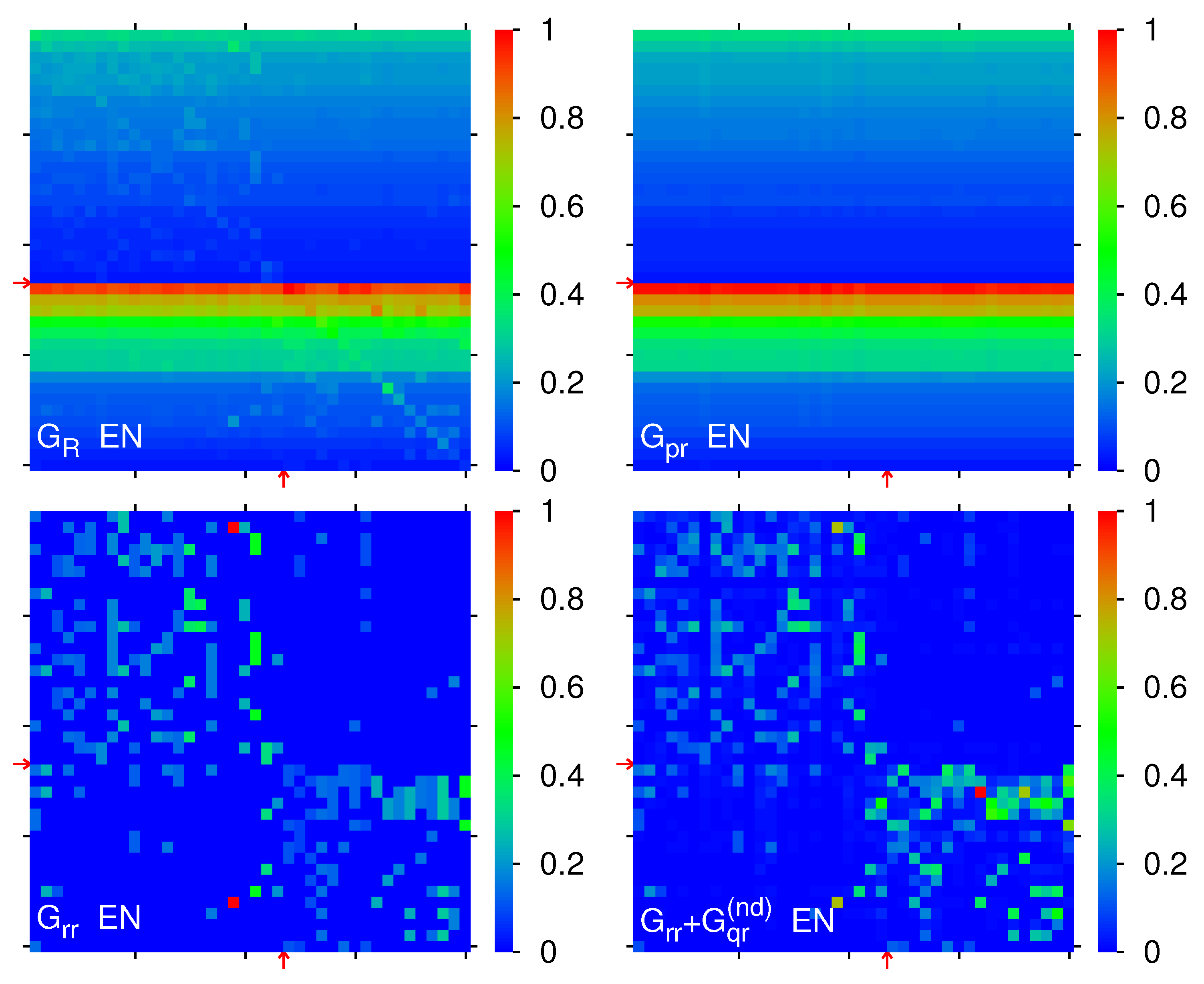
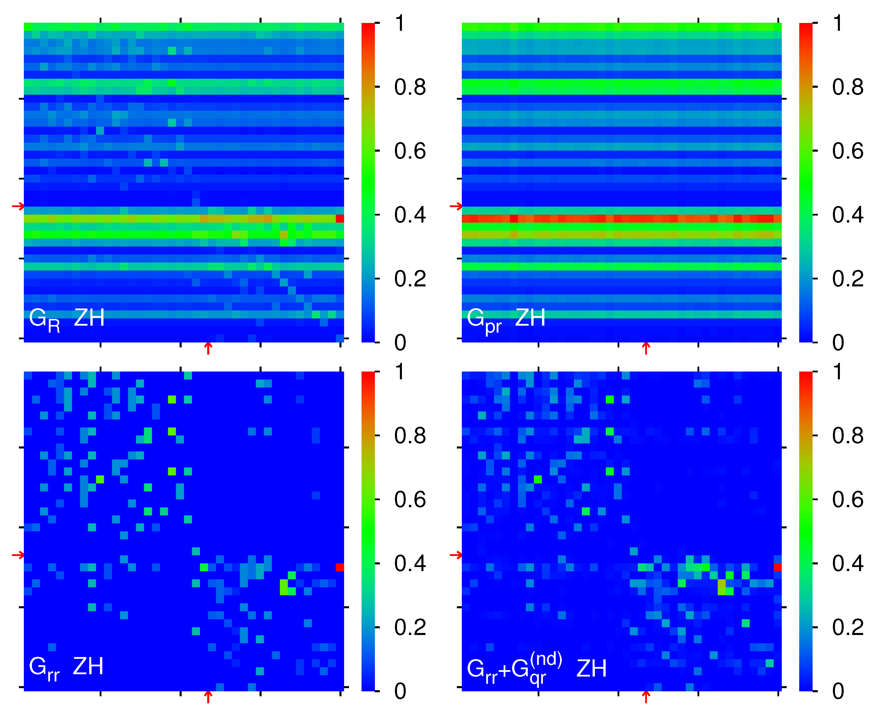
In Figure 3, we show color density plots for G R , G pr , G rr and G rr + G qr ( nd ) for the edition EN with numerical weights being W R = 1 , W rr = 0.0144 , W pr = 0.9661 , W qr = 0.0194 ( W rr + W qr ( nd ) = 0.0280 ). The color plot of G pr is essentially composed of rows of equal color with matrix elements G pr ( i , j ) P r ( i ) for all columns j. Here the sequence of row colors illustrates the separate PageRange order in the two blocks. The row with red color corresponds to the top PageRank node “Catholic Church” with K = 1 , K g = 24 , first row in the religion block, and the rows below at K g = 25 , , 29 with orange or (strong) green color correspond to K = 2 , , 6 . The color plot of G R is similar in appearance, due to the strong weight of G pr , but with additional peaks at isolated positions with largest elements of G rr or G qr (including some quite strong diagonal elements of G qr , especially in the religion block).
For G rr + G qr ( nd ) the strongest matrix elements G rr ( i , j ) + G qr ( nd ) ( i , j ) for each block A, B, C and D (for links i j ) correspond to: 0.0126 (Education ← Oligarchy, A); 0.0021 (Economy ← Chinese folk religion, B); 0.0125 (Shia Islam ← Oligarchy, C); 0.0172 (Islam ← Sunni Islam, D). The last value appears as a sum of a direct link and also a stronger indirect link from Sunni Islam to Islam while the two links from Oligarchy to Education or Shia Islam result from direct links also clearly visible in G rr .
We also observe that the two diagonal blocks A and D seem rather decoupled with significantly smaller links in the off-diagonal blocks B and C which is also confirmed by the sum ratios R ( C , A ) = 0.2778 , R ( B , D ) = 0.0996 , R ( D , A ) = 0.8998 . The value of R ( D , A ) is above to the ratio of areas ( 17 / 23 ) 2 0.55 showing that the transitions inside the religion block D are more intense comparing to the society concepts block A, this difference is also related to the particularly strong maximal element in the D block (see above). The decoupling between the two blocks, which is also be confirmed for the other 7 Wikipedia editions discussed below, seems to be surprising in view of the important historical role played by religions in society formation. However, on the other side there is a well known statement from the Bible: Render unto Caesar the things that are Caesar’s, and unto God the things that are God’s (Bible Matthew 22:21 [35]) that may be partially at the origin of this result. Also in certain countries, e.g. France, the separation between the state and religions is fixed by law.
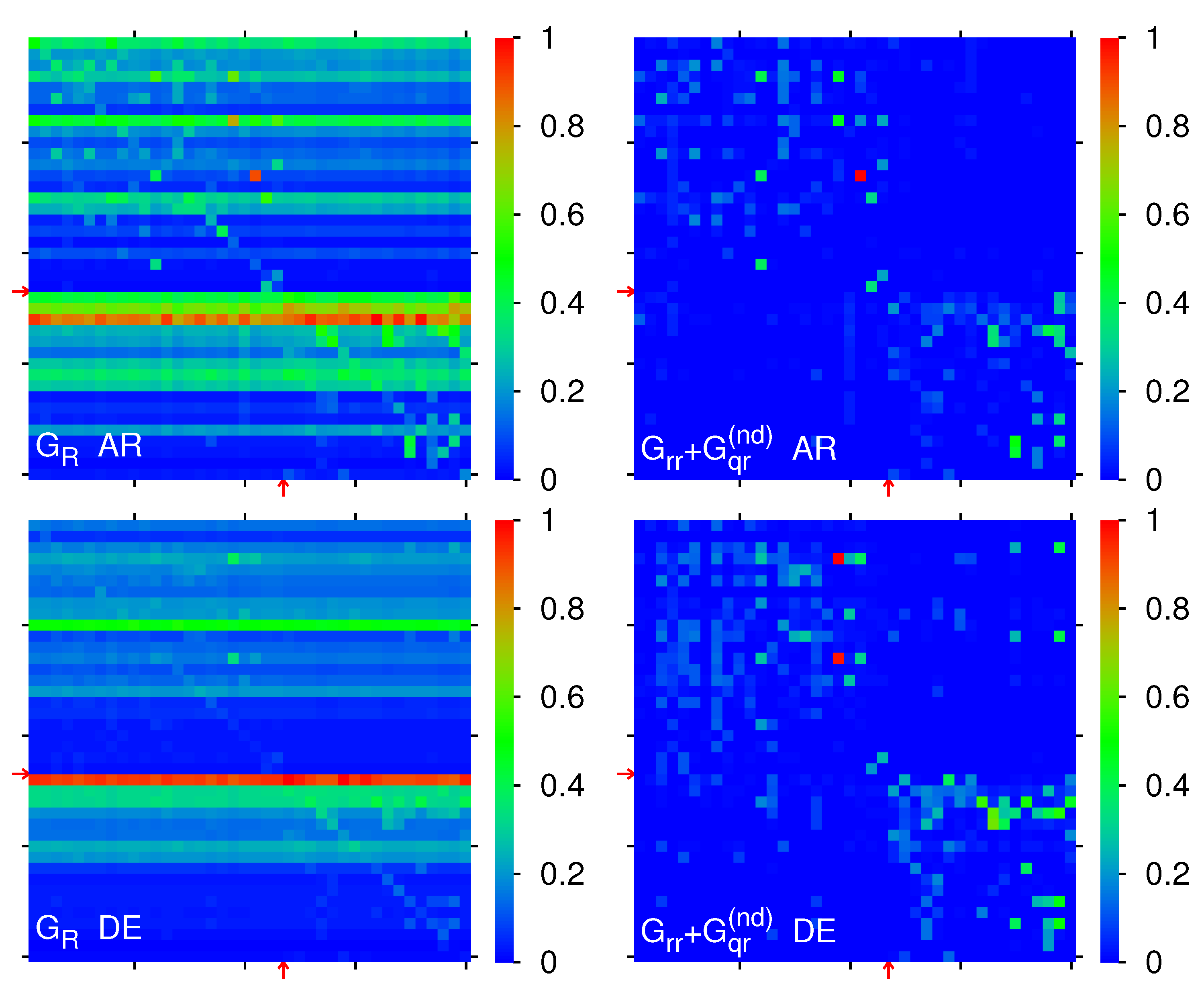
Figure 4 shows the matrices G R and G rr + G qr ( nd ) for the two editions A R and D E . For AR we have the weights W pr = 0.9153 , W rr = 0.0452 , W qr = 0.03936 with higher weights of G rr and G qr as compared to EN. For AR the strongest matrix elements of G rr + G qr ( nd ) per block correspond to: 0.1067 (Monarchy ← Autocracy, A); 0.0063 (Law ← Catholic Church, B); 0.0132 (Islam ← Law, C); 0.0524 (Taoism ← Confucianism, D). The first element of this list is related to the fact that several islamic countries are monarchies. The sum ratios are R ( C , A ) = 0.1311 , R ( B , D ) = 0.1053 , R ( D , A ) = 0.7031 . Here in the panel of G R one sees a strong red row at K g = 26 for the top PageRank node Islam.
In a similar way, we obtain for DE W pr = 0.9582 , W rr = 0.04200 , W qr = 0.0217 and here the strongest matrix elements of G rr + G qr ( nd ) per block correspond to: 0.0327 (Democracy ← Oligarchy, A); 0.0137 (Communism ← Chinese folk religion, B); 0.0058 (Islam ← Republic, C); 0.0209 (Hinduism ← Jainism, D). The sum ratios are R ( C , A ) = 0.1364 , R ( B , D ) = 0.1847 , R ( D , A ) = 0.8417 . As for EN there is a red row for G R at K g = 24 for Catholic Church.
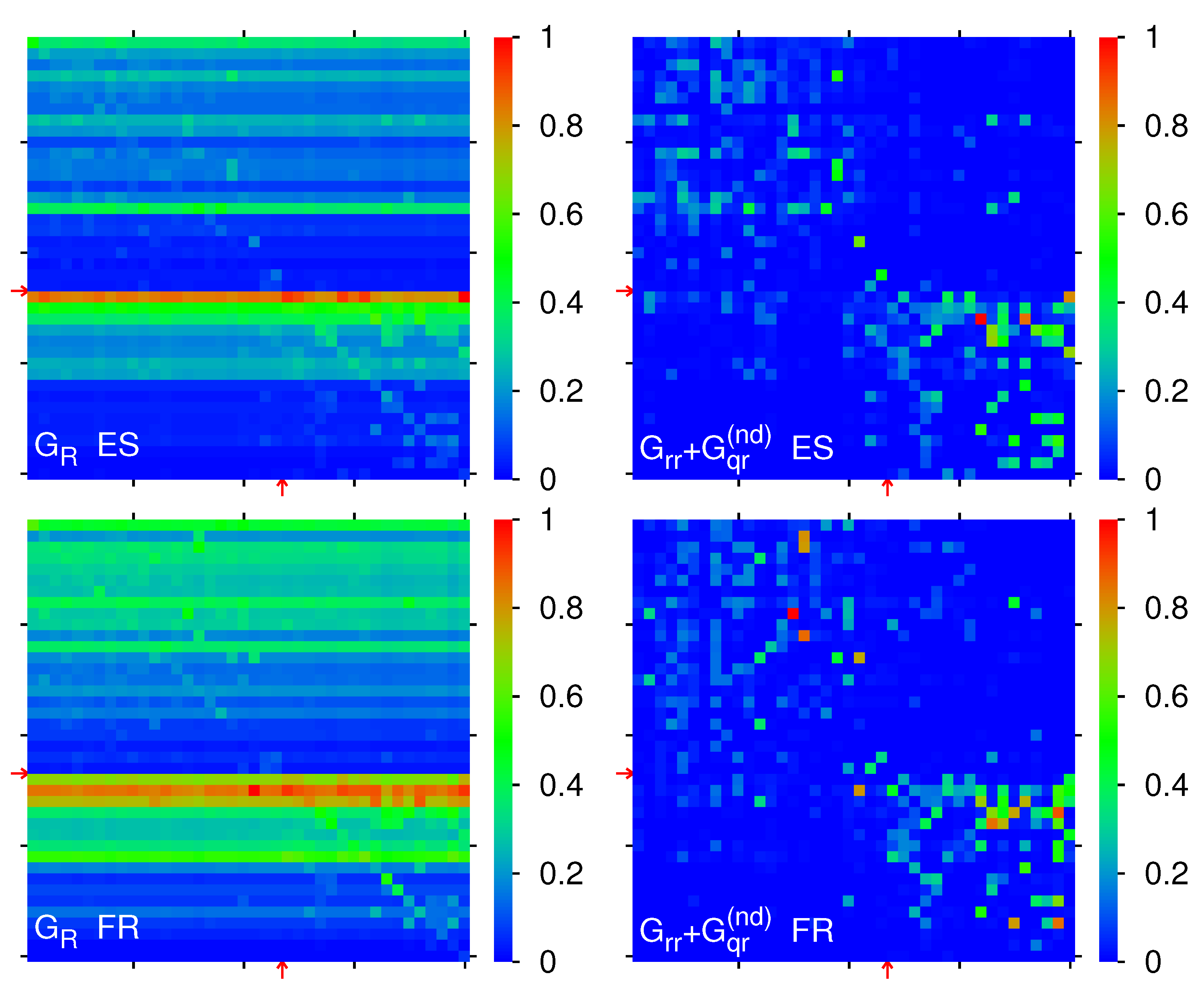
For the ES edition (top panels of Figure 5) we find W pr = 0.9372 , W rr = 0.0269 , W qr = 0.0358 and the strongest matrix elements of G rr + G qr ( nd ) per block correspond to: 0.0222 (Oligarchy ← Autocracy, A); 0.0117 (Society ← Confucianism, B); 0.0082 (Buddhism ← Materialism, C); 0.0346 (Islam ← Sunni Islam, D). Here we have in the D block a second very strong matrix element with value 0.0296 (Islam ← Shia Islam). The sum ratios are given by R ( C , A ) = 0.2170 , R ( B , D ) = 0.1403 , R ( D , A ) = 1.0227 . As for EN and DE there is a red row for G R at K g = 24 for Catholic Church.
For FR (bottom panels of Figure 5) we have W pr = 0.9572 , W rr = 0.0197 , W qr = 0.0229 and the strongest matrix elements of G rr + G qr ( nd ) per block correspond to: 0.0222 (Culture ← Society, A); 0.0101 (Politics ← Confucianism, B); 0.0178 (Christianity ← Autocracy, C); 0.0198 (Buddhism ← Chinese folk religion, D) with additional strong matrix elements 0.0191 (Capitalism ← Economy, A), 0.0179 (Education ← Economy, A), 0.0176 (Communism ← Economy, A), 0.0189 (Taoism ← Chinese folk religion, B) and 0.0170 (Monarchy ← Autocracy, A). We attribute the last link and the top C link from Autocracy to Christianity to the baptême de Clovis when the king of France Clovis I accepted the Christian religion around the year 500. The sum ratios are R ( C , A ) = 0.1894 , R ( B , D ) = 0.1395 , R ( D , A ) = 1.1519 . There is a red row for G R at K g = 25 , K = 1 for Christianity along with strong orange rows at K g = 26 , K = 2 (Islam) and K g = 24 , K = 3 (Catholic Church).
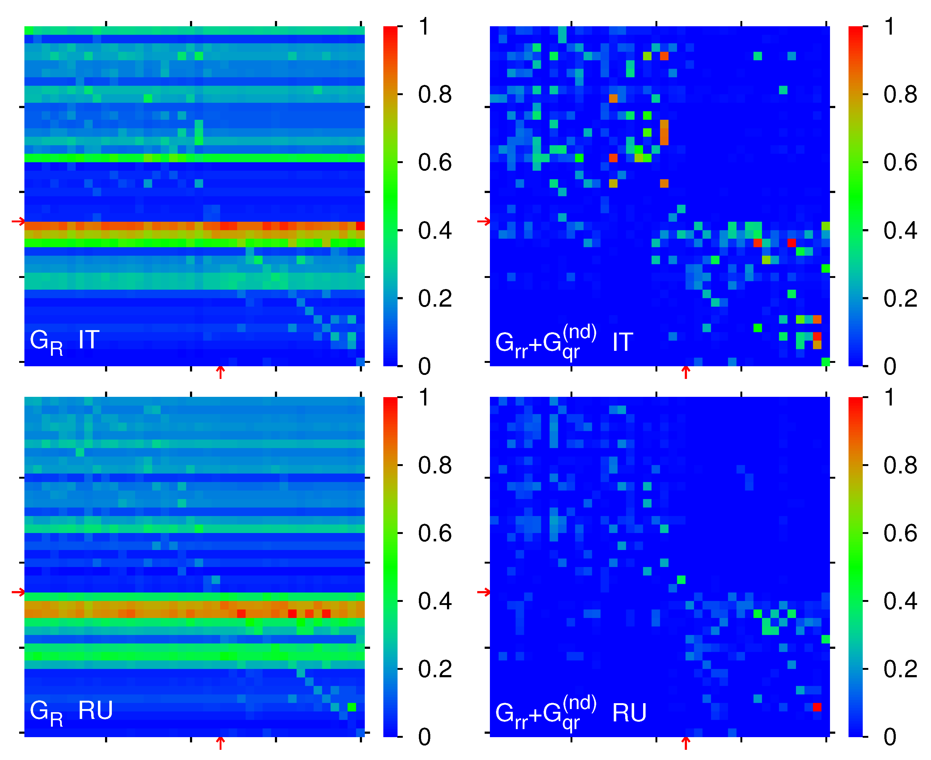
For the IT edition (top panels of Figure 6) the matrix weights are W pr = 0.9393 , W rr = 0.0297 , W qr = 0.0308 and the strongest matrix elements of G rr + G qr ( nd ) per block correspond to: 0.0298 (Economy ← Society, A); 0.0108 (Democracy ← Sunni Islam, B); 0.0095 (Christianity ← Idealism, C); 0.0326 (Islam ← Shia Islam, D). Furthermore there are significant numbers of additional strong matrix elements in the D-block: 0.0313 (Taoism ← Chinese folk religion); 0.0307 (Islam ← Sunni Islam); 0.0285 (Confucianism ← Chinese folk religion); 0.0260 (Shinto ← Chinese folk religion) and also in the A-block: 0.0292 (Democracy ← Autocracy); 0.0280 (Fascism ← Autocracy); 0.0278 (Monarchy ← Autocracy); 0.0273 (Oligarchy ← Autocracy); 0.0272 (Culture ← Society); 0.0266 (Republic ← Autocracy), the latter probably being related to Italian history. The sum ratios are given by R ( C , A ) = 0.1372 , R ( B , D ) = 0.1159 , R ( D , A ) = 0.6477 and there are two strongs rows for G R being red ( K g = 24 , K = 1 , Catholic Church) and orange ( K g = 25 , K = 2 , Christianity).
For RU (bottom panels of Figure 6) we have W pr = 0.9515 , W rr = 0.0217 , W qr = 0.0267 and the strongest matrix elements of G rr + G qr ( nd ) per block correspond to: 0.0223 (Materialism ← Idealism, A); 0.0043 (Capitalism ← Protestantism, B); 0.0066 (Buddhism ← Civilization, C); 0.0569 (Taoism ← Chinese folk religion, D). Here we have the sum ratios R ( C , A ) = 0.1519 , R ( B , D ) = 0.0928 , R ( D , A ) = 0.7268 and in the G R panel we see two orange-red rows at K g = 26 , K = 1 (Islam) and, with slightly smaller values, at K g = 25 , K = 2 (Christianity).
Finally, in Figure 7 we show the matrices for G R , G pr , G rr and G rr + G qr ( nd ) of the ZH edition. Here the weights are: W pr = 0.9233 , W rr = 0.0333 , W qr = 0.0432 ( W rr + W qr ( nd ) = 0.0658 ). For ZH the strongest matrix elements of G rr + G qr ( nd ) per block correspond to: 0.0341 (Fascism ← Nazism, A); 0.0097 (Education ← Judaism, B); 0.0219 (Christianity ← Idealism, C); 0.0653 (Christianity ← Oriental Orthodox Churches, D) and the block-sum ratios are R ( C , A ) = 0.2639 , R ( B , D ) = 0.1319 , R ( D , A ) = 0.8458 . In the panel of G pr we see a strong red row at K g = 25 , K = 1 (Christianity), which appears less pronounced (between orange and strong green) in the other panel of G R but mainly because the very strong maximal direct matrix element in the D-block of G rr (and of G rr + G qr ( nd ) corresponding to the link Christianity ← Oriental Orthodox Churches) shifts the maximum value in the color plot defining the red color which reduces the color scale of other matrix elements. We note that the structure of the matrix G rr + G qr ( nd ) follows for ZH mainly G rr for the strongest transitions.
The results of this subsection show that for the matrices G rr + G qr ( nd ) of all 8 editions there are indeed multiple significant transitions inside both blocks of society concepts and of religions. However, the transitions between these two blocks are, roughly by a factor 5-10, smaller if we compare the sums of matrix elements of the off-diagonal block to the sums over the diagonal blocks. The ratio of transition strengths of the two diagonal blocks is typically R ( D , B ) somewhat larger than the ratio ( 17 / 23 ) 2 0.55 of block areas D , B . This shows that transitions between religions are on average a bit stronger than those between society concepts.

4.3. Network Structure Inside Social Concepts and Religions

In this section, we present effective network diagrams for friends and followers based on the information contained in the matrix G rr + G qr ( nd ) or more precisely in its two diagonal blocks A for society concepts and D for religions. Since, according to the results of the last subsection, these two blocks are rather well decoupled with only weak links between them, we will present separate network diagrams for each block. Network diagrams of (nearly) the same style, were for example used in [22] (for groups of political leaders in the Wikipedia network), [25] (for banks and countries in the Wikipedia network), and [27] (for a specific fibrosis related protein group in the MetaCore network of proteins).
However, for convenience, we present here the construction method of these network diagrams. Assume we have a small matrix g with elements g ( i , j ) being either a reduced Google matrix or one of its components (e.g. G R , G rr , G qr or G rr + G qr ( nd ) ) or a certain sub-block of such a matrix (e.g. society or religion sub-blocks A or D of G rr + G qr ( nd ) shown in the previous section). First, we choose in the list of nodes (associated to this matrix or block) 5 top nodes representing five different subgroups based on some categorization criteria (depending on the set of nodes and the context) and we attribute each other node of this list to exactly one of the 5 subgroups (based on some criteria and the context). In the following, we will use for these subgroups the notation poles as a synomym for “center of interest” which is a typical use of this expression in the French language. For each pole, we also define some presentation color.
To construct the effective friend network (see below for the other case of follower networks), we draw first a main circle (thin gray line) and place the 5 top nodes uniformly on this circle with some label and the corresponding color. Then we select for each top node j (also called level-1 nodes) the four strongest friends i (level-2 nodes) with strongest outgoing links j i , i. e. with largest matrix elements g ( i , j ) in the same column j of this matrix. Each of these strongest friends, if not yet present in the diagram as another level-1 node, is placed on a smaller secondary circle around the top level-1 node associated to him and we draw thick black arrows from the level-1 nodes to their friends. It is possible that a new level-2 node appears as a friend of several initial level-1 nodes. In this case, we try first to place this level-2 node on the circle of the level-1 node with same color (same pole) if possible, i. e. if this level-2 node is indeed a friend of the level-1 node of same color. Only if this is not possible, we place it on the circle of another level-1 node (first level-1 node of different color which has the given level-2 node as friend). If a level-1 node has a friend which is already present in the diagram as another level-1 node, we simply draw a thick black arrow from the former to the latter and do not modify the position of the latter.
The procedure is repeated for all (newly added) level-2 nodes with smaller circles around them on which we place their (up to) four strongest friends (level-3 nodes if newly added) and with the same rule for preferential placement on a circle of a parent node of same color. Now, we draw thin red arrows from the level-2 nodes to their friends. In case if such a friend is already present in the network (as level-1 or level-2 node), his position is not modified and we only draw the thin red arrow from his parent node to him. We also mention that only non-empty circles with at least one node on them are drawn; i. e. if a given node has no newly added friends (i. e. all his friend are already in the diagram), then we will not draw an empty circle around him.
At this stage, we typically stop the procedure for simplicity. Even if we continue this procedure with level-4, level-5 nodes etc. the number of newly added nodes quickly decreases and when there is no newly added node the procedure converges to a stable final diagram. This can happen actually quite early so that their is typically no big difference in diagrams limited to level-3 nodes and those with higher level nodes. In particular, for the diagrams given below, the number of newly added level-3 nodes is typically already quite small (much smaller than the theoretical limit 5 × 4 × 4 = 80 ) also because the available set of nodes is limited from the very beginning, even significantly smaller than the theoretical level-3 limit. In some of the diagrams below there are even no newly added level-3 nodes (if absence of smallest level-3 circles) and we have already convergence to a stable diagram at level-2, i. e. all friends of level-2 nodes are already present in the diagram as former level-1 or level-2 nodes. In case of convergence, the last stage does not add new nodes but it still adds arrows from the most recently added nodes in the previous stage to their friends (which are already present in the network diagram).
The construction of follower network diagrams is essentially the same with two modifications: (i) at each level k we select for each level-k node i (typically only k = 1 , 2 in our case) the four strongest followers j (as possible level- ( k + 1 ) node if not yet present in the diagram) with strongest incoming links i j defined by the largest matrix elements g ( i , j ) in the same row i; (ii) arrows (thick black or thin red) are drawn with inverted directions from followers (level- ( k + 1 ) nodes) to parents (level-k nodes), e.g. there are some arrows from a circle node to its center node while in the friend diagrams we have arrows from the circle center to the outside nodes on the circle (note in case of multiple parent nodes or pre-existing friends or followers, we have typically a significant number of other type of arrows between different circles).
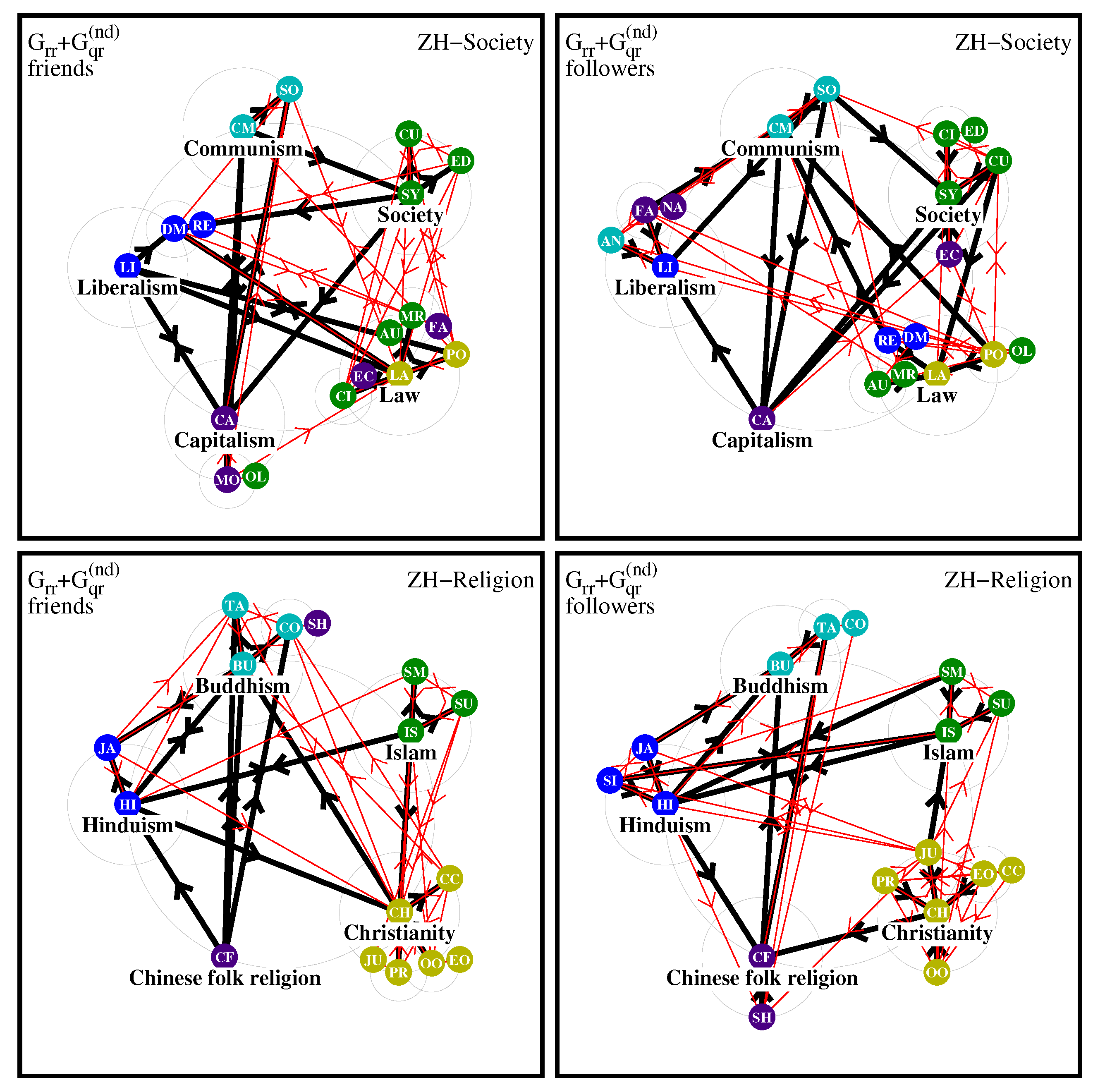
In this work, we present figures for the network diagrams constructed from the two diagonal blocks A for society related nodes and D for religions of the matrix G rr + G qr ( nd ) for the 8 different Wikipedia editions. Since there are two friend and follower diagrams for each case, we have per edition four network diagrams presented in a figure with four panels. The subgroups or poles together with their respective 5 top nodes for both society and religion cases are given in Table 2 (8th column) and this table also contains a two letter code for each node (5 th column) used as a node label in the diagrams.
For society concepts, we choose the 5 top pole nodes Law, Society, Communism, Liberalism and Capitalism with respective node colors being olive, (dark) green, cyan, blue and indigo. We have tried to attribute the members of the poles based on the context and logical proximity to the top node, e.g. Education and Culture are attributed to the 2nd pole of Society; Ecology, Politics belong to the first pole of Law; Socialism and Anarchism are attributed to the 3rd pole for Communism. In certain cases, this attribution is a bit arbitrary and other choices would have been possible. We also tried to assure that each pole has a certain minimum number of members.
For the religion nodes, we choose the 5 top pole religions Christianity, Islam, Buddhism, Hinduism and Chinese folk religion (same colors as for the society top nodes in this order) and with its pole members being related to branches of religions or sub-religions. Here, we have attributed Judaism to the 1st Christianity pole with other members being Catholic Church, Protestantism and both nodes about Orthodox Church.
In the following, we will more precisely call this poles also “initial poles” in order to distinguish them from “natural poles” which may emerge naturally by certain clusters in a network diagram. Quite often natural poles and initial poles are very similar but in certain cases natural poles are composed of nodes from several initial poles.
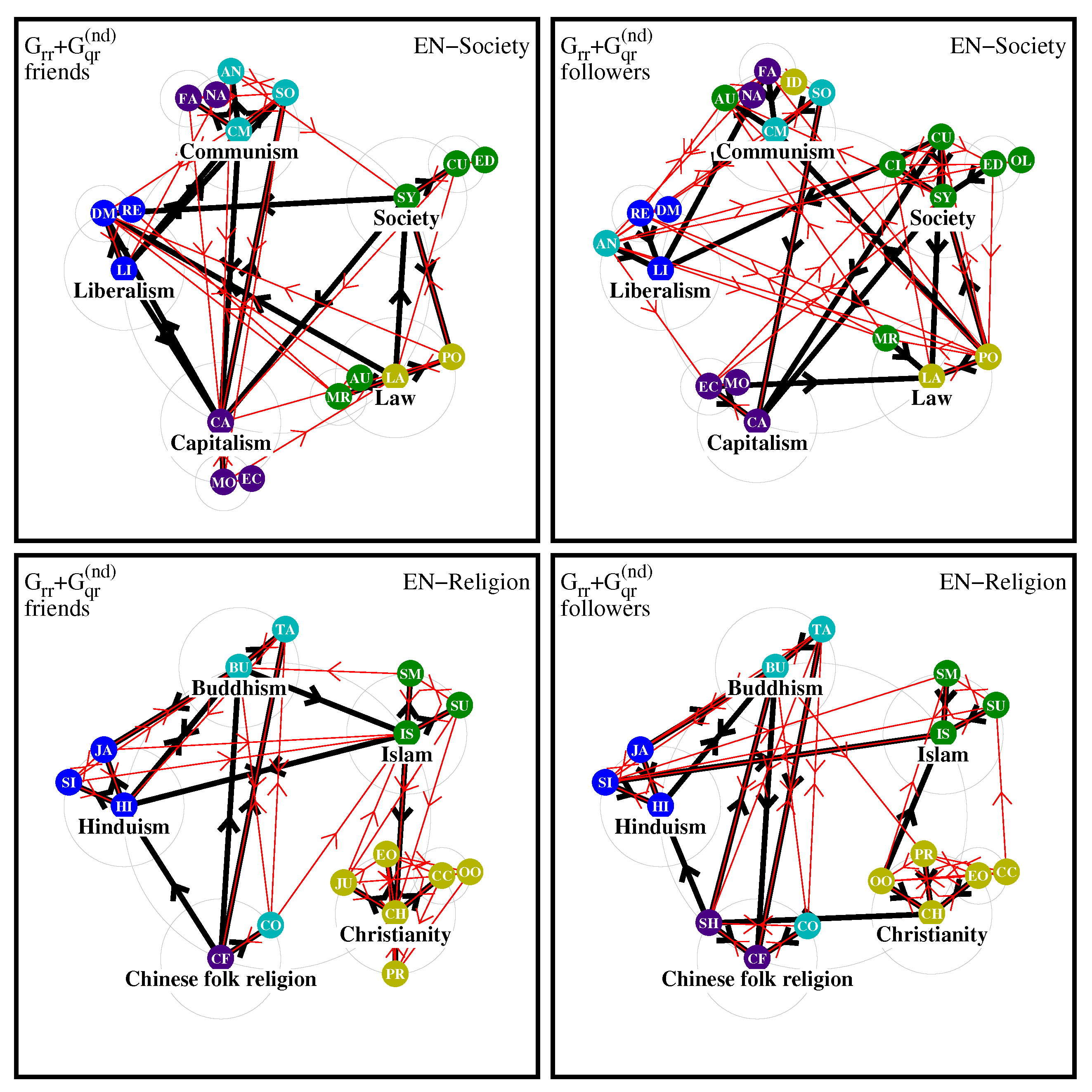
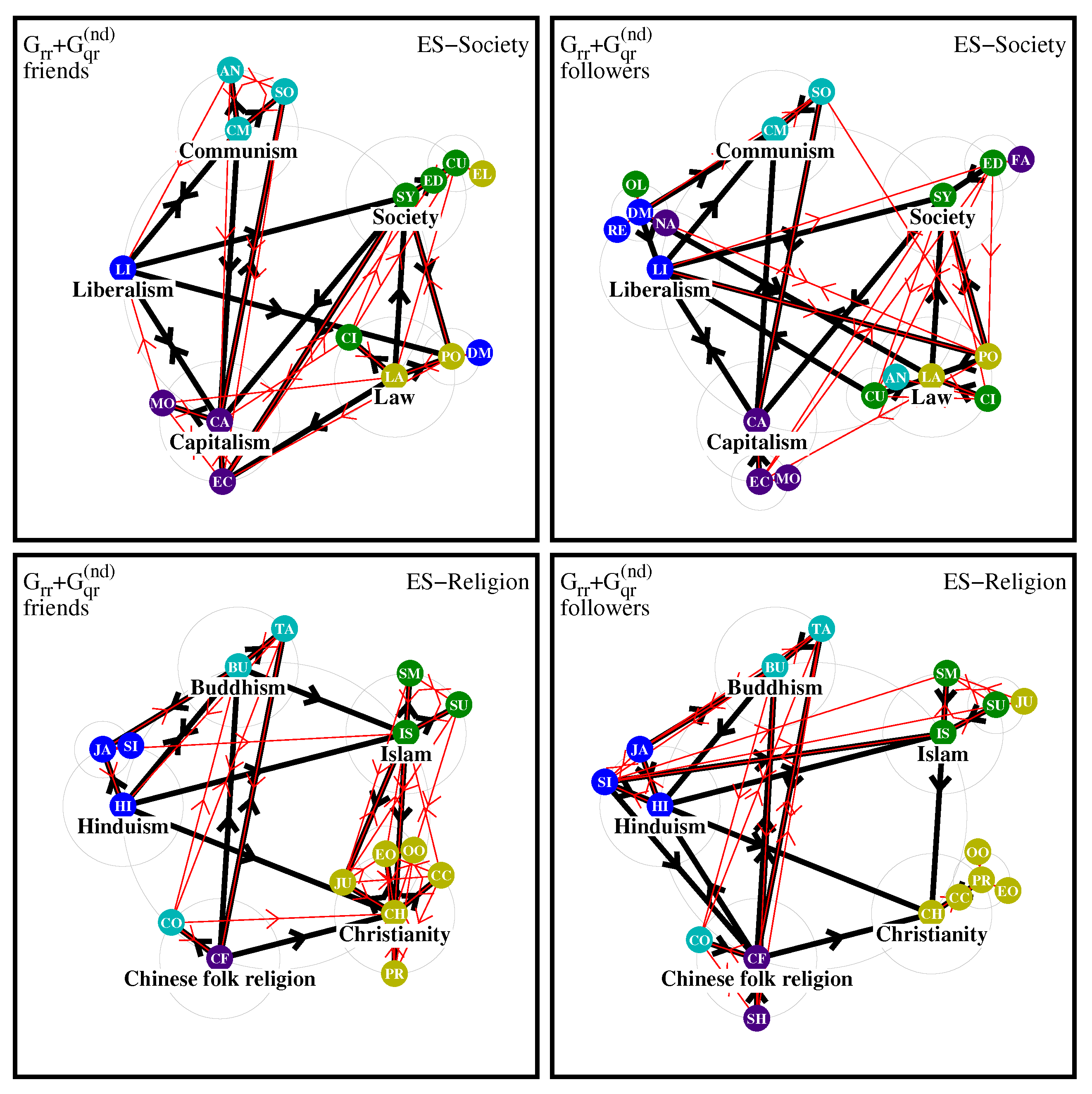
Specifically, for the EN edition, whose network diagrams are shown in Figure 8, we can identify in the friend society diagram the formation of 5 natural poles (which may slightly deviate from the initial poles) with main members being 1T) Law, Politics, Monarchy, Autocracy (2 initial poles); 2T) Society, Culture, Education (1 initial pole); 3T) Communism, Socialism, Anarchism, Nazism, Fascism (2 initial poles); 4T) Liberalism, Democracy, Republic (1 initial pole) and 5T) Capitalism, Money, Economy (1 initial pole). Thus the natural pole Communism has the largest number of diagram members even if it is composed of nodes belonging to two different initial poles.
The diagram of followers has the natural poles 1T) Law, Politics, Monarchy (2 initial poles); 2T) Society, Culture, Education, Civilization, Oligarchy (1 initial pol); 3T) Communism, Socialism, Fascism, Nazism, Autocracy, Idealism (5 initial poles); 4T) Liberalism, Democracy, Republic, Anarchism (2 initial pol); 5T) Capitalism, Money, Economy (1 initial pol). Thus again the strongest natural pole is formed around Communism.
For the diagram of religion friends we have from Figure 8 the natural pole members: 1T) Christianity, Catholic Church, Eastern Orthodox Church, Judaism, Protestantism, Oriental Orthodox Churches (1 initial pol); 2T) Islam, Sunni Islam, Shia Islam (1 initial pol); 3T) Buddhism, Taoism (1 initial pol); 4T) Hinduism, Jainism, Sikhism (1 initial pol); 5T) Chinese folk religion, Confucianism (2 initial poles). The strongest pole is Christianity, however, it is somehow isolated having strong links only from Islam while the poles of Islam, Buddhism, Hinduism, Chinese folk religion have more active interconnections.
For the diagram of religion followers we find: 1T) Christianity, Eastern Orthodox Church, Protestantism, Oriental Orthodox Churches, Catholic Church (1 initial pole); 2T) Islam, Sunni Islam, Shia Islam (1 initial pole); 3T) Buddhism, Taoism (1 initial pole); 4T) Hinduism, Jainism, Sikhism (1 initial pole); 5T) Chinese folk religion, Confucianism, Shinto (2 initial poles). Here the strongest pole is again Christianity, and now it is less isolated with connections to Islam and Chinese folk religion. At the same time we see here more intense links between religions from Asia (3T, 4T, 5T) forming a strongly interconnected religion group.
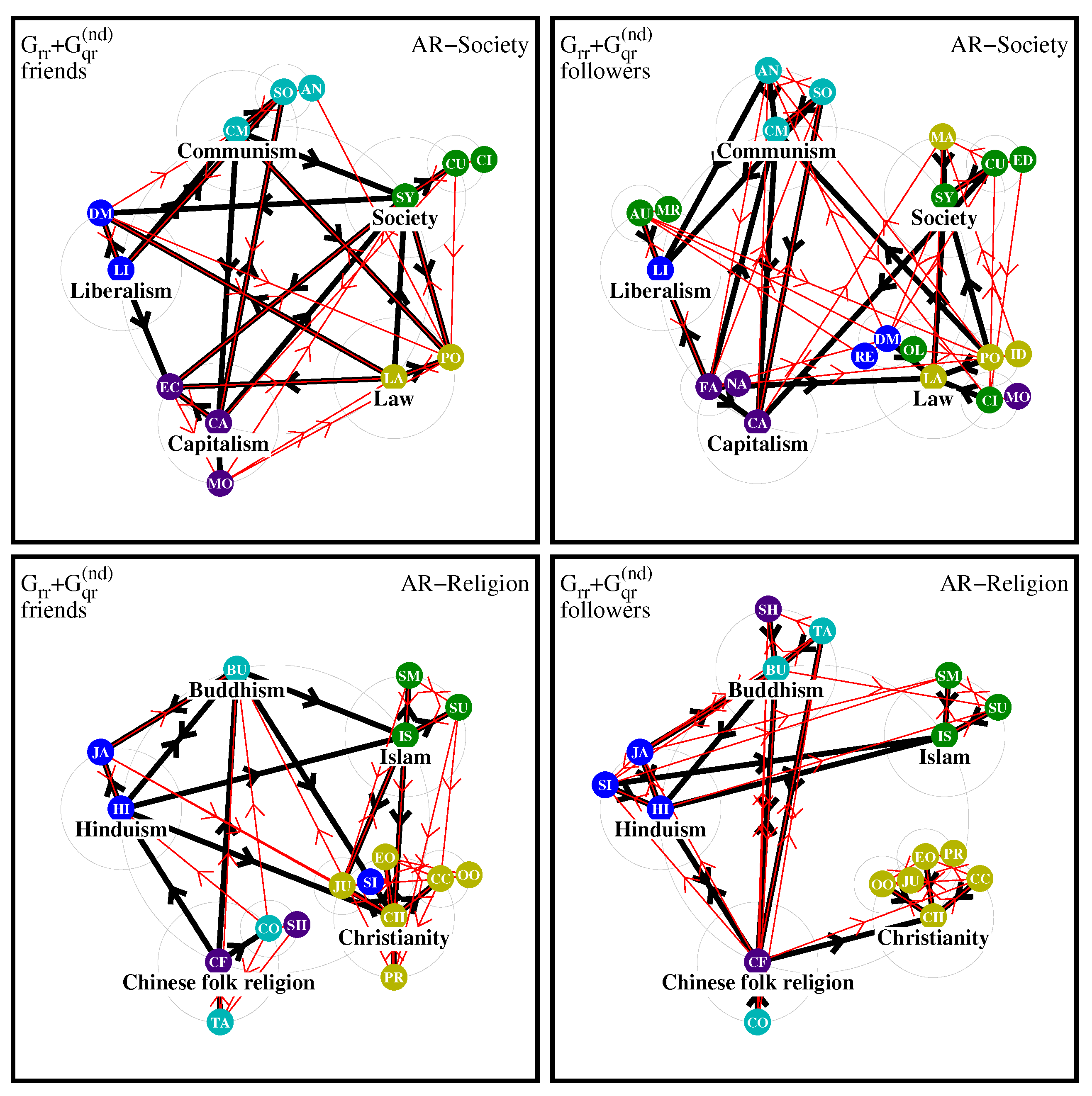
The diagram of friends for society concepts of AR, whose network diagrams are shown Figure 9, has a reduced number of nodes as compared to EN in Figure 8, but the poles are more interconnected by strong links. Interestingly, the Communism pole does not include Fascism, Nazism in contrast to the EN edition. For the diagram of society followers the natural pole with largest number of nodes is Law with 7 members and 4 initial poles, The Communism pole includes only Socialism and Anarchism in contrast to EN where the (natural) pole of Capitalism also includes Fascism and Nazism.
For the AR diagram of friends for religions in Figure 9, we see that the Christianity pole contains a larger number of members as in the EN case but there are more links between poles and the Christianity pole is not as isolated as it is for EN. However, for the diagram of followers the Christianity pole remains more isolated compared to the EN, also there are no strong black links between Christianity and Islam.
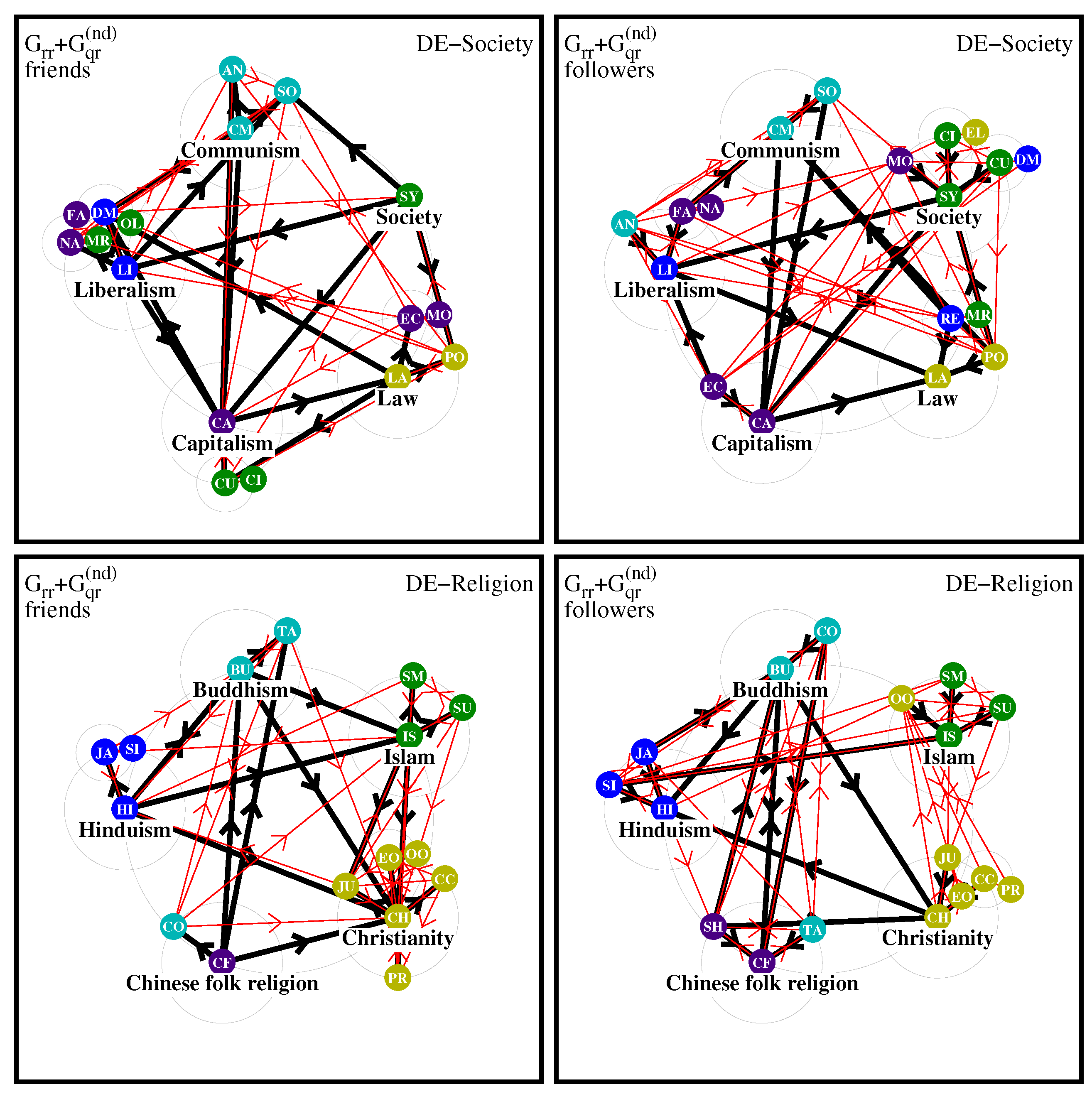
For the DE edition the diagrams are presented in Figure 10. For the diagram of friends for society concepts the strongest natural pole is Liberalism with Democracy, Fascism, Nazism, Monarchy and Oligarchy (3 initial poles) while for EN Fascism and Nazism are included in the Communism pole; also for DE the poles are more densely interconnected as compared to EN. For the diagram of followers, we again see a significant difference with EN, thus Fascism and Nazism are included in Liberalism pole while they are in the Communism pole for EN.
For the DE religion diagrams we have denser interconnections between the 5 poles as compared to EN. In the case of followers there are no strong links between Islam and Christianity but there are many (level-2) red links between their respective pole members.
For the ES edition the network diagrams are given in Figure 11. Its society friend diagram is similar to EN but there are less nodes in the Liberalism pole (i. e. the direct friends of Liberalism are the other four level-1 top nodes), also Fascism and Nazism are absent. For the case of followers there are less pole members for Society, Communism but more for Law and Liberalism; Nazism is attributed to the Liberalism pole, Nazism is absent which is different from the EN case.
For the religion diagrams of ES in Figure 11 the case of friends is similar to those of the EN edition but there are less links between the Islam and Christianity poles.
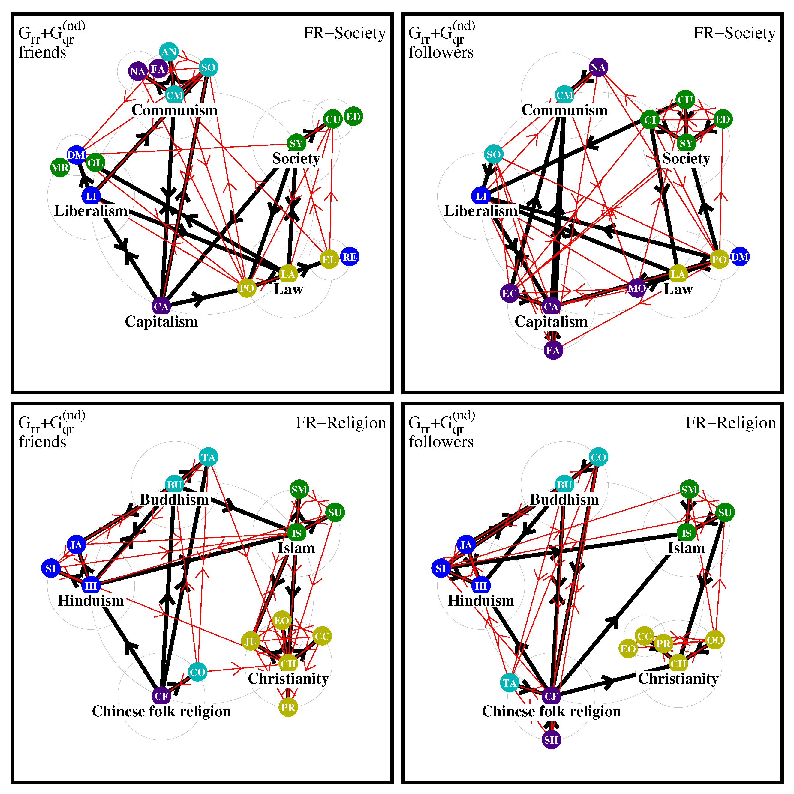
For the FR edition the network diagrams are shown in Figure 12. Here the society friend diagram is similar to the case of EN but with less links between the Society and Liberalism poles; as for EN the nodes Nazism and Fascism belong to the Communism natural pole. For the case of followers the Communism pole has only one node Nazism (from another initial pole) while for EN this pole contains 6 members including Fascism and Nazism. The religion diagrams of FR are quite similar with those of EN.
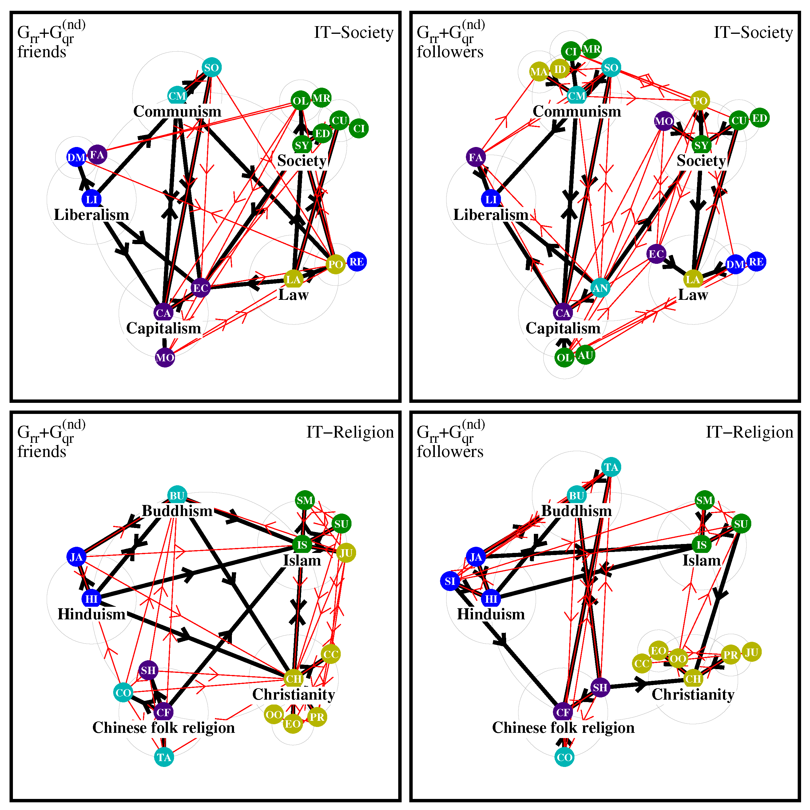
The network diagrams for the IT edition are presented in Figure 13. For the society friend diagram the largest pole is Society including Culture, Education, Civilization, Oligarchy and Monarchy (all nodes from the same initial pole); the Liberalism pole includes Democracy and Fascism while Communism has only Socialism that makes the last two poles rather different from the EN edition; the Capitalism pole is the same as for EN case; the Law pole contains only Politics and Republic. For the society follower network of IT the highest number of members is in the pole of Communism including Socialism, Materialism, Idealism, Civilization and Monarchy (3 initial poles). In both society friend and follower diagrams, thoe node Fascism is attributed to Liberalism and while Nazism is absent which constitutes a drastic difference with the EN case.
In the religion friend diagram of IT the node Christianity has the highest number of nodes and it is strongly linked with Islam, Buddhism and Hinduism in contrast to EN where this pole is more isolated. The diagram of followers is similar to those of the EN edition and Christianity remains the strongest pole.
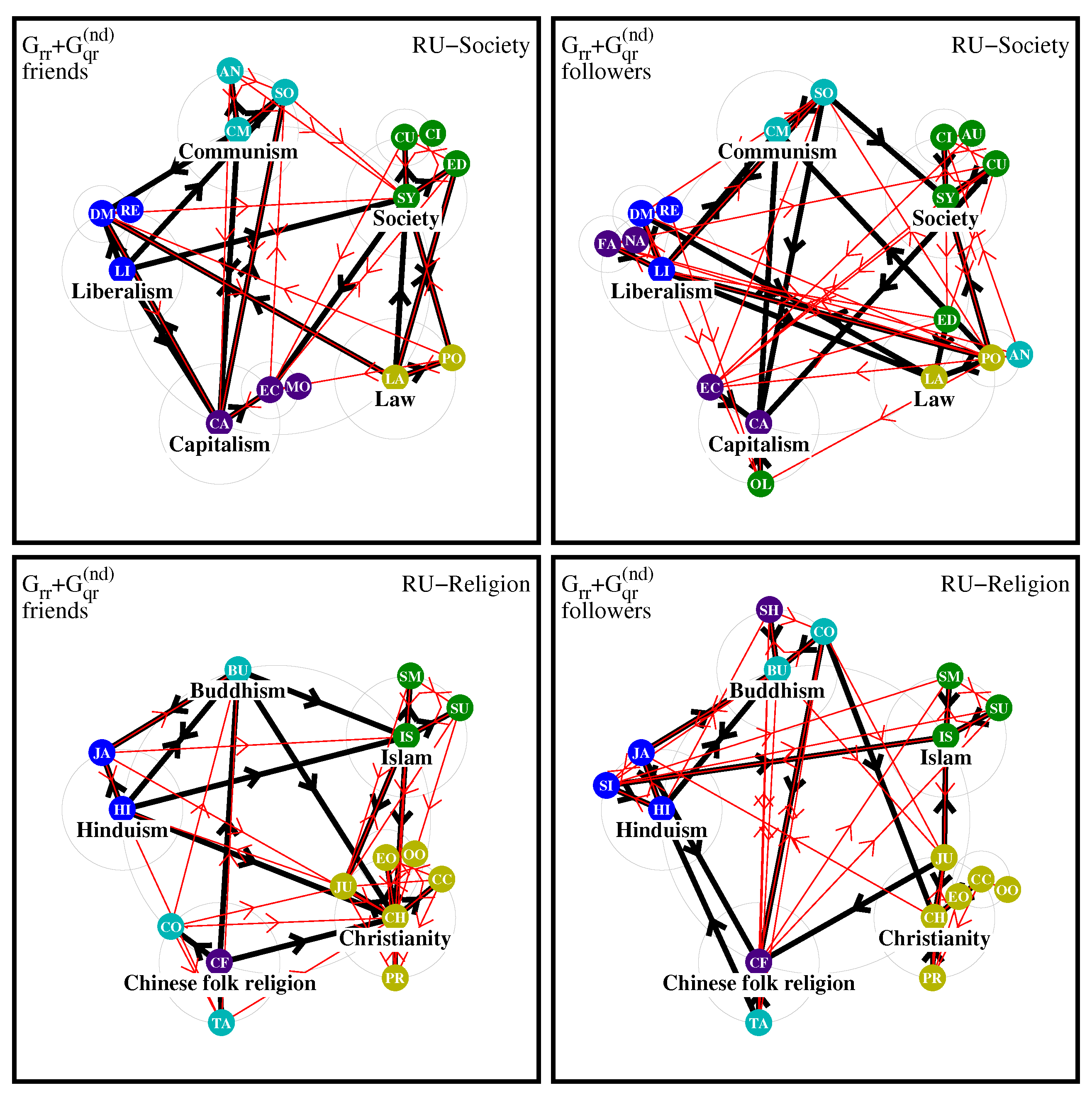
In Figure 14 we show the network diagrams for the RU edition. Here the society friend diagram is similar to EN but without Fascism, Nazism in the diagram, also poles Law and Society have a bit less of included nodes. In the diagram of followers Fascism and Nazism are included in the Liberalism pole in contrast to the EN edition where these 2 nodes are included in Communism pole.
For the religion friend diagram Christianity has the largest number of nodes including Judaism linked also from Islam and this pole is less isolates as in the EN edition. For the diagram of religion followers Christianity is still the largest pole with 6 nodes including Judaism pointing to Islam but in other aspects this diagram is similar to the EN edition.
Finally, for the edition ZH the diagrams are presented in Figure 15. In the society friend diagram the strongest pole is Law including Politics, Civilization, Autocracy, Monarchy, Economy and surprisingly Fascism. We note that for ZH the node Law has the unusual local Rank value K = 3 for a society node which are normally well behind the religion nodes in PageRank order. The Communism pole includes only Socialism being well linked to the Society pole, in contrast to the EN case; Liberalism and Capitalism poles are similar to EN. In the society followers diagram the strongest pole is again Law with 6 nodes and 3 initial poles; Fascism and Nazism are included in the Liberalism pole.
For the religion friend diagram of ZH the strongest pole is Christianity with 6 nodes being well connected to other poles, in contrast to the EN case; at the same time the interlinks between Asian religion poles Buddhism, Hinduism, Chinese folk religion are denser as compared to EN. In the religion follower diagram the strongest pole is also Christianity with 6 nodes, the diagram structure is similar to EN with a larger number of links between Islam and Hinduism poles.

4.4. Proximity and Differences of Cultures

Let us summarize the most important differences and similarities between the 8 cultures represented by the 8 language Wikipedia editions obtained in the last subsection by analyzing the different network diagrams.
First for the society diagrams the English and French cultures attribute the two nodes Fascism and Nazism to the Communism pole while they are attributed to the Capitalism pole by the Arabic culture and to the Liberalism pole by the German, Spanish (partially), Italian (partially), Russian (for followers) and Chinese (for followers) cultures.
Concerning the religion diagrams, the Christianity pole seems to be rather isolated in the English culture with other links only from the Islam pole (in the friend diagram). On the other hand, for the other cultures the Christianity pole is well connected not only with the Islam pole but also with the other poles of Hinduism, Buddhism and Chinese folk religion. For a majority of cultures the three poles of the above Asian religions have a higher density of links between them as compared to the Islam and Christianity poles.
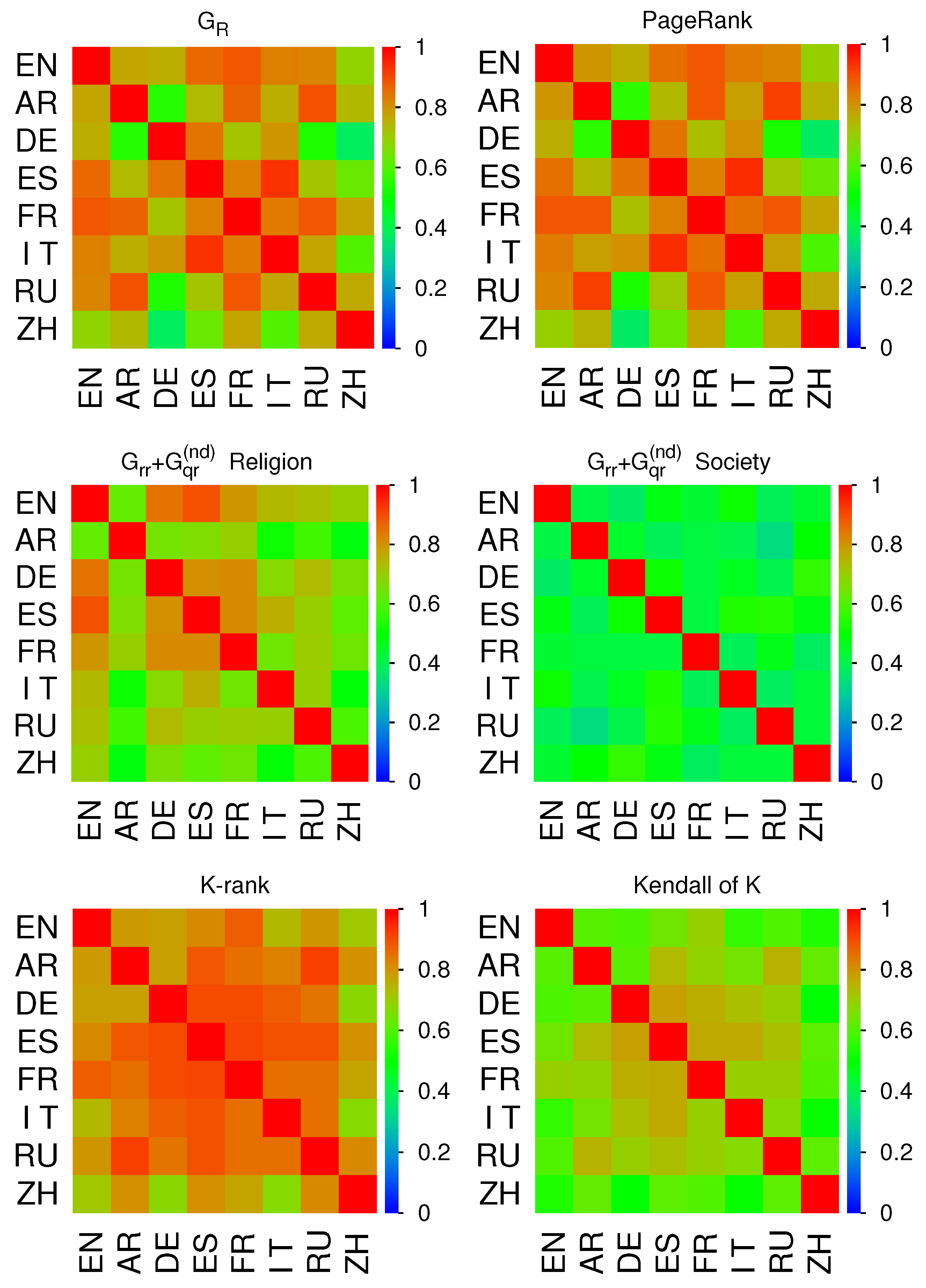
To determine quantitatively the proximity of the 8 cultures, we compute the correlators for certain key quantities shown in Figure 16. The 6 panels of Figure 16 provide 8 × 8 -matrix density plots for different inter edition correlators with 5 panels for the Pearson correlator of 5 quantities being the matrix G R , the (group local) PageRank vector P r , the religion and society sub-blocks for G rr + G qr ( nd ) and the local PageRank index K and one additional panel for the Kendall correlator of K. The precise definitions of these correlator quantities with some additional technical details are given in SubSection 3.4 and we note that for such correlator quantities the minimal mathematical possible value is 1 , for the case of two data sets with strong anti-correlations, while values close to 0 indicate weak or absent correlations and values close to + 1 correspond to strong correlations.
First, we observe that generally all 8 Wikipedia edition seem to be rather well correlated with a big majority of correlator values being above 0.5 and only a few values close to 0.33. The two correlators associated to G R and P r (top row of Figure 16) are very close which is plausible due to the typical strong numerical weight of G pr in G R and the fact that the columns of G pr are close to P r . Here the correlations of DE between AR, RU and ZH seem minimal (still with values 0.5 ) and also ZH seems to be less correlated to the other editions (with some fluctuations). The other inter edition correlations are typically quite strong 0.8 with the largest values 0.93 - 0.94 for the correlation between ES and IT.
More specifically, for the G R -correlator and EN the closest other editions are FR (0.882) and ES (0.858); for AR the largest values are with RU (0.896) and FR (0.867) which appears to be plausible due to the, at least partial, importance of Islam in these three cultures. For DE the two closest cultures are ES (0.845) and IT (0.803); for ES they are IT (0.933) and EN 0.858); for FR they are RU (0.885) EN (0.882); for IT they are ES (0.933) and FR (0.842); for RU they are AR (0.896) and FR(0.885) and finally for ZH they are FR (0.774) and RU (0.767). For the very similar P r -correlator this list of closest two editions is identical with only slightly different correlator values.
Concerning the religion block of G rr + G qr ( nd ) (center left panel of Figure 16), we see that AR and ZH have globally the weakest correlations to the other cultures, with values 0.5 , which seems natural due to the importance of their specific religions. On the other hand here, we have a block of four strongly correlated editions EN, DE, ES, FR between them, with values 0.8 , while IT and RU have typical “intermediate” correlations 0.7 .
More explicitly, for this case the closest cultures of EN are ES (0.892) and DE (0.844); for AR they are FR (0.699) and ES (0.662) with relatively low values; for DE they are EN (0.844), FR (0.814) and ES (0.806); for ES they are EN (0.892), FR (0.814) and DE (0.806); for FR they are DE (0.814), ES (0.814) and EN (0.801); for IT they are ES (0.76) and EN (0.746); for RU they are DE (0.737) and EN (0.73) and finally the strongest correlator of ZH is to EN (0.694).
The society block of G rr + G qr ( nd ) (center right panel of Figure 16) shows the “weakest” general correlations of all correlator quantities with (off-diagonal) values being typically 0.5 with the strongest off-diagonal element being 0.565 between DE and ZH which is due to two strong matrix elements in G rr + G qr ( nd ) due to the links from Oligarchy to Democracy and Monarchy for both editions. Here the AR-RU correlator represents the minimal correlator value 0.332 for all editions and all correlator quantities.
The Pearson and Kendall correlator of the PageRank index K (bottom row of Figure 16) appear to have roughly a similar relative structure as the Pearson correlators of G R and P r (top row of Figure 16). However, here the overall values are significantly stronger (lower) for the Pearson (Kendall) K-correlator in comparison to the top row values. For the Kendall correlator of K and the two editions EN and ZN there is an additional suppression of the correlator values to other editions which are mostly close to 0.5 . Furthermore, for both K-correlators, we have a block of 5 editions DE, ES, FR, IT and RU of relatively strong correlations between them and AR has somewhat intermediate correlations to this block while EN and ZH seem to be a bit more separated from this block (but still with significant correlator values).
5. Discussion and Conclusion

In this work, we presented the Google matrix analysis of Wikipedia networks constructed from 8 language editions (EN, AR, DE, ES, FR, IT, RU, ZH) collected at 1 October 2024 and with key properties given in Table 1. Specifically, we analyzed the relations and interactions between 40 article entries about 23 society concepts and 17 religions or branches of religions (see Table 2 and Table 3). Using the PageRank and CheiRank vectors it is possible to establish a ranking of these 40 articles based on either their importance or their communicativeness respectively. We find that globally in this group the articles related to religion are located at higher PageRank positions, implying higher importance, than the society related articles including Law, Society, Liberalism, Capitalism, Communism etc. Exceptions are the articles of Nazism with 2nd PageRank position in the German edition and Law with 3rd PageRank position in the Chinese edition.
Using the established REGOMAX algorithm [22], we computed for each edition the reduced Google matrix G R and its components which describe the direct and indirect transitions between all 40 entries (nodes), the latter taking into account all indirect pathways using nodes outside the group of 40 articles via the huge global matrix of the whole Wikipedia network. We find that the two diagonal blocks for society and religion nodes of the matrix G rr + G qr ( nd ) , representing direct and “interesting” indirect links, nearly decouple with significantly smaller transitions between these two blocks.
Therefore the interactions between society concepts and religions are relatively weak for all 8 editions even if the historical role of religions on society development is well known. We conjecture that this is partially related to the well known Bible statement Render unto Caesar the things that are Caesar’s, and unto God the things that are God’s (Bible Matthew 22:21 [35]) but there may be also other reasons.
We also extracted effective network friend and follower diagrams from the two diagonal blocks of G rr + G qr ( nd ) providing a compact description of relations inside either the sector of society concepts or inside the sector of religions. For example, depending on the edition, the concepts of Fascism and Nazism are attributed to different influence poles such as Communism (EN, FR), Liberalism (DE, IT, RU, ZH) or Capitalism (AR). For the sector of religions we note that for some editions the Christianity pole is rather isolated from other religion poles (e.g. EN) while for most other editions it is well connected to other poles of Buddhism, Hinduism, Islam, Chinese folk religion. For a majority of editions the links between Asian religions represented by the poles of Buddhism, Hinduism and Chinese folk religion are stronger than the links of the two Christianity and Islam poles.
Finally, we also provided a quantitative analysis of inter edition correlators for various key quantities (reduced Google matrix components or blocks, PageRank vector or Index etc.) which allows to determine the proximity or distance of different cultures, represented by the Wikipedia language editions, with respect to their views on the 40 selected Wikipedia articles. For example, for G R the Arabic (Chinese) culture has the strongest correlations with the Russian (French) culture and the German edition is closest to the Spanish and Italian editions. If we consider the religion diagonal block of G rr + G qr ( nd ) , we have the strongest culture proximity between EN ans ES. Generally speaking the overall inter edition correlations are rather large, with most values above 0.5 often close to 0.8-0.9 and only a few minimal values close to 0.33.
In conclusion, we presented a mathematical network analysis of relations and interactions of 23 society concepts and 17 religions for 8 Wikipedia editions allowing to extract nontrivial features of these relations. We note that the described approach can be applied to any selected subset (topic) of modest size of Wikipedia articles.

Author Contributions

All authors equally contributed to all stages of this work.

Funding

The authors acknowledge support from the grant ANR France project NANOX

Acknowledgments

We thank L.Ermann for useful discussions.

Conflicts of Interest

The authors declare no conflict of interest.

References

  1. Jarvie, J.C. Concepts and society, Routledge & Kegan Paul Ltd., London, UK (1972).
  2. Gellner, E. Cause and meaning in the social sciences, Routledge, London, UK (1973).
  3. Casanovam, J. Public religions in the modern world, University of Chicago Press, Chicago (1980).
  4. Reese, W.L. Dictionary of philosophy and religion: Eastern and Western thought, Humanity Books (1996).
  5. Barrett, J.L. Exploring the natural foundations of religion, Trends in Cognitive Sciences 2000, 4(1), 29. 4(1).
  6. Whitehous, H.; Martin, L.H. (Eds.), Theorizing religions past: Archaelogy, history, and cognition, Altamira Press, Walnut Creek, CA (2004).
  7. Atran, S.; Norenzayan, A. Religion’s evolutionary landscape: Counterintuition, commitment, compassion, communion, Behavior. Brain. Sciences 2004, 27(6), 713. [Google Scholar] [CrossRef]
  8. Boyer, P. Religion explained, Random House, London (2008).
  9. Hopfe, L.M.; Woodward, N.R. Religions of the world, Vango Books, N. Y. (2009).
  10. Encyclopaedia Brittanica http://www.britannica.com/ (Accessed 12 November 2024).
  11. Giles, J. Internet encyclopaedias go head to head, Nature 2005, 438, 900.
  12. Reagle Jr., J. M. Good faith collaboration: The culture of Wikipedia, MIT Press, Cambridge MA (2010).
  13. Nielsen, F.A. Wikipedia research and tools: review and comments, (2012), https://papers.ssrn.com/sol3/papers.cfm?abstract_id=2129874 (Accessed 12 November 2024).
  14. Lewoniewski, W.; Wecel, K.; Abramowicz, W. Quality and importance of Wikipedia articles in different languages, in G. Dregvaite, R. Damasevicius (Eds) Information and Software Technologies, ICIST 2016, Comm. Computer Inform. Sci. 2016, 637, 613. [Google Scholar]
  15. Ball, C. Defying easy categorization: Wikipedia as primary, secondary and tertiary resource. Insights 2023, 7, 1. [Google Scholar] [CrossRef]
  16. Arroyo-Machado, W. , Diaz-Faes, A.A., Herrera-Viedma, E, Castas, R. From academic to media capital: To what extent does the scientific reputation of universities translate into Wikipedia attention? J. Assoc. Inf. Sci. Technol 2024, 75, 423. [Google Scholar] [CrossRef]
  17. Brin, S.; Page, L. The anatomy of a large-scale hypertextual Web search engine, Computer Networks and ISDN Systems 1998, 30, 107.
  18. Langville, A.M.; Meyer, C.D. Google’s PageRank and beyond: the science of search engine rankings, Princeton University Press, Princeton (2006).
  19. Chepelianskii, A.D. Towards physical laws for software architecture. arXiv:1003.5455 [cs.SE] (2010).
  20. Zhirov, A.O.; Zhirov, O.V.; Shepelyansky, D.L. Two-dimensional ranking of Wikipedia articles, Eur. Phys. J. B 2010, 77, 523. [Google Scholar]
  21. Ermann, L.; Frahm, K.M.; Shepelyansky, D.L. Google matrix analysis of directed networks, Rev. Mod. Phys. 2015, 87, 1261. [Google Scholar] [CrossRef]
  22. Frahm, K.M.; Jaffrès-Runser, K.; Shepelyansky, D.L. Wikipedia mining of hidden links between political leaders, Eur. Phys. J. B 2016, 89, 269. [Google Scholar]
  23. Eom, Y.-H.; Aragon, P.; Laniado, D.; Kaltenbrunner, A.; Vigna, S.; Shepelyansky, D.L. Interactions of cultures and top people of Wikipedia from ranking of 24 language editions, PLoS ONE 2015, 10(3), e0114825.
  24. Coquide, C.; Lages, J.; Shepelyansky, D.L. World influence and interactions of universities from Wikipedia networks, Eur. Phys. J. B 2019, 92, 3. [Google Scholar]
  25. Demidov, D.; Frahm, K. M,; Shepelyansky, D.L. What is the central bank of Wikipedia?, Physica A 2020, 542, 123199. [Google Scholar]
  26. Coquide, C.; Ermann, L.; Lages, J.; Shepelyansky, D.L. Influence of petroleum and gas trade on EU economies from the reduced Google matrix analysis of UN COMTRADE data, Eur. Phys. J. B 2019, 92, 171. [Google Scholar]
  27. Kotelnikova, E.; Frahm, K.M.; Shepelyansky, D.L.; Kunduzova. O. Fibrosis protein-protein interactions from Google matrix analysis of MetaCore network, Int. J. Mol. Sci. 2022, 23, 67. [Google Scholar]
  28. Wikiconcepts. Available online: https://www.quantware.ups-tlse.fr/QWLIB/wikiconcepts/index.html/ (accessed on day month year).
  29. Utf8proc. Available online: https://juliastrings.github.io/utf8proc (accessed on day month year).
  30. P.Aragon, D.Laniado, A.Kaltenbrunner, and Y.Volkovich, Biographical social networks on Wikipedia: a cross-cultural study of links that made history, In: Proceedings of the Eighth Annual International Symposium on Wikis and Open Collaboration, WikiSym ’12, Association for Computing Machinery, New York, NY, USA (2012). [CrossRef]
  31. The Schur complement and its applications, Ed. Fushen Zhang, Springer, Berlin (2005).
  32. Meyer, C.D. Stochastic complementation, uncoupling Markov chains, and the theory of nearly reducible systems, SIAM Review 1989, 31(2), 240.
  33. Pearson correlation coefficient. Available online: https://en.wikipedia.org/wiki/Pearson_correlation_coefficient (accessed on day month year).
  34. Kendall rank correlation coefficient. Available online: https://en.wikipedia.org/wiki/Kendall_rank_correlation_coefficient (accessed on day month year).
  35. Wikipedia contributors (2024), Render unto Caesar — Wikipedia, The Free Encyclopedia. https://en.wikipedia.org/wiki/Render_unto_Caesar, 2024. [Online; accessed 18-November-2024].
Figure 1. Density of nodes W ( K M , K M * ) on PageRank-CheiRank plane ( K M , K M * ) averaged over 100 × 100 logarithmically equidistant grids for 0 ln K M , ln K M * ln N ( 1 K M , K M * N ) for the four Wikipedia editions EN (top-left), AR (top-right), DE (bottom-left) and ES (bottom-right); the values of node number N for each edition are given in Table 1; the density is averaged over all nodes inside each cell of the grid, the normalization condition is K M , K M * W ( K M , K M * ) = 1 . Color varies from blue at zero value to red at maximal density value. The numbers at the color bar correspond to W ( K M , K M * ) / W cut where W cut = max W ( K M , K M * ) / 16 and values of W ( K M , K M * ) > W cut have been saturated to W cut . The non-linear color scale (corresponding to x 8 if x [ 0 , 1 ] represents the linear scale of the visible color bar) and the saturation at W max / 16 have been chosen in order to increase the visibility of low density values. The x-axis corresponds to ln K M and the y-axis to ln K M * with K M ( K M * ) being the global PageRank (CheiRank) index for the Wikipedia network of the corresponding edition. The red (white) crosses mark the positions of the 23 society nodes with K g 23 (17 religion nodes with K g 24 ) of Table 2 and Table 3.
Preprints 141846 g001
Figure 2. As Figure 1 but for the four Wikipedia editions FR (top-left), IT (top-right), RU (bottom-left) and ZH (bottom-right).
Preprints 141846 g002
Figure 3. Color density plots of the matrix components G R , G pr , G rr , G rr + G qr ( nd ) for the group of Table 2 and Wikipedia EN edition; the y-axis corresponds to the first (row) index (increasing values of K g from top to down) and the x-axis corresponds to the second (column) index of the matrix (increasing values of K g from left to right). The outside tics indicate multiples of 10 of K g . The red arrows indicate the separation between society nodes ( K g 23 ) and religion nodes ( K g 24 ) in both axis. The numbers in the color bar correspond to g / g max with g being the value of the matrix element and g max being the maximum value. For G qr ( nd ) there are some small negative matrix elements corresponding to values g / g max > 0.035 ( g / g max > 0.038 for other editions shown in other figures below) which are shown with a color very close to blue for zero values.
Preprints 141846 g003
Figure 4. Color density plots of the matrix components G R , G rr + G qr ( nd ) for the edition specific group/network (see also Table 3) of AR and DE. The technical details for the color plot presentation are exactly as in Figure 3.
Preprints 141846 g004
Figure 5. Color density plots of the matrix components G R , G rr + G qr ( nd ) for the edition specific group/network (see also Table 3) of ES and FR. The technical details for the color plot presentation are exactly as in Figure 3.
Preprints 141846 g005
Figure 6. Color density plots of the matrix components G R , G rr + G qr ( nd ) for the edition specific group/network (see also Table 3) of IT and RU. The technical details for the color plot presentation are exactly as in Figure 3.
Preprints 141846 g006
Figure 7. As Figure 3 but for the edition specific group/network of ZH.
Preprints 141846 g007
Figure 8. Effective friend (left panels) and follower (right panel) network diagrams generated from the society sub-block of G rr + G qr ( nd ) (top panels; using the matrix elements G rr ( i , j ) + G qr ( nd ) ( i , j ) with i , j 23 ) and from the religion sub-block of G rr + G qr ( nd ) (bottom panels; using the matrix elements G rr ( i , j ) + G qr ( nd ) ( i , j ) with i , j 24 ), both corresponding to the Wikipedia edition EN. For details about the construction method of these diagrams see the text at the beginning of Section 4.3. The five label colors olive, green, cyan, blue and indigo correspond to the pole index 1, 2, 3, 4 and 5 respectively. The two character node labels (or codes) and the pole index attribution to the nodes are defined in Table 2.
Preprints 141846 g008
Figure 9. As Figure 8 for the Wikipedia edition AR.
Preprints 141846 g009
Figure 10. As Figure 8 for the Wikipedia edition DE.
Preprints 141846 g010
Figure 11. As Figure 8 for the Wikipedia edition ES.
Preprints 141846 g011
Figure 12. As Figure 8 for the Wikipedia edition FR.
Preprints 141846 g012
Figure 13. As Figure 8 for the Wikipedia edition IT.
Preprints 141846 g013
Figure 14. As Figure 8 for the Wikipedia edition RU.
Preprints 141846 g014
Figure 15. As Figure 8 for the Wikipedia edition ZH.
Preprints 141846 g015
Figure 16. Color density plots of correlator between the 8 Wikipedia editions of Table 1 for different quantities. Both top, both center and bottom left panels correspond to the Pearson correlator (5) of the five quantities mentioned in Section 3.4 (and also indicated in the panel titles) and the bottom right panel corresponds to the Kendall rank correlator (6) for the local PageRank index K. The values of the color bar indicate the correlator value. Since no negative correlator values appear only a color bar for positive values in the interval [ 0 , 1 ] is shown in all cases. The minimal correlator values for the 6 panels (left to right and top to bottom) are 0.381, 0.375, 0.486, 0.332, 0.674, 0.5 and the maximal off-diagonal correlator values are 0.933, 0.939, 0.892, 0.565, 0.918, 0.782.
Preprints 141846 g016
Table 1. Table of the 8 used Wikipedia editions (code in 2nd column) in different languages (1st column) and corresponding network data where N denotes the number of network nodes (3rd column), N the total number of links (4th column) and N d the number of dangling nodes (5th column). The last column provides the ratio N / N . All networks were created from Wikipedia xml-dump files dated from October 1, 2024 (excluding redirection and special technical nodes and links).
Language Edition N N N d N / N
English EN 6891535 185658675 18444 26.9
Arabic AR 1242011 16433487 20467 13.2
German DE 2946636 79189123 20099 26.9
Spanish ES 1916240 41324254 4243 21.6
French FR 2638634 76118849 3567 28.8
Italian IT 1884339 49495890 7622 26.3
Russian RU 2002167 43375388 7630 21.7
Chinese ZH 1444719 20682593 58250 14.3
Table 2. Table of the subset of N r = 40 selected Wikipedia articles (nodes) from the English Wikipedia edition EN with 23 society articles ( K g = 1 , , 23 ) and 17 religion articles ( K g = 24 , , 40 ) both separated by an additional horizontal line. All data in this table refer to the English Wikipedia edition EN. Here K g represents the global index of this group (1st column) obtained by first PageRank ordering the 23 society nodes and subsequently PageRank ordering the 17 religion nodes. The other columns correspond to the group-local K- and K * -rank indices (2nd and 3rd columns), the exact (English) Wikipedia article title (4th column), a short two character code for each article (5th column), network global K M - and K M * -rank indices (6th and 7th columns) and a subgroup (pole) index (8th column). In this table PageRank ordering, K- and K * -indices were computed using the English Wikipedia edition EN. The two character code for each article is by default obtained from the first two characters of the title with some modifications for the 2nd character to avoid double codes or one of the 8 codes already used for the 8 Wikipedia language editions (see 2nd column in Table 1). The subgroup index defines for each society and religion block five subgroups and the label “(T)” defines a top pole node for each subgroup. The two character codes, the pole index and top node label are used later in the network diagrams presented and discussed in Section 4.3.
K g K K * Title Code K M K M * subgroup
1 7 28 Law LA 387 101448 1(T)
2 10 36 Education ED 531 323268 2
3 11 15 Communism CM 690 26967 3(T)
4 12 19 Democracy DM 750 41331 4
5 13 16 Liberalism LI 755 28568 4(T)
6 14 21 Socialism SO 837 42483 3
7 16 20 Ecology EL 988 41611 1
8 17 3 Politics PO 1072 4444 1
9 18 9 Culture CU 1190 10959 2
10 19 22 Nazism NA 1234 49141 5
11 20 30 Capitalism CA 1282 117558 5(T)
12 22 34 Republic RE 1652 283031 4
13 25 11 Monarchy MR 1903 15001 2
14 27 27 Fascism FA 2089 89729 5
15 28 4 Society SY 2448 6032 2(T)
16 29 33 Economy EC 2560 261158 5
17 31 5 Anarchism AN 3663 8827 3
18 33 39 Money MO 4624 425841 5
19 34 40 Oligarchy OL 5759 1200109 2
20 35 8 Civilization CI 6035 9853 2
21 36 37 Autocracy AU 6074 324067 2
22 38 35 Materialism MA 7709 316619 1
23 40 31 Idealism ID 11579 130647 1
24 1 6 Catholic Church CC 60 8870 1
25 2 2 Christianity CH 85 1307 1(T)
26 3 7 Islam IS 96 9758 2(T)
27 4 17 Buddhism BU 188 28678 3(T)
28 5 10 Hinduism HI 255 11219 4(T)
29 6 18 Eastern Orthodox Church EO 353 31721 1
30 8 12 Judaism JU 401 16492 1
31 9 13 Protestantism PR 405 22902 1
32 15 24 Sunni Islam SU 890 63317 2
33 21 1 Jainism JA 1361 275 4
34 23 25 Sikhism SI 1659 64136 4
35 24 32 Confucianism CO 1794 139315 3
36 26 14 Shia Islam SM 1945 26758 2
37 30 23 Taoism TA 2576 50597 3
38 32 29 Shinto SH 3999 116232 5
39 37 26 Chinese folk religion CF 6105 65071 5(T)
40 39 38 Oriental Orthodox Churches OO 9789 331323 1
Table 3. Table of local K- and K * -indices of the subset of N r = 40 selected Wikipedia articles (nodes) of Table 2 obtained from the networks of all 8 Wikipedia editions of Table 1. For each edition (other than EN) a subset of N r = 40 articles was selected by using the official Wikipedia translation of the titles of Table 2 for EN to the titles of the corresponding edition in the other language (AR to ZH). For each edition specific group the reduced matrix G R , PageRank and CheiRank vector were computed using the corresponding edition Wikipedia network providing local K- and K * -indices visible with two values K ; K * per entry in columns 3 to 10 (for the 8 editions). The columns 1 and 2 provide the index K g and the short code for each node defined in Table 2. The additional horizontal line separates the society nodes ( K g 23 ) from the religion nodes ( K g 24 ). The group nodes of each edition are also visible in Figure 1 and Figure 2 showing the global Wikipedia network structure for each edition in the ln ( K M ) - ln ( K M * ) plane.
K g Code/ EN AR DE ES FR IT RU ZH
Node K ; K * K ; K * K ; K * K ; K * K ; K * K ; K * K ; K * K ; K *
1 LA 7;28 5;18 17;8 5;15 5;37 5;22 15;14 3;22
2 ED 10;36 15;3 25;40 11;30 19;33 26;28 20;26 8;7
3 CM 11;15 16;22 13;23 18;10 10;2 12;13 16;9 13;1
4 DM 12;19 10;12 6;7 6;22 11;14 11;10 13;19 12;12
5 LI 13;16 22;16 12;22 15;35 13;13 16;14 18;28 25;19
6 SO 14;21 21;28 18;17 21;9 18;4 15;23 10;15 16;16
7 EL 16;20 27;15 20;28 22;12 17;17 22;26 21;21 28;30
8 PO 17;3 4;26 10;25 7;31 6;11 8;31 14;37 4;28
9 CU 18;9 17;17 8;15 12;17 14;21 10;19 12;32 7;34
10 NA 19;22 25;13 2;13 23;13 12;22 21;11 28;12 32;38
11 CA 20;30 20;21 23;10 20;23 22;16 19;20 22;11 23;10
12 RE 22;34 18;35 21;38 17;27 8;31 20;30 19;36 15;23
13 MR 25;11 23;37 14;6 19;6 21;32 17;21 17;1 17;9
14 FA 27;27 29;31 22;11 24;5 27;6 9;3 26;8 33;20
15 SY 28;4 7;24 19;26 16;34 26;39 18;40 11;35 22;32
16 EC 29;33 12;33 7;27 3;38 20;40 4;6 7;33 14;39
17 AN 31;5 30;7 27;4 26;1 28;1 38;24 30;3 29;5
18 MO 33;39 26;40 26;14 25;36 24;23 29;37 24;20 20;27
19 OL 34;40 37;38 31;39 33;39 30;35 31;38 36;34 36;14
20 CI 35;8 24;8 35;36 30;21 32;27 30;33 27;31 24;25
21 AU 36;37 36;36 36;37 37;40 37;38 37;39 39;40 30;29
22 MA 38;35 38;27 33;30 35;14 35;29 34;17 33;23 39;26
23 ID 40;31 40;25 38;33 36;37 38;10 32;32 35;39 38;36
Node K ; K * K ; K * K ; K * K ; K * K ; K * K ; K * K ; K * K ; K *
24 CC 1;6 3;14 1;16 1;2 3;26 1;1 4;27 10;13
25 CH 2;2 2;1 3;9 2;3 1;12 2;4 2;4 1;17
26 IS 3;7 1;2 4;1 4;4 2;3 3;5 1;7 5;11
27 BU 4;17 11;11 11;3 9;7 7;5 25;8 5;6 2;3
28 HI 5;10 13;10 16;5 14;8 15;7 14;9 8;5 9;24
29 EO 6;18 19;19 15;20 13;16 16;20 13;15 23;16 34;15
30 JU 8;12 9;4 5;12 8;11 9;9 6;2 6;13 18;37
31 PR 9;13 6;9 9;19 10;18 4;15 7;18 3;18 6;31
32 SU 15;24 8;5 24;2 27;32 23;36 23;34 9;30 21;18
33 JA 21;1 34;32 34;31 34;19 34;8 36;16 34;17 27;33
34 SI 23;25 28;20 30;21 29;20 29;18 27;27 32;10 31;35
35 CO 24;32 32;34 28;34 32;29 33;34 33;29 31;29 19;4
36 SM 26;14 14;6 32;24 31;24 25;25 24;25 25;22 26;21
37 TA 30;23 31;29 29;18 28;25 31;19 28;12 29;24 11;2
38 SH 32;29 35;30 37;29 38;28 36;24 35;7 38;2 35;8
39 CF 37;26 39;39 40;32 40;26 39;30 40;35 40;38 40;6
40 OO 39;38 33;23 39;35 39;33 40;28 39;36 37;25 37;40
Disclaimer/Publisher’s Note: The statements, opinions and data contained in all publications are solely those of the individual author(s) and contributor(s) and not of MDPI and/or the editor(s). MDPI and/or the editor(s) disclaim responsibility for any injury to people or property resulting from any ideas, methods, instructions or products referred to in the content.
Copyright: This open access article is published under a Creative Commons CC BY 4.0 license, which permit the free download, distribution, and reuse, provided that the author and preprint are cited in any reuse.
Prerpints.org logo

Preprints.org is a free preprint server supported by MDPI in Basel, Switzerland.

Subscribe

© 2024 MDPI (Basel, Switzerland) unless otherwise stated