Preprint
Article

Radar Signal Processing and Its Impact on Deep Learning-Driven Human Activity Recognition

Altmetrics

Downloads

52

Views

22

Comments

0

Submitted:

06 December 2024

Posted:

06 December 2024

You are already at the latest version

Alerts
Abstract
Human activity recognition (HAR) using radar technology is becoming increasingly valuable for applications in areas such as smart security systems, healthcare monitoring, and interactive computing. This study investigates the integration of convolutional neural networks (CNNs) with conventional radar signal processing methods to improve the accuracy and efficiency of HAR. Three distinct, two-dimensional radar processing techniques, such as range-fast Fourier transform (FFT) based time-range maps, time-doppler based short-time Fourier transform (STFT) maps, and smoothed pseudo Wigner-Ville distribution (SPWVD) maps, are evaluated in combination with four state-of-the-art CNN architectures: VGG-16, VGG-19, ResNet-50, and MobileNetV2. This study positions radar-generated maps as a form of visual data, bridging radar signal processing and image representation domains while ensuring privacy in sensitive applications. In total, twelve CNN and preprocessing configurations are analyzed, focusing on the trade-offs between preprocessing complexity, and recognition accuracy, all of which are essential for real-time applications. Among these results, MobileNetV2 combined with STFT preprocessing showed an ideal balance, achieving high computational efficiency and an accuracy rate of 96.30%, with a spectrogram generation time of 220 ms and an inference time of 2.57 ms per sample. The comprehensive evaluation underscores the importance of interpretable visual features for resource-constrained environments, expanding the applicability of radar-based HAR systems to domains such as augmented reality, autonomous systems, and edge computing.
Keywords: 
Subject: Computer Science and Mathematics  -   Artificial Intelligence and Machine Learning

1. Introduction

Human Activity Recognition (HAR) is now fundamental for applications in medical rehabilitation [1,2], intelligence security [3], and ambient-assisted living [4,5]. Traditionally, HAR has relied on data from video surveillance [6,7], infrared cameras [8,9], and wearable sensors [10,11]. However, each of these methods has limitations: video surveillance experiences poor accuracy in low light conditions due to environmental factors and monitoring distance. At the same time, infrared cameras are sensitive to temperature changes and struggle to detect radial motions. Meanwhile, wearable sensors have not seen widespread adoption due to their intrusiveness and limited battery life.
In contrast, radar sensors [12,13,14,15,16], which have been increasingly used in recent decades, offer solutions to these challenges, particularly in short-range indoor applications. Radar sensors effectively localize and track human movements, recognize various behaviors, and even monitor vital signs [17,18,19] without the need for individuals to carry the devices. With their high penetration and privacy protection capabilities, radar sensors offer a versatile and non-intrusive option for HAR in sensitive environments, such as bedrooms and bathrooms, addressing the functional and privacy limitations of other types of sensors.
Radar echoes typically contain information regarding time, range, and Doppler frequency. However, researchers [15,20,21] often perform time-frequency analysis on radar echoes to obtain spectrograms with micro-Doppler ( μ -D) features, which are then used in HAR for recognition and classification. Radar spectrograms offer a unique visual representation of human activity, positioning them as an alternative to conventional image data. Although other radar data representations, such as the Time-Range (TR) domain based on range-fast Fourier transform (FFT) [22,23], are available, radar-based representations remain a popular choice for HAR because of their ability to capture the distinct movement characteristics of individual body parts.
In this study, we explored multiple representations of the radar domain to maximize information extraction from radar echoes. The first representation is a two-dimensional (2D) TR domain map generated using the range-FFT. In addition, we used two frequency-time based approaches, namely, the short-time Fourier transform (STFT) [24] and the smoothed pseudo Wigner-Ville distribution (SPWVD) [25]. STFT provides apparent and interpretable features in the frequency-time domain, although it is limited by a fixed-length window function, creating a trade-off between time and frequency resolution. In contrast, SPWVD offers high frequency-time resolution and effectively reduces cross-term interference, allowing for the precise representation of μ -D features. Although SPWVD resolution exceeds that of STFT, it requires significantly more processing time, making it less suitable for real-time applications, which is a key consideration in this study.
The effectiveness of HAR is influenced by both the creation of diverse radar representations and the choice of feature extraction techniques. Generally, feature extraction methods fall into two categories: manual and automated through deep learning models [12]. However, manual extractions are prone to interference from noise, require specialized knowledge, and fail to isolate high-level discriminative details from radar based representations, leading to less efficient results. In response, deep learning based HAR approaches have emerged, which use convolutional neural network (CNN) models to enhance feature extraction by capturing a broader set of features from radar signals. CNNs have significantly improved the ability to autonomously learn and distinguish complex data patterns. CNNs are particularly effective in processing image data, including radar-generated maps, because they can perform both feature extraction and classification. This dual functionality has revolutionized fields such as image recognition and computer vision [12].
A groundbreaking study introduced the first innovative CNN model for document recognition [26]. However, it was pioneering work that brought CNN algorithms into the spotlight. Another impressive work by [27] is their CNN architecture, which achieved a top-1 error rate of 37.5% in the ImageNet challenge in 2012. Due to this significant breakthrough, several CNN architectures have been developed, including VGGNet, MobileNet, and ResNet. Due to their excellent performance in image classification, these architectures have also been applied to the processing of radar domain representations for HAR classification. These 2D radar representations, such as TR maps and TD maps with μ -D features, act as data inputs for HAR in a manner similar to the way images from vision sensors are used. Although radar and image data are different, these radar spectra can be analyzed in a manner similar to that of visual data, enabling activity recognition based on identifiable patterns. However, training a CNN from scratch requires a large amount of data, which is often rare in specialized applications such as radar-based HAR, resulting in overfitting or underfitting.
To overcome this challenge, we employ a Transfer Learning (TL) approach [28,29,30]. TL allows the use of pre-trained models on large datasets, thus enabling the adaptation of existing CNNs to new tasks. This strategy significantly reduced the need for large amounts of data and accelerated the training process. Therefore, our study leveraged well-known CNN architectures, such as VGG-16 [31], VGG-19 [32], ResNet-50 [31], and MobileNetV2 [33], which were chosen for their demonstrated effectiveness in image-based learning tasks, which are well suited for processing radar-generated images. We fine-tuned our training samples on these four pre-trained architectures to optimize the HAR system for better recognition accuracy and fast real-time prediction, which is essential for critical applications such as fall detection.
The VGG model, which is known for its deep architecture, provides powerful feature extraction capabilities. ResNet-50 introduced residual learning to solve the gradient vanishing problem, thereby facilitating the training of deeper networks. MobileNetV2 uses depth-wise separable convolutions, which improve computational efficiency by processing each input channel separately and then combining the feature maps with 1 × 1 convolutions. Additionally, MobileNetV2 integrates reverse residual connections and a modified residual link to learn more complex features while maintaining efficiency.
In this study, we suggest analyzing the performance of various preprocessing techniques and CNN architectures, specifically focusing on their potential application in edge-computing scenarios with limited computational resources. By optimizing these techniques with real-time processing, this approach aims to enhance the accessibility and effectiveness of HAR systems in real-world environments. Our proposed framework explores three different preprocessing techniques and four CNN models, resulting in 12 unique data preprocessing and model combinations. We aim to evaluate their recognition accuracy and efficiency, ultimately identifying the most promising combination for potential deployment on resource-constraint devices. Our contributions can be summarized as follows:
  • Evaluation of Radar 2D Domain Techniques: We empirically evaluated range-FFT based time-range (TR) maps and time-Doppler (TD) maps generated using STFT and SPWVD, quantifying their computational efficiency in real-time HAR systems.
  • Optimizing models with Transfer Learning (TL): We evaluated the performance of state-of-the-art CNN architectures, including VGG-16, VGG-19, ResNet-50, and MobileNetV2, to improve the accuracy of the proposed HAR system using TL methods.
  • Performance and Computational analysis of Model-Domain pairs: We conducted a comprehensive analysis of 12 model-domain pairs, focusing on real-time performance to optimize the balance between accuracy and computational efficiency (preprocessing, training and inference times). The analysis is also extended to performance metrics beyond accuracy, such as recall, precision, and F1 score, which are critical to evaluating effectiveness in real-world applications.
The remainder of this paper is structured as follows: In Section 2, we outline the related work. Section 3 presents an in-depth description of the radar-based HAR approach, covering the radar technology, the dataset, the preprocessing techniques, and the CNN architecture used. Section 4 presents a comparative evaluation of different combinations of radar data preprocessing and CNN models. Finally, Section 5 summarizes the main findings and contributions of this study and suggests possibilities for future research. The methodological flow of this study is illustrated in Figure 1.

2. Related Work

Researchers have increasingly turned to radar for non-intrusive activity monitoring. Over time, many approaches and techniques have been developed to improve the accuracy of such monitoring, particularly given the scarcity of comprehensive radar datasets. Different radar domains derived from radar echoes have become pivotal in training classification models. Although conventional machine learning methods have been explored in previous studies [34,35,36], recent advances have shifted towards deep learning applications on radar datasets [12,37]. To address the challenge of limited data, we applied transfer learning methods [38,39], leveraging the capabilities of models pre-trained on large datasets.
In contrast to previous research that primarily examined single radar domains or models [15,40,41], our study analyzed multiple radar domain representations based on the fast Fourier transform (FFT), including Time-Range (TR), short-time Fourier transform (STFT), and smoothed pseudo Wigner-Ville distribution (SPWVD) maps, in conjunction with different state-of-the-art neural network configurations, as shown in Table 1. The neural networks employed in this study are convolutional neural network (CNN), long-short term memory (LSTM), with comparison of pre-trained models such as VGG-16, VGG-19, ResNet-50, and MobileNetV2. It is important to note that the processing time of the radar data was not addressed in the studies cited in Table 1, which is a critical factor for real-time applications. Our analysis explicitly addresses this aspect by emphasizing the efficiency of radar data processing, which is crucial for the deployment of HAR systems in time-sensitive real-world environments.
By systematically analyzing 12 model-domain pairs (MDPs), our objective is to provide deeper insight into their effectiveness and contribute to the advancement of radar-based HAR systems. Our study improves accuracy while evaluating four distinct performance metrics along with computational costs. To the best of our knowledge, this comprehensive analysis of MDPs in a single study, focusing on both computational costs and overall classification accuracy, is unmatched in the field. Consequently, our work is highly relevant to the ongoing development of radar-based HAR technologies and sets a valuable benchmark for future research and development.

3. Radar-Based HAR System

The system model for this study is shown in Figure 2, which outlines a comprehensive process that begins with the acquisition of data using an frequency modulated continuous wave (FMCW) radar. Then it proceeds with signal processing to generate three different radar domain representations, which are then sequentially applied to the four different CNN models. The following subsections explain each component of the system model in detail.

3.1. Data Acquisition

This study used a dataset from the James Watt School of Engineering at the University of Glasgow, UK, which includes a wide range of everyday human movement activities [43], as described in Table 2. The selected dataset is notable for its extensive use in recent academic work [44], which ensures that our research is consistent with current trends in the field. The dataset was collected using a single-input and single-output (SISO), frequency modulated continuous wave (FMCW) radar operating at a 5.8 GHz carrier frequency and a chirp bandwidth of 400 MHz, involving 81 volunteers of varying ages. The radar dataset comprises the following parameters: Each chirp lasts 1 ms and contains 128 ADC samples at a sampling rate of 128 kHz. The pulse repetition frequency (PRF) is 1 KHz. The range resolution is 37.5 cm, while the Doppler resolution is 1.25 Hz, corresponding to a velocity resolution of 3.2 cm/s.

3.1.1. FMCW Radar Principle

In FMCW radar, a chirp signal with slope is transmitted from the broadcast antenna, using a carrier frequency f c . An FMCW radar can capture detailed time, range and velocity (Doppler) information of a subject, making it a valuable tool in HAR systems. The fundamental representation of a radar signal reflecting towards a target is given by [45]:
s t ( t ) = sin ( 2 π f c t + π α t 2 )
Here, α , which defines the slope, can be represented as:
α = Ω T c
where T c is the chirp duration. The range resolution R res is impacted by chirp bandwidth Ω and speed of light c as:
R res = c 2 Ω
The received signal s r ( t ) , corresponding to an attenuated and delayed T d copy of the transmitted signal s t ( t ) reflects from a target positioned at distance d and is given by:
s r ( t ) = ξ s t ( t T d )
Here ξ , represents the attenuation coefficient. The parameter T d is determined by the round-trip delay of the target from the radar and is given by:
T d = 2 R c
where R is the range to the target. The replica of s r ( t ) captured by the received antenna is mixed with the s t ( t ) to produce an intermediate frequency (IF) signal by applying a low-pass filter within the radar equipment which removes the frequency component f c and this IF signal is expressed as:
y ( t ) = ξ 2 cos 2 π α T d t + 2 π f c T d π α T d 2
The spectrum of the baseband signal exhibits peaks at specific frequencies that correspond to the range between the nearby objects and radar sensor, because its frequency is proportional to T d and consequently R. This is because the received signal is essentially the sum of multiple signals of the specified type shown by Equation 6, when there are multiple targets. The analogue-to-digital converter (ADC) changes the in-phase signal from analogue to digital, resulting in the discrete-time signal y [ i ] and is determined as
y [ i ] = y ( t = i T s )
The maximum range R max covered by the radar is affected by the choice of sampling period T s of the ADC [45]:
R max = c 2 α T s
The result (Equation 7) is then demodulated to baseband to produce the In-phase (I) and Quadrature (Q) components. The beat signal’s frequency is proportional to the target range, while its phase provides information about the target’s velocity (Doppler effect). Analyzing the I and Q signals allows the determination of both the range and velocity of the target. The IF signal is organized in such a way that its rows and columns correspond to slow and fast time variables, respectively, where "fast time" refers to the time of a single sweep, whereas "slow time" spans across multiple sweeps [23].

3.2. Data Preprocessing

The IF signal that contains the I and Q signals undergoes several steps to improve its quality and accurately extract human activity information, as shown in Figure 2. First, these signals were converted into a complex digital format and reshaped into a 2D matrix to align the data for subsequent processing before applying the fast Fourier transform (FFT).

3.2.1. Range-FFT Based Time-Range (TR) Maps

The process begins by applying the Hamming window to minimize spectral leakage, followed by conducting an FFT on the slow-time axis or chirps n, to extract range information over time, known as Range-FFT X n [ k ] , defined as the discrete Fourier transform (DFT) of y [ i ] .
A filter called a Moving Target Indicator (MTI) detects only moving targets and effectively removes any clutter or stationary objects from the radar signal. The filter was designed as a fourth-order Butterworth high-pass filter with a cut-off frequency of 0.0075 Hz. After filtering with the MTI filter, the range bins are extracted to generate a range profile or TR maps as shown in Figure 3, that is acquired by DFT as:
X n [ k ] = n = 0 N w [ n ] y [ n ] e j 2 π k n N
where N = 128 number of ADC samples, k shows frequency bin, and w shows hamming window used in this study. The TR domain reflects the time-varying range information between the radar and target. Finally, the STFT and SPWVD techniques were applied to the selected range bins to generate time-Doppler (TD) spectrograms, as detailed in the subsequent subsections and illustrated in Figure 3.

3.2.2. STFT Based TD Maps

To obtain a TD representation of the activity, we employed the STFT technique. In particular, the STFT employs a Hann window of size 200, with the FFT incorporating 800 sampling points, a zero padding factor of 4 and a 95% overlap between consecutive frames (i.e., 190 samples). This approach balances frequency and time information, resulting in a 2D image, as shown in Figure 3. The mathematical representation of the STFT applied on extracted range profile X n [ k * ] in this work is given by [37]:
S T F T y ( m , f ) = k = + X n [ k * ] w ( m k ) e ( j 2 π k f )
In this formulation, w ( · ) represent the window function. The time-frequency resolution of the STFT domain is contingent upon the selection of the window function. An extended window increases frequency resolution, but a reduced window maximises time resolution. As a result, the STFT experiences a trade-off, rendering it unable to achieve high resolution in both the time and frequency domains concurrently.

3.2.3. SPWVD Based TD Maps

Since STFT is limited by non-independent time and frequency windows, SPWVD provides a more sophisticated approach to TD analysis by utilizing independent windows. The SPWVD is also applied on extracted R n [ k ] defined as follows [37]:
SPWVD y ( m , f ) = k = + τ = + X k + τ 2 , n X * k τ 2 , n × h ( k ) w ( k m ) e j 2 π k f
Here, w ( · ) and h ( · ) correspond to the time and frequency window functions, respectively. In the present analysis, we utilized SPWVD employing Kaiser and Hann for time and frequency window functions with lengths of 25 and 15, respectively, to improve the resolution and clarity of the spectrograms, as shown in Figure 3.
One of the objectives of this study is to evaluate the applicability of the SPWVD as a spectrogram technique and to examine its characteristics to determine the potential benefits for efficient HAR systems. Therefore, integrating these three domains, utilizing their respective strengths, and addressing their challenges are essential to improve the performance of the HAR system. This comprehensive approach ensures that the data fed into the CNN architecture are well suited for learning and recognizing activity-specific features, thus achieving a balance between processing efficiency and performance accuracy.

3.3. Training Pipeline and Optimization

Following the discussion in the previous Section 3.2, we preprocessed the acquired data and utilized pre-trained models, as shown in Figure 2. This process involves three steps: preparing the data for input to the CNN, selecting and optimizing the model, and training the data on the selected model.

3.3.1. Data Preparation

The first step of the training phase is preprocessing to standardize all images in the dataset. Each image was resized to a uniform size of 224 × 224 pixels with 3 channels (RGB) to satisfy the input size requirement of the selected CNN model. This preprocessing step also includes image normalization and subtraction of the mean RGB value based on the training set, as well as other necessary transformations. To ensure a strong learning environment, the processed images were labeled and randomly shuffled. This process was designed to ensure a diverse and representative distribution of data within the dataset. In terms of data allocation, we adopted an 80-20 split; 80% of the data was used for training, and the remaining 20% were used for testing purposes. An important aspect of our dataset management method is the stratified partitioning approach, which ensures that the class distribution remains consistent in the training and test sets.

3.3.2. CNN Pre-Trained Models

The basis of our approach is to apply the transfer learning (TL) method. TL is a powerful technique in deep learning (DL), in which a model developed for one task is reused as a starting point for a model for a second task. It is particularly useful in scenarios with limited labeled data, such as radar datasets for HAR. Hence, it is not necessary to train a CNN from scratch. In addition, it plays a key role in alleviating overfitting and enhancing the generalization process. This approach involves leveraging pre-trained weights from widespread datasets, such as ImageNet [47], which is particularly useful in addressing the class imbalance problem in the dataset used. In this study, we investigated the effectiveness of four prominent CNN architectures: VGG-16, VGG-19, ResNet-50, and MobileNetV2, as shown in Figure 2.
Visual Geometry Group (VGG): VGG-16 and VGG-19 are CNN architectures developed by the Visual Geometry Group (VGG) at the University of Oxford, UK [48]. The VGG-16 architecture contains 16 layers and is known for its simplicity and performance in image recognition tasks. The model achieved a top-5 test accuracy of nearly 92.7% on ImageNet. It replaces filters with large kernel sizes with several 3×3 kernel-size filters, providing a significant improvement over the AlexNet model. The same group extended the VGG-16 to VGG-19 [49]. The numbers ‘16’ and ‘19’ denote the weight layers. Although similar in structure to VGG-16, the added layers provide deeper features that may improve the recognition performance for complex scenes in radar-based HAR datasets.
ResNet-50: The ResNet architecture had multiple configurations, each with a different number of layers. In our study, we chose to implement ResNet-50, a variant of ResNet equipped with 50 neural network layers [50]. The ResNet-50 model stands out for its ability to handle CNN tasks without performance degradation, which is a common problem when scaling CNN structures. With its 50-layer framework, ResNet-50 excels at recognizing complex patterns and performs well across a range of recognition tasks. This deep architectural capability is particularly beneficial for detecting subtle human activities in radar data.
MobileNetV2: MobileNetV2 is a successor to the original MobileNet [51] and is a CNN variant designed specifically for mobile and embedded vision applications. This architecture ensures that the network is not only lightweight, but also has a lower inference latency, which is crucial for critical applications such as fall detection. MobileNetV2 uses two unique block structures: a residual block with stride 1 to maintain dimensionality, and another block with stride 2 to reduce space [52]. Despite its lightweight, MobileNetV2 is expected to maintain a competitive performance compared to models such as VGGs or ResNet.

3.3.3. Model Optimization

When optimizing the CNN models, a grid search was used to determine the best hyperparameters that achieved a high classification accuracy for all classes. To mitigate overfitting and minimize loss, batch normalization and dropout layers are strategically placed before the flattening layer. The models contained a dense layer with 512 neurons for VGG-16 and 1024 neurons for VGG-19 and ResNet-50. Layers were initialized using ReLU activation and he_normal kernel initialization function. To enhance the generalization, an additional dropout layer was added after the dense layer. Table 3, provides a comprehensive summary of the parameters for each model.
For MobileNetV2, a similar grid search approach determined the ideal number of neurons in dense layers and was tailored for each radar preprocessing technique with consistent hyperparameters in the VGG and ResNet-50 models. Modifications to the optimizer and the learning rate are presented in Table 3. The number of neurons was adjusted according to the unique characteristics of each type of 2D spectrum: 2048 neurons were used for the noisy TR domain, 512 neurons for the high definition SPWVD, and 1024 neurons were used for the STFT, which is known for its medium clarity and complexity. These adjustments aimed to reduce overfitting, while optimizing model performance, adapting to the specific characteristics of each spectrogram. All CNN models adopted categorical cross-entropy as the loss function, prioritizing accuracy optimization.

3.3.4. Model Training

To optimize the robustness of the training, we used a stratified 15 k-fold cross validation technique. This method divides the training data into 15 subsets, each of which maintains an even class distribution. In each fold, 14 subsets were used for training, while one subset (10%) was used for validation. For each fold, we monitored the duration of the training and validation accuracy. The training process consisted of fitting the model to the training data using the validation split and saving the model weights with the highest validation accuracy across all folds.

3.3.5. Performance Evaluation

Our methodology for evaluating the performance of the proposed radar domain in conjunction with CNN models includes four key metrics: accuracy, precision, recall, and F1 score. These metrics are calculated by comparing the predicted and actual results, resulting in four possible returns: true positive (TP), true negative (TN), false positive (FP), and false negative (FN).
Accuracy represents the overall effectiveness of the model. It is defined as the ratio of correct predictions, including both TP and TN, to all predictions made. Mathematically, it is expressed as follows:
A c c u r a c y = T P + T N T P + F P + T N + F N × 100 %
Precision measures the reliability of the model in classifying an instance as positive. It focuses on the proportion of TP relative to all positive predictions, which include both TP and FP. Precision is particularly important in minimizing Type-1 errors (FP). Mathematically, it can expressed as:
P r e c i s i o n = T P T P + F P
Recall quantifies the model’s ability to correctly identify TP instances. It is the proportion of actual positives that are correctly predicted as positive. The mathematical representation of recall is:
R e c a l l = T P T P + F N
The F1-Score is a harmonic mean of recall and precision, providing a balanced measure of both metrics. It is particularly useful for assessing the model’s ability to handle imbalanced classes by balancing Type-I and Type-II errors. A decrease in either precision or recall affects the F1-score, highlighting its value as a preferred metric for evaluation in many classification problems. Formally, the F1-score is given by:
F 1 - Score = 2 · ( R e c a l l · P r e c i s i o n ) P r e c i s i o n + R e c a l l

3.3.6. Computational Efficiency

When evaluating 12-MDPs, we consider not only accuracy or F1 score, but also computational efficiency, which is critical in real-time applications. In this context, the key factors for computational efficiency are training time and inference time, which are evaluated throughout the model training and prediction stages:
  • Training time: This is the time required to train the model using a particular radar-based domain. Training time is an important parameter because extended training can be difficult in cases where models need frequent updates or computing resources are limited. Achieving fast training times improves the utility of the model in a range of applications.
  • Inference Time: To measure the inference time ( T inference ) of the model, we adopted the simple method from [53], focusing on the time required to perform a single inference cycle on the test set. Specifically, the inference time is calculated as follows:
    T inference = T end T start
    Where T start represents the timestamp when the inference request is issued and T end represents the timestamp when the inference result is obtained.

3.4. Proposed Radar-Based HAR Algorithm

The Algorithm 1 outlines the main components of the proposed radar-based HAR system to provide a brief overview of our technique. This includes data acquisition, preprocessing, model selection and training, and activity classification.
Algorithm 1: Proposed Radar-Based HAR System
  • Require: Raw radar data y [ i ]
  • Ensure: Classified human activities 
1:
procedure Data Acquisition and Preprocessing 
2:
    Collect raw radar data { y [ i ] } and convert to complex signal s [ i ] = y [ i ] + j · y ^ [ i ]  
3:
    Reshape s [ i ] S , a 2D matrix of size ( N , M )  
4:
    Apply Hamming window w [ n ] : S w [ i ] = S [ i ] · w [ n ]  
5:
    Apply IIR Notch MTI filter: S filtered [ i ] = IIR ( S w [ i ] )  
6:
    Perform Range-FFT: X n [ k ] = FFT ( S filtered [ i ] )  
7:
    Extract desired range bins: R = X n [ k ] , for k Range bins  
8:
    Choose Preprocessing Method: 
9:
       Option 1: Generate Time-Range (TR) maps: TR ( t , r )  
10:
       Option 2: Apply STFT: TD ( t , f ) = STFT ( R )  
11:
       Option 3: Apply SPWVD: TD high - res ( t , f ) = SPWVD ( R )  
12:
    Resize images to 224 × 224 and normalize: I = Norm ( I 224 × 224 )  
13:
    Split data: I train , I test Split ( I )  
14:
end procedure 
15:
procedure Model Selection and Training 
16:
    Choose CNN base model: 
17:
        Base Model { VGG - 16 , VGG - 19 , ResNet - 50 , MobileNetV 2 }  
18:
    Load pre-trained weights: Base Model Weights Pre - trained  
19:
    Inputs: x Base Model Input  
20:
    Add Custom Layers: 
21:
     z Dense ( N , activation = softmax )                                ⊳N: number of activity classes 
22:
    Define Model: M = Model ( input = x , output = z )  
23:
    Compile Model: M Adam ( α = 0.0004 ) , Loss = Categorical Crossentropy  
24:
    Train Model: M trained Train ( M , I train )  
25:
    Estimate Training Time: T training = End Time Start Time  
26:
    Save Model Weights: W * W t , where A val , t = max { A val , 1 , , A val , T }  
27:
end procedure 
28:
procedure Activity Classification 
29:
    Input new radar data y new  
30:
    Preprocess: I new = Preprocess ( y new )  
31:
    Predict Activity: a ^ = M trained ( I new )  
32:
    Output Classified Activity: a = arg max ( a ^ )  
33:
    Estimate Inference Time: T inference = End Time Start Time  
34:
end procedure

3.5. Runtime Environment

In our study, we performed data preprocessing on raw radar data and CNN training using Python 3.9.0 toolkits on a GPU-accelerated PC. The system was equipped with an 11th Generation Intel® Core™ i7-11700 processor with 8 cores and 16 threads enabled by hyper-threading technology and a base frequency of 2.50 GHz. It also come with 16 GB of RAM and an NVIDIA GeForce RTX 3060 Ti graphics card with 8 GB of memory. To generate radar spectra, we used Python libraries such as Scipy for signal processing, time-frequency for spectrum analysis, and fftpack for FFT execution. For CNN model training, we used the Keras 2.8.0 and TensorFlow 2.10.0 frameworks, taking advantage of the multi-core and multi-threaded CPU capabilities of the workstation and the parallel processing power of the GPU.

4. Results and Discussion

In this section, we present a detailed analysis of the results for each CNN model discussed in Section 3.3.2, using the radar maps described in Section 3.2 as inputs. The results focus on both performance evaluation and computational efficiency, particularly examining how multiple radar maps contribute to the models’ ability to extract relevant features essential for HAR systems in real-world deployment. To ensure stable and reliable measurements, the experimental results including recognition accuracy and inference time are averaged over five runs with random initialization.

4.1. Performance Comparison of Proposed HAR Models

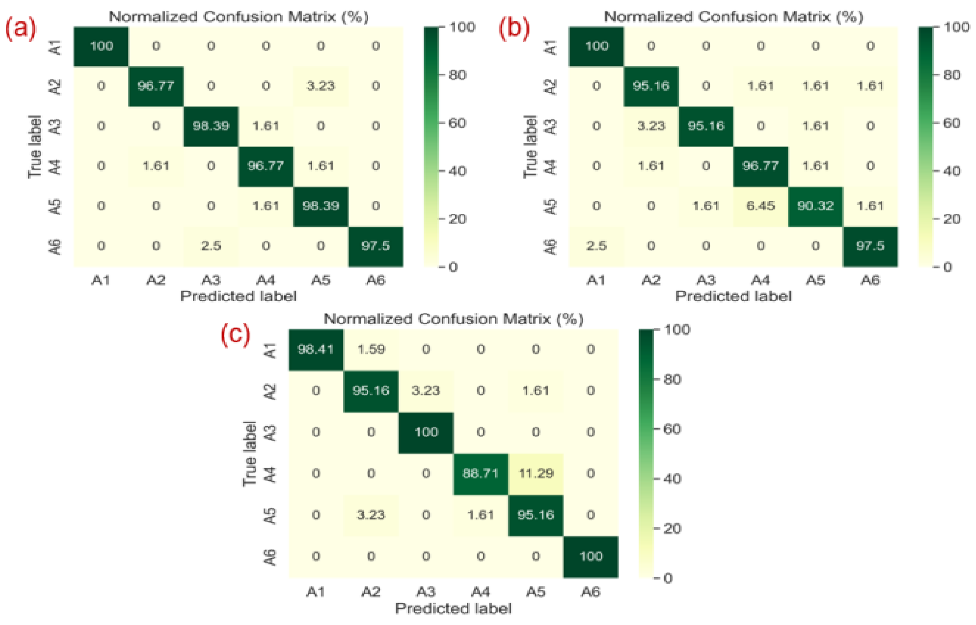
In this section, we will compare the performance metrics of the 12 MDPs (named M1, M2, M3, etc.), as described in Section 3.3.5, and the results are listed in Table 4. Based on these metrics, the M1, M7, and M10 pairs were selected from the 12-MDPs as the best performing pairs in terms of accuracy. The M1, M7, and M10 pairs achieved the highest recognition accuracy in their respective radar domains (TR, STFT, and SPWVD) when used as input, confirming their importance for radar-based HAR systems. To evaluate the classification performance of each class, the confusion matrices were analyzed. Figure 4 a, b, and c show the confusion matrices for pairs M1, M7, and M10 that perform best. In particular, pair M7 identified A6, representing fall activity, with 100% accuracy, whereas pairs M1 and M10 achieved 97.50% accuracy. The three pairs, except pair M10, detected the A1 class, which represents walking activity, with 100% accuracy and 98.41% for pair M10.

4.2. Comprehensive Performance Analysis on Radar Domains

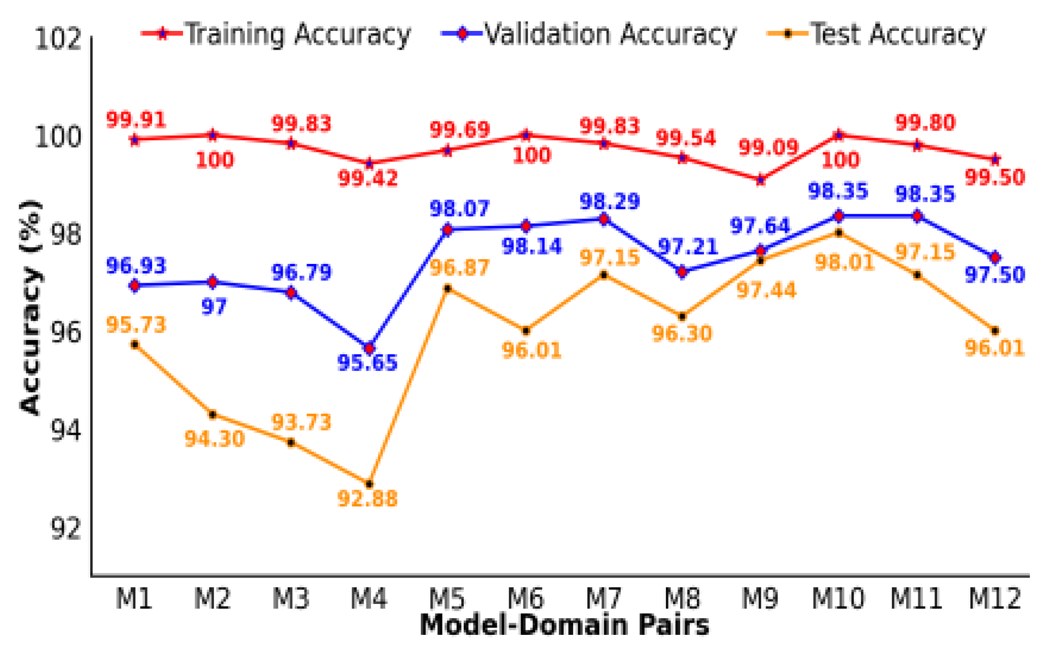
Evaluating the generalization ability of HAR systems is essential, particularly for limited datasets on radar-based human activity. Due to a lack of data, CNN classifiers tend to overfit. Therefore, it is important to evaluate the model’s performance on new, unseen radar data, which constitute the remaining 20% test set. The evaluation results of our HAR models are shown in Figure 5, showing consistent results, with the test accuracy showing the smallest variance between the 12 MDPs, as shown in Table 4.
From the Figure 5, the findings indicate that the models have strong generalization capabilities, with test accuracies ranging from 92.88% to 98.01%, confirming their effectiveness on the new data. Pair M10 achieved the highest test accuracy of 98.01%. On the other hand, although pairs M2 and M4 achieved perfect or near perfect average training accuracies of 100% and 99.42%, respectively, they had lower test accuracies of 94.30% and 92.88%, indicating that there is room for improvement. This difference highlights the importance of thorough testing of unseen data to accurately determine how well a model adapts to new input. The results emphasize the importance of using cross validation and remaining datasets for testing to evaluate the model generalization in real-world scenarios. Furthermore, choosing the best MDP requires a balanced evaluation of its performance, based on its generalization ability and computational efficiency.

4.3. Computational Efficient and LightWeight HAR Model

Computational efficiency is critical for real-time radar-based HAR system, particularly for resource-constrained edge devices. Therefore, it is crucial to develop a lightweight model that can quickly and accurately recognize human activities while minimizing the inference latency. This section examines computational efficiency using time metrics, such as training time and inference time as defined in Section 3.3.6, to evaluate the suitability of various models for real-world deployment, as detailed in Table 5. The fastest predicted pairs, M4, M8, and M12, were chosen based on inference time, an important metric for resource-constrained edge devices that require fast activity prediction.
The inference time is also defined as the time between initiating a prediction request and receiving the prediction output from the test model. This metric is very important for evaluating the performance and efficiency of a model, particularly in applications that require real-time processing on edge devices or standalone systems. Inference time directly affects the user experience and applicability of the model in time-sensitive scenarios, such as fall detection.

4.4. Computational Cost Across Radar Domains

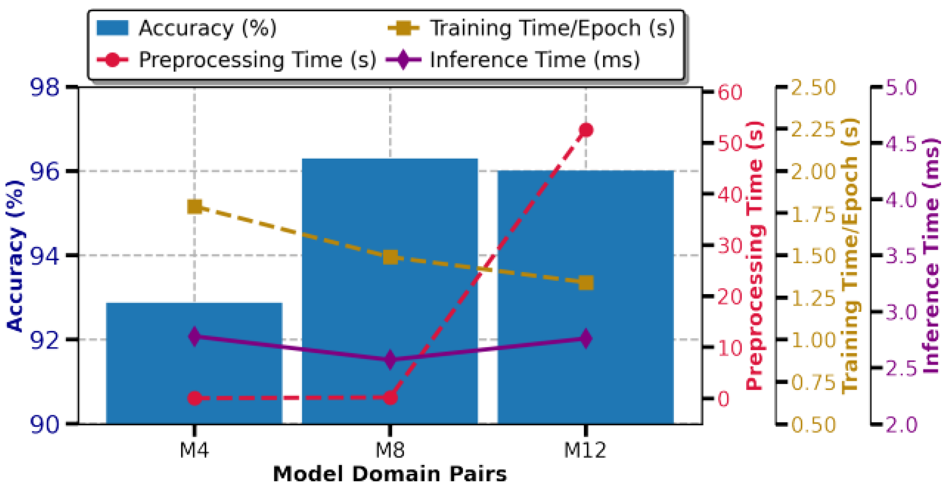
For the TR domain, the preprocessing time for processing the input raw radar data and visualizing an image representing the range over time as shown in Figure 3, is only 0.035 s, which is very low compared to other techniques illustrated in Figure 6. However, when inputted to a CNN model, it results in lower accuracy and higher computational cost. Among all models, MobileNetV2 (M4) exhibits the best training and inference efficiency, with a training time of 1.79 s/epoch, an inference time of 2.78 ms / sample and a recognition accuracy of 92.88% as shown in Figure 6. In contrast, the other three models are known for their higher accuracy, but with increased time measurements.
The STFT-based TD map shows the change in frequency over time (Doppler shift), as shown in Figure 3 and takes only 0.22 s to preprocess and generate a spectrogram using the STFT method. When this spectrogram is used as an input feature to the network, it provides a good balance between the performance and efficiency. For example, MobileNetV2 (M8) had a training time of 1.49 s/epoch and an inference time of 2.57 ms/sample, with a test accuracy of 96.30%. In contrast, VGG-16 and ResNet-50 achieved higher recognition accuracies of 96.87% and 97.15%, respectively, but had longer training and inference times, indicating higher resource usage illustrated in Tabel Table 4 and Table 5. On the other hand, VGG-19 has a longer prediction time of 6.90 ms/sample, making it less suitable for real-time systems.
Despite the lengthy preprocessing time of 52.58 s to generate a spectrogram using the SPWVD method, MobileNetV2 (M12) had a lower training time of 1.34 s/epoch and an inference time of 2.76 ms/sample with a recognition accuracy of 96.01% as shown in Figure 6, when SPWVD was used as input compared to the TR and STFT domains. This shows the advantage of higher resolution by combining both time and frequency windows simultaneously as detailed in Section 3.2.3. Despite the advantage, still SPWVD is not suitable for real-time systems due to the higher preprocessing time that require rapid preprocessing and prediction response, from data acquisition to model prediction specifically for critical activity like fall detection in elderly care homes.
This study concludes with two main possibilities for selecting the best model and radar domain for HAR systems. VGG-19 with SPWVD radar map performs well for applications that emphasize recognition accuracy, achieving a high recognition accuracy of 98.01% despite the longer preprocessing time. In contrast, for situations that require fast prediction, MobileNetV2 with STFT radar map is the most efficient, achieving the shortest inference time of 2.57 ms/sample while maintaining a remarkable accuracy of 96.30%, which is ideal for many real-time applications. Although TR maps provide consistent recognition accuracy across models, they often lag in inference time unless combined with MobileNetV2.
However, the study had limitations. A key challenge is the need for more studies on energy consumption, which is required to implement these models in resource-constrained edge devices. Future research should incorporate energy consumption measures to assess the suitability of each model and radar domain combination in low-power environments. In addition, further studies might look at how model reduction and optimization approaches, such as quantization and pruning, can improve the deployment potential of radar-based HAR systems on edge devices.

4.5. Comparison of Pair M8 with State-of-the-Art Models

A detailed comparative analysis is presented in Table 6. All models used STFT-based spectrogram inputs with a resolution of 224 × 224 pixels. The CNN [53], model trained from scratch achieved 95.44% accuracy, but the inference time per sample was 5.14 ms, which is almost twice that of our proposed MobileNetV2 model. The CNN + LSTM [23], model had the shortest training time per epoch of 1.12 s, but the accuracy was only 84.90%, and the inference time was as high as 6.04 ms/sample, almost three times that of our proposed model. The Bi-LSTM [42], model achieved a competitive accuracy of 95.16% with an inference time of 2.77 ms/sample, lagging behind the MobileNetV2 model in both training and inference time.
The proposed MobileNetV2 model, leveraging transfer learning, achieved the highest accuracy of 96.30% and the best inference time of 2.57 ms/sample, making it suitable for real-time applications. This shows that MobileNetV2 not only surpasses the accuracy of other state-of-the-art models trained from scratch but also significantly reduces inference time, providing an efficient option for real-time processing. This comparison highlights the adaptability and potential of our proposed work for a wide range of future applications, setting a benchmark for HAR systems in terms of both performance and efficiency.

5. Conclusions

In this study, we applied three preprocessing techniques, such as: Range-FFT for TR, STFT, and SPWVD, as inputs to CNN models for HAR and evaluated their computational efficiency for edge deployment, resulting in twelve different combinations of model-preprocessing pairs. These combinations include VGG-16, VGG-19, ResNet-50, and MobileNetV2 architectures. Among them, the combination of MobileNetV2 with STFT (model M8) showed balanced performance, setting a new benchmark for the state-of-the-art radar-based HAR system. This result emphasizes the importance of thorough evaluation of the entire process chain. The effectiveness of model M8 highlights its ability to support more advanced edge device models, which are typically associated with TinyML. Our work not only contributes to current methodologies but also lays the foundation for integrating more complex models into low-power, real-time edge systems.
Furthermore, in anticipation of advancements, our future research will focus on integrating neuromorphic federated learning and congestion-aware spiking neural networks to design energy-efficient systems, which is an important aspect not discussed in this study. This strategy aims to improve the real-time performance of radar-based HAR systems and address the trade-off between accuracy and energy efficiency.

Author Contributions

Conceptualisation, F.A., B.A. and A.Z.; methodology, F.A., B.A, S.H. and A.Z.; software, F.A.; validation, F.A., B.A., S.H and A.Z.; formal analysis, F.A., B.A., S.H. and A.Z.; writing original draft, F.H; writing, review and editing, F.A., B.A., S.H., M.A.I., K.A., K.A. and A.Z.; supervision, A.Z. All authors have read and agreed to the published version of the manuscript.

Data Availability Statement

This study is conducted using a publicly available datasets. Here is the link of the dataset: https://researchdata.gla.ac.uk/848/.

Acknowledgments

This Paper is supported by Ajman University Internal Research Grant No. 2024-IRG-ENIT-1. The research findings presented in this paper are solely the author(s)’ responsibility.

Conflicts of Interest

The authors declare no conflicts of interest.

References

  1. W. Jiao, R. Li, J. Wang, D. Wang, and K. Zhang, “Activity recognition in rehabilitation training based on ensemble stochastic configuration networks,” Neural Computing and Applications, vol. 35, no. 28, pp. 21229–21245, 2023.
  2. D. Deotale, M. Verma, P. Suresh, and N. Kumar, “Physiotherapy-based human activity recognition using deep learning,” Neural Computing and Applications, vol. 35, no. 15, pp. 11431–11444, 2023.
  3. N. Golestani and M. Moghaddam, “Human activity recognition using magnetic induction-based motion signals and deep recurrent neural networks,” Nature Communications, vol. 11, no. 1, pp. 1551, 2020.
  4. C.M. Ranieri, S. MacLeod, M. Dragone, P.A. Vargas, and R.A.F. Romero, “Activity recognition for ambient assisted living with videos, inertial units and ambient sensors,” Sensors, vol. 21, no. 3, pp. 768, 2021.
  5. H. Storf, T. Kleinberger, M. Becker, M. Schmitt, F. Bomarius, and S. Prueckner, “An event-driven approach to activity recognition in ambient assisted living,” in Proc. Ambient Intelligence: European Conference, AmI 2009, Salzburg, Austria, Nov. 18-21, 2009, pp. 123–132.
  6. A. Zam, A. Bohlooli, and K. Jamshidi, “Unsupervised deep domain adaptation algorithm for video-based human activity recognition via recurrent neural networks,” Engineering Applications of Artificial Intelligence, vol. 136, pp. 108922, 2024.
  7. A.C. Cob-Parro, C. Losada-Gutiérrez, M. Marrón-Romera, A. Gardel-Vicente, and I. Bravo-Muñoz, “A new framework for deep learning video-based human action recognition on the edge,” Expert Systems with Applications, vol. 238, pp. 122220, 2024.
  8. Y. Lu, L. Zhou, A. Zhang, S. Zha, X. Zhuo, and S. Ge, “Application of deep learning and intelligent sensing analysis in smart home,” Sensors, vol. 24, no. 3, pp. 953, 2024.
  9. E.K. Kumar, D.A. Kumar, K. Murali, P. Kiran, and M. Kumar, “Three stream human action recognition using Kinect,” in AIP Conference Proceedings, vol. 2512, no. 1, 2024.
  10. S. Zhang, Y. Li, S. Zhang, F. Shahabi, S. Xia, Y. Deng, and N. Alshurafa, “Deep learning in human activity recognition with wearable sensors: A review on advances,” Sensors, vol. 22, no. 4, pp. 1476, 2022.
  11. S. Mekruksavanich and A. Jitpattanakul, “Device position-independent human activity recognition with wearable sensors using deep neural networks,” Applied Sciences, vol. 14, no. 5, pp. 2107, 2024.
  12. X. Li, Y. He, and X. Jing, “A survey of deep learning-based human activity recognition in radar,” Remote Sensing, vol. 11, no. 9, pp. 1068, 2019.
  13. Y. Yao, W. Liu, G. Zhang, and W. Hu, “Radar-based human activity recognition using hyperdimensional computing,” IEEE Transactions on Microwave Theory and Techniques, vol. 70, no. 3, pp. 1605–1619, 2021.
  14. J. Yousaf, S. Yakoub, S. Karkanawi, T. Hassan, E. Almajali, H. Zia, and M. Ghazal, “Through-the-wall human activity recognition using radar technologies: A review,” IEEE Open Journal of Antennas and Propagation, 2024.
  15. S. Huan, L. Wu, M. Zhang, Z. Wang, and C. Yang, “Radar human activity recognition with an attention-based deep learning network,” Sensors, vol. 23, no. 6, pp. 3185, 2023.
  16. R. Yu, Y. Du, J. Li, A. Napolitano, and J. Le Kernec, “Radar-based human activity recognition using denoising techniques to enhance classification accuracy,” IET Radar, Sonar & Navigation, vol. 18, no. 2, pp. 277–293, 2024.
  17. F. Ayaz, B. Alhumaily, S. Hussain, L. Mohjazi, M.A. Imran, and A. Zoha, “Integrating millimeter-wave FMCW radar for investigating multi-height vital sign monitoring,” in Proc. 2024 IEEE Wireless Communications and Networking Conference (WCNC), pp. 1–6, 2024. [CrossRef]
  18. G. Paterniani, D. Sgreccia, A. Davoli, G. Guerzoni, P. Di Viesti, A.C. Valenti, M. Vitolo, G.M. Vitetta, and G. Boriani, “Radar-based monitoring of vital signs: A tutorial overview,” Proceedings of the IEEE, vol. 111, no. 3, pp. 277–317, 2023. [CrossRef]
  19. S. Iyer, L. Zhao, M.P. Mohan, J. Jimeno, M.Y. Siyal, A. Alphones, and M.F. Karim, “mm-Wave radar-based vital signs monitoring and arrhythmia detection using machine learning,” Sensors, vol. 22, no. 9, pp. 3106, 2022.
  20. L. Qu, Y. Wang, T. Yang, and Y. Sun, “Human activity recognition based on WRGAN-GP-synthesized micro-Doppler spectrograms,” IEEE Sensors Journal, vol. 22, no. 9, pp. 8960–8973, 2022. [CrossRef]
  21. X. Li, Y. He, F. Fioranelli, and X. Jing, “Semisupervised human activity recognition with radar micro-Doppler signatures,” IEEE Transactions on Geoscience and Remote Sensing, vol. 60, pp. 1–12, 2022. [CrossRef]
  22. W.-Y. Kim and D.-H. Seo, “Radar-based HAR combining range–time–Doppler maps and range-distributed-convolutional neural networks,” IEEE Trans. on Geoscience and Remote Sensing, vol. 60, pp. 1–11, 2022. [CrossRef]
  23. W. Ding, X. Guo, and G. Wang, “Radar-based human activity recognition using hybrid neural network model with multidomain fusion,” IEEE Transactions on Aerospace and Electronic Systems, vol. 57, no. 5, pp. 2889–2898, 2021. [CrossRef]
  24. Z. Liu, L. Xu, Y. Jia, and S. Guo, “Human activity recognition based on deep learning with multi-spectrogram,” in Proc. 2020 IEEE 5th International Conference on Signal and Image Processing (ICSIP), pp. 11–15, 2020.
  25. Y. Qian, C. Chen, L. Tang, Y. Jia, and G. Cui, “Parallel LSTM-CNN network with radar multispectrogram for human activity recognition,” IEEE Sensors Journal, vol. 23, no. 2, pp. 1308–1317, 2022.
  26. Y. LeCun, L. Bottou, Y. Bengio, and P. Haffner, “Gradient-based learning applied to document recognition,” Proceedings of the IEEE, vol. 86, no. 11, pp. 2278–2324, 1998.
  27. A. Krizhevsky, I. Sutskever, and G.E. Hinton, “Imagenet classification with deep convolutional neural networks,” Advances in Neural Information Processing Systems, vol. 25, 2012.
  28. A. Alkasimi, A.-V. Pham, C. Gardner, and B. Funsten, “Human activity recognition based on 4-domain radar deep transfer learning,” in Proc. 2023 IEEE Radar Conference (RadarConf23), pp. 1–6, 2023.
  29. A. Dixit, V. Kulkarni, and V.V. Reddy, “Cross frequency adaptation for radar-based human activity recognition using few-shot learning,” IEEE Geoscience and Remote Sensing Letters, 2023.
  30. O. Pavliuk, M. Mishchuk, and C. Strauss, “Transfer learning approach for human activity recognition based on continuous wavelet transform,” Algorithms, vol. 16, no. 2, pp. 77, 2023.
  31. D. Theckedath and R.R. Sedamkar, “Detecting affect states using VGG16, ResNet50 and SE-ResNet50 networks,” SN Computer Science, vol. 1, pp. 1–7, 2020. [Online]. Available online: https://link.springer.com/article/10.1007/s42979-020-0114-9.
  32. N. Dey, Y.-D. Zhang, V. Rajinikanth, R. Pugalenthi, and N.S.M. Raja, “Customized VGG19 architecture for pneumonia detection in chest X-rays,” Pattern Recognition Letters, vol. 143, pp. 67–74, 2021.
  33. M. Sandler, A. Howard, M. Zhu, A. Zhmoginov, and L.-C. Chen, “MobileNetV2: Inverted residuals and linear bottlenecks,” in Proc. IEEE Conference on Computer Vision and Pattern Recognition, pp. 4510–4520, 2018.
  34. F. Kulsoom, S. Narejo, Z. Mehmood, H. N. Chaudhry, A. Butt, and A. K. Bashir, “A review of machine learning-based human activity recognition for diverse applications,” Neural Computing and Applications, vol. 34, no. 21, pp. 18289–18324, 2022.
  35. A. Biswal, S. Nanda, C. R. Panigrahi, S. K. Cowlessur, and B. Pati, “Human activity recognition using machine learning: A review,” in Progress in Advanced Computing and Intelligent Engineering: Proceedings of ICACIE 2020, pp. 323–333, 2021.
  36. M. Zenaldin and R. M. Narayanan, “Radar micro-Doppler based human activity classification for indoor and outdoor environments,” in Radar Sensor Technology XX, vol. 9829, pp. 364–373, 2016.
  37. L. Tang, Y. Jia, Y. Qian, S. Yi, and P. Yuan, “Human activity recognition based on mixed CNN with radar multi-spectrogram,” IEEE Sensors Journal, vol. 21, no. 22, pp. 25950–25962, 2021.
  38. F. J. Abdu, Y. Zhang, and Z. Deng, “Activity classification based on feature fusion of FMCW radar human motion micro-Doppler signatures,” IEEE Sensors Journal, vol. 22, no. 9, pp. 8648–8662, 2022.
  39. A. Shrestha, C. Murphy, I. Johnson, A. Anbulselvam, F. Fioranelli, J. Le Kernec, and S. Z. Gurbuz, “Cross-frequency classification of indoor activities with dnn transfer learning,” in 2019 IEEE Radar Conference (RadarConf), pp. 1–6, 2019.
  40. Z.A. Sadeghi and F. Ahmad, “Whitening-aided learning from radar micro-Doppler signatures for human activity recognition,” Sensors, vol. 23, no. 17, pp. 7486, 2023.
  41. X. Zhou, J. Tian, and H. Du, “A lightweight network model for human activity classification based on pre-trained MobileNetV2,” in IET Conference Proceedings CP779, vol. 2020, no. 9, pp. 1483–1487, 2020.
  42. A. Shrestha, H. Li, J. Le Kernec, and F. Fioranelli, “Continuous human activity classification from FMCW radar with Bi-LSTM networks,” IEEE Sensors Journal, vol. 20, no. 22, pp. 13607–13619, 2020.
  43. F. Fioranelli et al., “Radar signatures of human activities,” Univ. Glasgow, Glasgow, U.K., 2019. [Online]. Available online: https://researchdata.gla.ac.uk/848/.
  44. S. Yang, et al., “The Human Activity Radar Challenge: Benchmarking Based on the ‘Radar Signatures of Human Activities’ Dataset From Glasgow University,” IEEE Jr. Biomedical and Health Informatics, vol. 27, 2023.
  45. A. Safa, F. Corradi, L. Keuninckx, I. Ocket, A. Bourdoux, F. Catthoor, and G. G. E. Gielen, “Improving the Accuracy of Spiking Neural Networks for Radar Gesture Recognition Through Preprocessing,” IEEE Transactions on Neural Networks and Learning Systems, vol. 34, no. 6, pp. 2869–2881, 2023. [CrossRef]
  46. J. Deng, W. Dong, R. Socher, L. Li, K. Li, and L. Fei-Fei, “Imagenet: A large-scale hierarchical image database,” in 2009 IEEE Conference on Computer Vision and Pattern Recognition, pp. 248–255, 2009.
  47. K. Simonyan and A. Zisserman, “Very deep convolutional networks for large-scale image recognition,” arXiv preprint arXiv:1409.1556, 2014.
  48. A. Faghihi, M. Fathollahi, and R. Rajabi, “Diagnosis of skin cancer using VGG16 and VGG19 based transfer learning models,” Multimedia Tools and Applications, vol. 83, no. 19, pp. 57495–57510, 2024.
  49. Z. Wu, C. Shen, and A. Van Den Hengel, “Wider or deeper: Revisiting the resnet model for visual recognition,” Pattern Recognition, vol. 90, pp. 119–133, 2019.
  50. A. G. Howard, “Mobilenets: Efficient convolutional neural networks for mobile vision applications,” arXiv preprint arXiv:1704.04861, 2017.
  51. M. Sandler, A. Howard, M. Zhu, A. Zhmoginov, and L.-C. Chen, “Mobilenetv2: Inverted residuals and linear bottlenecks,” in Proceedings of the IEEE Conference on Computer Vision and Pattern Recognition, pp. 4510–4520, 2018.
  52. S. Takano, “Chapter 2 - traditional microarchitectures,” in Thinking machines, S. Takano, Ed. Academic Press, 2021, pp. 19–47.
  53. K. Papadopoulos and M. Jelali, “A Comparative Study on Recent Progress of Machine Learning-Based Human Activity Recognition with Radar,” Applied Sciences, vol. 13, no. 23, pp. 12728, 2023.
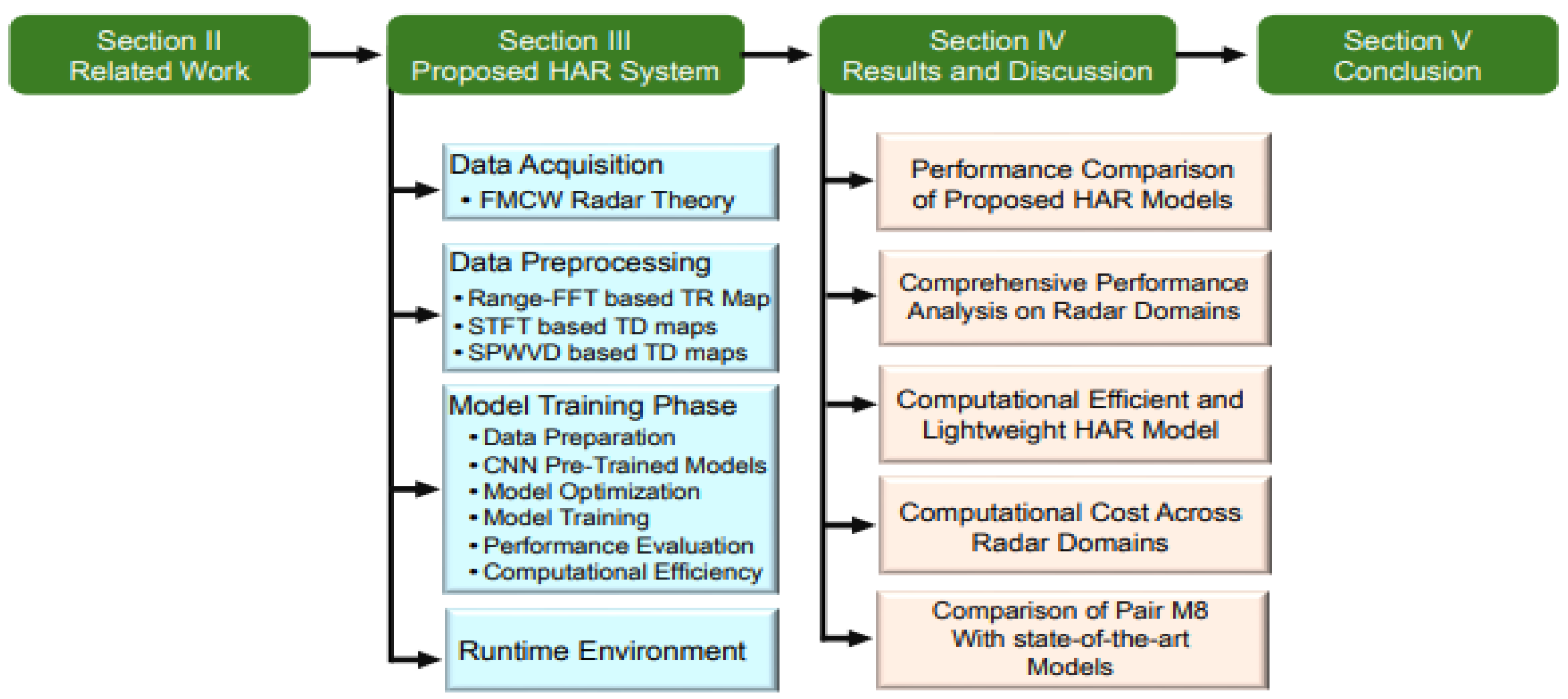
Figure 1. Detailed flow diagram illustrating the structure of the paper sections and content.
Preprints 142084 g001
Figure 2. Radar-based HAR system depicting the workflow from data acquisition to radar maps generation, along with state-of-the-art Neural Networks.
Preprints 142084 g002
Figure 3. 2D images of six activities resulting from TR, STFT and SPWVD techniques.
Preprints 142084 g003
Figure 4. Confusion matrices of best performing pairs. (a) shows pair M1, (b) shows pair M7 and (c) shows pair M10.
Preprints 142084 g004
Figure 5. Generalization capability of the proposed HAR system.
Preprints 142084 g005
Figure 6. Performance and computational analysis comparison across radar domains as input to MobileNetV2.
Preprints 142084 g006
Table 1. Comparison of key characteristics and attributes among existing state-of-the-art radar-based HAR studies.
Ref. Radar Domains Data Preprocessing CNN/LSTM TL-Based
TR STFT SPWVD Time methods
[15]
[22]
[23]
[24]
[25]
[37]
[40]
[41]
[42]
Our
Table 2. Details of Human Activity classes.
Short Name Activity Description Samples Duration
A1 Walking back and forth 312 10 s
A2 Sitting on a chair 311 5 s
A3 Standing 311 5 s
A4 Bend to pick an object 309 5 s
A5 Drinking water 311 5 s
A6 Fall 197 5 s
Table 3. Pre-trained CNN hyperparameters.
Parameters VGG-16 VGG-19 ResNet-50 MobileNetV2
Batch size 32 32 32 32
Dropout 0.5 0.2 0.2 0.2
Learning rate 2e-3 2e-3 2e-3 4e-4
Optimizer SGD SGD SGD Adam
Decay - 1e-6 1e-6 -
Momentum 0.9 0.9 0.9 -
Epochs/Fold 25 25 25 25
Table 4. Comparison of Evaluation Metrics for Proposed HAR Models across Radar Domains.
MDPs Radar Domains Models Accuracy (%) Precision Recall F1-score
M1 TR VGG-16 95.73 0.9576 0.9573 0.9572
M2 TR VGG-19 94.30 0.9436 0.9430 0.9429
M3 TR ResNet-50 93.73 0.9373 0.9373 0.9368
M4 TR MobileNetV2 92.88 0.9307 0.9288 0.9284
M5 STFT VGG-16 96.87 0.9697 0.9687 0.9687
M6 STFT VGG-19 96.01 0.9639 0.9624 0.9624
M7 STFT ResNet-50 97.15 0.9721 0.9731 0.9721
M8 STFT MobileNetV2 96.30 0.9635 0.9651 0.9642
M9 SPWVD VGG-16 97.44 0.9764 0.9744 0.9745
M10 SPWVD VGG-19 98.01 0.9803 0.9801 0.9801
M11 SPWVD ResNet-50 97.15 0.9720 0.9715 0.9715
M12 SPWVD MobileNetV2 96.01 0.9629 0.9580 0.9600
Table 5. Comparison of training and inference times for computational efficiency across 12-MDPs.
Model-Domain Training Inference
Pairs Time/epoch (s) Time/sample (ms)
M1 3.40 7.16
M2 3.77 8.11
M3 2.77 3.80
M4 1.79 2.78
M5 3.38 7.10
M6 4.38 6.90
M7 2.74 3.54
M8 1.49 2.57
M9 3.50 7.02
M10 3.76 6.88
M11 2.73 3.99
M12 1.34 2.76
Table 6. Time metrics and accuracy comparison of proposed lightweight model against alternative approaches.
Ref. Models Training Inference Accuracy
Time/epoch (s) Time/sample (ms) (%)
[23] CNN+LSTM 1.12 6.04 84.90
[42] Bi-LSTM 1.70 2.77 95.16
[53] CNN 1.88 5.14 95.44
Our Pair M8 1.49 2.57 96.30
Disclaimer/Publisher’s Note: The statements, opinions and data contained in all publications are solely those of the individual author(s) and contributor(s) and not of MDPI and/or the editor(s). MDPI and/or the editor(s) disclaim responsibility for any injury to people or property resulting from any ideas, methods, instructions or products referred to in the content.
Copyright: This open access article is published under a Creative Commons CC BY 4.0 license, which permit the free download, distribution, and reuse, provided that the author and preprint are cited in any reuse.
Prerpints.org logo

Preprints.org is a free preprint server supported by MDPI in Basel, Switzerland.

Subscribe

© 2024 MDPI (Basel, Switzerland) unless otherwise stated