Assessment of the Representativeness and Uncertainties of CTD Temperature Profiles

Preprint

Article

Assessment of the Representativeness and Uncertainties of CTD Temperature Profiles

Altmetrics

Downloads

Views

Comments

This version is not peer-reviewed

Submitted:

05 December 2024

Posted:

09 December 2024

You are already at the latest version

Alerts

Abstract

CTD profilers are used as reference instruments to qualify temperature and salinity data. Their metrological specifications can be controlled in calibration bath and calibration coefficients can be applied to correct the linearity of sensors and the trueness of measured data with a given uncertainty. However, in ocean areas with thermal gradients, the uncertainty of the measured data is questionable due to the thermal inertia of sensors and the movements of the CTD, in relation with the roll or pitch of the boat. In order to evaluate these measurement uncertainties and in order to be able to use the upcast profiles, a double C-T sensors SBE 9 profiler was fixed under a carousel water sampler, the second C-T couple being at the top of the carousel frame. This configuration allows the evaluation of temperature measurement deviations of recorded profiles. In order to quantify the different sources of instrumental uncertainties, the temperature signal has been modelled accounting for the movements induced by the boat. The result allows to quantify what can be called the representativeness of CTD’s temperature measurements. This notion is very useful in data assimilation process. A table quantifying the various sources of uncertainty has been created from profiles obtained during four offshore campaigns. In the future, it could be used to find the representativeness of similar profiles obtained with a single pair of sensors.

Keywords:

Subject: Environmental and Earth Sciences - Oceanography

1. Introduction

CTD profilers were design to respond to the World Ocean Circulation Experiments (WOCE) programme. It suggested that the quantities temperature and conductivity should be measured respectively to 0.002 °C and 0.002 mS cm⁻¹, resulting in a salinity measurement accuracy of ± 0.002 [1]. Le Menn [2] showed that if the uncertainty of ± 0.002 °C can be kept in calibration bath, the expanded uncertainty of calculated practical salinity was closed to ± 0.003.

Therefore, ship-based CTD profiles are used as reference to qualify temperature and salinity data from other instruments like XBT [3], ARGO floats [4] or marine mammal data loggers [5], using collocated profiles. CTD profiler’s metrological specifications can be controlled in calibration bath and calibration coefficients can be applied to correct the linearity of sensors and the trueness of measured data.

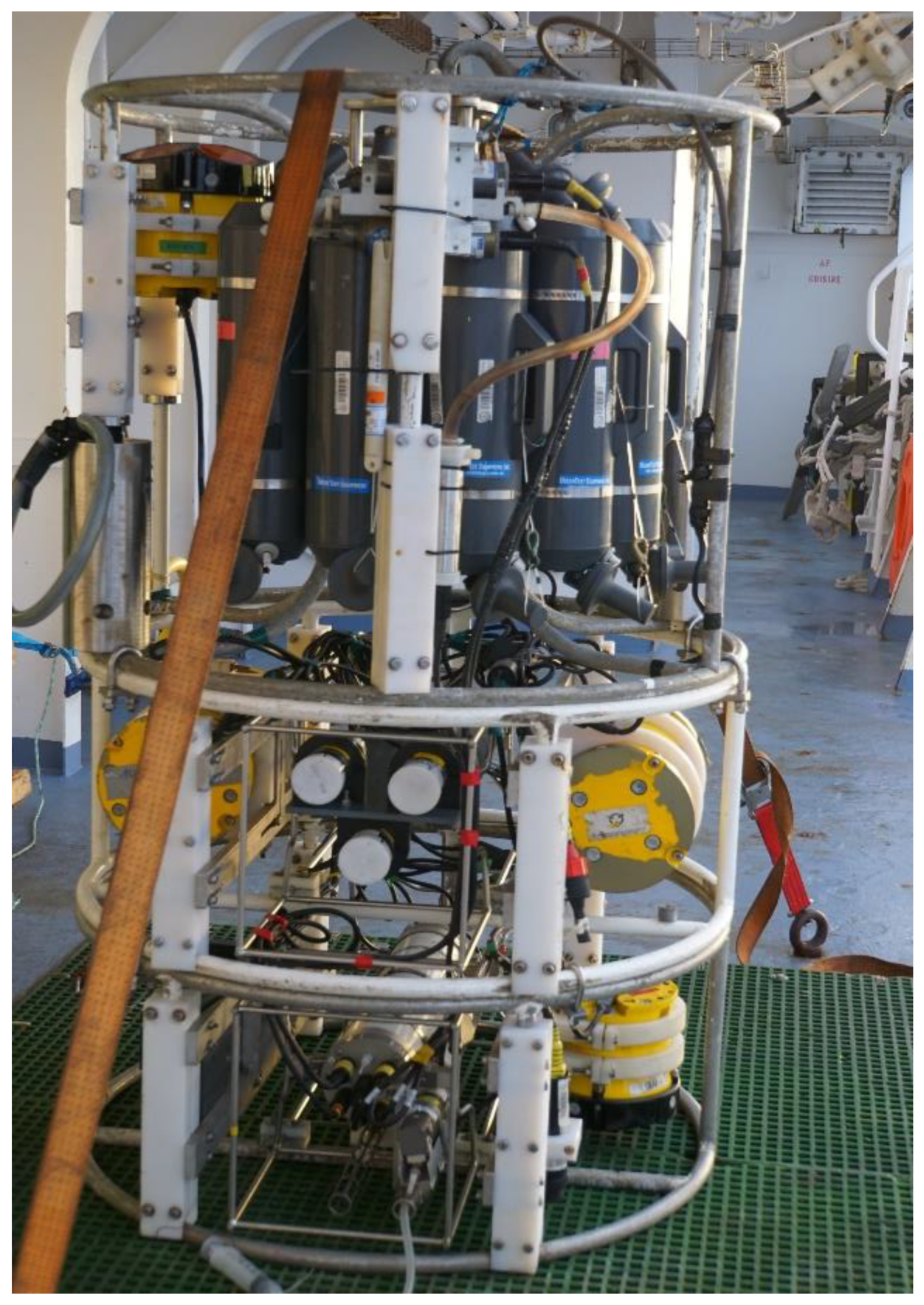
When used at sea, they are fixed generally on the bottom of a carousel water sampler frame (See Figure 1). This equipment is lowered at different depths, depending on the depth of the seafloor, thanks to a trawl. This configuration makes it possible to exploit the conductivity-temperature (C-T) profiles obtained during downcasts. In order to exploit the upcast profiles by avoiding the water mixing led in the carousel water sampler, the idea came to fix another C-T pair at the top of the carousel. This innovative configuration also opens the possibility to assess the natural variability of the medium in temperature between the downcast and the upcast, to the variable time scale of measurements (10 min to several hours). With properly calibrated sensors, in a quiet and homogeneous medium, this difference might be close to the calibration uncertainty or in the best cases, to the resolution of the instrument. But, profiles acquired during different campaigns at sea showed that this case is rarely met; several factors in relation with the natural variability and the instrument, make that deviations observed.

If the measurement uncertainty of the instrument in relation with its calibration, its sensors specifications and its drift in time can be evaluated, the remaining differences can be used to quantify the natural variability during the time of the down-up profile. This quantification can be used to describe the representativeness of temperature measurements at different depths, at the location of the profile.

Representativeness has been the subject of several different definitions. In 1981 Nappo et al. [6] defined it as “the extent to which a set of measurements taken in a given space-time domain reflect the actual conditions in the same or different space-time domain”. This definition is similar to the definition of reproducibility given in the International vocabulary of metrology or VIM [7], and corresponds fairly well to the notion of representativeness of the CTD profiles as we try to assess it in this publication. It is also close to the one given by R. Cooley et al. in 2020 [8] for whom representativeness can be defined purely in terms of the ability of the observational sampling to resolve the spatiotemporal scales of interest, which is entirely independent of measurement/instrument error. According to them it is also in relation with the error component associated with the representativeness of a single observation for a certain application.

Therefore, the notion and the definition of representativeness presents a great interest in data assimilation with optimal estimation [9,10,11]. Since the 80’th, the literature on this subject is abundant, and we will just focus on some recent publications that have tried to explain the use of this concept. In 2015, Hodyss et al. [12] defined it as the inability of a forecast model to accurately simulate the climatology of the truth. This very general definition illustrates the fact that it is difficult to discern the sources of errors in forecast models. In this representation, “the truth” refers to the observation point which is considered to have a neglecTable uncertainty and which is considered to see the small scales process, so that the model achieves relatively coarser states. In fact, the representativeness error also called representation error (RE), includes the measurement errors and the representation errors obtained by numerical models, and it describes the uncertainty of using a single measurement to represent the gridded averages for a certain spatial and temporal resolution.

In 2008, Oke and Sakov [13] defined the representativity as the component of observation error due to unresolved scales and processes, and they consider that the main source of RE is due to the limited (spatial and temporal) resolution of available observations. Their results suggest that the values of REs are typically greater than or at least comparable to measurement errors, particularly in regions of strong mesoscale variability [14]. This description was taken up by Janji’c et al., in 2018 [10]. However, according to them, the observation error has two components, the representation error which depends on how the measurements are used, for example in a data assimilation process, and the measurement error which is associated with the measurement device alone. In this description, the natural variability around the device during the data acquisition is basically ignored.

RE is also dependent on eddy activity according to Schiller et al. [15]. Efforts are made to improve forecasts in ocean eddies because, according to Rykova [16], the misfits between observations and analyses from high-resolution ocean forecast systems are large. She quantified this mis-fits between observed and analyzed fields to be 0.4 – 0.9 °C for subsurface temperature, 0.06 – 0.16 for subsurface salinity and 0.2 – 0.6 °C for sea surface temperature, so that measurement errors are given to be 0.004 °C for subsurface temperature and 0.01 for subsurface salinity for Argo profilers.

With the double CTD sensors configuration described in Section 2, we have the possibility to quantify the representativity or the degree of trueness of single profiles and of groups of profiles, to have a better assessment of the measurement error and of the natural variability during the measurements, per oceanic areas and to determine if this error is really neglecTable or of the same order that the observation error as defined by Oke and Sakov. It is assumed generally that REs are horizontally uniform and only depth dependent [16]. This hypothesis could also be tested by considering the measurement uncertainties of measured temperatures. An analysis of measurement uncertainties is developed in Section 3, to determine the origin of deviations between downcast and upcast. This uncertainty budget accounts for the location in depth of temperature measurements and the effects of sensors response time. We hope that this approach will allows a better understanding of the existing deviations between observed and analysed fields. For that, and to evaluate the uncertainties in relation with the response time, we developed a numerical model of the measured temperature that was used to simulate profiles obtained during different campaigns at sea. This model includes the effects of the boat’s movements. It is developed in Section 4 and Section 5 and the results are presented in Section 6, based on two examples of profiles. The Section 7 is a short description of campaigns locations, used in this study. A discussion of these results is made in Section 8, with the perspectives they offer.

2. The Experimental Apparatus

Measurements at sea are made with a carousel water sampler with a double frame under it (see Figure 1). The frame at the bottom contains a CTD profiler SBE 9⁺ fixed in a horizontal position. This CTD contains the first CT pair (SBE 3 and SBE 4 sensors from Sea-Bird Scientifics) used to measure temperature – conductivity data during the descent of the carousel. The water is pumped from a hose, the end of which is fixed to the lowest part of the frame. The second CT pair is fixed to the frame of the sample bottle rosette, along with a second pump. The water is drawn in at the same level as the top of the frame.

SBE 3 and SBE 4 sensors are calibrated before and after the campaigns with the SBE 9⁺ that will be and was used during the campaign to respectively ± 0.002 °C in the range 0 °C – 32 °C and ± 0.004 mS/cm in the range 0 mS/cm to 60 mS/cm. For the SBE 4 sensors, the calibration uncertainty can be higher according to the linearity and the reproducibility of its measurements in the bath, but it is never higher than ± 0.006 mS/cm. This study is focused mostly on temperature profiles. The drift over time of each sensor is known and can be quantify using a calibration correction history.

3. The Measurements Uncertainties of Temperature Measurements

The sensitive elements of SBE 3 sensors are thermistors. Thermistors have a non-linear response corrected with the Bennett formula and coefficients given in Sea Bird calibration reports. After using these coefficients, the remaining linearity uncertainty u_l is less than 0.1 mK [17]. This uncertainty appears like a residual Gaussian noise.

As thermistors are resistive sensors, they are fed by a current; another source of uncertainty is thus the self-heating created by the Joule effect. To reduce it, manufacturers use very small currents to fed the thermistor. Sea bird warrants a self-heating error inferior to 0.1 mK in still water for the SBE 3 sensor [17]. Since the only knowledge we have of this uncertainty u_sh is its maximum value, we can assign it a rectangular distribution.

Sea-Bird Scientific warrants an initial temperature accuracy of 0.002 °C. That can be considered as an expanded calibration uncertainty. It can be reached between - 1 °C and 32 °C with a very sTable calibration bath and a reference sensor regularly calibrated in fixed points cells of the International Temperature Scale of 1990 (ITS-90), regularly linked to the references of National Metrology Institutes. Considering these constraints, in this assessment the standard calibration uncertainty u_c, will be considered to be 1 mK.

At depth, pressure can compress the needle which sheltered the thermistor. Several assessments of this effect have been made. From in situ comparisons of SBE 3 and SBE 35, Uchida et al. concluded in 2007 that three probes were not very sensitive to pressure and eight had errors of 1 to 2 mK at a pressure of 600 bar [18]. In another study made in 2015, Uchida et al. have found one SBE 3 with an error of - 0.06 mK at 600 bar and another one (already tested in 2007) with an error of 5.07 mK instead of 1.94 mK in situ [19]. In 2017, experiments made in a pressure chamber on one SBE 3 have shown a sensitivity of – 77 μK MPa^-1 from 0.1 to 60 MPa [20]. That is equivalent to an error of – 4.6 mK at 600 bar. Therefore, it appears that the pressure sensitivity of SBE 3 is variable from one probe to the other and varies from neglecTable to 5 mK at 600 bar. The SBE 3 used during our measurements have never been tested in pressure. The maximal uncertainty led by the pressure effect is then u_p = 8 μK bar^-1. According to the Guide to the expression of uncertainty in measurement [21], the standard uncertainty of this effect can be evaluated to be 4.8 μK bar^-1 or 2.9 mK at 600 bar.

The acceleration of flow as it meets the surface of the sensor provokes an increase in temperature related to the fluid viscosity. This effect has been studied and quantified by Larson and Pedersen in 1996 [22]. According to their communication, the viscous heating uncertainty can be assessed with the relation dt = 1.263x10^-4 Pr^0.5U² where Pr is the Prandlt number and U the speed of the flow. If U = 1 m s^-1, dt  1 mK. If the flow changes or is not the same between the calibration and the using, this uncertainty should be considered. As it cannot be corrected, it corresponds to a standard uncertainty u_v of 1 mK.

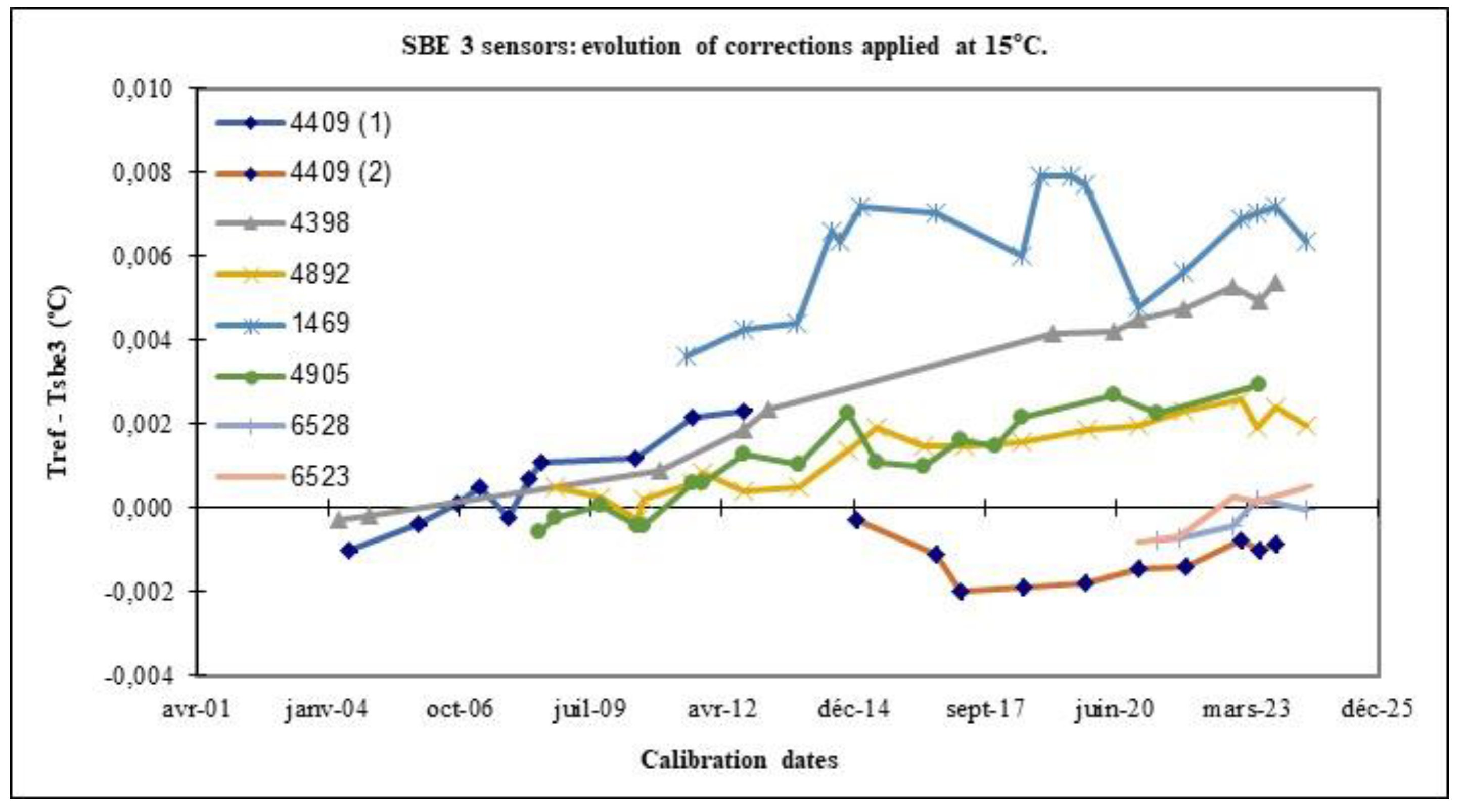
The drift over time of sensors between two calibrations must also be considered in the uncertainty budget. Figure 2 presents the drift of SBE 3 sensors used in this study. Explanations of how these drifts are obtained can be found in reference [23]. It is generally very low: between 6 μK/year (sn 4409(2)) and 0.29 mK/year at 15 °C for the older SBE 3 (sn 4398 and 4409(1)). However, depending on use, the drift between 2 calibrations may be greater. For example: the sn 6528 (pale blue) used in hard conditions, on a towed fish SeaSoar. For more information about the using of this towed fish, see the reference [24]. This one was not used for the double sensor measurements. The drift uncertainty u_d can be considered to be 0.29 mK/year, with a maximum time between two calibrations of 12 months.

During temperature measurements at sea and particularly as the sensor passes through temperature gradients, another parameter can introduce measurement uncertainties: the depth positioning. This uncertainty depends on the pressure sensor measurement trueness. A true depth positioning is mandatory to follow the evolution of the thermal contain of oceans. For the World Ocean Circulation Experiments (WOCE) the specification is 1 dbar at 6000 dbar. At low depth, constraints are more important because of temperature gradients and thus not well defined. The resolution and accuracy of pressure sensors decrease as their measurement range increases. SBE 9⁺ are equipped with Piezoelectric sensors Digiquartz of ParoScientific. These sensors have a very good repeatability of 0.005 % of the full scale, corresponding to a standard uncertainty u_r = 0.34 dbar for a 6800 dbar range. Their thermal sensitivity is 0.0008 % of the full scale °C^-1. With a thermal variation range of ± 20 °C that makes an uncertainty: u_Ts = 0.98 dbar. Their initial accuracy is ± 0.015 % or ≈ 1.02 dbar for a 6800 dbar range and their typical stability is ± 0.02 % per year. That can be considered as a maximal drift uncertainty u_d. For one annual calibration, it corresponds to ≈ 1.4 dbar/year (6800 dbar).

However, with an automated pressure balance as the PG7502 of the manufacturer Fluke Calibration, it is possible to obtain a calibration standard uncertainty u_c = 0.2 dbar. The pressure sensor’s drift of the SBE 9⁺ sn 766 used on our carousel is 0.25 dbar year^-1.

In the case of the error curves that can be obtained with the double sensor measurements, this uncertainty is cancelled out to the nearest error due to sensor hysteresis. The typical hysteresis of a Digiquartz is 0.005 % of the full scale or 0.34 dbar, but measurements with a pressure balance show that this number is rarely met. For the SBE 9⁺ sn 766 used on our carrousel, the hysteresis standard uncertainty was evaluated to be u_h = 0.02 dbar (Students distribution with 5 degrees of freedom). 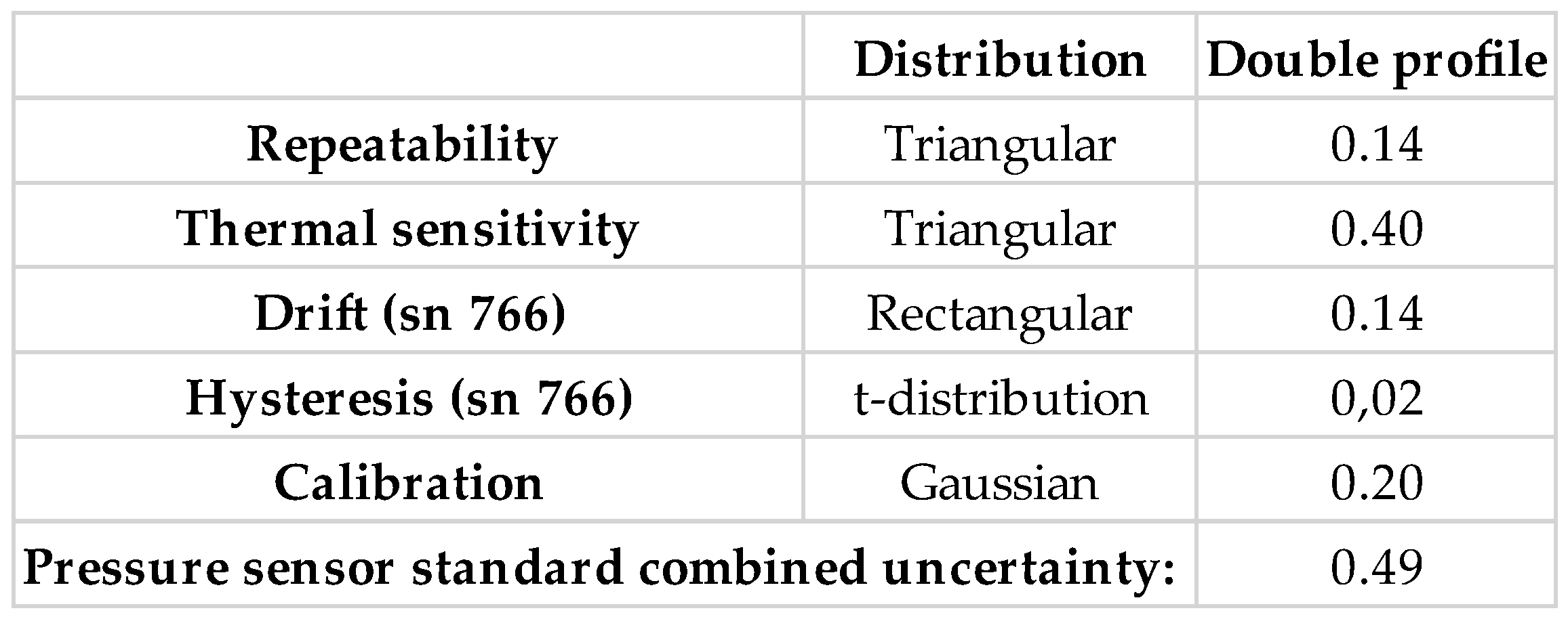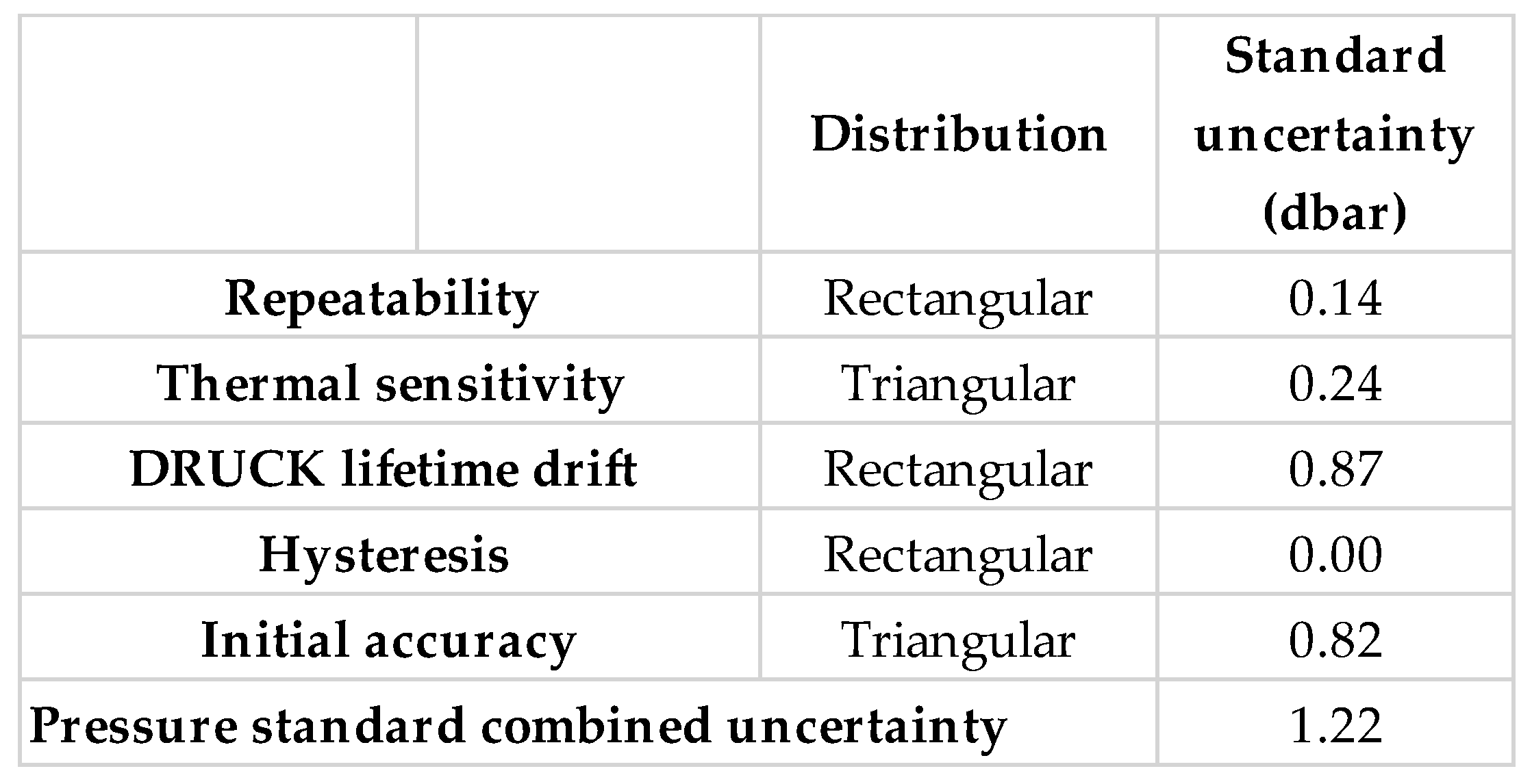Table 1 gives the standard uncertainty budget of the SBE 9⁺ sn 766 pressure sensor in the case of a single downward profile and in the case of the double sensor configuration. As the influence quantities are independent of each other, the combined standard uncertainty on the pressure measurements u_c(p) is obtained by a simple quadratic sum:

u_{c} (p) = \sqrt{{(\frac{u_{r}}{\sqrt{6}})}^{2} + {(\frac{u_{T s}}{\sqrt{6}})}^{2} + {(\frac{u_{d}}{\sqrt{3}})}^{2} + u_{h}^{2} + u_{c}^{2}}

(1)

The last uncertainty to evaluate is in relation with the response time of the temperature sensor. This uncertainty called u_ is studied in details in Section 4. Considering the details given in this Section, the combined standard uncertainty on temperature measurements can be assessed by the Equation (2):

u_{c} (T) = \sqrt{u_{l}^{2} + {(\frac{u_{s h}}{\sqrt{3}})}^{2} + u_{c}^{2} + u_{v}^{2} + {(\frac{u_{d}}{\sqrt{3}})}^{2} + {(\frac{u_{p} x p}{\sqrt{3}})}^{2} + {(u_{c} (p) x g r a d (T))}^{2} + u_{τ}^{2}}

(2)

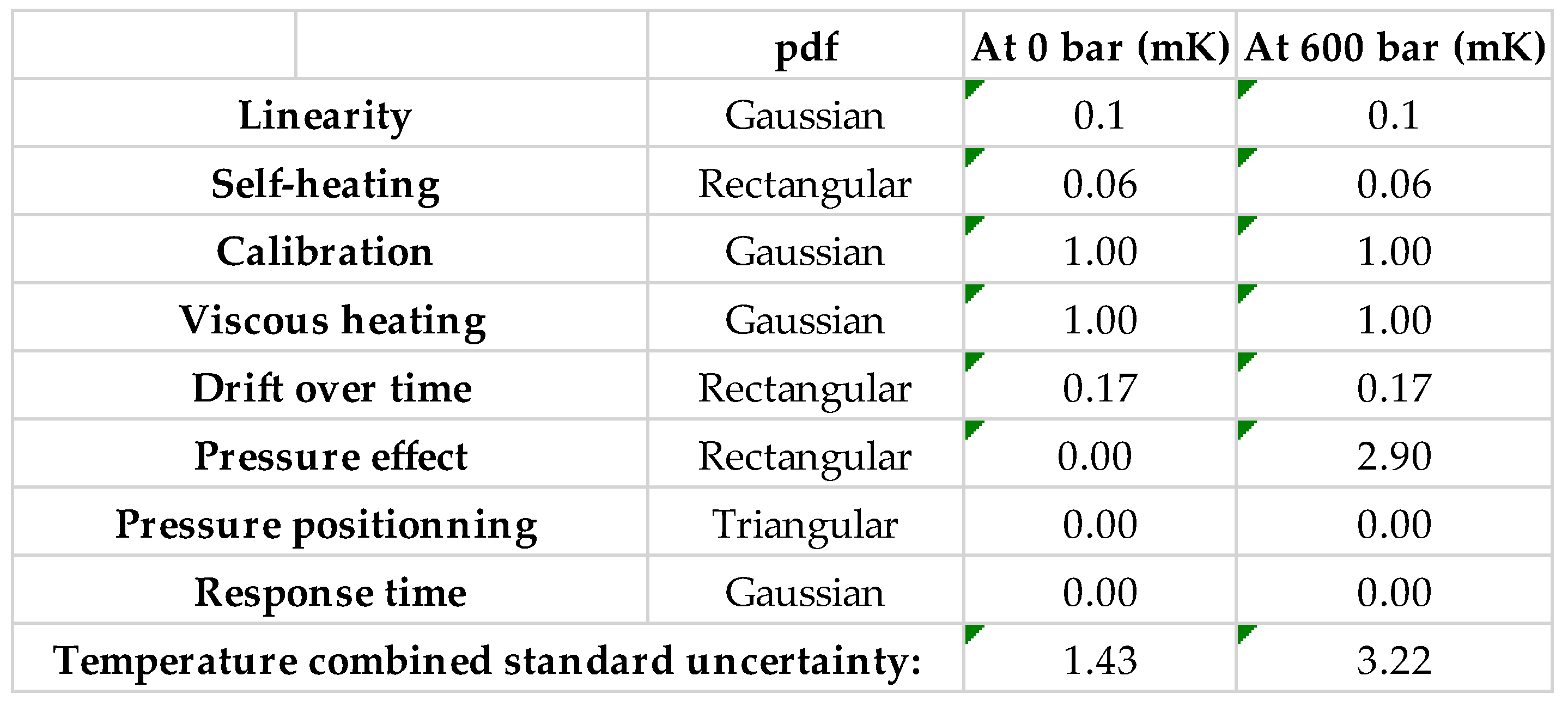
To conclude this Section, the uncertainty budget of SBE 9⁺ temperature measurements is largely dominated by the uncertainty on the depth positioning in the surface oceanic layers. Table 2 shows the uncertainty budget calculated from Equation (2), at 0 dbar and at 600 dbar where the positioning effect is null and where the temperature gradients are very low. The result shows that in surface it is possible to obtain a standard uncertainty of 1.43 mK and at a depth corresponding to 600 bar, we obtain 3.22 mbar for a SBE 3 which pressure effect on its sensor is not known. It appears that this uncertainty is by far the largest and that it would be important to determine and to correct the effect of pressure on each SBE 3 sensors in order to improve the uncertainty budget at great depths.

4. The Equation of the Measured Temperature

In order to quantify the errors related to the response time of the temperature sensor to implement the relation (2) and to better understand the existing deviations between observed and analysed fields, we set up a model of the measured temperature, based on the general response of temperature sensors to temperature changes.

The carousel water sampler is lowered to depth using a winch that unwinds constantly. Before to be lowered it remains under the surface for 10 minutes in order to get an equilibrium between instrument’s and environment temperature. The same kind of plateau is also performed before the ascent. In the ocean, radiation phenomena can be neglected, and the heat flow exchange between the sensor and the fluid is made essentially by convection. According to [25], the response of the sensor to a variation in temperature is governed by the equation:

T_{1} - T = τ \frac{d T}{d t}

(3)

where T₁ is the temperature of the medium, T the measured temperature, τ the response time of the sensor and t the time. If T₁ remains constant, the solution of the Equation (3) is [26]:

T - T_{1} = (T_{0} - T_{1}) e^{\frac{- t}{τ}}

(4)

where T₀ is the initial temperature of the sensor.

First, let us consider a quiet sea. In this case, the lowering is made at a constant speed v expressed in °C s^-1, and the evolution of the temperature seen by the sensor can be considered as being linear or piecewise linear. Figures 3 b and 4 b give two examples of profiles segmented into segments over which the temperature is considered linear. In a segment, the sensor must measure a temperature T₁ that changes according to the following equation:

T_{1} = T_{10} + v t

(5)

where T₁₀ is initial the temperature of the medium. After replacing T₁ by its value in Equation (3), the solution of this differential equation is basically:

T = (T_{0} - T_{10} + τ v) e^{\frac{- t}{τ}} + v t + T_{10} - τ v

(6)

The first terms of the Equation (6) describe the temperature rise of the sensor. The last term τ v describes the difference that will remain between the temperature of the medium during the sensor’s ascent or descent, and the measured temperature T. It will allow to quantify the uncertainty introduced by the response time of the temperature sensor. According to Sea-Bird Scientific datasheet, for SBE 3 probes, τ = 65 ± 10 ms. v can be obtained by using the pressure records.

Second, let us now consider the case of the sea state producing regular rolling movements of the boat. The lowering is always made at a constant speed v but the carousel is submitted to a pulsation ω = 2πf where f is the frequency of oscillations. Figure 4 d) gives an example of a pressure profile where oscillations are visible. Equation (5) becomes:

T_{1} = T_{10} + v t + Δ T_{1} (t) s i n (ω t)

(7)

ΔT₁(t) describes the thermal amplitude of oscillations. It will vary in time with the thermal gradients and the amplitude of the boat oscillations according to the relationship (8):

T_{1} (t) = g r a d (T) x Δ p (t, ω)

(8)

The sensor will measure the temperature T given by the Equation (9):

T = T_{1 M} + Δ T (t) s i n (ω t + φ)

(9)

where ϕ is the phase shift introduced by the sensor response, ΔT the amplitude of the temperature variation measured by the sensor and T_1M represents the terms

T_{10} + v t

. The solution is obtained by replacing the terms of Equation (3) by equations (7) and (9), and the solution is:

T = (T_{0} - T_{10} + τ v + \frac{τ ω Δ T_{1}}{1 + {(ω τ)}^{2}}) e^{\frac{- t}{τ}} + v t + T_{10} - τ v + \frac{Δ T_{1} (t)}{\sqrt{1 + {(ω τ)}^{2}}} s i n (ω t + φ)

(10)

In the relationship (10), the first terms describe again the temperature rise of the sensor. The two last terms

- τ v + \frac{Δ T_{1} (t)}{\sqrt{1 + {(ω τ)}^{2}}} s i n (ω t + φ)

describe the difference that will remains between the temperature of the medium and the measured temperature T. The value of ϕ can be determined with the Equation (11):

φ = a s i n (\frac{- τ ω}{\sqrt{1 + {(ω τ)}^{2}}})

(11)

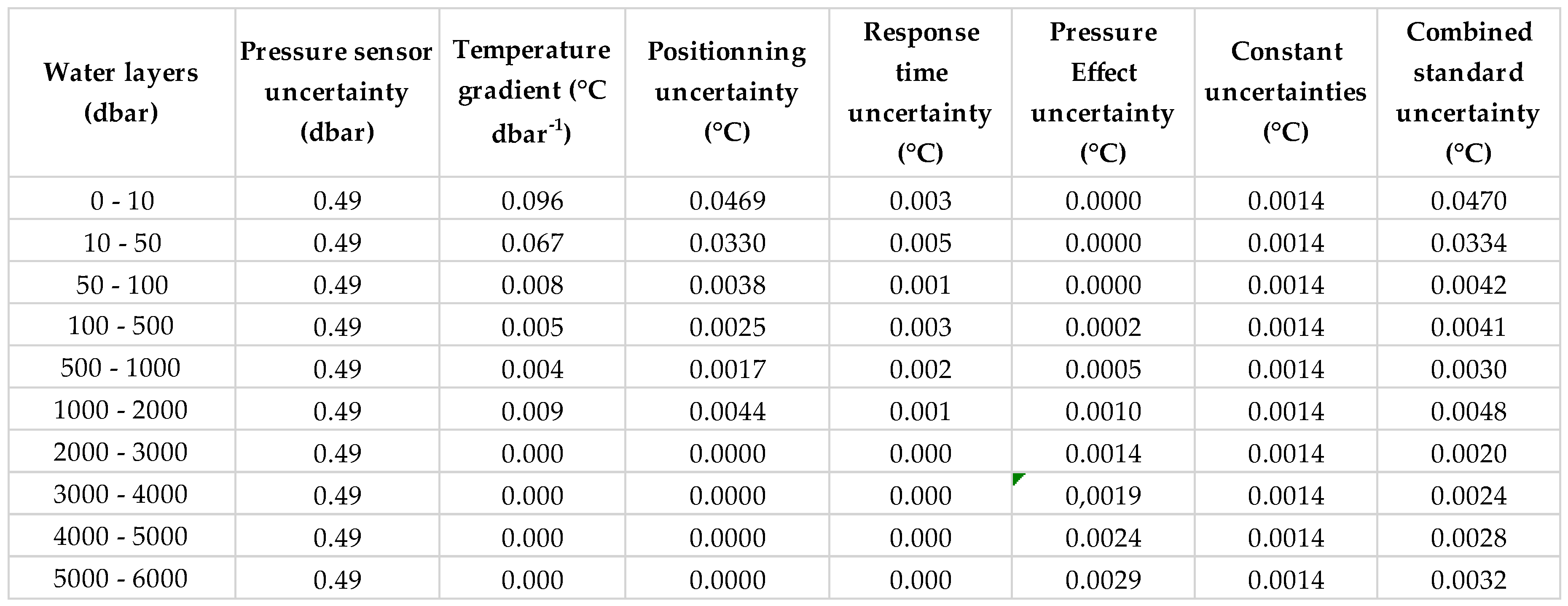
Table 3 gives values of response time uncertainties obtained from a CTD profile maid in the Mediterranean Sea on April 2024 (average longitude: 21.88, average latitude: 35.37), when the sea was quiet. The profile has been made to the depth of 2026 m. From 0 to 2000 dbar, the values of the response time uncertainty were obtained by using the product τ v. The Table is extrapolated to 600 bar to obtain values of the total standard uncertainty that takes into account the positioning and the pressure effect uncertainties. The column ‘Constant uncertainties’ makes the sum of uncertainties: linearity, self-heating, calibration, viscous heating and drift over time, given in the Table 2. It appears clearly that the response time uncertainty is not dominating the budget, even in the first layers.

5. Implementation of the Equations of the Measured Temperature

The relationship (10) was programmed under the Python software. As the carousel remains at a constant depth before the descents or the ascents, the initial sensor temperature is the same as the medium. The term

(T_{0} - T_{10})

is null.

In the relationship (8),

g r a d (T)

is the temperature difference between two depths given by the pressure sensor. The problem is to detect automatically slopes changes in the temperature record. This detection was made from the method described in [27]. This publication has given place to the Python package called Ruptures (http://ctruong.perso.math.cnrs.fr/ruptures), based on the combination of three factors: a cost function, a research method and a constraint. This package can be loaded at this address: https://github.com/deepcharles/ruptures. The cost function measures the number of breakpoints in the signal. The constraint corresponds to the number of breakpoints to detect. After trials and evaluations of different solutions, we used the cost function “Continuous Linear (CLinear)” that calculates the fitting error between the signal and a straight line. The research function we used is “Dynamic programming (Dynp)” that finds the minimum sum of costs by calculating the cost of all the sub-sequences of the signal under study. There can be a maximum of 29 breakpoints per descent and 29 per ascent corresponding to 60 gradients per profile. To avoid false detections due to the oscillating movements of the boat, the time between two detections is filtrated to 24 x 1/f, where 24 is the sampling frequency of the CTD profiler. A threshold is also applied to eliminate the quick temperature variations during the detection. The study of profiles acquired during a campaign, called GDG22 (see Section 7), made in the Bay of Biscay with a quiet sea, allowed to detect thermal gradients close to 1 °C dbar^-1. Another, carried out near the Faroe Islands (GN23) in very rough seas, found gradients of less than 0.3 °C dbar^-1. Therefore, thresholds have been fixed to 1 °C dbar^-1 for sea states ≤ 2 and 0.3 °C dbar^-1 for sea states > 2.

Relationships (6) and (10) require the calculation of v, the speed at which the cage rises or falls. v is obtained by calculating the ratio of the difference between two consecutive temperatures and the difference of time, from the original signal sampled at 24 Hz.

Relationships (10) and (11) require the determination of ω. ω is extracted from the pressure signal at the time when the carousel is in standby at the maximal depth for a few minutes. The boat oscillations are visible (see Figure 4 d)) and after using a low pass filter, a Fourier Transform (FT) can be applied. The positive frequencies of this FT are kept to calculate the power spectral density that allows to determine the principal frequency f of the signal.

Knowing the amplitude of oscillations is also required to calculate

Δ p (t, ω)

in the relationship (6). In standby phases, this amplitude depends essentially on the boat movements and on the lift of the carousel in the water. During descent and ascent phases, this is superimposed to the speed at which the cable unwinds. A sliding window FT is therefore required to measure this amplitude along the descent and ascent profiles, giving a spectrogram from which, we can extract the amplitude values at the frequency determined previously.

6. Results of the Implementation

Relationships (6) and (10) have been tested on a lot of profiles to fill a Table of results. To choose between these two relationships, the programme detects at first, the presence or absence of oscillations in the pressure signal when the profiler is at the bottom. As examples, the Figures 3 show the results of the application of the relationship (6) on a profile of 1500 m obtained in Mediterranean Sea with a quiet sea state of 2 and the Figures 4 show the application of the relation (10) on another one of 1000 m depth obtained in North Sea, selected because the ‘sea state’ was of a level 4. 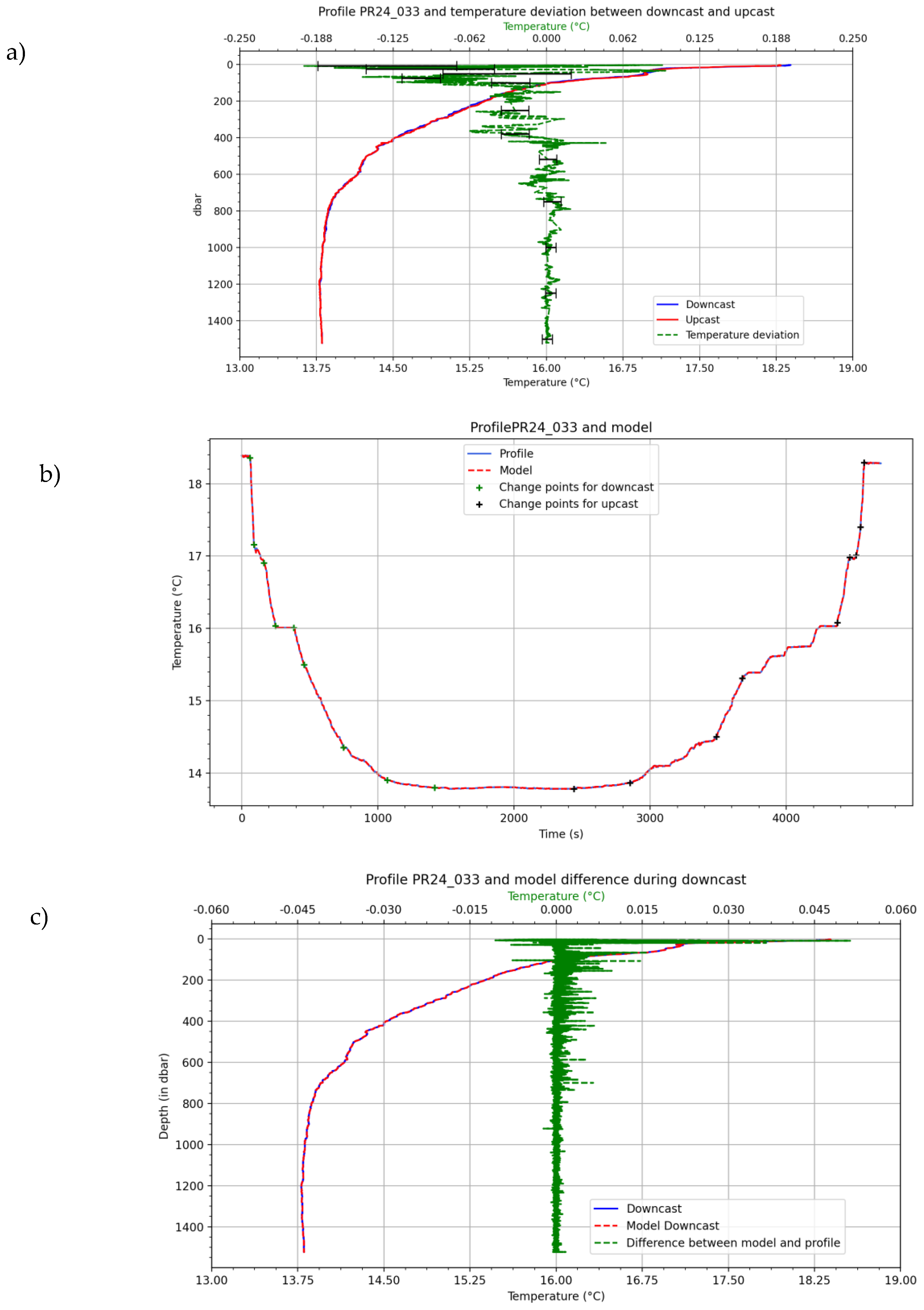Figure 3 a) shows the measured temperature during the downcast and the upcast and the error signal obtained from the two temperature sensors. This error signal

δ T

takes into account the difference in height of the two temperature sensors according to the relationship:

δ T = T_{b o t t o m} (p) - T_{t o p} (p - 1.4)

(12)

where T_bottom is the temperature measured by the sensor at the bottom of the carousel, T_top the temperature measured by the sensor located at the top and 1.4 the distance between the two sensors. The combined expanded uncertainty of

δ T

per water layer is superimposed on some values of the error signal located at 7, 24, 50, 75, 100, 225, 380, 500, 750, 1000, 1250 and 1500 dbar. It is obtained with Equation (2) multiplied by

2 \sqrt{2}

to take into account the two independent temperature values measured during the downcast and the upcast. The downcast lasted 32 min while the upcast lasted 45 min. At 0 m depth, the maximum delay is then 77 min and the maximal deviation is 0.198 °C. Down to a depth of about 700 m, the amplitude of the deviation signal is much greater than the instrumental uncertainty, demonstrating the natural variability of the medium between the moment of descent and the moment of ascent. Figure 3 b) shows the temperature profile as a function of time and the result of the numerical modelling of this signal obtained with the Equation (6). The two curves overlap perfectly. The 18 stars superimposed on the signal delimit the segments found by automatic slope change detection. Figure 3 c) shows the same results for the downcast temperature profile as a function of pressure, with added the signal of error between the model and the measured temperature. This error signal is significant in the first 10 m but its maximal amplitude is 0.05 °C so that the deviation signal of the Figure a) is between – 0.18 °C and + 0.08 °C. The origin of these errors can be partially attributed to the assumption that the term

(T_{0} - T_{10})

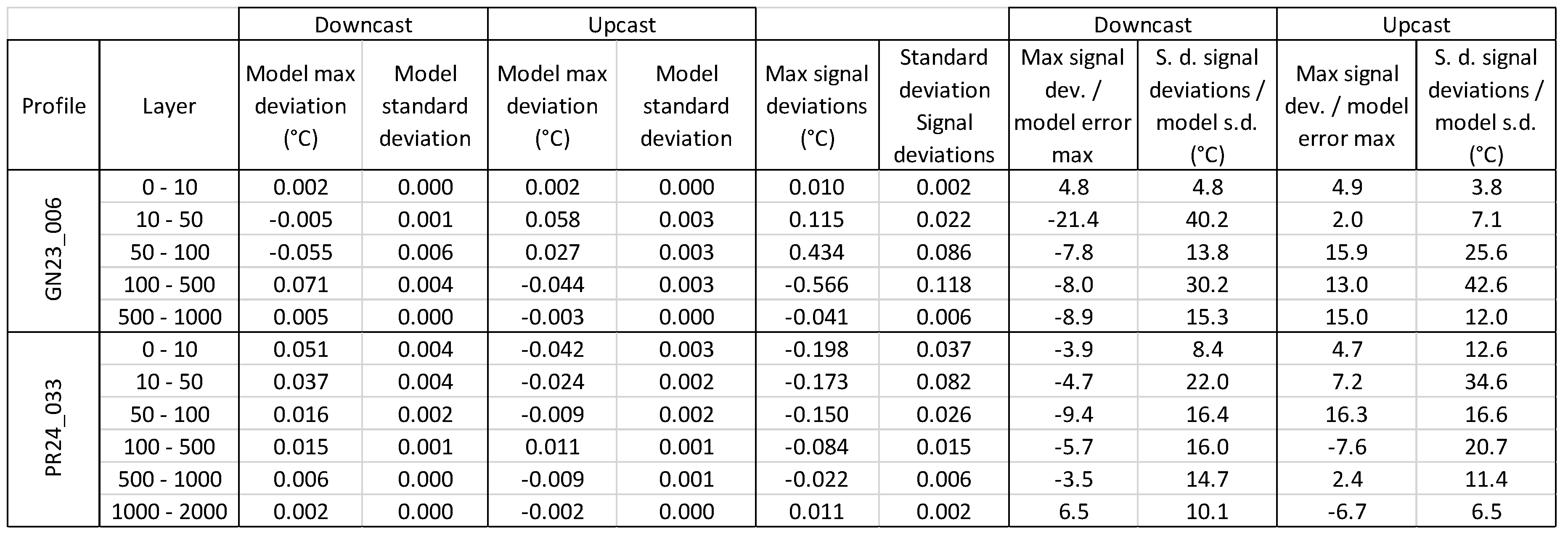
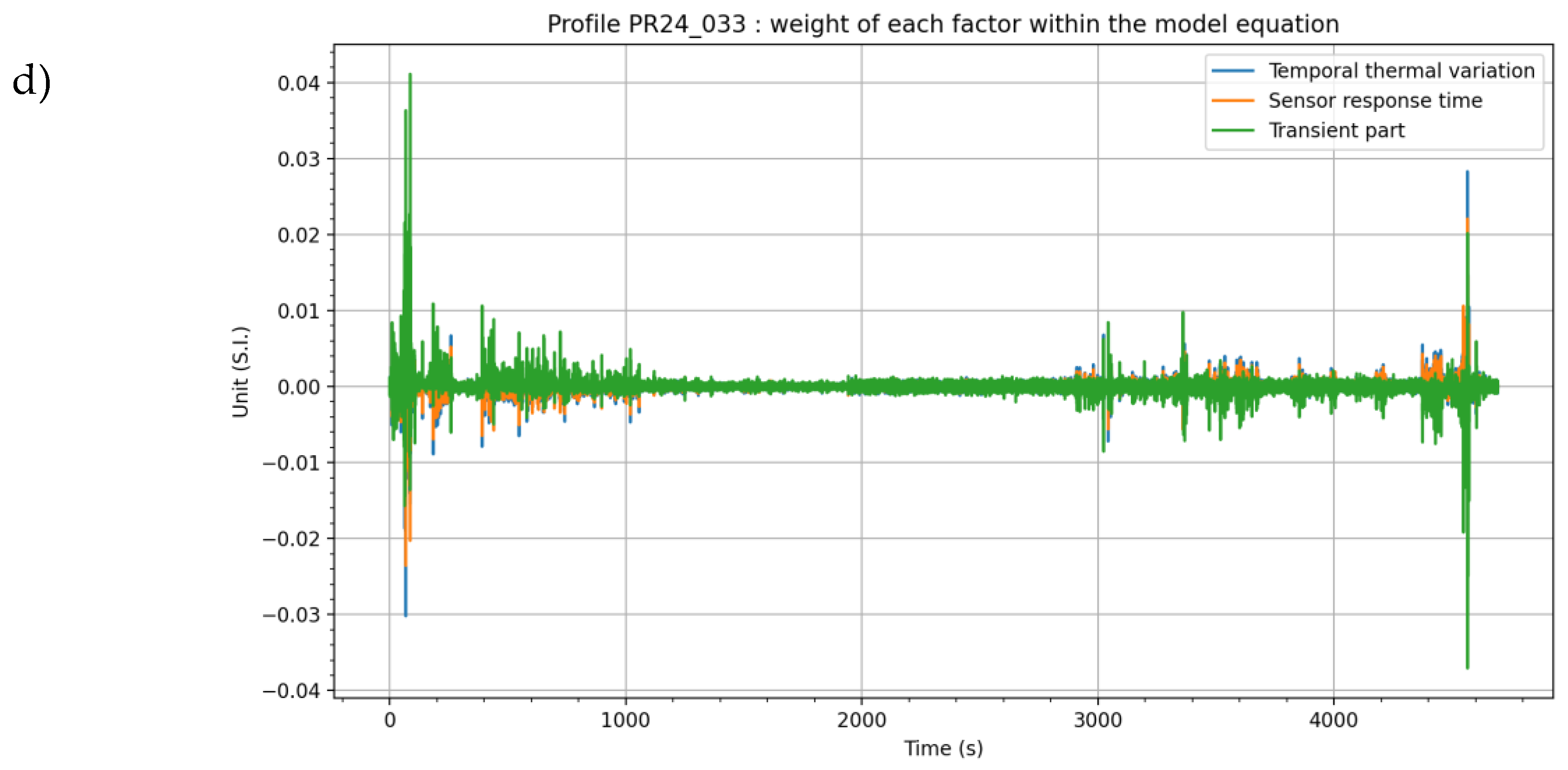
is null. This assumption is true at the beginning to the descent and at the beginning of the ascent, but not at the start of major temperature gradients. Table 4 gives the ratio values between these two signals per water layers. Finally, Figure 3 d) shows the amplitudes of the different terms of the Equation (6). The violet color represents the first part of Equation (6), i.e. the transient part of the sensor temperature rise. The red color represents the sensor’s response time error τv. The orange color represents the temporal thermal variations obtained with the vt term.

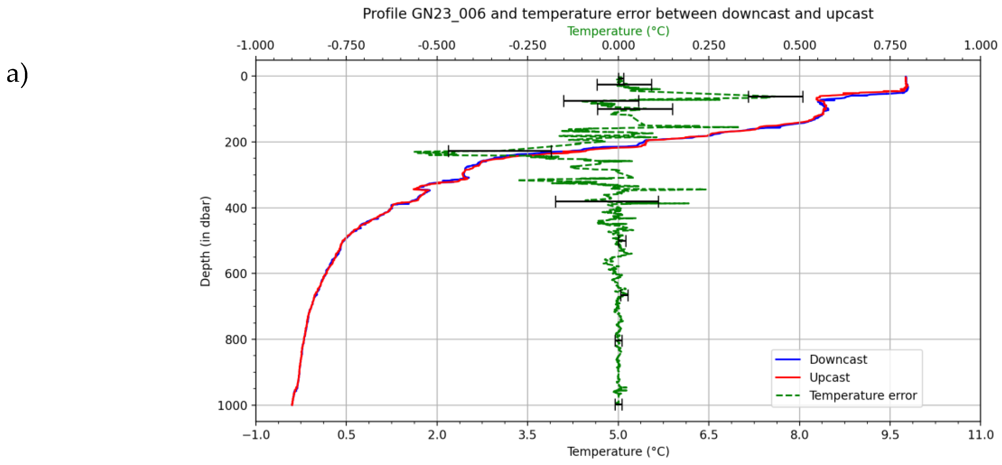
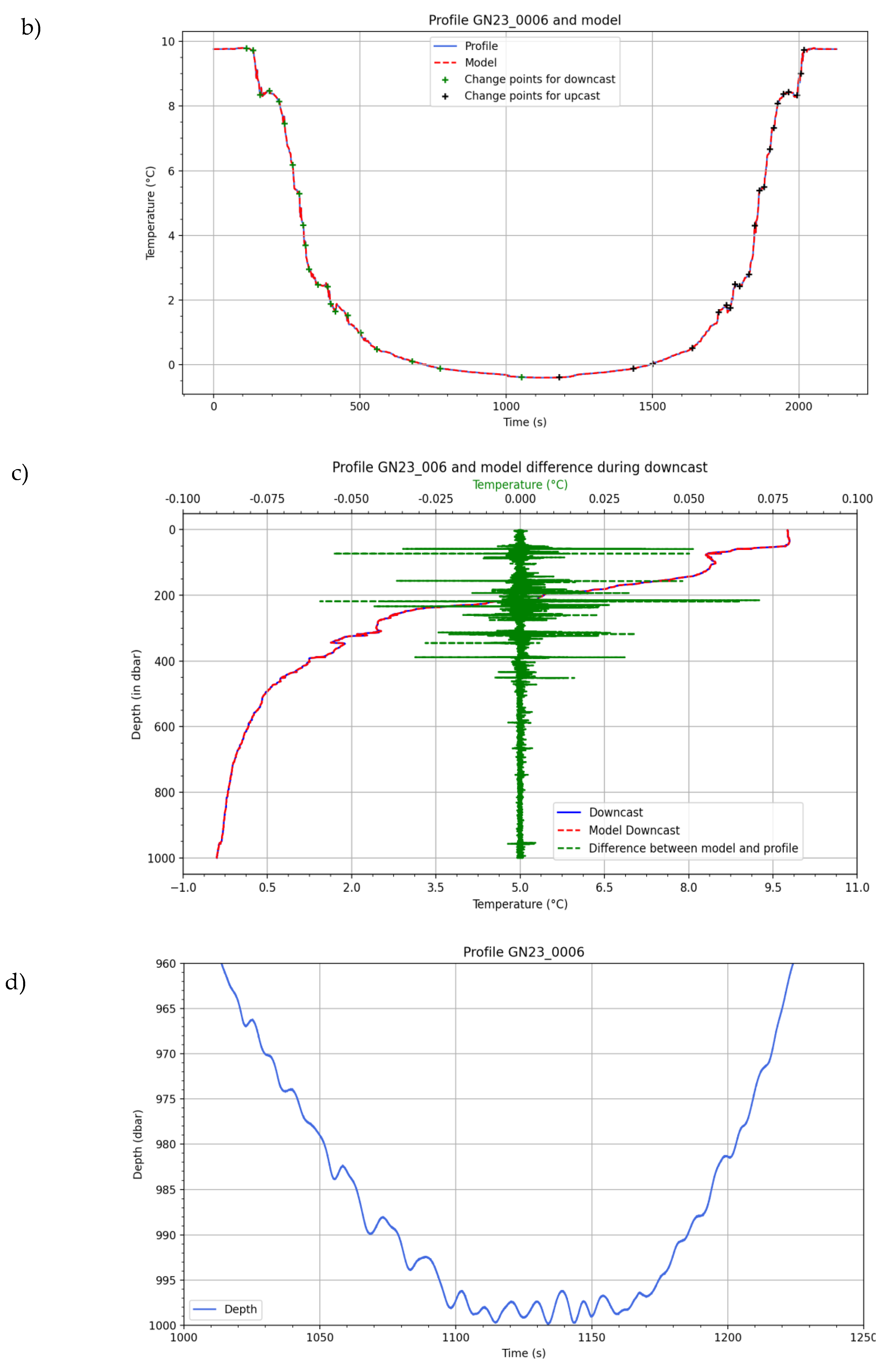
Figure 4a) shows also the measured temperature during the downcast and the upcast and the deviation signal calculated from the two temperature sensors but on a profile obtained with a sea state of 4. The downcast lasted 19 min and the upcast 16.5 min. At 0 m depth, the maximum delay is then 35.5 min and the maximal deviation is 0.01 °C in the layer 0 – 10 m. It should be noted that for this profile, the maximum deviation is in the 100 - 500 m range, and is therefore independent of the time between the measurement on descent and the measurement on ascent of the cage. The uncertainty bars are again smaller than the deviation signal in the first 400 metres. They are represented to the pressures 7, 24, 50, 75, 100, 225, 380, 500, 666, 804 and 998 dbar. Figure 4 b) shows the temperature profile as a function of time and the result of the numerical modelling of this signal obtained with Equation (10). One time again, the two curves overlap perfectly. 42 changes of slope were required to describe the gradients. Figure 4 c) shows the downcast temperature profile as a function of pressure with the numerical model superimposed, and in green the point by point errors between the model and the measured signal. It appears that the instantaneous errors are about ten times smaller than the spikes of the deviation signal of the Figure a), and probably in relation with the water mixing generated by the upward and downward movements of the carousel (see discussion in Section 8). Table 4 gives the ratio values between these two signals per water layers. Figure 4 d) shows the pressure signal with the time during which the cage is at rest before ascending. The oscillations associated with the movement of the boat are clearly visible. It is this part of the signal that is used to measure the pulsation ω of oscillations.

7. Location and Description of Measurement Sites Used

The data on which this study rely on were acquired in different environments regarding latitude, period of the year, oceanic processes. An overview of the dataset gathered for our purposes is given in Table 5 below.

The general comments about the data acquisition summed up in the Table 5 are the following :

-: all the profiles were acquired with the dual CT described previously.
-: All the data acquired during GdG22 are weakly influenced by large internal tides.
-: The only rather rough sea state conditions were met during the GN23 experiment and used as a reference to assess the influence of the rolling movement on the measured temperature model.
-: The most marked seasonal thermocline (~35 m / T 6 °C) where met during the GdG22 and is likely to experiment vertical oscillation of the order of 5 to 30 m amplitude (due to internal tide and internal solitary waves).
-: GIB20 and PR24 where performed in the vicinity of large mesoscale gyre (Alboran gyre) or eddies (Pelops anticyclone).

8. Discussion

Ship-based CTD profiles are used currently as reference to qualify temperature and salinity data from other instruments and in data assimilation with optimal estimation, but the uncertainties associated to these profiles are generally considered to be equivalent to the calibration uncertainties of the temperature or conductivity sensors of these instruments. The effect of the pressure measurements uncertainties are rarely considered, even though their contribution to the uncertainty budget of temperature measurements may be high, in particular in areas where the vertical temperature gradients are significant.

We could wonder if this problem is the same with ARGO profiling floats. As most drifting floats are fitted with Sea-Bird SBE 41 CTDs, it is possible to assess the uncertainties of their temperature measurements from the documents available on the Sea-Bird Scientific website. As the temperature sensor is identical to that of the CTD SBE 9+ profilers, its constant measurement uncertainties are identical to those given in Table 2, except for the drift over time u_d. In the Sea-Bird documentation, this is calculated at 0.2 mK/year instead of the measured 0.29 mK/year. If we take it into account over 4 years, the final uncertainty is 0.16 mK instead of 0.17 mK, but it does not change the final result.

Its response in temperature is given by the Equation (4). As the instrument ascends at a very low speed (≈ 0.1 m/s), the uncertainty linked to its response time during the crossing of temperature gradients will be smaller. For example, with a temperature gradient of 0.15 °C dbar^-1, its theoretical uncertainty is 0.001 °C so that for an SBE 9 at 1 m s^-1, the theoretical uncertainty is 0.010 °C.

Most of SBE 41 are equipped with the DRUCK PDCR 1830 pressure sensor [28]. The characteristics of this sensor can be retrieved from the Sea-Bird Scientific and DRUCK documents, and the pressure measurement standard combined uncertainty u_c(p_float) can be calculated thanks to Equation (13):

u_{c} (p_{f l o a t}) = \sqrt{{(\frac{u_{r}}{\sqrt{3}})}^{2} + {(\frac{u_{T s}}{\sqrt{6}})}^{2} + {(\frac{u_{d}}{\sqrt{3}})}^{2} + {(\frac{u_{h}}{\sqrt{3}})}^{2} + {(\frac{u_{c}}{\sqrt{6}})}^{2}}

(13)

Table 6 gives the results of this equation and the values of each term. The repeatability is taken from the document [28] Figure 3 (u_r = 0.25 dbar) and divided by the square root of 3 because 0.25 dbar is a maximum value. The lifetime drift (u_d = 1.5 dbar) is also taken from the Figure 1 of this document and divided by the square root of 3. The value of the hysteresis has not been found, but we can consider that it is included in the lifetime drift as the values of the Figure 1 come from measurements made when the floats were close to the surface after an ascent from 2000 m. The value of the thermal sensitivity can be found from DRUCK GE Sensing documents [29]. The temperature effect is of 0.3% of the full scale in the temperature error band and that gives u_Ts = 0.60 dbar. The uncertainty in relation with the calibration can be found in the datasheet SBE 41/41CP Argo CTD under the term of initial accuracy (u_c = ± 2 dbar). The thermal sensitivity and the initial accuracy have been divided by the square root of six, according to the paragraph F.2.3.3 of the reference [21]. The pressure combined standard uncertainty u_c(p_float) = 1.22 dbar, so that for an SBE 9+ it is 0.49 dbar. Argo floats do more accurate temperature measurements because of their low ascent speed makes that the error term τ v is very small, but they are clearly disadvantaged by the uncertainty budget of their pressure sensor when they meet temperature gradients. This is shown in Table 7, which uses the temperature gradient values from Table 3 up to 2000 m. In the layers 10 – 50 dbar and 50 – 100 dbar, the temperature combined standard uncertainty is multiplied by more than 2 compared to what is obtained with the SBE 911+.

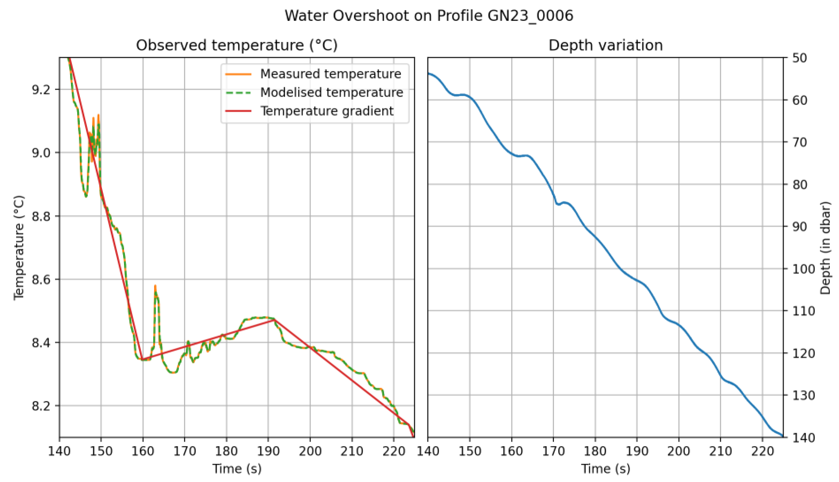
The other problem raised by this study concerns the large discrepancies observed in the first layers of water between the temperature measurements taken on descent and on ascent. These differences can be seen in graphs 3 a) and 4 a). They are generally much greater than the combined standard uncertainties calculated for the corresponding water layers. The Figure 5 is a zoom on one part of the profile GN23_006 of the Figure 4 b), between 140 and 230 s. We can see that rapid temperature variations of up to 0.26 °C are taken into account by the numerical model but they are not considered in the gradient’s detection. It is likely that with these oscillations, the carousel is dragged downwards then upwards (between 140 and 150 s) then upwards only (between 160 and 170 s) generating a mixing of the medium and large temperature measurement errors, compared with the gradients that should be measured. The sea state must therefore accounted for when processing temperature profiles, as it can lead to significant measurement errors, and in this case, it is difficult to distinguish the part of the measurement uncertainty linked to the natural variability of the environment and the part linked to the mixing of the medium by the carousel.

However, Figure 3 a) shows that when the sea is calm (sea state 2), in the first layers of water the differences in temperature between descent and ascent can also be significant compared with the calculated uncertainty. These differences can only be interpreted as the natural variability of the environment in the time between descent and ascent to a given depth. The uncertainty in the measurement of this variability can be estimated as the combined instrumental uncertainty calculated for each water Section.

In either case, this error signal can be interpreted as a measure of the representativeness of the CTD profile to within the combined instrumental uncertainties. However, these uncertainties may be greatly underestimated in gradients areas, in cases where the vessel is oscillating due to the sea state.

The results of four campaigns have been compiled in an Excel Table that contains:

-: the characteristics of the profile studied: coordinates, maximal depth, downcast duration, upcast duration;
-: the water layers such as those given in the first column of the Table 3;
-: the pressure measurement standard uncertainty corresponding to the uncertainty budget of Table 1;
-: the temperature maximal gradient per water layers, calculated with the Python programme;
-: the positioning uncertainty in depth, obtained by multiplying the two previous columns. As the maximum gradient is considered, the result is divided by the square root of 3;
-: the pressure effect uncertainty on the temperature sensor per water layer;
-: the temperature constant standard uncertainty of the temperature sensor as described in Table 3;
-: the maximal τ v values per water layer, found during the downcast and the upcast and divided by the square root of 3;
-: the uncertainty linked to the sensor response time and the boat movements. It corresponds to the difference between Equation (7) and the last term of Equation (10);
-: the expanded combined instrumental uncertainty calculated with the previous column, per water layers;
-: the maximum downward/upward error and the standard deviation of this error per water layer calculated with the relationship (12);
-: the amplitude of horizontal current component par water layer when available;
-: the presence or absence of internal waves.

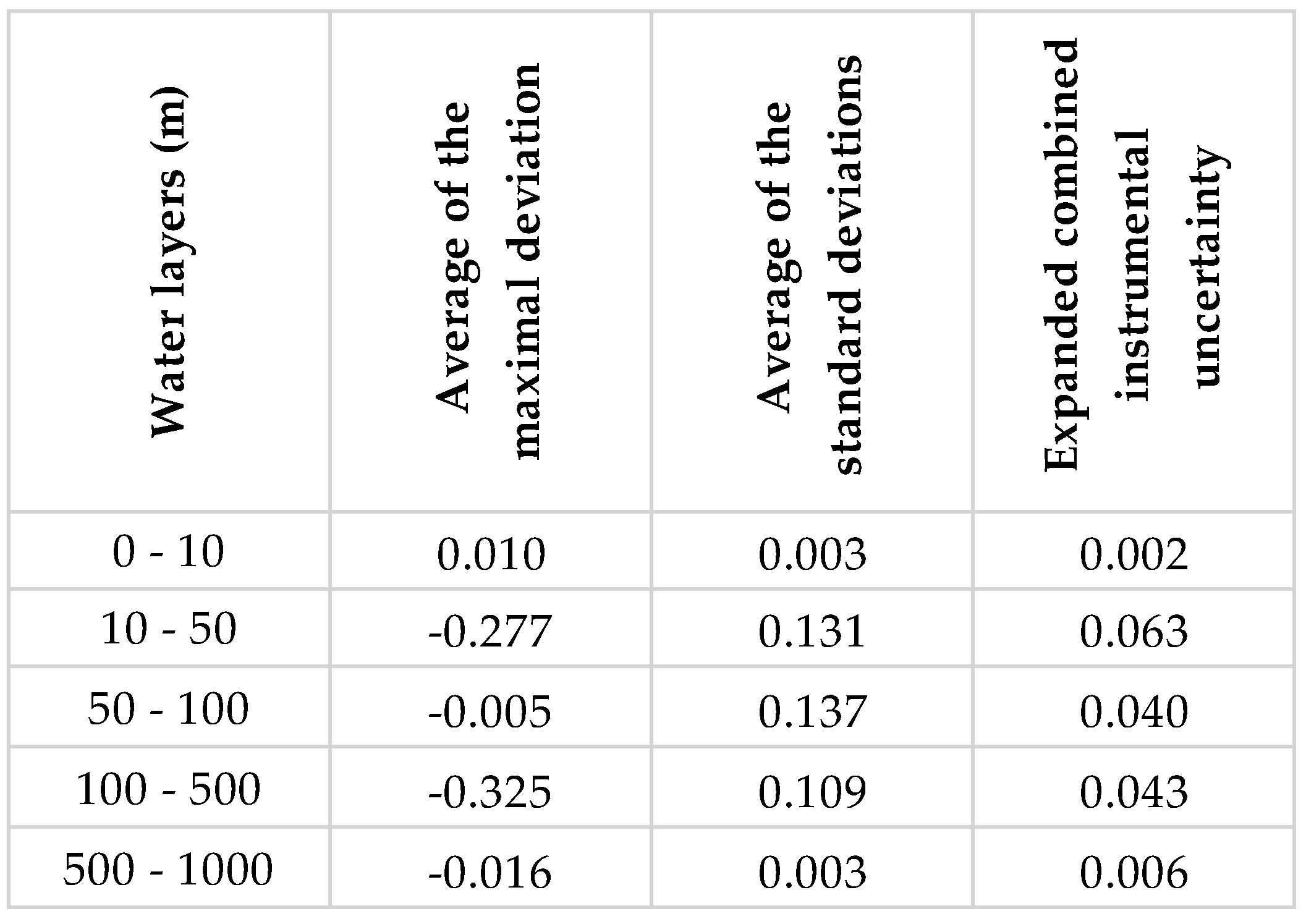
Table 8 gives an example of how to use the data of the Excel Table calculated from a campaign comprising six profiles carried out between 63.855 and 64.397 in latitude and 8.120 and 8.135 in longitude. The average durations of downcasts was of 13.5 ± 6 min and for upcasts 13.0 ± 8 min. It indicates the mean maximum deviation, the mean standard deviations and the expanded combined instrumental uncertainty (to 95 %), making it possible to quantify the representativeness of the data in this zone. It shows that, for this area, the RE defined in the introduction presents the same non-uniformity horizontally and vertically for depth between 10 and 500 m.

But, the ultimate aim of the Excel Table is to create a database that can be used to quantify the representativeness of CTD profiles carried out in areas close to the recorded profiles. Combined with a program based on artificial intelligence, it should make it possible to associate values of instrumental uncertainty and natural variability by water level, with profiles obtained with a single pair of sensors.

9. Conclusions

The dual-sensor CTD configuration is an innovation that allows the assessment of the representativeness of temperature profiles obtained during campaigns at sea. The work carried out on temperature profiles obtained using this method has shown that the representativeness of the profiles includes an instrumental uncertainty, but also a contribution of natural variability that is often much greater than the instrumental uncertainty in the first layers of water.

It has been possible to quantify the difference between the two by assessing the uncertainty of the measured temperature and establishing a model of the sensor's response to temperature variations. The factor that has the greatest influence on measurement uncertainty is the positioning of the temperature value as a function of pressure, in areas where pressure gradients are significant. So, while Argo floats do more accurate temperature measurements because of their low ascent speed, they are clearly disadvantaged by the uncertainty budget of their pressure sensor when they meet temperature gradients.

Another factor could be investigated to improve measurements in great depths (> 1100 m), it is the pressure sensitivity of SBE 3 sensors. A pressure characterisation of each sensor would be necessary to reduce this uncertainty to one and a half mK, as shown in the budget set out in Table 2.

The equation was used to calculate the uncertainty associated with the response time of the temperature sensor and to show that this uncertainty does not dominate the final result. It also shows that, the sea state must be taken into account when processing temperature profiles, as it can lead to significant measurement errors, and that in this case, it is difficult to distinguish the part of the measurement uncertainty linked to the natural variability of the environment and the part linked to the mixing of the medium by the carousel.

Author Contributions

Conceptualization, methodology, F. Dumas, writing—original draft preparation, writing—review and editing, M. Le Menn, F. Dumas; software, validation, B. Calvez. All authors have read and agreed to the published version of the manuscript. Please turn to the CRediT taxonomy for the term explanation.

Funding

this research is funded by Shom.

Conflicts of Interest

The authors declare no conflict of interest. The funders had no role in the design of the study; in the collection, analyses, or interpretation of data; in the writing of the manuscript, or in the decision to publish the results.

References

Saunders, P. M.; Mahrt, K-H.; Williams, R. T. Standard and Laboratory Calibration. WHP Operations and Methods, 1991.
Le Menn, M. About uncertainties in practical salinities calculations. Ocean Sci., 7, 651–659, 2011. [CrossRef]
Bordone, A. ; Pennecchi, F. ; Raiteri, G.; Repetti, L. and Reseghetti, F. XBT, ARGO Float and Ship-Based CTD Profiles Intercompared Under Strict Space-Time Conditions in the Mediterranean Sea: Assessment of Metrological Comparability. J. Mar. Sci. Eng., 8, 313, 2020. [CrossRef]
Gourion, J. and Szekely, T.; Killick, R.; Owens, B.; Reverdin, G.; Chapron, B. Improved Statistical Method for Quality Control of Hydrographic Observations. J. Atmos. Ocean. Technol., 37, 789-806, 2020. [CrossRef]
Gouretski, V.; Roquet, F. and Cheng, L. Measurement biases in ocean temperature profiles from marine mammal data loggers. J. Atmos. Ocean. Technol., 2024. [CrossRef]
Nappo, C.; Caneill, J.; Furman, R.; Gifford, F.; Kaimal, J.; Kramer, M.; et al. The workshop on the representativeness of meteorological observations. Bull. Am. Meteorol. Soc. 63, 761–764, 1981.
BIPM, JCGM 200:2012. International vocabulary of metrology – Basic and general concepts and associated terms (VIM). 3^rd edition, 2008 version with minor corrections.
Cowley, R.; Killick, R.E.; Boyer, T.; Gouretski, V.; Reseghetti, F.; Kizu, S.; Palmer, M.D.; Cheng, L.; Storto, A.; Le Menn, M.; Simoncelli, S.; Macdonald, A.M. and Domingues, C.M. International Quality-Controlled Ocean Database (IQuOD) v0.1: The Temperature Uncertainty Specification. Front. Mar. Sci. 8:689695, 2021. [CrossRef]
Daley, R. Atmospheric data analysis. Ed. Cambridge University Press, 1994.
Janji´c, T.; Bormann, N.; Bocquet, M.; Carton, J.A.; Cohn, S.E.; Dance, S.L.; Losa, S.N.; Nichols, N.K.; Potthast, R.; Waller, J.A.; Weston, P. On the representation error in data assimilation. Q. J. R. Meteorol Soc. 2018; 144:1257–1278. [CrossRef]
Sanikommu, S. ; Banerjee, D. S.; Baduru, B. et al. Impact of dynamical representational errors on an Indian Ocean ensemble data assimilation system. Q J R Meteorol Soc., 145: 3680–3691, 2019. [CrossRef]
Hodyss, D. and Nichols, N. The error of representation: basic understanding. Tellus A: Dynamic Meteorology and Oceanography, 67:1, 24822, 2015. [CrossRef]
Oke, P. R. and Sakov, P. Representation Error of Oceanic Observations for Data Assimilation. J. Atmos. Ocean. Technol, 25, 1004-1017, 2008. [CrossRef]
Zuo, H.; Balmaseda, M. A.; de Boisseson, E.; Hirahara, S.; Chrust, M.; de Rosnay, P. A generic ensemble generation scheme for data assimilation and ocean analysis. ECMWF Technical memorandum, 2017. https://www.ecmwf.int/sites/default/files/elibrary/2017/17831-generic-ensemble-generation-scheme-data-assimilation-and-ocean-analysis.pdf.
Schiller, A.; Oke, P.; Brassington, G.; Entel, M.; Fiedler, R.; Griffin, D. and Mansbridge, J. Eddy-resolving.
ocean circulation in the Asian-Australian region inferred from an ocean reanalysis effort. Progress in Oceanography, 76(3):334–365, 2008. ISSN 00796611. [CrossRef]
Rykova T. Improving forecasts of individual ocean eddies using feature mapping. Sci Rep. 2023 Apr 17;13(1):6216. PMID: 37069250; PMCID: PMC10110584. [CrossRef]
Sea-Bird Scientific. SBE 3F CTD temperature sensor datasheet, 2022. https://www.seabird.com/sbe-3f-3plus-3s-oceanographic-temperature-sensor/product-downloads?id=60762467708.
Uchida, H.; Ohyama, K.; Ozawa, S.; Fukasawa, M. In Situ Calibration of the SeaBird 9plus CTD Thermometer. J. Atmos. Ocean. Technol., 24, 2007. [CrossRef]
Uchida, H.; Nakano, T.; Tamba, J.; Widiatmo, J.V.; Yamazawa, K.; Ozawa, S.; Kawano, T. Deep ocean temperature measurement with an uncertainty of 0.7 mK. J. Atmos. Ocean. Technol., 32:2199-2210, 2015. doi.org/10.1175/JTECH-D-15-0013.1.
Peruzzi, A.; Ober, S.; Bosma, R. Effect of pressure on deep-ocean, thermometers, Int. J. Thermophys. 38, 163 2017. [CrossRef]
BIPM. Evaluation of measurement data – Guide to the expression of uncertainty in measurement. JCGM 100:2008, GUM 1995 with minor corrections, 2008.
Larson, N. and Pedersen A. M. Temperature measurements in flowing water: Viscous heating of sensor tips. Proc. First IGHEM Meeting, Montreal, QC, Canada, International Group for Hydraulic Efficiency Measurement, 1996. http://www.seabird.com/viscous-heating-sensor-tips.
Garreau, P.; Dumas, F.; Louazel, S.; Correard, S.; Fercocq, S.; Le Menn, M; Serpette, A .; Garnier, V.; Stegner, A.; Le Vu, B.; Doglioli, A. and Gregori, G. PROTEVS-MED field experiments: very high resolution hydrographic surveys in the Western Mediterranean Sea. Earth Syst. Sci. Data, 12, 441–456, 2020. [CrossRef]
Mensah, V.; Le Menn, M.; Morel, Y. Thermal Mass Correction for the Evaluation of Salinity, J. Atmos. Ocean. Technol., 26, 665-672, 2009. [CrossRef]
Le Menn, M. Instrumentation and Metrology in oceanography. ISTE – WILEY, 2012, pp.38-42. [CrossRef]
Le Menn, M.; Poli, P.; David, A.; Sagot, J.; Lucas, M.; O’Carroll, A.; Belbeoch, M. and Herklotz, K. Development of Surface Drifting Buoys for Fiducial Reference Measurements of Sea-Surface Temperature. Front. Mar. Sci. 6:578, 2019. [CrossRef]
Truong, C.; Oudre, L. et Vayatis, N. Selective review of offline change point detection methods. Signal Processing, 167, 2020. [CrossRef]
Sea-Bird Scientific. Comparison of Argo float pressure sensor performance: Druck versus Kistler. February 2015. https://www.seabird.com/sbe-41-argo-ctd/product-downloads?id=54627907875.
GE Sensing. 1830/1840 Series, Druck High Performance Level Pressure Sensors. https://www.trescal.com/wp-content/uploads/sites/85/2023/09/ptx1830.pdf.

Figure 1. Carousel water sampler used for the measurements at sea. The SBE 9⁺ CTD profiler is located at the bottom with the first pair of CT sensors. The second pair (not visible on this photo) is located at the top. The pump and the pipe connecting it to the conductivity sensor are visible in the foreground.

Figure 2. Drift over time of SBE 3 sensors used during the campaigns at sea.

Figure 3. a) Measured temperature during the downcast and the upcast and the deviation signal obtained from the two temperature sensors. The combined expanded uncertainty per water layer is superimposed to the error signal (black bars). b) temperature profile as a function of time and result of the numerical modelling of this signal obtained with Equation (6). The stars show the segments detected by the automated detection of slope changes. c) downcast temperature profile as a function of pressure with the overlapped numerical model and in green, the error signal between the model and the measurement. d) Amplitudes of the different terms of the Equation (6). The green color represents the transient part of the sensor temperature rise of equation. The orange color represents the sensor’s response time error τ v. The blue color represents the temporal thermal variations obtained with the v t term.

Figure 4. a) Measured temperature during the downcast and the upcast and the deviation signal obtained from the two temperature sensors. The total expanded uncertainty per water layer is superimposed to the deviation signal (black bars). b) temperature profile as a function of time and result of the numerical modelling of this signal obtained with Equation (10). The stars show the segments detected by the automated detection of slope changes. c) downcast temperature profile as a function of pressure with the overlapped numerical model and the instantaneous errors between the model and the measured signal. d) Zoom of the pressure signal between the descent phase and the ascent phase to illustrate the oscillations due to the movement of the boat.

Figure 5. On the left, enlargement of one part of the descent of profile no. 0006 (orange line) and visualisation of the numerical model obtained with Equation (8) (green line). Large and rapid variations in temperature appear that doesn’t follow the detected temperature gradients (in red). On the right, visualisation of the corresponding recorded pressure variations.

Table 1. Uncertainty budget of the SBE 9+ sn 766 pressure sensor calculated from Equation (1), in the case of the double sensor configuration.

Table 2. Temperature uncertainty budget obtained from Equation (2), at the surface and at 600 bar for an SBE 3 probe which pressure effect on the sensor has not been measured and compensated.

Table 3. Calculation of the combined standard uncertainty with values taken from a profile (PR24_026 0 – 2026 dbar) obtained in the Mediterranean Sea on April 2024. The calculations are extrapolated to 6000 dbar with values close to real of temperature gradients, to see the influence of the pressure effect uncertainties and of the pressure positioning uncertainties on the total uncertainty at 600 bar.

Table 4. Show the maximum and the standard deviation of the model vs the measured signal per water layer. The same parameters are given for the deviation signal (downcast – upcast), and the ratio between the deviation signal and the model is calculated. The maximal errors of the model are between 2 and 21.4 times smaller than the deviation signal, and the standard deviations of the model are between 3.8 and 42.6 times smaller than the deviation signal.

Table 5. Summary of the campaigns used in this study.

Table 6. Standard combined uncertainty of the DRUCK PDCR 1830 pressure sensor installed on the CTD SBE 41 of ARGO floats, calculated with Equation (13).

Table 7. Uncertainty budget of an Argo float calculated from the temperature gradients of the Table 3 (profile PR24_026, 0 – 2026 dbar obtained in the Mediterranean Sea on April 2024 with a CTD SBE 911+).

Table 8. Example of how to quantify the representativeness of data per water layers, for a campaign comprising six profiles located between 63.855 and 64.397 in latitude and 8.120 and 8.135 in longitude and of average duration 26.5 ± 7 min

Disclaimer/Publisher’s Note: The statements, opinions and data contained in all publications are solely those of the individual author(s) and contributor(s) and not of MDPI and/or the editor(s). MDPI and/or the editor(s) disclaim responsibility for any injury to people or property resulting from any ideas, methods, instructions or products referred to in the content.

© 2024 by the authors. Licensee MDPI, Basel, Switzerland. This article is an open access article distributed under the terms and conditions of the Creative Commons Attribution (CC BY) license (http://creativecommons.org/licenses/by/4.0/).

Copyright: This open access article is published under a Creative Commons CC BY 4.0 license, which permit the free download, distribution, and reuse, provided that the author and preprint are cited in any reuse.

MDPI Initiatives

Important Links

Choose an area of interest and we will send you notifications of new preprints at your preferred frequency.

Disclaimer

Assessment of the Representativeness and Uncertainties of CTD Temperature Profiles

Abstract

1. Introduction

2. The Experimental Apparatus

3. The Measurements Uncertainties of Temperature Measurements

4. The Equation of the Measured Temperature

5. Implementation of the Equations of the Measured Temperature

6. Results of the Implementation

7. Location and Description of Measurement Sites Used

8. Discussion

9. Conclusions

Author Contributions

Funding

Conflicts of Interest

References

MDPI Initiatives

Important Links

Subscribe