Submitted:
11 December 2024
Posted:
12 December 2024
You are already at the latest version
Abstract
This study examines the effectiveness of generalised additive models (GAMs) and log-log linear models for estimating the parameters of the generalised extreme value (GEV) distribution, which are then used to estimate flood quantiles in ungauged catchments. This is known as parameter regression technique (PRT). Using data from 88 gauged catchments in New South Wales, Australia, flood quantiles corresponding to various Annual Exceedance Probabilities (AEP) were estimated, which were then used as dependent variables and several catchment characteristics were used as independent variables. GAMs were employed to capture non-linearities in flood generation processes. The study evaluates different GAM and log-log linear models, identifying the best ones based on significant predictors and various statistical metrics using a leave one out (LOO) validation approach. Results indicate that GAMs provide more accurate and reliable predictions of flood quantiles compared to the log-log linear models, demonstrating better performance in capturing observed values across different quantiles. The absolute median relative error percentage (REr%) ranges from 33% to 39% for the GAMs, and from 36% to 45% for the log-log models. GAM demonstrates better performance compared to log-log linear models for quantiles Q2, Q5, Q10, Q20, and Q50; however, their performance appears to be similar for Q100.
Keywords:
Floods
; GAM
; Rainfall
; regional flood frequency
; quantile regression
; parameter
1. Introduction
In recent years, there has been a significant acceleration in climate change, accompanied by a noticeable increase in the frequency of extreme weather events, even in regions that historically experienced lower occurrences [1,2]. While flooding is a natural phenomenon, human involvements, such as the alteration of natural watercourses, changes in land use, and the influence of climate change, can modify how watersheds respond to rainfall, leading to extreme floods [3,4]. To evaluate flood risks, statistical methods are employed to analyse long-term streamflow data and estimate flood magnitudes for specific return periods or annual exceedance probabilities (AEP). Moreover, more intense rainfall increases the risk of damaging floods, especially in urban areas lacking infrastructure resilience. Recent trends worldwide, including Australia, Europe, the United States, Canada, and China, clearly show an increasing occurrence of severe floods [5,6]. This highlights the need for accurate flood quantile predictions to design and manage infrastructure such as urban drainage systems, spillways, bridges, and levees to reduce flood damage. Consequently, flood frequency analysis (FFA) is a widely used method for design flood estimation, relying on sufficient recorded streamflow data at specific locations. However, many stream-gauging sites have limited or short-term flow data, and numerous streams remain ungauged. To address this challenge in ungauged catchments, regional flood frequency analysis (RFFA) is commonly employed [7,8].
While log-linear regression models are often used in RFFA, sometimes simple log transformations may not capture the complexities and non-linearities present in flood generation processes [15]. Flood processes often show non-linear behaviour that linear models or simple transformations cannot sufficiently capture, necessitating the use of more complex modelling approaches like Generalised Additive Models (GAMs) to account for these complexities [9].
GAMs have gained popularity in various fields, including hydrology, due to their effectiveness in modelling complex relationships between variables. They offer flexibility in capturing non-linear relationships without requiring restrictive assumptions and have been widely adopted for analysing hydrological data [10,11]. In hydrology, GAMs have shown promise in estimating non-linear trends in water quality, predicting temperature, evaluating air quality pollutants, and more. They outperform multiple linear regression models due to their incorporation of smooth functions, effectively handling complex relationships between predictor and dependent variables [12]. GAMs have been employed in recent studies on RFFA. For instance, Singh et al. [13] used Generalised Additive Models for Location Scale and Shape (GAMLSS) parameters in Canada to capture both linear and non-linear characteristics of flood peak changes. Similarly, Wang et al. [14] examined summer precipitation data from 21 rainfall stations in China using GAMLSS. Additionally, Chen et al. [3] applied GAMLSS to implement time-varying non-stationary flood frequency analysis and precipitation-informed models across 161 catchments in the UK. Furthermore, Souaissi et al. [7] employed GAMs in regional frequency analysis of stream temperature at 24 stations in Switzerland.
Some studies have recognised the ability of GAM in RFFA. For example, Noor et al. [15] compared the performance of GAM in RFFA with Quantile Regression Technique (QRT) using 114 catchments in Victoria, Australia. The findings suggest that while GAMs demonstrate superior performance for smaller return periods, QRT outperforms GAM for higher return periods. Ouarda et al. [16] introduced GAMs for estimating low-flow characteristics in ungauged stations in Quebec, Canada at a regional scale and compared them to multiple linear regression. Results indicated that GAMs demonstrate superior performance compared to multiple linear regression in estimating low-flow characteristics. Furthermore, Rahman et al. [17] compared various RFFA methods, including GAM with fixed regions, log-linear models, canonical correlation analysis, and the region-of-influence approach, using data from 85 gauged catchments in New South Wales (NSW), Australia. Through a leave-one-out validation approach (LOO), GAM methods generally surpassed the others. Chebana et al. [9] evaluated both linear and non-linear approaches, indicating that RFFA models based on GAMs demonstrated better performance compared to linear models, including the commonly used log-linear regression model, using a dataset consisting of 151 stations in Quebec, Canada. Qu et al. [11] compared the analysis of linear and non-linear quantile regression models and demonstrated superior performance of the GAM for location, scale, and shape parameters particularly in estimating design flood values, suggesting its feasibility for practical applications.
Australian hydrology shows high variability, suggesting that the linearity assumption may not be suitable for developing RFFA models in Australia. In this context, GAMs offer a better means to handle non-linearity in regression models. However, there have been relatively few studies on the application of GAMs in RFFA in Australia. Previous GAMs related RFFA research in Australia primarily focused on QRT, with limited exploration within the parameter regression technique (PRT) framework. For example, Rahman et al. [17] compared the performance of GAM-based RFFA models with log-linear model and canonical correlation analysis for estimating two flood quantiles (Q10 and Q50) in Australian conditions. In another study, Noor et al. [15] applied GAMs in RFFA to 114 catchments in Victoria, Australia, and compared their performances with the QRT. In both Rahman et al [17] and Noor et al. [15], log-Pearson Type 3 (LP3) distribution was adopted to estimate at-site flood quantiles which were used the dependent variables in their analysis. In contrast, this study applies GAMs in the PRT framework using Generalised Extreme Value (GEV) distribution (i.e., prediction equations are developed for the three parameters of the GEV distribution) and compares their performance with traditional log-log linear regression models. By focusing on PRT in RFFA, this study fills a knowledge gap in the application of GAMs within RFFA. To the authors knowledge, there is no RFFA study where GAMs are applied to regionalise the parameters of the GEV distribution. The remainder of this paper is structured as follows: Section 2 introduces the study area and data used in this study; Section 3 outlines the methodology employed in this study, while the results are discussed in Section 4. Following the results, section 5 provides a discussion, and section 6 contains conclusions of the study.
Study Area and Data
In this research, 88 gauged catchments were selected from the state of NSW, Australia. These catchments are of smaller to medium sizes, making them well-suited for RFFA. The selected catchments vary in size, with areas ranging from 8 to 1010 km2. The average catchment size is 325 km2, with a median size of 260 km2. The record lengths of annual maximum floods (AMF) vary from 25 to 89 years, with an average record length of 48 years and a median of 44 years. The location of these selected catchments is presented in Figure 1.
Eight catchment characteristics were selected in this study. Table 1 summarises the catchment characteristics data, presenting the minimum, maximum, mean, and standard deviation values for each of the following characteristics.
Catchment Area (Area): This is an important predictor variable in RFFA and the main scaling factor. It has been adopted in all the previous RFFA studies.
Design Rainfall Intensity (I6,2): Rainfall intensity plays a crucial role in flood generation. It is essential for estimating flood magnitudes for specific durations and annual exceedance probabilities (AEP). In this study, a duration of six hours and return period of 2 years is selected as the mean critical duration of the selected catchments.
Mean Annual Rainfall (MAR): Although it does not directly impact flood peak generation, it serves as a proxy for other variables affecting runoff, such as evapotranspiration, catchment wetness and land use.
Shape Factor (SF): This parameter assesses the influence of catchment shape on the runoff hydrograph peak.
Mean Annual Evapotranspiration (MAE): Evapotranspiration, which combines evaporation and transpiration, affects water availability for runoff and recharge processes.
Stream Density (SDEN): SDEN quantifies the potential for runoff, with higher values indicating efficient drainage mechanisms and a greater potential for runoff peak, which can contribute to flooding.
Slope factor (S1085): The S1085 index represents mainstream channel slope, affecting flood speed. High values mean steep slopes, leading to faster floods and riskier floods in flood zones.
Forest coverage (FOREST): This parameter can significantly influence hydrological processes by affecting infiltration rates and runoff within catchments.
Methodology
For the estimation of flood quantiles corresponding to AEP of 1 in 2, 5, 10, 20, 50, and 100 years (denoted respectively as Q2, Q5, Q10, Q20, Q50 and Q100), this study used the GEV distribution with L-moments fitting method. The GEV parameters including location (represented by the mean), scale (coefficient of variation (LCV) from L-moments), and shape (coefficient of skewness (LSK) from L-moments, equivalent to shape for GEV), were considered as dependent variables. These parameters were estimated by PRT using two statistical methods, GAM and log-log multiple linear regression. Additionally, the study used the eight catchment characteristics described above as predictor variables in modelling.
Generalised Extreme Value Distribution
This study adopts a GEV distribution coupled with L-moments as suggested by Hosking and Wallis [18]. The L-moments are similar to the conventional moments; however, they have several theoretical advantages, e.g., being able to model a wider range of distributions and when estimated from a sample they tend to be more robust to the presence of outliers in the dataset [18].
The GEV distribution, introduced by Jenkinson [19], is given by:
Where ξ, α, and κ are the location, scale, and shape parameters, respectively. The shape parameter κ defines the tail behaviour of the distribution. If κ < 0 (Frechet), the distribution has a heavy right-hand tail and a lower bound equal to ξ + α/κ; if κ > 0 (Weibull), the distribution has an upper bound of ξ + α/κ; and when κ = 0, the GEV distribution reduces to the Gumbel distribution whose cdf is given by
and has an exponential upper tail.
The T-year event (where T is a surrogate for ARI) can be expressed in terms of the GEV parameters.
The L-Moment estimators for the parameters of the GEV distribution are:
where the expression for the shape parameter
is an approximation provided by Hosking et al. [20]
that is accurate for –0.5 < < 0.5. is the LSK estimator, and = b0, = 2b1 – b0, and = 6b2 – 6b1 + b0 are the L- moments estimators of the mean, scale and skew. Here, br is taken to be the unbiased estimators of the first three probability weighted moments (PWM).
yT =-ln[-ln(1-1/T)] is the Gumbel reduced variate; = regional LCV (estimated as discussed below); and = shape parameter of GEV distribution; to estimate this, (regional LSK) is to be estimated first, as explained below.
Generalised Additive Model (GAM)
GAM is a statistical approach that incorporates non-linear functions for each variable while maintaining the model's additive nature. Mathematically, a GAM can be expressed as follows:
Where is the response variable, is a constant term, represents non-linear functions for each predictor variable and is the error term.
In this equation, g(μi) represents the link function applied to the expected value (mean) of the response variable for the i-th observation, often denoted as E(Yᵢ); Xᵢ is a vector of predictor variables for the i-th observation; b is a vector of coefficients associated with the predictor variables; and ∑ⱼ indicates a summation over the predictor variables, with fj(xᵢⱼ) representing the non-linear functions (often smooth functions) applied to each predictor variable xᵢⱼ for the i-th observation.
Log-Log linear
Log-log is a linear relationship between the predictor variables (X) and the response variable (Y). The model can be represented as:
Where Y is the response variable (e.g. mean, LCV and LSK); are the predictor variable (e.g. catchments characteristics); are the coefficients to be estimated; and represents the error term.
Evaluation Statistics
Model validation involves assessing each developed model using a leave-one-out (LOO) validation procedure as described by Haddad et al. [22]. To compare the model's performance, several evaluation statistics are used, including the median ratio of predicted to observed quantiles, the absolute median relative error (Median REr) expressed as a percentage, the mean squared error (MSE), the relative root mean square error (rRMSE) expressed as a percentage, the mean bias (BIAS), and the relative mean bias (rBIAS) expressed as a percentage. The equations for these evaluation statistics are as follows:
where Qobs is obtained by at-site FFA fitting a GEV distribution to the AMF data, and Qpred is obtained by RFFA technique, adopted in this study.
Results
Estimation of GEV Distribution Parameters:
Table 2 presents the GEV parameters estimated for 88 catchments using L-moments method with FLIKE software. The GEV parameters, including mean, LCV, and LSK, are provided along with their minimum, maximum, mean, and standard deviation values. GAM and Log-Log linear models were employed to estimate the parameters of the GEV distribution. The analysis was conducted separately for the mean, LCV, and LSK parameters.
The approach involved extensive exploration of all possible combinations of the eight predictor variables, resulting in a total of 255 models. Evaluation criteria included R2, Generalised Cross-Validation (GCV) score, and model complexity.
Following a comprehensive assessment, a subset of models showing promising performance in explanatory power and simplicity was identified. Subsequent validation through LOO cross-validation confirmed the reliability of selected models and highlighted those with strong predictive variables. Final model selection selected those retaining significant predictors while achieving high R2 values, low GCV scores, low degree of freedom for residuals (df residual), minimised Akaike Information Criterion (AIC) values and Bayesian Information Criterion (BIC). This approach ensured the selection of models having an effective balance between predictive accuracy and complexity, providing a strong analytical framework.
Generalised Additive Models (GAMs)
Mean Parameter Estimation
For the estimation of the C was based on R2, GCV scores, and model complexity. Among the 255 models, eight were considered and after performing LOO validation, the significant predictor variables for each model were identified based on p-value (0.05 significance level) as shown in Table 3.
Interestingly, Model 3 and Model 6 revealed significance in all their predictor variables, highlighting their strong relationship with the mean parameter. For Model 3, the parametric coefficients were estimated, with both 'area' and 'I62' demonstrating significant effects on the mean. From Table 4, the R2 value was 0.60, indicating that 60% of the variance in the mean was explained. The GCV score was 2208814.13. The analysis revealed that both 'area' and 'I62' had statistically significant relationships with the mean parameter.
Model 6 indicated that 'area', 'I62', and 'MAE' were all significant predictors of the mean parameter. From Table 4, the R2 value increased to 0.70, indicating that the model explained 70% of the variance in the mean. The GCV score decreased to 483878.03. The analysis highlighted the combined influence of 'area', 'I62', and 'MAE' in predicting the mean parameter.
Among all the models, Model 6 appears to be the best choice, as it has the highest R2 value, the lowest GCV score, a lower AIC, and a lower value for df residual. However, Model 3 is less complex. Both Model 6 and Model 3 are taken into consideration in building the models.
LCV Parameter Estimation
Similarly, various models were assessed for their ability to estimate LCV while considering model complexity, goodness-of-fit metrics, and significance of predictor variables. The best eight different GAMs were chosen to estimate LCV using various predictor variables. After performing LOO validation, the significant predictor variables for each model were determined based on p-values (0.05 significance level). The models, along with their significant predictor variables, are summarised in Table 5. Notably, Model 3 and Model 8 revealed significance in all their predictor variables, indicating a strong relationship with the LCV variable.
To evaluate the performance of these models, several metrics were considered, including AIC and df residual and goodness-of-fit statistics such as R2 and GCV scores (as shown in Table 6). Model 3 appears to be the most suitable choice for estimating LCV, with a good R2 value (0.53), a low GCV score (0.16), a low AIC (-184.08), and a low value for residual (70.41). This indicates that Model 3 provides the best balance between goodness of fit and model complexity. On the other hand, Model 8 offers a good option due to its simplicity with an R2 of 0.17 and a GCV score of 4.36. Both models 3 and 8 are taken in consideration in building the models.
LSK Parameter Estimation
Likewise, different models were evaluated in terms of their ability to predict LSK, taking into account the same factors such as model complexity, metrics indicating goodness of fit, and the importance of predictor variables. Eight distinct GAMs were developed to predict LSK, incorporating a variety of predictor variables. The summary in Table 7 outlines the models and highlights their significant predictor variables.
After LOO validation, the models were compared based on their R2 values, GCV, AIC and df residual as shown in Table 8.
Among the models, Model 7 stands out as the most promising with a R2 value of 0.33, signifying that approximately 33% of the variability in LSK is explained by the model. Moreover, the GCV score for Model 7 was notably lower than that of other alternatives, indicating its effectiveness in minimising overfitting. Additionally, the model had a lower AIC and a reduced df residual. Overall, Model 7 demonstrated a significant impact of I62 and SF on LSK prediction. Both terms are statistically significant based on their p-values. On the other hand, Model 8, while less complex, still explains 17% of the deviance with a focus on I62. Both model 7 and 8 are taken in consideration in building the models.
Evaluation of GAM Model Combinations for Quantile Prediction
To explore the effectiveness of GAM analysis in quantile prediction, eight distinct combinations, denoted as GAM (a) through GAM (h), are assessed to determine their predictive capabilities. Each combination comprises specific models for Mean, LCV and LSK. They are as follow:
GAM (a): Mean (model 3) – LCV (model 8) – LSK (model 7)
GAM (b): Mean (model 3) – LCV (model 8) – LSK (model 8)
GAM (c): Mean (model 3) – LCV (model 3) – LSK (model 7)
GAM (d): Mean (model 3) – LCV (model 3) – LSK (model 8)
GAM (e): Mean (model 6) – LCV (model 8) – LSK (model 7)
GAM (f): Mean (model 6) – LCV (model 8) – LSK (model 8)
GAM (g): Mean (model 6) – LCV (model 3) – LSK (model 7)
GAM (h): Mean (model 6) – LCV (model 3) – LSK (model 8)
To determine the best combinations among the GAM models, the median of the ratio of observed to predicted values (Qobs/Qpred) and the median REr% for each combination were compared. As shown in Table 9, for the median ratio, combinations e, f, g, and h demonstrated median ratios close to 1, suggesting a good balance between observed and predicted values. Conversely, combinations a, b, c, and d had median ratios slightly higher than 1, indicating slightly overestimated predictions. Regarding the median REr%, combinations e, f, g, and h exhibited the lowest values across all quantiles, indicating the lowest percentage of relative errors. In contrast, combinations a, b, c, and d had higher median REr% values, indicating higher relative errors in prediction. Overall, combinations e, f, g, and h performed better than combinations a, b, c, and d in terms of both median ratio and median REr%.
Log-Log Linear:
Mean Parameter Estimation
For the estimation of the mean parameter using log-log linear, nine models were evaluated to determine the best predictor variables. After conducting LOO validation, these models (presented in Table 10) were assessed based on their significant predictor variables and overall performance.
The best models, based on the significant predictor variables and less complexity, were models 3 and 4. Model 3 included the predictor variables log(area) and log(I62), while model 4 incorporated log(area), log(I62), and log(SF) as significant predictors. From Table 11, Model 3 showed a R2 value of 0.75, indicating a good fit and demonstrating that the selected predictor variables explained a significant proportion of the variance in the mean parameter. Model 4 exhibited a slightly higher R2 value of 0.76, suggesting that the addition of log(SF) as a predictor improved the model's performance. It also had a lower AIC and BIC, indicating strong explanatory power.
Overall, models 3 and 4 will be taken into consideration in building the log-log models.
LCV Parameter Estimation
In this section, log-log linear models were employed to estimate the LCV parameter. Nine models were evaluated to determine the best predictor variables for LCV. After conducting LOO validation, nine models (presented in Table 12) were assessed based on their significant predictor variables and overall performance.
From Table 13, Model 8, which used "log(I62)" as the only predictor variable, showed an R2 value of 0.09. While Model 8's R2 value is relatively low, it was the best-performing model among the options available. This model is characterised by simplicity with a single predictor variable, "log(I62)" and therefore, it is the most suitable choice for estimating LCV using the log-log linear approach.
LSK Parameter Estimation
In this section, log-log linear models were used to estimate the LSK parameter. Nine models were assessed to determine the best predictor variables for LSK. After conducting LOO validation, these models were evaluated based on their significant predictor variables and overall performance (see Table 14).
While Model 8's adjusted R2 value is relatively low (as shown in Table 15), it was the best-performing model among the available options. Same as LCV, model 8 is the most suitable choice for estimating LSK using log-log linear due to its simplicity and relationship.
Evaluation of log-log Model Combinations for Quantile Prediction:
To investigate the effectiveness of log-log analysis in quantiles prediction, two specific combinations, denoted as log-log (i) and log-log (j) were examined for estimating quantiles using the Mean (from Model 3 and 4), LCV (from Model 8), and LSK (from Model 8) parameters. The combinations are as below:
Log – log (i): Mean (Model 3) – LCV (Model 8) – LSK (Model 8)
Log – log (j): Mean (Model 4) – LCV (Model 8) – LSK (Model 8)
For log-log (i), the median REr, expressed as percentage, ranges from 38.92% to 45.19% and the MSE ranges from y 4493.74 to 259758.43 across different quantiles. While for log-log (j), the median REr ranges from approximately 36.32% to 38.84% with the MSE ranging from approximately 4930.74 to 265092.08 across different quantiles. Figure 2 shows that the median REr and MSE for both models are relatively close to each other across different quantiles. This suggests that both combinations are effective in estimating quantiles using the Mean, LCV, and LSK parameters.
Comparison between GAM and Log-Log:
In summary, both GAMs and log-log linear models showed promising results for estimating different parameters (mean, LCV, and LSK). The choice between them depends on factors like model complexity, goodness of fit, and specific data characteristics.
Table 16 presents a comparison between GAM and log-log models, focusing on median REr% across the six quantiles Q2 to Q100. The median REr% ranges from 33% to 39% for GAM and from 35% to 45% for log-log models. Analysis of the minimum error reveals that, except for Q100, GAM generally exhibits lower median REr% compared to log-log, suggesting a better performance in most cases. Similarly, considering the maximum error, GAM demonstrates lower median REr% across all quantiles except for Q100, giving better predictive accuracy. Notably, for quantiles Q2, Q5, Q10, Q20, and Q50, GAM outperforms log-log model, while for Q100, their performance is very similar.
The boxplots, shown in Figure 3 and 4, illustrates the ratio (Qpred/Qobs) for the selected combinations of models. For combinations e, f, g, and h, representing GAM models, the median values for all the AEPs closely align with the 1:1 line, indicating a strong match between predicted and observed flood quantiles. Similarly, for combinations i and j, corresponding to log-log linear models, the median values are slightly above the 1:1 line, suggesting a generally good estimation of flood quantiles compared to observed values. Consistent lower quartile values across all the combinations indicates similar performance in the lower range of the ratio values for both GAM and log-log linear models. However, the upper quartile values for GAM models are lower than those for the log-log linear models, indicating lower variability in the overestimation of flood quantiles for GAM models. Moreover, except for AEPs of 1 in 2 and 100 years, the upper whisker values for GAM models are smaller than those for log-log linear models, suggesting that while maximum overestimation may be higher for the log-log models, the variability range is wider compared to GAM models. Conversely, the lower whisker values for GAM models are larger than those for log-log linear models, indicating higher minimum overestimation for GAM models but less variability in underestimation for log-log linear models.
In conclusion, the boxplot analysis suggests that GAM models, particularly combinations e, f, g, and h, exhibit slightly better performance in estimating flood quantiles compared to the log-log linear models (combinations i and j). The close alignment of median ratio values with the 1:1 line, coupled with lower variability in overestimation, highlights the effectiveness of GAM models in accurately predicting flood magnitudes across different quantiles.
The boxplots, presented in Figure 5 and Figure 6, reveal the distribution of the relative error % across the different combinations of models. For combinations e, f, g, and h, which represent GAM models, the median lines for all AEPs closely track with the 1:1 line, indicating a consistent pattern in error distribution. Similarly, for combinations i and j, corresponding to log-log linear models, the median lines for the relative error % values are near the 1:1 line, suggesting overall accuracy in error estimation. Consistent lower quartile values across all the combinations indicate similar performance in the lower range of relative error % values for both GAM and log-log linear models. However, the upper quartile values for GAM models are lower than those for log-log linear models, indicating less variability in the overestimation of errors for GAM models. Additionally, except for AEPs of 1 in 2 and 100 years, the upper whisker values for GAM models are smaller than those for log-log linear models, suggesting a thinner range of maximum overestimation for GAM models. Conversely, the lower whisker values for GAM models are larger than those for log-log linear models, indicating higher minimum overestimation for GAM models but less variability in underestimation for log-log linear models. Overall, the analysis of relative error % suggests that GAM models exhibit consistent error patterns across different AEPs, with less variability in overestimation compared to the log-log linear models.
Figure 7 illustrates the comparison between median ratio and median REr% for both GAM and log-log linear models. For the GAM models (e, f, g, h) the median ratio values are generally close to 1 across all the quantiles, except for Q100, indicating a good balance between observed and predicted values. In contrast, the log-log linear models (i, j) show median ratio values slightly above or below 1, suggesting some deviation between observed and predicted values. Therefore, GAM models provide more accurate and precise predictions compared to the log-log linear models, as indicated by the closer alignment of median ratio values to 1. Moreover, the GAM models demonstrate a better ability to capture the variability in flood magnitudes, as evidenced by their lower median REr% values across most quantiles. Conversely, the log-log linear models generally generate higher median REr% values, indicating relatively larger errors in prediction.
Overall, the findings suggest that the GAM models provide more reliable and accurate predictions of flood quantiles compared to the log-log linear models. The closer alignment of median ratio values to 1 for GAM models underscores their superior performance in capturing observed values across the different quantiles, highlighting their potential for enhancing flood prediction accuracy.
Table 17 presents the rBIAS and rRMSE percentages for different quantiles of the GAM (e, f, g, h) and log-log linear (i, j) models. For rBIAS (%), negative values indicate a tendency for underestimation, while positive values indicate overestimation. Among the GAM models (e, f, g, h), rBIAS values are consistently negative across all the quantiles, indicating a tendency for underestimation. Conversely, rBIAS values for the log-log linear models (i, j) are consistently positive, indicating a tendency for overestimation. Overall, the GAM models exhibit lowest bias values compared to the log-log linear models.
Regarding rRMSE (%), lower values indicate better model performance. Across all the quantiles, rRMSE values for the GAM models are generally lower compared to the log-log linear models. rRMSE values range from 56% to 63% for GAM and from 57% to 65% for log-log. This suggests that the GAM models have lower relative root mean square errors, indicating better performance in terms of accuracy and precision
Our results indicate that the GAM models (e, f, g, h) outperform the log-log linear models (i, j) in terms of bias and rRMSE across various quantiles, suggesting better accuracy and precision in predicting flood quantiles. Overall, based on the comparison of median ratio and median REr%, the GAM models (e, f, g, h) appear to outperform the log-log linear models (i, j) in terms of accuracy and precision in predicting flood quantiles.
Discussion
Our study reveals that GAMs show better performance compared to the log-log models for quantiles corresponding to return periods of 2 to 50 years, with consistently lower median REr% ranging from 33% to 39%. However, for higher return periods, log-log models sometimes demonstrate similar performance, with median REr% ranging from 36% to 45%. This finding suggests that the choice between GAMs and log-log models may rely on the specific return period of interest, and the selection of the predictor variables, with GAMs being more effective than the log-log models.
In comparison to previous research studies, our results align with Ali and Rahman [23], who reported median REr% values of 28–36% for 2 to 10 years return periods in southeast Australia using kriging-based RFFA techniques. Similarly, Zalnezhad et al. [24] found median REr% values ranging from 38% to 60% in the same region employing artificial neural networks (ANN) based RFFA technique. Aziz et al. [25] documented median REr values in the range of 35-44% using ANN in eastern Australia. Additionally, Noor et al. [15] found that GAM provides more accurate quantile estimates than QRT for smaller return periods, while QRT outperforms GAM for higher return periods, with median REr% values for 2, 5, and 10 years return periods ranging from 16% to 41% in Victoria.
Furthermore, Rahman et al. [26] reported median REr% in the range of 33% to 44% for the QRT model and 48% to 59% for the PRT model for design flood estimation in NSW, which is comparable to the relative error values (57% to 64%) reported for the RFFA technique recommended in the Australian Rainfall and Runoff [27]. Chebana et al. [9] also noted that models using GAM outperform those using log-linear regression as well as other methods applied to their dataset. Moreover, Ouarda et al. [16] found that the use of GAMs instead of the linear model significantly enhances performance.
Conclusion
This study compares the performance of PRT using GAM and log-log linear models to predict flood quantiles in ungauged catchments. Using data from 88 gauged catchments in NSW, Australia, the analysis was conducted for estimating parameters of the GEV distribution with the L-moment fitting method, separately for the mean, LCV, and LSK parameters. Flood quantiles corresponding to various AEP ranging from 1 in 2 to 1 in 100 years were estimated. Eight catchment characteristics, including catchment area, design rainfall intensity, mean annual rainfall, shape factor, mean annual evapotranspiration, stream density, slope factor, and forest coverage, were employed as predictor variables. The analysis involved a careful selection process among 255 models for each prediction technique, considering factors such as R2 values, GCV scores (for GAM modelling), and model complexity. Promising models were identified based on their performance in explanatory power and simplicity, validated through LOO cross-validation.
GAM, designed to capture non-linearities in flood processes, outperform log-log linear models across most quantiles exhibiting lower median REr% values and demonstrating better ability to capture flood magnitude variability. However, their effectiveness appears sometimes to be nearly comparable for Q100.
This outcome underscores the effectiveness of GAM models in predicting flood magnitudes across different quantiles, highlighting their potential for enhancing flood prediction accuracy. Comparing GAM and log-log models provides valuable insights into the factors affecting the accuracy of flood quantile estimation. This helps in choosing the right modelling techniques for different ranges of return periods, which may vary based on the specific return period and the selection of predictor variables.
Given how important it is to accurately predict floods for managing risks and planning infrastructure, this study suggests using GAMs with PRT in flood frequency analysis, especially in ungauged catchments where data is limited. However, it also identifies the need for further research and validation studies to explore the robustness and applicability of both modelling approaches across diverse hydrological settings and regions. Future research may include investigating the impacts of climate change on RFFA, exploring uncertainty analysis techniques, and extending the application of GAM-based approaches to larger geographic regions to further refine flood quantile estimation models.
Author Contributions
Data analysis and manuscript drafting: L.R.; conceptualisation,editing and supervision: A.R., conceptualisation, investigation, editing and supervision: K.H.
Funding
This research received no funding.
Institutional Review Board Statement
Not applicable.
Informed Consent Statement
Not applicable.
Data Availability Statement
The data used in this study can be obtained from Australian Government authorities by paying a prescribed fee.
Acknowledgments
Authors would like to acknowledge Australian Rainfall and Runoff Revision Project 5 team for providing some of the data. TUFLOW FLIKE was provided freely by Flike sales team. Streamflow data were obtained from WaterNSW.
Conflicts of Interest
The authors declare no conflict of interest.
References
- Hartmann, D. L. , Tank, A. M. K., Rusticucci, M., Alexander, L. V., Brönnimann, S., Charabi, Y. A. R.,... & Zhai, P. (2013). Observations: atmosphere and surface. In Climate change 2013 the physical science basis: Working group I contribution to the fifth assessment report of the intergovernmental panel on climate change (pp. 159-254). Cambridge University Press.
- Sheffield, J. , & Wood, E. F. (2012). Drought: past problems and future scenarios. Routledge.
- Chen, M., Papadikis, K., Jun, C., & Macdonald, N. (2023). Linear, nonlinear, parametric and nonparametric regression models for nonstationary flood frequency analysis. Journal of Hydrology, 616, 128772.
- Tellman, B. , Sullivan, J. A., Kuhn, C., Kettner, A. J., Doyle, C. S., Brakenridge, G. R.,... & Slayback, D. A. (2021). Satellite imaging reveals increased proportion of population exposed to floods. Nature, 596(7870), 80-86.
- Buttle, J. M. , Allen, D. M., Caissie, D., Davison, B., Hayashi, M., Peters, D. L.,... & Whitfield, P. H. (2016). Flood processes in Canada: Regional and special aspects. Canadian Water Resources Journal/Revue canadienne des ressources hydriques, 41(1-2), 7-30.
- Villarini, G., Smith, J. A., Serinaldi, F., Bales, J., Bates, P. D., & Krajewski, W. F. (2009). Flood frequency analysis for nonstationary annual peak records in an urban drainage basin. Advances in water resources, 32(8), 1255-1266.
- Souaissi, Z. , Ouarda, T. B., St-Hilaire, A., & Ouali, D. (2023). Regional frequency analysis of stream temperature at ungauged sites using non-linear canonical correlation analysis and generalized additive models. Environmental Modelling & Software, 163, 105682.
- Micevski, T. , Hackelbusch, A., Haddad, K., Kuczera, G., & Rahman, A. (2015). Regionalisation of the parameters of the log-Pearson 3 distribution: A case study for New South Wales, Australia. Hydrological Processes, 29(2), 250-260.
- Chebana, F., Charron, C., Ouarda, T. B., & Martel, B. (2014). Regional frequency analysis at ungauged sites with the generalized additive model. Journal of Hydrometeorology, 15(6), 2418-2428.
- Li, J., Lei, Y., Tan, S., Bell, C. D., Engel, B. A., & Wang, Y. (2018). Nonstationary flood frequency analysis for annual flood peak and volume series in both univariate and bivariate domain. Water resources management, 32, 4239-4252.
- Qu, C. , Li, J., Yan, L., Yan, P., Cheng, F., & Lu, D. (2020). Non-stationary flood frequency analysis using cubic B-spline-based GAMLSS model. Water, 12(7), 1867.
- Rahman, A., Charron, C., Ouarda, T. B., & Chebana, F. (2018). Development of regional flood frequency analysis techniques using generalized additive models for Australia. Stochastic environmental research and risk assessment, 32, 123-139.
- Singh, J., Ghosh, S., Simonovic, S. P., & Karmakar, S. (2021). Identification of flood seasonality and drivers across Canada. Hydrological Processes, 35(10), e14398.
- Wang, Y. , Li, J., Feng, P., & Hu, R. (2015). A time-dependent drought index for non-stationary precipitation series. Water Resources Management, 29, 5631-5647.
- Noor, F. , Laz, O. U., Haddad, K., Alim, M. A., & Rahman, A. (2022). Comparison between Quantile Regression Technique and Generalised Additive Model for Regional Flood Frequency Analysis: A Case Study for Victoria, Australia. Water, 14(22), 3627.
- Ouarda, T. B. , Charron, C., Hundecha, Y., St-Hilaire, A., & Chebana, F. (2018). Introduction of the GAM model for regional low-flow frequency analysis at ungauged basins and comparison with commonly used approaches. Environmental modelling & software, 109, 256-271.
- Rahman, A., Charron, C., Ouarda, T. B., & Chebana, F. (2018). Development of regional flood frequency analysis techniques using generalized additive models for Australia. Stochastic environmental research and risk assessment, 32, 123-139.
- Hosking, J. R. M. , & Wallis, J. R. (1997). Regional frequency analysis (p. 240).
- Jenkinson, A. F. (1955). The frequency distribution of the annual maximum (or minimum) values of meteorological elements. Quarterly Journal of the Royal meteorological society, 81(348), 158-171.
- Hosking, J. R. M. , Wallis, J. R., & Wood, E. F. (1985). Estimation of the generalized extreme-value distribution by the method of probability-weighted moments. Technometrics, 27(3), 251-261.
- Madsen, H. , Pearson, C. P., & Rosbjerg, D. (1997). Comparison of annual maximum series and partial duration series methods for modeling extreme hydrologic events: 2. Regional modeling. Water Resources Research, 33(4), 759-769.
- Haddad, K., Rahman, A., Zaman, M. A., & Shrestha, S. (2013). Applicability of Monte Carlo cross validation technique for model development and validation using generalised least squares regression. Journal of Hydrology, 482, 119-128.
- Ali, S.; Rahman, A. Development of a Kriging Based Regional Flood Frequency Analysis Technique for South-East Australia, Natural Hazards. 2022. Available online: https://link.springer.com/article/10.1007/s11069-022-05488-4 (accessed on 6 November 2022).
- Zalnezhad, A.; Rahman, A.; Nasiri, N.; Vafakhah, M.; Samali, B.; Ahamed, F. Comparing Performance of ANN and SVM Methods for Regional Flood Frequency Analysis in South-East Australia. Water 2022, 14, 3323.Insurance Council of Australia (ICA). (2022, May 3). Updated data shows 2022 flood was Australia’s costliest. Available online: https://insurancecouncil.com.au/wp-content/uploads/2022/05/220503-East-Coast-flood-event-costs-update.pdf.
- Aziz, K. , Rahman, A., Fang, G., & Shrestha, S. (2014). Application of artificial neural networks in regional flood frequency analysis: a case study for Australia. Stochastic environmental research and risk assessment, 28, 541-554.
- Rahman, A. S., Khan, Z., & Rahman, A. (2020). Application of independent component analysis in regional flood frequency analysis: Comparison between quantile regression and parameter regression techniques. Journal of Hydrology, 581, 124372.
- Rahman, A. , Haddad, K., Kuczera, G., & Weinmann, E. (2019). Regional flood methods. Australian Rainfall and Runoff: A Guide to Flood Estimation. Book 3, Peak Flow Estimation, 105-146.
Figure 1.
Location of study catchments in NSW, Australia.
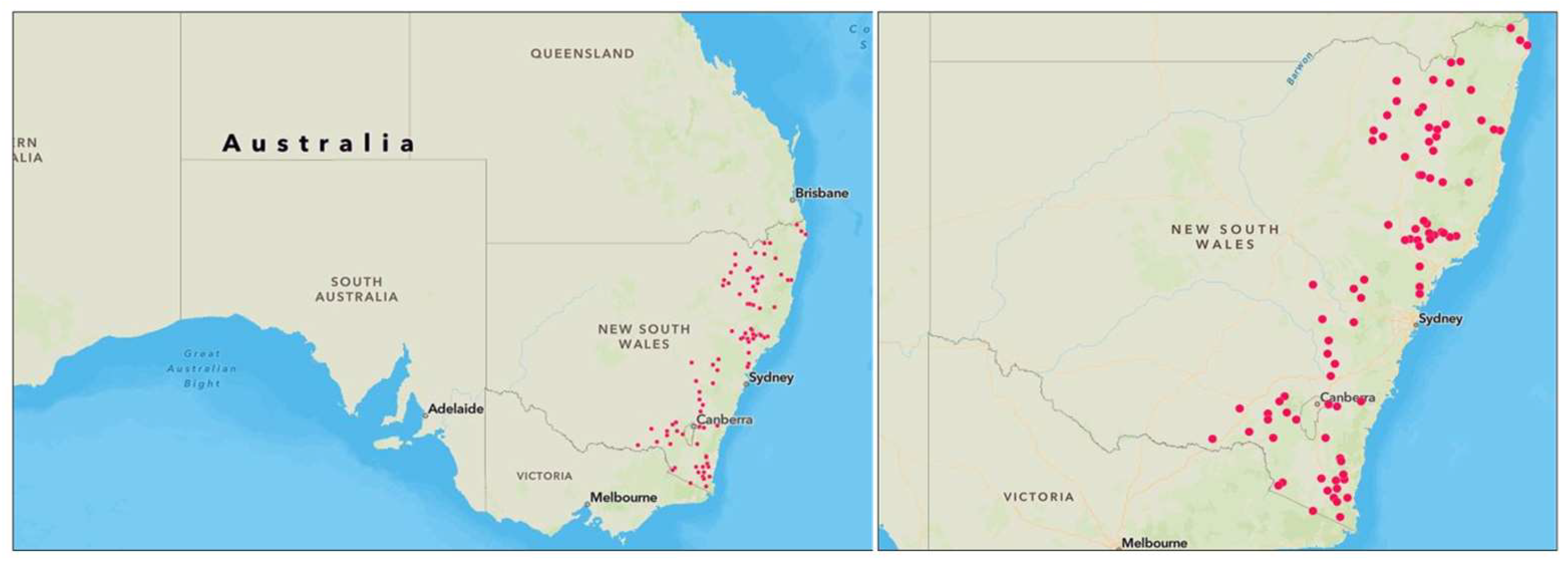
Figure 2.
Median REr% and MSE for the selected log-log Combinations.
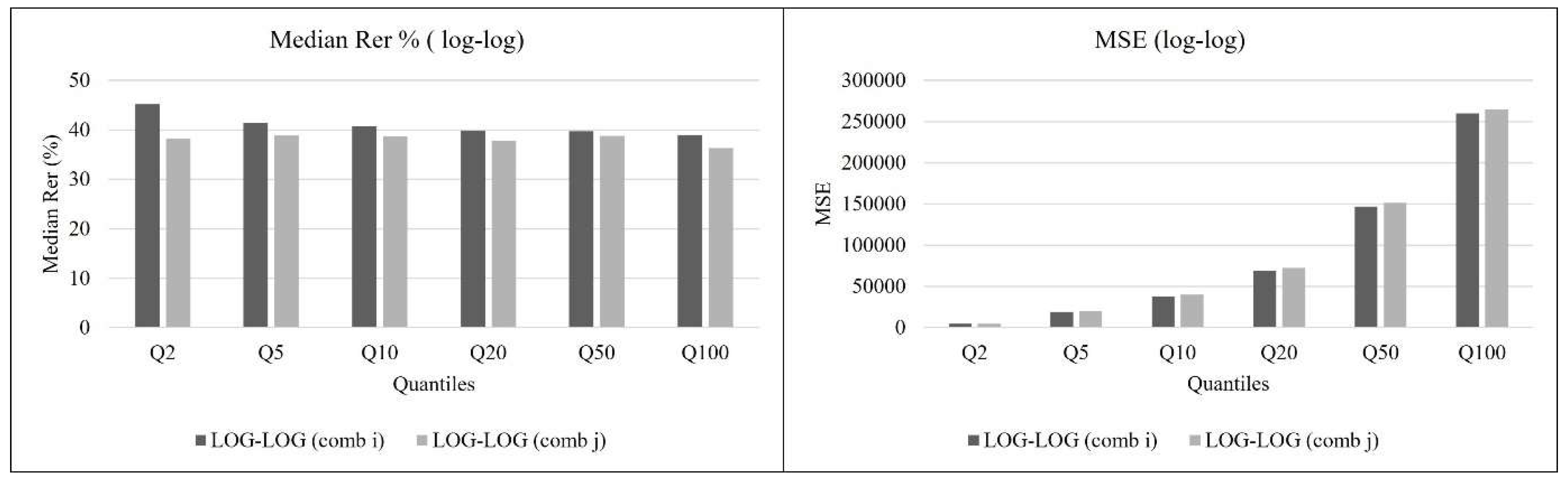
Figure 3.
Boxplots of the ratio for the selected combinations for AEPs of 1 in 2, 5 and 10.
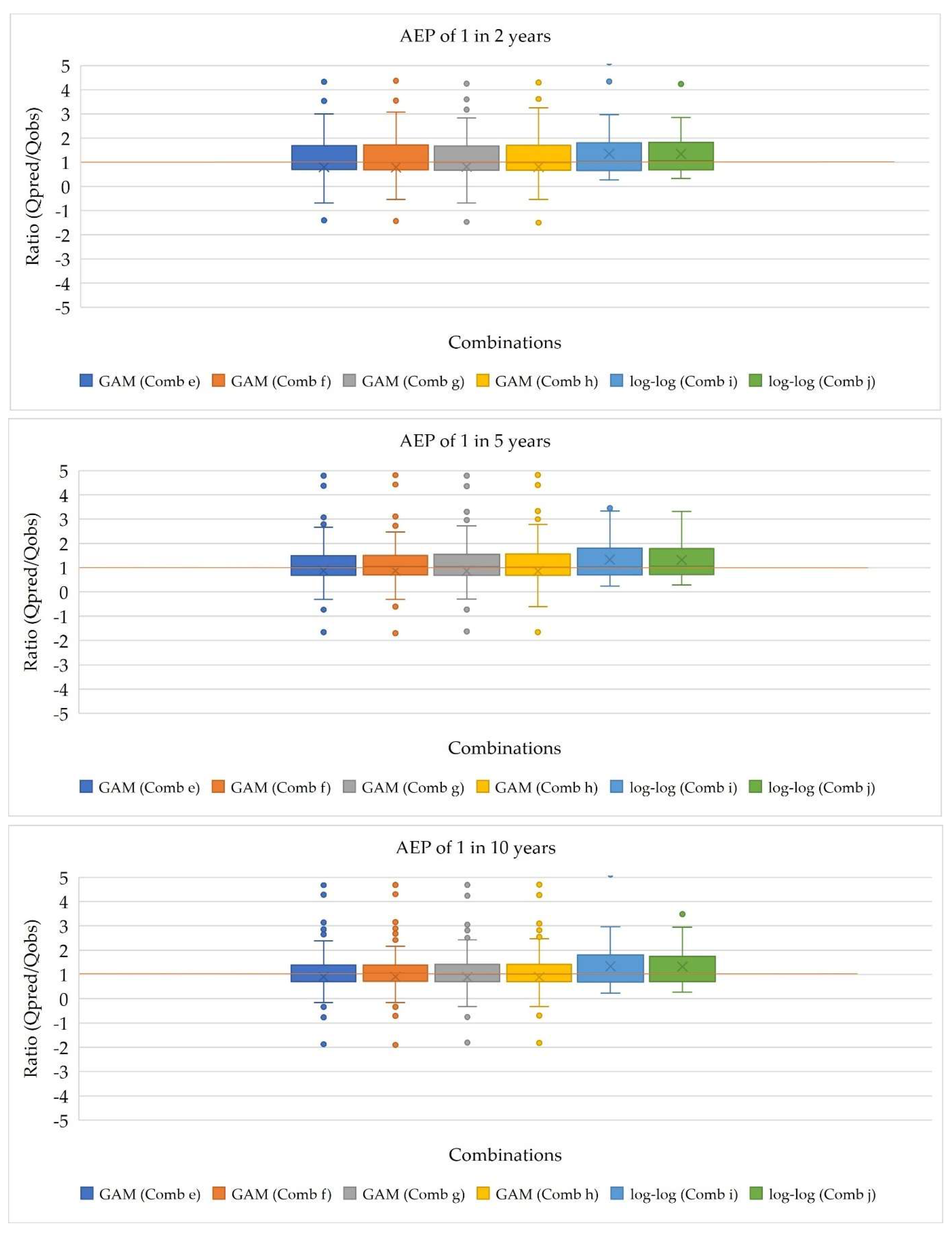
Figure 4.
Boxplots of the ratio for the selected combinations for AEPs of 1 in 20, 50 and 100.
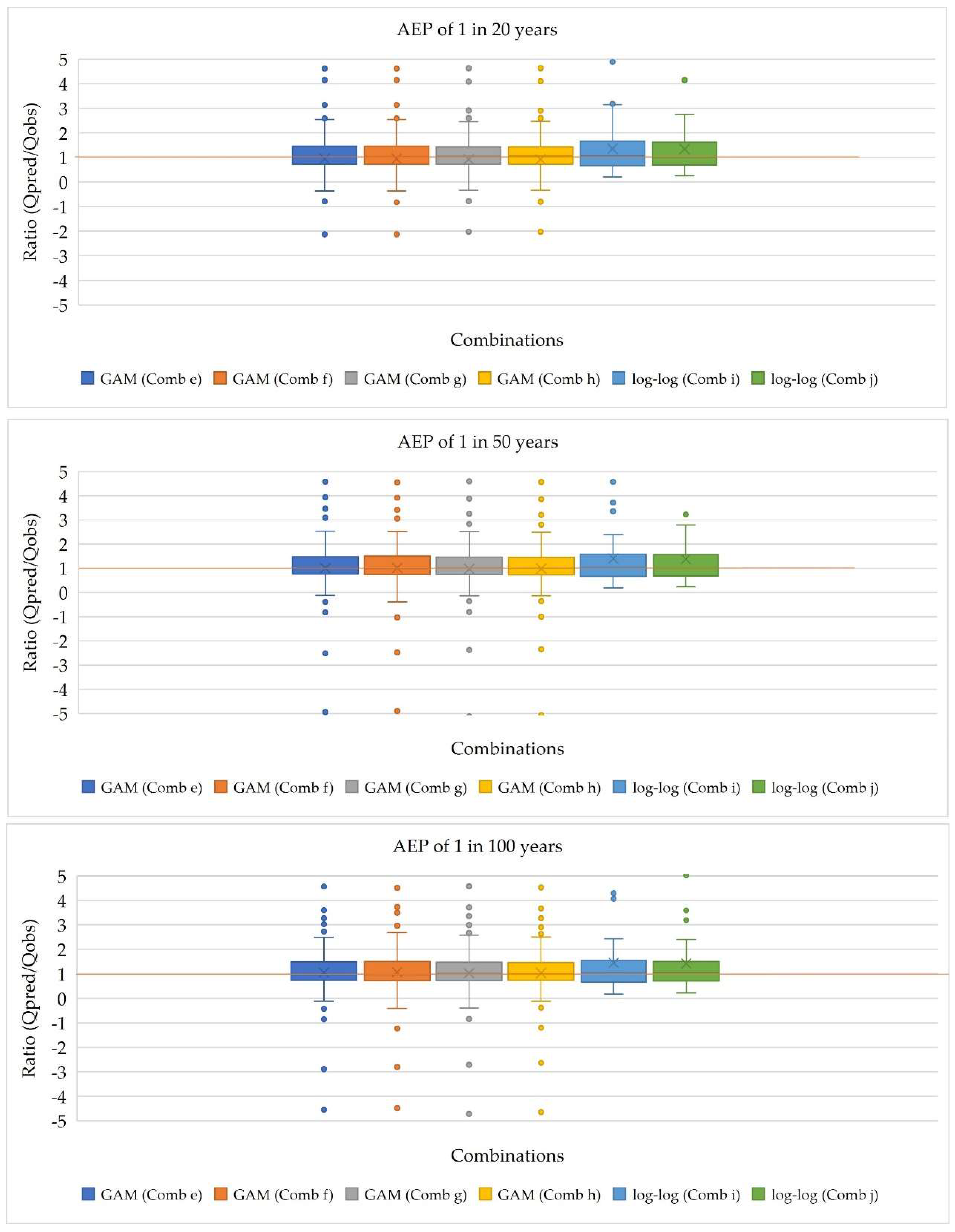
Figure 5.
Boxplots of relative error % for selected combinations for AEPs of 1 in 2, 5 and 10.
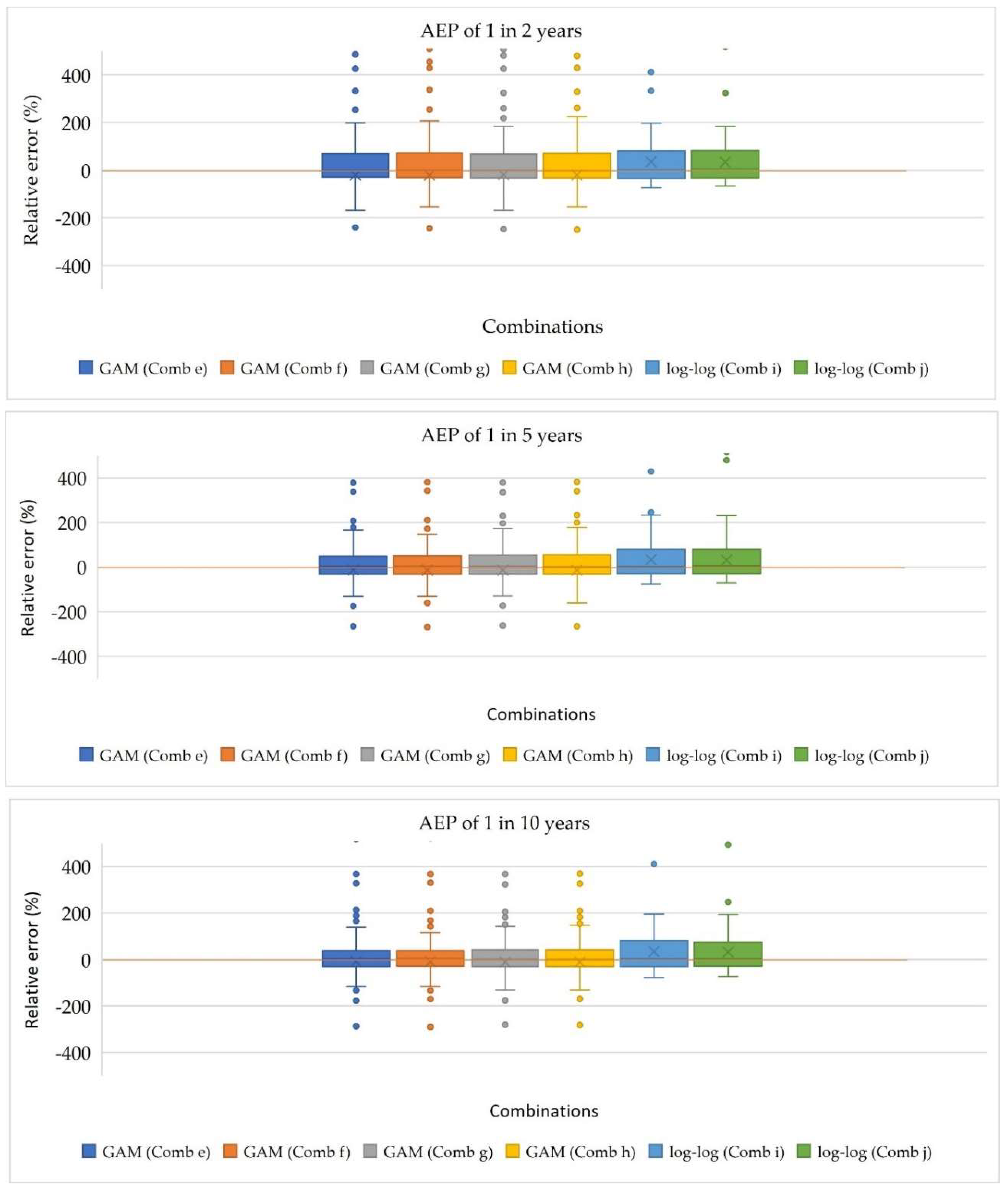
Figure 6.
Boxplots of relative error % for selected combinations for AEPs of 1 in 20, 50 and 100.
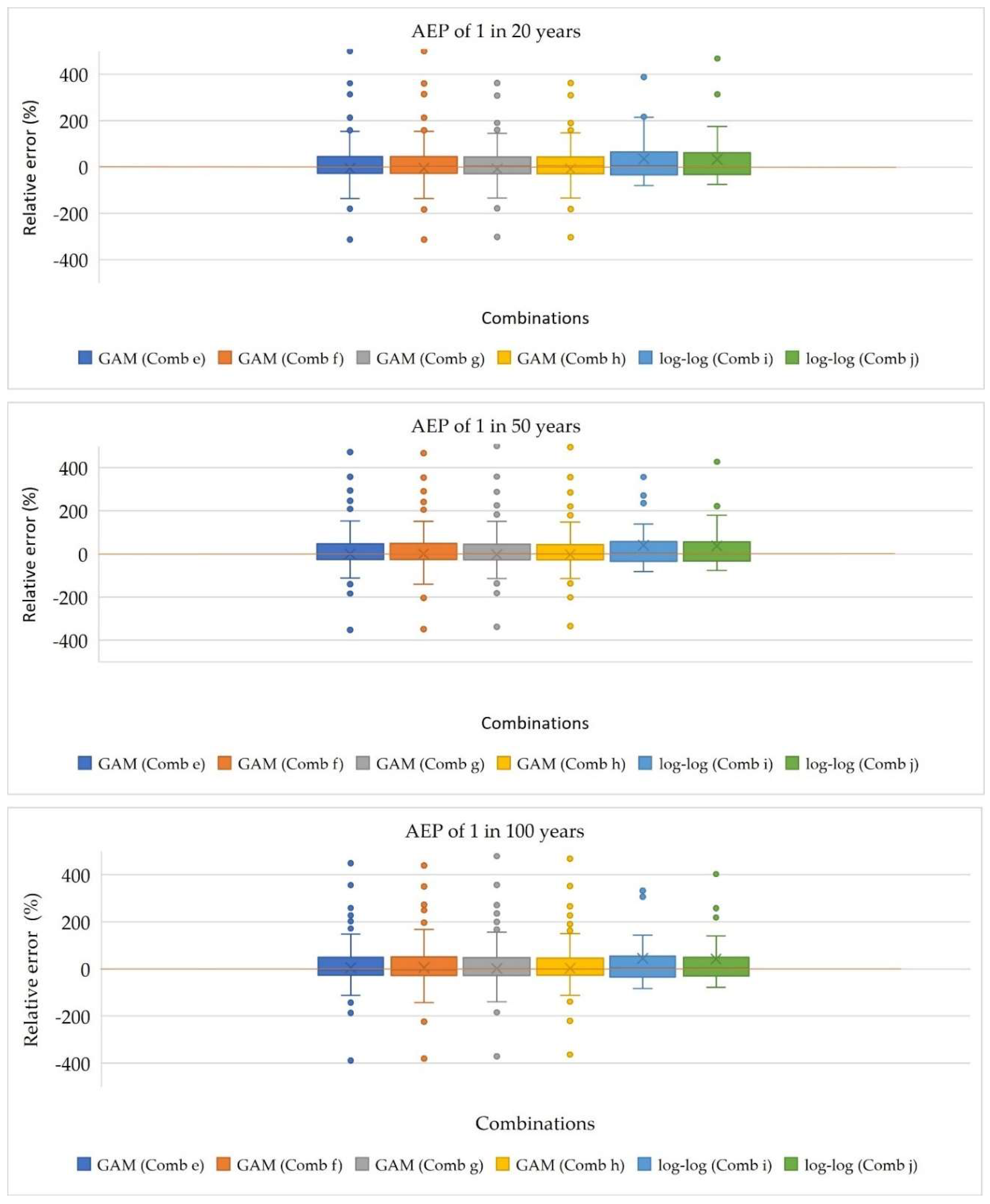
Figure 7.
Median ratio and median REr% values for the selected combinations for AEPs of 1 in 2, 1 in 5, 1 in 10, 1 in 20, 1 in 50 and 1 in 100.
Figure 7.
Median ratio and median REr% values for the selected combinations for AEPs of 1 in 2, 1 in 5, 1 in 10, 1 in 20, 1 in 50 and 1 in 100.
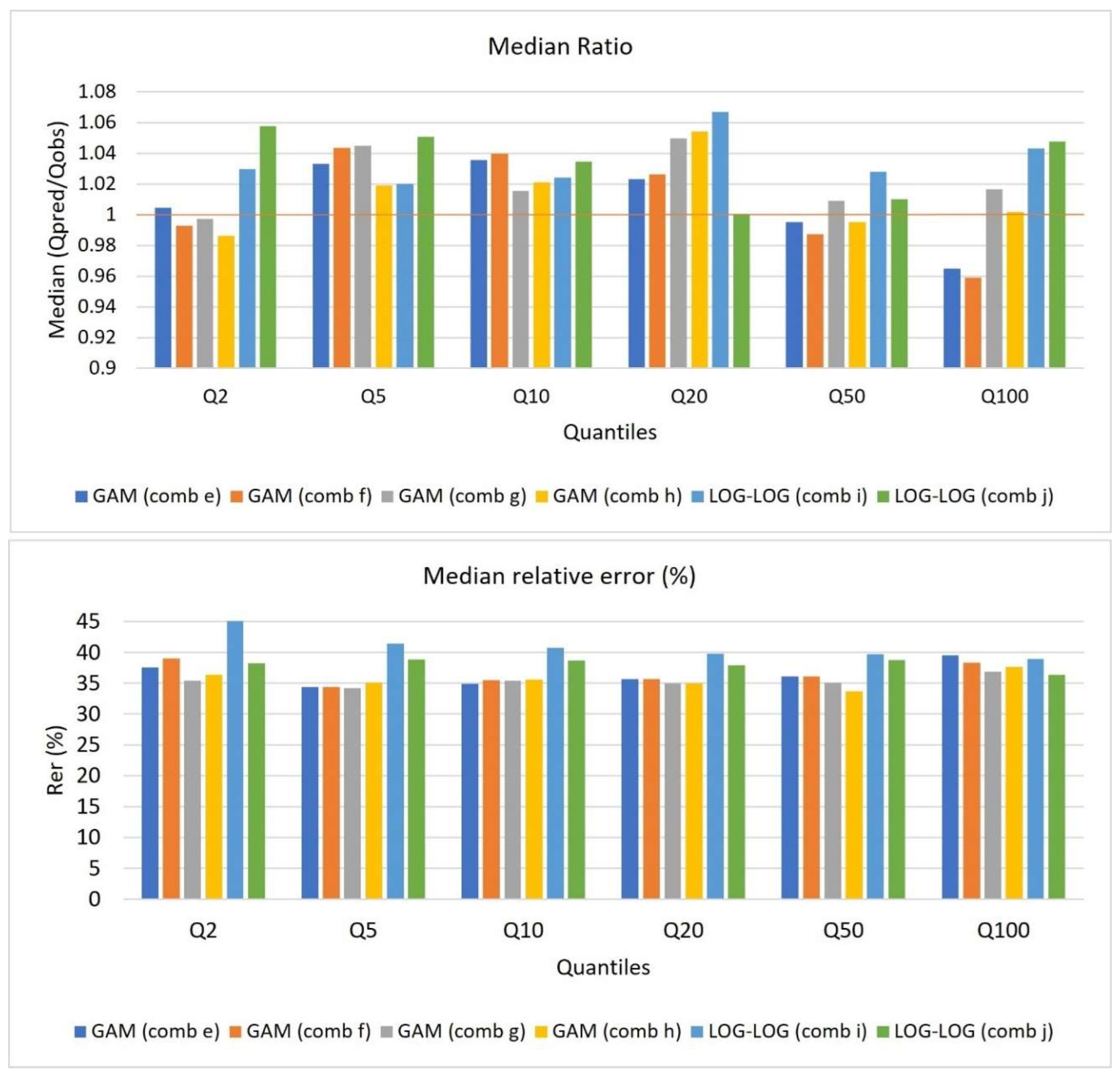

Table 1.
Summary of catchment characteristics data.
| Catchment Characteristics | Min | Max | Mean | Standard deviation |
|---|---|---|---|---|
| Catchment area (km2) | 8 | 1010 | 351.977 | 281.428 |
| I6,2(mm) | 31.400 | 88.500 | 45.360 | 11.213 |
| MAR | 626.170 | 1953.230 | 1000.282 | 304.482 |
| SF | 0.258 | 1.629 | 0.761 | 0.209 |
| MAE | 980.400 | 1543.300 | 1223.686 | 126.303 |
| SDEN | 0.519 | 5.474 | 2.849 | 1.099 |
| S1085 | 1.538 | 49.855 | 12.916 | 10.804 |
| FOREST | 0.010 | 0.990 | 0.506 | 0.315 |
Table 2.
Summary of the GEV parameters for 88 catchments using FLIKE software.
| GEV Parameters | Min | Max | Mean | Standard deviation |
|---|---|---|---|---|
| Location | 0.909 | 460.473 | 74.954 | 78.286 |
| Scale | 1.490 | 409.042 | 84.824 | 85.452 |
| LCV (L2/L1) | 0.316 | 0.743 | 0.545 | 0.096 |
| LSK | 0.037 | 0.695 | 0.390 | 0.128 |
Table 3.
Summary of significant predictor variables identified for estimating mean parameter in GAMs after LOO.
Table 3.
Summary of significant predictor variables identified for estimating mean parameter in GAMs after LOO.
| Models | Response variable | Predictor variables (PVs) | Significant PVs after LOO |
|---|---|---|---|
| Model 1 | Mean | area, I62, SF, MAE | area, I62, MAE |
| Model 2 | Mean | area, I62, MAE, SDEN | area, I62, MAE |
| Model 3 | Mean | area, I62 | area, I62 |
| Model 4 | Mean | area, I62, SF | area, I62 |
| Model 5 | Mean | area, I62, MAR, MAE | area, I62, MAE |
| Model 6 | Mean | area, I62, MAE | area, I62, MAE |
| Model 7 | Mean | area, I62, SF, S1085 | area, I62 |
| Model 8 | Mean | area, I62, SF, SDEN | area, I62 |
Table 4.
Model statistics for eight GAM models estimating mean parameter.
| Mean | R2 | GCV score | AIC | df residual |
|---|---|---|---|---|
| Model 1 | 0.68 | 667894.09 | 1038.96 | 77.59 |
| Model 2 | 0.68 | 639872.12 | 1038.39 | 77.41 |
| Model 3 | 0.60 | 2208814.13 | 1048.34 | 81.34 |
| Model 4 | 0.61 | 1613094.33 | 1048.20 | 80.48 |
| Model 5 | 0.68 | 630028.06 | 1038.99 | 73.81 |
| Model 6 | 0.70 | 483878.03 | 1035.70 | 75.69 |
| Model 7 | 0.62 | 1316201.35 | 1048.30 | 79.87 |
| Model 8 | 0.62 | 1140118.24 | 1049.70 | 79.37 |
Table 5.
Summary of significant predictor variables identified for estimating LCV parameter in GAMs after LOO.
Table 5.
Summary of significant predictor variables identified for estimating LCV parameter in GAMs after LOO.
| Models | Response variable | Predictor variables (PVs) | Significant PVs after LOO |
|---|---|---|---|
| Model 1 | LCV | area, MAR, SF, MAE | MAR, SF, MAE |
| Model 2 | LCV | MAR, SF, MAE, FOREST | MAR, SF, MAE |
| Model 3 | LCV | MAR, SF, MAE | MAR, SF, MAE |
| Model 4 | LCV | I62, MAR, SF, MAE | MAR, SF, MAE |
| Model 5 | LCV | SF, MAE, FOREST | MAE, FOREST |
| Model 6 | LCV | MAR, SF | MAR |
| Model 7 | LCV | I62, SF | I62 |
| Model 8 | LCV | I62 | I62 |
Table 6.
Model statistics for Eight GAM models estimating LCV parameter.
| LCV | R2 | GCV score | AIC | df residual |
|---|---|---|---|---|
| Model1 | 0.57 | 0.11 | -188.13 | 68.07 |
| Model2 | 0.53 | 0.15 | -183.76 | 69.42 |
| Model3 | 0.53 | 0.16 | -184.08 | 70.41 |
| Model4 | 0.52 | 0.17 | -182.67 | 69.98 |
| Model5 | 0.37 | 0.43 | -170.29 | 75.87 |
| Model6 | 0.26 | 3.40 | -170.71 | 83.00 |
| Model7 | 0.22 | 1.79 | -162.03 | 81.32 |
| Model8 | 0.17 | 4.36 | -160.76 | 83.15 |
Table 7.
Summary of significant predictor variables identified for estimating LSK parameter in GAMs after LOO.
Table 7.
Summary of significant predictor variables identified for estimating LSK parameter in GAMs after LOO.
| Models | Response variable | Predictor variables (PVs) | Significant PVs after LOO |
|---|---|---|---|
| Model 1 | LSK | area, MAR, SF, MAE | area, MAR, SF |
| Model 2 | LSK | MAR, SF, MAE, FOREST | SF |
| Model 3 | LSK | MAR, SF, MAE | SF |
| Model 4 | LSK | I62, MAR, SF, MAE | SF |
| Model 5 | LSK | SF, MAE, FOREST | SF, MAE, FOREST |
| Model 6 | LSK | MAR, SF | MAR |
| Model 7 | LSK | I62, SF | I62, SF |
| Model 8 | LSK | I62 | I62 |
Table 8.
Model statistics for Eight GAM models estimating LSK parameter.
| LSK | R2 | GCV score | AIC | df residual |
|---|---|---|---|---|
| Model1 | 0.51 | 0.22 | -142.16 | 69.62 |
| Model2 | 0.41 | 0.48 | -134.47 | 73.36 |
| Model3 | 0.39 | 0.55 | -133.02 | 73.57 |
| Model4 | 0.40 | 0.51 | -133.86 | 72.79 |
| Model5 | 0.36 | 0.75 | -133.77 | 76.40 |
| Model6 | 0.27 | 2.61 | -131.31 | 79.65 |
| Model7 | 0.33 | 1.41 | -134.06 | 79.46 |
| Model8 | 0.17 | 23.17 | -127.02 | 85.00 |
Table 9.
Median ratio and Median REr% for the selected GAM Combinations.
| Median ratio | ||||||
| GAM Combinations | Q2 | Q5 | Q10 | Q20 | Q50 | Q100 |
| (a): Mean (model 3) – LCV (model 8) – LSK (model 7) | 1.071 | 1.064 | 1.080 | 1.083 | 1.053 | 1.059 |
| (b): Mean (model 3) – LCV (model 8) – LSK (model 8) | 1.076 | 1.060 | 1.082 | 1.084 | 1.090 | 1.078 |
| (c): Mean (model 3) – LCV (model 3) – LSK (model 7) | 1.048 | 1.081 | 1.084 | 1.121 | 1.056 | 1.068 |
| (d): Mean (model 3) – LCV (model 3) – LSK (model 8) | 1.061 | 1.081 | 1.081 | 1.121 | 1.102 | 1.070 |
| (e): Mean (model 6) – LCV (model 8) – LSK (model 7) | 1.004 | 1.033 | 1.036 | 1.023 | 0.995 | 0.965 |
| (f): Mean (model 6) – LCV (model 8) – LSK (model 8) | 0.993 | 1.044 | 1.040 | 1.026 | 0.987 | 0.959 |
| (g): Mean (model 6) – LCV (model 3) – LSK (model 7) | 0.997 | 1.045 | 1.016 | 1.050 | 1.009 | 1.017 |
| (h): Mean (model 6) – LCV (model 3) – LSK (model 8) | 0.986 | 1.019 | 1.021 | 1.054 | 0.995 | 1.002 |
| Median REr% | ||||||
| GAM Combinations | Q2 | Q5 | Q10 | Q20 | Q50 | Q100 |
| (a): Mean (model 3) – LCV (model 8) – LSK (model 7) | 47.391 | 46.823 | 40.931 | 43.295 | 48.806 | 50.560 |
| (b): Mean (model 3) – LCV (model 8) – LSK (model 8) | 46.435 | 49.040 | 41.211 | 43.225 | 48.389 | 49.850 |
| (c): Mean (model 3) – LCV (model 3) – LSK (model 7) | 48.974 | 48.413 | 46.928 | 43.198 | 48.474 | 48.282 |
| (d): Mean (model 3) – LCV (model 3) – LSK (model 8) | 48.097 | 49.289 | 47.381 | 43.097 | 48.267 | 46.899 |
| (e): Mean (model 6) – LCV (model 8) – LSK (model 7) | 37.574 | 34.343 | 34.886 | 35.680 | 36.112 | 39.512 |
| (f): Mean (model 6) – LCV (model 8) – LSK (model 8) | 39.037 | 34.400 | 35.496 | 35.624 | 36.078 | 38.334 |
| (g): Mean (model 6) – LCV (model 3) – LSK (model 7) | 35.438 | 34.230 | 35.380 | 34.969 | 35.060 | 36.863 |
| (h): Mean (model 6) – LCV (model 3) – LSK (model 8) | 36.397 | 35.100 | 35.589 | 34.956 | 33.684 | 37.620 |
Table 10.
Summary of significant predictor variables identified for estimating Mean parameter in log-log linear model after LOO.
Table 10.
Summary of significant predictor variables identified for estimating Mean parameter in log-log linear model after LOO.
| Models | Response | Predictor variables (PVs) | Significant PVs after LOO |
|---|---|---|---|
| Model 1 | log(Mean) | log(area), log(I62), log(SF), log(MAE) | log(area), log(I62), log(SF) |
| Model 2 | log(Mean) | log(area), log(I62), log(MAE), log(SDEN) | log(area), log(I62), log(SDEN) |
| Model 3 | log(Mean) | log(area), log(I62) | log(area), log(I62) |
| Model 4 | log(Mean) | log(area), log(I62), log(SF) | log(area), log(I62), log(SF) |
| Model 5 | log(Mean) | log(area), log(I62), log(MAR), log(MAE) | log(area) |
| Model 6 | log(Mean) | log(area), log(I62), log(MAE) | log(area), log(I62) |
| Model 7 | log(Mean) | log(area), log(I62), log(SF), log(S1085) | log(area), log(I62), log(SF) |
| Model 8 | log(Mean) | log(area), log(I62), log(SF), log(SDEN) | log(area), log(I62), log(SF), log(SDEN) |
| Model 9 | log(Mean) | log(area), log(I62), log(MAR), log(SF), log(MAE), log(SDEN), log(S1085), log(FOREST) | log(area), log(I62), log(SF), log(SDEN) |
Table 11.
Model statistics for nine log-log linear models estimating Mean parameter.
| Model | R2 | AIC | BIC |
|---|---|---|---|
| 1 | 0.77 | 150.86 | 165.72 |
| 2 | 0.77 | 149.59 | 164.45 |
| 3 | 0.75 | 152.60 | 162.51 |
| 4 | 0.76 | 149.61 | 162.00 |
| 5 | 0.75 | 155.22 | 170.09 |
| 6 | 0.75 | 153.44 | 165.83 |
| 7 | 0.77 | 149.31 | 164.17 |
| 8 | 0.78 | 146.56 | 161.43 |
| 9 | 0.79 | 151.29 | 176.06 |
Table 12.
Summary of significant predictor variables identified for estimating LCV parameter in log-log linear after LOO.
Table 12.
Summary of significant predictor variables identified for estimating LCV parameter in log-log linear after LOO.
| Models | Response | Predictor variables (PVs) | Significant PVs after LOO |
|---|---|---|---|
| Model 1 | LCV | log(area), log(MAR), log(SF), log(MAE) | log(MAR) |
| Model 2 | LCV | log(MAR), log(SF), log(MAE), log(FOREST) | log(MAR) |
| Model 3 | LCV | log(MAR), log(SF), log(MAE) | log(MAR) |
| Model 4 | LCV | log(I62), log(MAR), log(SF), log(MAE) | log(MAR) |
| Model 5 | LCV | log(SF), log(MAE), log(FOREST) | log(MAE) - log(FOREST) |
| Model 6 | LCV | log(MAR), log(SF) | log(MAR) |
| Model 7 | LCV | log(I62), log(SF) | log(I62) |
| Model 8 | LCV | log(I62) | log(I62) |
| Model 9 | LCV | log(area), log(I62), log(MAR), log(SF), log(MAE), log(SDEN), log(S1085), log(FOREST) | log(MAR) |
Table 13.
Model statistics for nine log-log linear models estimating LCV parameter.
| Model | R2 | AIC | BIC |
|---|---|---|---|
| 1 | 0.22 | -166.26 | -151.39 |
| 2 | 0.24 | -167.91 | -153.05 |
| 3 | 0.22 | -168.25 | -155.87 |
| 4 | 0.23 | -167.55 | -152.69 |
| 5 | 0.13 | -158.20 | -145.81 |
| 6 | 0.22 | -169.90 | -159.99 |
| 7 | 0.09 | -156.14 | -146.23 |
| 8 | 0.09 | -158.01 | -150.58 |
| 9 | 0.26 | -162.13 | -137.36 |
Table 14.
Summary of significant predictor variables identified for estimating LSK parameter in log-log linear after LOO.
Table 14.
Summary of significant predictor variables identified for estimating LSK parameter in log-log linear after LOO.
| Models | Response | Predictor variables (PVs) | Significant PVs after LOO |
|---|---|---|---|
| Model 1 | LSK | log(I62), log(SF), log(MAE) | log(I62) |
| Model 2 | LSK | log(I62), log(SF), log(SDEN) | log(I62) |
| Model 3 | LSK | log(I62), log(SF), log(FOREST) | log(I62) |
| Model 4 | LSK | log(I62), log(SF) | log(I62) |
| Model 5 | LSK | log(I62), log(SDEN) | log(I62) |
| Model 6 | LSK | log(I62), log(MAE) | log(I62) |
| Model 7 | LSK | log(I62), log(S1085) | log(I62) |
| Model 8 | LSK | log(I62) | log(I62) |
| Model 9 | LSK | log(area), log(I62), log(MAR), log(SF), log(MAE), log(SDEN), log(S1085), log(FOREST) | none |
Table 15.
Model statistics for nine log-log linear models estimating LSK parameter.
| Model | R2 | AIC | BIC |
|---|---|---|---|
| 1 | 0.16 | -124.18 | -111.80 |
| 2 | 0.17 | -124.94 | -112.55 |
| 3 | 0.18 | -126.00 | -113.61 |
| 4 | 0.16 | -126.14 | -116.23 |
| 5 | 0.16 | -126.32 | -116.41 |
| 6 | 0.16 | -125.55 | -115.64 |
| 7 | 0.16 | -125.59 | -115.68 |
| 8 | 0.16 | -127.54 | -120.11 |
| 9 | 0.20 | -118.14 | -93.37 |
Table 16.
Summary of percentage median REr% for GAM and log-log linear models.
| Median REr% | ||||||
|---|---|---|---|---|---|---|
| Q2 | Q5 | Q10 | Q20 | Q50 | Q100 | |
| min (GAM) | 35.44 | 34.23 | 34.89 | 34.96 | 33.68 | 36.86 |
| min (log-log) | 38.26 | 38.84 | 38.65 | 37.88 | 38.78 | 36.32 |
| max (GAM) | 39.04 | 35.10 | 35.59 | 35.68 | 36.11 | 39.51 |
| max (log-log) | 45.19 | 41.41 | 40.74 | 39.79 | 39.74 | 38.92 |
Table 17.
Quantile Evaluation: rBIAS (%) and rRMSE (%) for the selected model combinations.
| Quantiles | GAM (e) | GAM (f) | GAM (g) | GAM (h) | log-log (i) | log-log (j) | |
|---|---|---|---|---|---|---|---|
| rBIAS (%) | Q2 | -20.74 | -19.03 | -19.41 | -19.41 | 34.95 | 34.02 |
| Q5 | -13.31 | -13.91 | -14.16 | -14.16 | 32.75 | 31.63 | |
| Q10 | -9.47 | -10.93 | -11.07 | -11.07 | 33.48 | 32.15 | |
| Q20 | -5.49 | -7.68 | -7.64 | -7.64 | 35.37 | 33.75 | |
| Q50 | 0.75 | -2.50 | -2.04 | -2.04 | 39.80 | 37.70 | |
| Q100 | 6.43 | 2.15 | 3.15 | 3.15 | 44.95 | 42.37 | |
| rRMSE (%) | Q2 | 62.45 | 62.73 | 61.64 | 61.92 | 62.35 | 65.32 |
| Q5 | 58.42 | 58.82 | 58.81 | 59.22 | 59.39 | 61.69 | |
| Q10 | 56.91 | 57.19 | 57.29 | 57.58 | 57.81 | 59.68 | |
| Q20 | 56.34 | 56.37 | 56.49 | 56.52 | 56.84 | 58.30 | |
| Q50 | 57.03 | 56.59 | 56.69 | 56.22 | 56.71 | 57.65 | |
| Q100 | 58.63 | 57.78 | 57.85 | 56.95 | 57.62 | 58.21 |
Disclaimer/Publisher’s Note: The statements, opinions and data contained in all publications are solely those of the individual author(s) and contributor(s) and not of MDPI and/or the editor(s). MDPI and/or the editor(s) disclaim responsibility for any injury to people or property resulting from any ideas, methods, instructions or products referred to in the content. |
© 2024 by the authors. Licensee MDPI, Basel, Switzerland. This article is an open access article distributed under the terms and conditions of the Creative Commons Attribution (CC BY) license (http://creativecommons.org/licenses/by/4.0/).
Copyright: This open access article is published under a Creative Commons CC BY 4.0 license, which permit the free download, distribution, and reuse, provided that the author and preprint are cited in any reuse.


