Submitted:
19 December 2024
Posted:
20 December 2024
Read the latest preprint version here
Abstract
Human Activity Recognition (HAR) and gender recognition have become pivotal in advancing intelligent systems, as they enable tailored user experiences and enhance automation in healthcare, security, and personalized technology. By accurately identifying human activities and gender, systems can proactively adapt to user needs, improving human-computer interaction, reducing response times in emergency detection, and enhancing the quality of life in smart home and assistive living applications. In this study, a Kolmogorov-Arnold Network model was created to predict daily living activities and the gender of the person performing an activity. The proposed Kolmogorov-Arnold Network (KAN) classifier outperformed the previous studies with 94.5% and 95.6% in terms of overall accuracy for multi-class HAR and gender recognition tasks, respectively. Additionally, the Chi-square test results demonstrated that there is a statistically significant difference between the performances. It can be concluded that KAN method is a robust classifier especially for detecting activities that have a minor number of samples on the utilized dataset.
Keywords:
activity recognition
; gender recognition
; machine learning
; artificial intelligence
; neural networks
; Kolmogorov-Arnold networks
1. Introduction
Human Activity Recognition (HAR) has become a prominent area of research in recent years due to its wide range of applications, including healthcare monitoring, assisted living, sports analytics, and human-computer interaction. HAR systems aim to automatically classify human activities, such as walking, running, or sitting, using sensor data from wearable devices like smartphones and smartwatches [1,2]. These systems provide valuable insights for various domains, from detecting falls in elderly individuals to monitoring physical activity levels for fitness applications [3]. Examples of application areas can be expanded. A HAR system can be developed for detecting unauthorized access in home security systems, ensuring workplace safety in industrial environments, or for use in military applications [4,5]. It can be used to create natural and intuitive user interfaces. In this way, devices can be controlled through gestures or body movements [6]. In augmented reality applications, it can be beneficial for understanding the user's interaction with the physical environment and accordingly placing virtual objects [7].
There are also challenges in developing a HAR system. People may exhibit different movements in various environments and on different devices. This increases the diversity of datasets and makes the classification task more challenging [8]. There may be noise and uncertainties in sensor data, which can hinder the accurate recognition of movements. Especially in real-time applications, high computational power may be required to process large amounts of data quickly [9].
A key motivation behind HAR is the proliferation of wearable sensor devices, which have enabled the continuous and real-time collection of data. Wearable sensors, such as accelerometers, gyroscopes, and magnetometers, have become integral to modern HAR systems, offering an affordable and scalable way to capture human motion [10]. With the availability of these devices, researchers have explored various machine learning and deep learning techniques to improve the accuracy and efficiency of activity recognition models.
Several studies have demonstrated the potential of canonical machine learning algorithms in HAR. For instance, Banos et al. [10] investigated the impact of window size on activity recognition performance by utilizing decision trees (DT), k-nearest neighbours (kNN), Naïve Bayes (NB), and nearest centroid classifier (NCC). The study focused on a wide range of fitness activities, which were categorized under warm-up, cool-down and fitness exercises. Three sets of features were extracted to feed the classifiers and kNN was the highest-performing classifier with an F1-score of 0.95 to 1 for certain activities and feature sets. This study addressed the gap in the literature regarding the lack of formal studies on appropriate window size selection for accurate recognition. It offered design guidelines for determining optimal window size to balance recognition speed and accuracy, depending on the complexity of the activity and the richness of the feature set.
Anguita et al. [11] presented a public HAR dataset and used support vector machines (SVM) to achieve high recognition rates for six basic activities like walking, standing, sitting, laying down, walking downstairs, and walking upstairs. Time and frequency domain signals were obtained from the smartphone sensors including accelerometer and gyroscope data. The SVM classifier achieved an accuracy with an overall recognition rate of 96%. The article contributed a publicly available HAR dataset using smartphones. Additionally, the study showed that smartphones, which are more unobtrusive and less invasive than special-purpose sensors, can be effectively used for human activity recognition tasks with high accuracy.
Gupta and Dallas [12] focused on classifying six daily activities: walking, running, jumping, sit-to-stand/stand-to-sit transitions, stand-to-kneel-to-stand transitions, and being stationary (sitting or standing). The study employed two classifiers, which were kNN and NB. Features were computed from accelerometer data, focusing on time-domain analysis, as the data was segmented into 6-second windows. After extracting features, some features were selected by utilizing Relief-F and sequential forward floating search algorithms. Both classifiers achieved an overall accuracy of about 98%, with more than 95% accuracy for individual activities. This study introduced new features like mean trend, windowed mean difference, and detrended fluctuation analysis, which improved classification performance for HAR. It proposed a system that reduces the dependency on sensor orientation and position around the waist, making it more practical for real-life applications with minimal user training. Additionally, it addressed a gap in prior studies that often excluded transitions by demonstrating high classification accuracy for daily activities and transitional events.
Reyes-Ortiz et al. [13] proposed a system targeting various physical activities and transitions including walking, sitting, standing, lying down, walking upstairs, and walking downstairs. Additionally, postural transitions like sit-to-stand and stand-to-sit were included. SVM with probabilistic outputs were used to classify the activities. Both time-domain and frequency-domain features were extracted from the smartphone's triaxial accelerometer and gyroscope signals. The paper mentioned that the proposed system outperformed state-of-the-art baseline methods. The architecture improved classification by combining SVM outputs with heuristic filters, which was an innovative approach in the field.
Catal et al. [14] utilized an ensemble of classifiers including DT, multi-layer perceptron (MLP), and logistic regression. The proposed ensemble method combined the classifiers using the average of probabilities combination rule. The activities they aimed to predict were walking, jogging, upstairs, downstairs, sitting, and standing. Time-domain features were extracted from accelerometer data to feed the classifiers. The highest accuracy was achieved by their proposed ensemble model, outperforming standalone classifiers. This study suggested that the ensemble approach could be particularly effective for complex activities and provided a strong baseline for future research in activity recognition using mobile devices.
Demrozi et al. [15] focused on detecting freezing of gait (FoG) episodes in people with Parkinson's Disease instead of predicting daily activities. The study used kNN machine learning model to detect FoG episodes. Data were obtained from three tri-axial accelerometer sensors. The features were extracted by applying windowing and dimensionality reduction techniques. The research contributed to the field by integrating wearable technology and machine learning to address a critical health issue in Parkinson's disease management.
Climent-Pérez et al. [16] focused on recognizing daily human activities while hiding gender and age. A many-objective evolutionary algorithm was utilized for feature weighting, and RF was utilized for classification. Both time and frequency domain features were extracted from accelerometer data to feed the classifier. The article made a significant contribution by utilizing an optimization algorithm to tackle the dual challenges of high-accuracy activity recognition and privacy preservation.
Asuroglu [17] proposed a locally weighted random forest classifier (LWRF), which outperformed Climent-Perez et al.’s [16] study in terms of overall accuracy that utilized random forest (RF) classifier on the same dataset. Additionally, the study benchmarked other machine learning algorithms including DT, MLP, kNN, NB, Logistic Model Tree (LMT), and SVM. The proposed model achieved the highest accuracy, with 91% for human activity recognition and 91.3% for gender recognition among the mentioned classifiers. This study introduced the first use of a local weighted approach in the domain of accelerometer signal-based human activity recognition. It improved upon the Random Forest classifier by adding local weighting to address dataset variability and achieved higher accuracy in predicting complex human activities compared to previous methods. Additionally, the study provided a robust framework for recognizing activities with a limited number of samples.
Garcia-Gonzalez et al.’s [18] study focused on four types of human activities: inactive, active, walking, and driving. The authors employed various machine learning models, including SVM, DT, MLP, NB, kNN, RF, and Extreme Gradient Boosting (XGB). Both time-domain features and specific proposed additions such as total distance travelled and energy, based on data from accelerometer, gyroscope, magnetometer, and GPS sensors, were extracted to feed the classifiers. The features were extracted using a sliding window method with windows ranging from 20 to 90 seconds. RF outperformed the other algorithms, achieving the highest accuracy of 92.97%. This paper contributed to the literature by comparing different machine learning algorithms using real-life smartphone sensor data rather than laboratory-collected data. It also introduced the use of XGB in human activity recognition and evaluated the impact of excluding gyroscope data from the sensors.
In recent years, the focus of HAR research has shifted towards deep learning, multimodal and multi-sensor fusion approaches. Ordóñez and Roggen [19] studied on recognizing human activities from multimodal wearable sensors, including static/periodic activities such as modes of locomotion and postures, as well as sporadic activities like gestures. In the study, a combination of Convolutional Neural Networks (CNN) and Long Short-Term Memory (LSTM) recurrent layers, referred to as the DeepConvLSTM model, was utilized. The features were learned automatically through the convolutional and recurrent layers without manual feature engineering. The raw sensor data were processed from wearable devices, such as accelerometers, gyroscopes, and magnetic sensors. The model learned both spatial and temporal dependencies in the sensor signals. The DeepConvLSTM model achieved an improvement in accuracy, outperforming previous state-of-the-art methods by up to 9%. Specifically, the F1-score of 0.930 for locomotion recognition and 0.915 for gesture recognition showed its superiority. The contribution of this paper lied in the combination of CNNs and LSTM layers for human activity recognition. This allowed for both automatic feature extraction and capturing temporal dependencies in the data. The paper also showed that this architecture is well-suited for fusing multimodal sensor data, making it highly applicable in real-life HAR scenarios. The paper outperformed existing methods on benchmark datasets (OPPORTUNITY and Skoda) and provided a robust analysis of hyperparameter tuning to further improve performance.
Similarly, Yang et al. [20] utilized CNNs for HAR tasks and showed that these models can effectively capture spatial and temporal dependencies in sensor data. Their paper focused on recognizing human activities, such as walking, running, sitting, and other common daily movements from multichannel time series data collected through wearable devices. The paper proposed the use of deep CNN (DCNNs) as the classifier for time-series data. The authors leveraged CNNs due to their effectiveness in automatically learning spatial hierarchies from raw sensor data. The paper did not rely on manual feature extraction. Instead, features were automatically learned by the convolutional layers of the deep network, which processed the raw multichannel time series data from wearable sensors such as accelerometers and gyroscopes. The DCNN achieved the highest accuracy in the experiments, significantly outperforming traditional machine learning methods like kNN and DT. The exact accuracy metrics depend on the dataset used, but the DCNN demonstrated superior performance across multiple datasets. This paper made a substantial contribution by applying DCNNs to multichannel time series data, which was a novel approach at the time of publication. The proposed method also addressed the challenge of dealing with high-dimensional data streams generated by wearable sensors, making it a highly applicable solution in real-life HAR scenarios.
The use of deep learning models, particularly CNNs and recurrent neural networks (RNNs), has gained attention due to their ability to learn hierarchical features directly from raw sensor data, reducing the need for handcrafted features.
DeepSense, a unified deep learning framework developed by Yao et al. [21], leveraged CNNs to process time-series sensor data for HAR, achieving competitive results across multiple datasets. The paper focused on a variety of tasks including car tracking, human activity recognition, and user identification based on time-series data from mobile sensors such as accelerometers, gyroscopes, and magnetometers. The framework combined CNNs and recurrent neural networks (RNNs). CNNs were used for extracting spatial features from raw sensor data, while RNNs captured the temporal dependencies across time-series data. This approach eliminated the need for manual feature engineering. DeepSense outperformed other methods and achieved state-of-the-art results across multiple tasks. For car tracking, it had a Mean Absolute Error (MAE) of approximately 1.4 meters. For human activity recognition, it achieved an accuracy of up to 95%. For user identification, the accuracy reached up to 96%. The framework was also optimized for deployment on mobile devices, demonstrating feasibility in terms of computation and energy consumption. This made it a versatile and practical solution for real-world sensing applications.
In another study, Ignatov [22] introduced a real-time HAR system based on CNNs, which was optimized for smartphone accelerometer data, achieving high classification accuracy. The paper focused on recognizing human activities such as walking, jogging, standing, sitting, walking upstairs, and walking downstairs using accelerometer data from smartphones. The proposed system achieved an accuracy of 96.75% and 94.8%, outperforming other models, on the WISDM dataset and UCI HAR dataset, respectively. This study contributed by demonstrating that CNNs, when combined with statistical features from time-series data, can achieve real-time performance with low computational cost. The paper also highlighted that the system can process 1-second time windows in real time, making it highly suitable for continuous monitoring in activity recognition systems.
The integration of deep learning methods has significantly improved the robustness and scalability of HAR systems, particularly in real-world applications where noise and variability in sensor data can pose challenges.
Guan and Plötz [23] aimed to predict human activities such as walking, running, sitting, standing, lying down, and other activities typically captured by wearable sensors. The study employed an ensemble of LSTM learners due to their ability to capture long-range dependencies for time-series data. No manual feature extraction was involved, as the LSTM learns temporal and sequential patterns from raw sensor data recorded by accelerometers, gyroscopes, and magnetometers. The ensemble of LSTM learners achieved the best performance, outperforming single LSTM models and other deep learning methods. The exact accuracy varied depending on the dataset, but it consistently improved performance on benchmarks like the Opportunity, PAMAP2, and Skoda datasets. The ensemble method was particularly effective in improving accuracy in the presence of noisy and imbalanced data. The paper introduced the concept of epoch-wise bagging to generate multiple diverse LSTM models, which improves the generalization of the ensemble model.
Murad and Pyun [24] targeted to predict a wide range of human activities, depending on the dataset used, such as walking, running, ascending/descending stairs, standing, sitting, laying, and other daily activities. The study proposed and implemented several deep recurrent neural network (DRNN) architectures based on LSTM, including unidirectional LSTM-based DRNN, bidirectional LSTM-based DRNN, and cascaded bidirectional and unidirectional LSTM-based DRNN. The models used raw multimodal sensor data collected from accelerometers, gyroscopes, and magnetometers. The data was fed into the networks without any handcrafted features. The bidirectional LSTM-based DRNN yielded the best performance on complex datasets like the Opportunity dataset, while the unidirectional DRNN performed best on the UCI-HAD and USC-HAD datasets. For UCI-HAD, the overall classification accuracy reached 96.7%, and for USC-HAD, it reached 97.8%. The study introduced models capable of handling variable-length input sequences. Additionally, it demonstrated superior performance of DRNNs compared to both traditional machine learning classifiers like SVM and kNN and other deep learning approaches like CNN and deep belief networks.
Hu et al. [25] used LSTM and gated recurrent unit (GRU) to model time-series sensor data and capture temporal dependencies in human activity. No manual feature extraction was performed, as the raw sensor data from accelerometers and gyroscopes is fed directly into the LSTM layers, allowing the network to automatically learn spatial and temporal features. The harmonic loss function applied to LSTM and GRU outperformed other traditional loss functions like cross-entropy loss and focal loss, especially on imbalanced datasets. The contribution of the study to the literature is to introduce a novel harmonic loss function and improve classification accuracy and macro-F1 scores for HAR, particularly on imbalanced datasets, which is a common issue in real-world sensor-based HAR applications.
To the best of our knowledge, this study is the first one that utilizes Kolmogorov-Arnold Network (KAN) on HAR and gender recognition. A minor contribution is that one-versus-all classifications for 24 classes were performed on the PAAL ADL Accelerometery dataset v2.0 [26]. Additionally, statistical methods were applied to detect the statical significance between the previous methods.
The motivation for employing the KAN method can be elucidated within the context of the data. The dataset, utilized in this study, contains significant class imbalances, with certain activities (e.g., sneezing/coughing, brushing hair) having far fewer samples compared to others (e.g., making a phone call, writing). This imbalance poses challenges for traditional classifiers, which often struggle to maintain performance for minority classes. KAN’s adaptive spline-based activation functions may enable it to model non-linear relationships effectively, even for classes with fewer samples. This adaptability may help it outperform traditional machine learning models in recognizing minority class activities. Variations in how participants perform the same activity (e.g., putting on glasses or standing up) introduce noise and increase the complexity of classification tasks. Additionally, the dataset spans a broad demographic, with participants aged 18–77 years, including both genders. This diversity enriches the dataset but also adds to the complexity of classification tasks. KAN’s architecture may help at capturing complex dependencies in multi-dimensional data, such as the combined time-domain and frequency-domain features extracted from accelerometer signals. Unlike traditional neural networks with fixed activation functions, KAN’s learnable activation functions may allow for dynamic adjustments based on the data, making it particularly suited for datasets with high variability and noise. Finally, by leveraging the Kolmogorov-Arnold representation theorem, KAN may provide a robust framework for function approximation, helping to reduce overfitting, which is a risk in datasets with class imbalance and noise.
The rest of the paper is organized as follows; Section 2 gives information about the utilized dataset, preprocessing steps, and general definition of KAN. In section 3, evaluation metrics, experimental setup, and empirical results are demonstrated. In section 4, discussion for the empirical results is presented and the article is concluded.
2. Materials and Methods
2.1. Dataset
The dataset utilized in this study is publicly available at https://zenodo.org/record/5785955 [26]. There are 52 participants in total, comprising 26 men and 26 women. The participants' ages are distributed across different age groups. The age range is between 18 and 77 years. The average age of the participants in the study is 44.08, with a standard deviation of 17.06, years. The data was collected in Spain, particularly in Alicante province, at various locations such as participants' homes or workplaces. The dataset includes 24 different activities of daily living. These are drinking water, eating meal, opening a bottle, opening a box, brushing teeth, brushing hair, taking off jacket, putting on jacket, putting on a shoe, taking off a shoe, putting on glasses, taking off glasses, sitting down, standing up, writing, making a phone call, typing on a keyboard, saluting, sneezing/coughing, blowing nose, washing hands, dusting, ironing, and washing dishes.
A total of 6,072 files were collected, with up to 5 repetitions of each activity per participant by using the Empatica E4 wrist-worn device. The Empatica E4 is equipped with an accelerometer (used for motion tracking), as well as various sensors measuring blood volume pulse, skin temperature and electrodermal activity. The E4 device records accelerometer data at 32 Hz, ensuring a good temporal resolution for capturing subtle movements. The Empatica E4 was primarily designed for continuous, non-invasive monitoring, making it ideal for health and activity research. The accelerometer in the E4 device was used to collect 3D (x, y, and z axis) acceleration signals, which are crucial for recognizing physical activities based on wrist motion. Table 1 shows the class labels, daily living activities, and the number of samples that belong to each activity. The class labels, used in this study, were prepared considering Asuroglu’s study [17] to ensure consistency for prediction tasks. As can be seen from Table 1, the dataset is imbalanced.
To make data available for feature extraction, a two-step process is employed. First, a fourth-order Butterworth low-pass filter with a 15Hz cutoff frequency is applied to retain motion characteristics while filtering out high-frequency noise. Then, a third-order median filter removes outliers. Data are segmented into windows with a 5-second sliding window, overlapping by 20%, yielding 28,642 samples for feature extraction [17].
2.2. General Framework
The aim of this study is to predict human activities and classify gender from accelerometer data utilizing Kolmogorov-Arnold Network (KAN) classifier. The first step involves extracting time-domain and frequency-domain features from 3D accelerometer data. Next, these time and frequency features are combined to obtain a feature vector, which feeds the KAN classifier as input. A standardization process, also known as z-score normalization, is applied to the features so that each feature has a mean of 0 and a standard deviation of 1. To train a KAN model, the 10-fold cross validation technique is utilized. Additionally, a grid search approach is employed to optimize the hyper-parameters of the KAN model, maximizing the overall accuracy evaluation metric. Once the models for both multi-class HAR and gender recognition tasks are obtained, a query sample is provided to the classifiers to predict the activity and the gender in which the individual is engaged and belongs, respectively. The general framework of the proposed method is shown in Figure 1.
2.3. Feature Extraction
Feeding raw accelerometer signal values directly into the proposed classification framework is impractical for several reasons. First, most machine learning classifiers require equal-length input, which accelerometer signals do not provide, as they vary in length [27]. Additionally, even when signals have the same length, they may not align in the same time dimension, complicating the classification process [28]. This variability makes preprocessing necessary before applying machine learning algorithms to accelerometer data.
In two previous studies [16,17], various time and frequency domain features were extracted from raw accelerometer signals to capture essential motion characteristics. This study adopts the same approach as previous works, extracting features from the x, y, and z channels of the accelerometer, along with the signal magnitude vector (SMV). In total, 62 features are extracted from these channels and vectors. The extracted features for time-domain are: mean, median, standard deviation (, maximum, minimum, and range (for x, y, z axes and SMV); correlation between axes (x-y, y-z, and z-x), signal magnitude area (for SMV); coefficient of variation and median absolute deviation (for x, y, z axes and SMV); skewness, kurtosis, autocorrelation, interquartile range, 20th, 50th, 80th, 90th percentiles, number of peaks, peak to peak amplitude, energy, and root mean square (for SMV). The extracted features for frequency-domain are: spectral entropy, energy, and centroid (for SMV); mean and (for x, y, z axes and SMV); 25th, 50th, and 75th percentiles (for SMV). As a result, 62 features were utilized as samples to feed the classifier, where 48 of them belong to time-domain and 14 of them belong to frequency domain.
The extracted features that belong to time and frequency domains are then combined to create a comprehensive feature vector, representing each observation in the dataset.
2.4. Normalization
In this study, z-score normalization (standardization) was utilized to normalize data so that the features had a mean of 0 and a standard deviation of 1. This transformation is particularly useful for comparing features that have different units or scales. The formula is given in Eq. 1.
where , , , and represent the standardized value, the original data point, the mean and the standard deviation of the values for the related feature, respectively.
2.5. Kolmogorov-Arnold Network (KAN)
KAN is a type of neural network inspired by the Kolmogorov-Arnold representation theorem, which provides a method for representing multivariate functions using univariate functions and addition. KANs differ from traditional Multi-Layer Perceptrons (MLPs) by using learnable activation functions on edges (weights) rather than fixed activation functions on nodes (neurons) [29]. Specifically, KANs replace each weight parameter with a univariate function, often parametrized as a spline, making KANs highly adaptable and allowing them to model complex functions more efficiently. KANs are primarily used in function-fitting tasks within scientific and mathematical contexts, where high accuracy and interpretability are crucial. They excel in applications that involve discovering mathematical and physical laws, as well as small-scale artificial intelligence and science tasks such as solving partial differential equations. They show potential in fields that require a balance between performance and interpretability, where they can serve as collaborative tools for scientific discoveries, assisting researchers in rediscovering or approximating complex functional relationships [30,31].
In a KAN, a function can be approximated as follows (2):
where, represents the -dimensional input vector. Each represents one dimension of the data to be processed. The univariate activation functions are symbolized as and applied to each input dimension. Each function is a learnable univariate function, parametrized as a spline. This differentiates KANs from traditional neural networks by allowing the activation function on each edge to be learned, enabling more precise approximations of complex functions. In other words, each is a function mapping one component of the input to an intermediate representation. Higher-level, univariate functions are symbolized as and they combine outputs from the functions. Each takes as input the sum of the outputs from the corresponding functions and applies a second level of non-linear transformation. Like , each is also a learnable function, allowing flexibility in representation and enabling the model to capture complex dependencies between input dimensions. The outer summation () combines the transformed inputs across all dimensions, effectively summing up the contributions from each univariate function combination. This summing operation aligns with the Kolmogorov-Arnold theorem, which states that any continuous multivariate function can be represented by sums and compositions of univariate functions.
Unlike in MLP, KAN does not contain linear weight matrices. Instead, each weight parameter is replaced by a learnable function, which is parametrized as a B-spline. The adaptability of splines enables them to model complex relationships within the data by adjusting their form through coefficients. A general formula for a spline function of order can be represented utilizing a linear combination of B-spline basis functions as follows:
where, represents a spline function; defines the input or feature vector; is a coefficient corresponding to the th B-spline basis function, which is a learnable parameter; corresponds to the th B-spline basis function of order .
Each basis function is a piecewise polynomial function defined over specific intervals or knots and determines the local behaviour of the spline. The order of the B-spline basis specifies its degree of continuity and smoothness; for instance, represents a piecewise linear function, represents a piecewise quadratic function.
Technically, the structure of a KAN is defined by an array of integers as follows:
where, represents the number of nodes in the layer of the network. The neuron in the layer is represented by (), whereas stands for the activation value of the neuron in the layer. activation functions exist between the layers and . The activation function connecting () and () is represented as follows:
where, , , and range from 0 to , 1 to , and 1 to , respectively. The input for the activation function is , whereas the output of is represented as follows:
The output of the neuron () is calculated by summing all output values of the incoming activation functions. The formula is given below (7):
where, ranges from 1 to . can be represented in matrix form as follows:
where, the matrix in Eq. 8 represents a function matrix, , demonstrating the layer of the KAN architecture. Therefore, an L-layered KAN architecture can be generalized as follows:
where, corresponds to the input vector, which feeds the network. For comparison with KAN, an MLP can be written as interleaving of affine transformations and non-linearities σ. Generalized formula for an MLP is given in Eq. 10:
As can be seen from the equations (9) and (10), MLP architecture distinctly separate linear transformations, represented by , from nonlinearities, represented by , whereas KAN integrates both into a unified representation denoted as .
2.6. Experimental Setup
10-fold cross-validation (CV) was employed in the experiments to enable comparison with previous studies [17]. In the10-fold CV technique, the dataset is split into 10 parts. To keep the imbalanced ratio, each part has sufficient number of samples from each class. The first part is removed and used as the test set while the remaining parts are used as the training set. This procedure continues until all the parts have been used as test tests. To prevent the appearance of nearly identical samples in both training and test sets, participant-wise cross-validation was employed instead of random shuffling. In order to attain this objective, all data from a single participant were included entirely in either the training set or the test set within each fold of the stratified 10-fold cross-validation. This approach prevents any overlap between training and test samples, as data from different participants are inherently independent.
In addition to multi-class classification for HAR, binary classification experiments were applied to detect a specific activity from a large number of samples by utilizing one-versus-all technique. In a multi-class classification task with classes, the goal is to classify instances into one of the K possible categories. One-versus-all classification is a technique that transforms a multi-class classification problem into binary classification problems. Each binary classifier is responsible for distinguishing between instances of one class and instances of all other classes. Formally, for a given set of classes a binary classifier is trained to output a binary decision, given in equation below (11):
For the proposed KAN classifier, a grid search was employed to optimize the hyper-parameters. The ranges of the hyper-parameters are given for every scenario including HAR and gender recognition in Table 2. For one-vs-all classification, the hyper-parameters that were optimized during the HAR were utilized.
It would be advantageous to provide a concise overview of the hyperparameters. Hidden layers represent a list that defines the number of neurons in each hidden layer of a neural network. This parameter defines the network's structure by setting both the depth (number of hidden layers) and the width (number of neurons in each layer). In our work, since the number of input neurons should match the number of features, and the number of output neurons should correspond to the number of classes, first layer consists of 62 neurons and the last layer consists of 24 and 1 neurons for multi-class HAR and gender recognition, respectively. The configuration of layers influences the network's ability to learn complex patterns. More layers or a higher number of neurons allow the model to capture intricate relationships but may also increase the risk of overfitting.
Grid size represents the number of intervals (or knots) used in the B-spline grid. It determines the granularity of partitioning in the input space for the B-spline basis functions, affecting the resolution of the model. The total count of B-spline basis functions used in the model is equal to summation of the values of grid size and spline order hyper-parameters. In the KAN, grid size determines the number of grid points created for each input feature. These grid points facilitate the flexibility of the B-splines.
Learning rate controls the magnitude of weight updates during each iteration of the training process. Specifically, it dictates the step size at which the network adjusts its weights to minimize the error between the predicted outputs and the actual labels. An appropriately chosen learning rate helps to avoid overfitting and underfitting, thereby enhancing model accuracy and stability.
Spline order defines the degree of the splines used for computing B-spline-based weights. It controls the smoothness and local interactions of the B-splines, with higher orders providing more flexible and smoother function approximations, while lower orders result in less flexibility. The choice of spline order should be balanced against the risk of introducing excessive complexity, which could degrade generalization performance.
Scale base acts as a scaling factor for initializing the base weights in the model. It helps stabilize the learning process and ensures the weights start with an appropriate distribution, which is particularly important for managing gradient propagation and learning speed in deep architectures. Smaller initial weights may lead to slower learning but can improve training stability by reducing the risk of large activation values, whereas larger initial weights can accelerate learning by providing a larger starting variance for activations.
Scale spline serves as a scaling factor utilized during the initialization of the spline weights. The scaling of spline weights influences the effect of B-spline transformations on the input data, playing a key role in optimizing the model's flexibility and overall performance. Correct scaling ensures that the model starts with an appropriate level of non-linear influence, which can enhance learning efficiency and stability. A higher value means that the spline component has a more significant initial effect, which can help the model capture non-linear patterns in the data early in the training process.
Batch size specifies the number of training examples used in one iteration of the training process, often referred to as a mini-batch. Smaller batch sizes may lead to noisier gradient estimates, potentially causing the learning process to be less stable but improving generalization. Larger batch sizes can offer smoother gradients, making the learning process more stable, but may require more computational resources.
Optimizer refers to the algorithm utilized to update the model's weights during training based on the computed gradients. It determines how the model learns from the data by adjusting the parameters to minimize the loss function. The most utilized optimizers are Adaptive Moment Estimation (Adam), Root Mean Square Propagation (RMSprop), and Stochastic Gradient Descent (SGD).
Table 3 demonstrates the values of the optimized hyper-parameters that made the overall accuracy highest.
3. Results
3.1. Evaluation Metrics
In the study, accuracy (Acc), sensitivity/recall (Sn), specificity (Sp), precision (Prec), Matthew’s correlation coefficient (MCC), F1 score, and Area under receiver operating characteristic (ROC) curve (AUC) were employed to obtain the performance of the proposed method. For binary classification (one-vs-all), all evaluation metrics are given in equations (12-18) below. For multi-class classification task in HAR, all metrics are calculated as weighted-averaged. In this strategy, the value of the relevant metric is calculated for each class using the confusion matrix. Weights are then assigned to each class in proportion to the number of samples. Each class’s evaluation metric is multiplied by its corresponding weight, and finally, the results are summed and divided by the total of the weights (19).
where, TP (true positive), FP (false positive), TN (true negative), and FN (false negative) represent the numbers of activity samples correctly classified as positive, misclassified as positive, correctly classified as negative, and misclassified as negative, respectively. In this context, positive indicates the related activity that a participant involves in. For gender recognition task, TP, FP, TN, and FN represent the numbers of samples correctly classified as man, misclassified as man, correctly classified as woman, and misclassified as woman, respectively. In weighted metric equation (12), represents the number of classes, represents the number of samples for class , represents the total number of samples across all classes, and represents the relevant metric value for class .
For AUC, TPR and FPR represent true positive rate (sensitivity or recall) and false positive rate, respectively. The equation for FPR is given below (20):
The AUC is the area under the ROC curve. The ROC curve is a plot of the TPR against the FPR at various threshold levels. AUC gives an aggregate measure of performance across all classification thresholds. A perfect model has an AUC of 1, and a random model has an AUC of 0.5. AUC essentially summarizes how well the model distinguishes between positive and negative classes by looking at the trade-off between the TPR and FPR at different thresholds.
To briefly mention the metrics, accuracy is the proportion of correct predictions (both TPs and TNs) out of all predictions. Sensitivity is the proportion of true positive predictions among all actual positives. It is critical in cases where it's more important to identify all positives. Specificity measures the proportion of actual negative cases that are correctly identified by the model. It is important in cases where the cost of false positives is high. Precision measures the proportion of positive predictions that are actually correct. MCC measures the overall quality of a binary classification. It ranges from -1 (total disagreement) to +1 (perfect agreement). MCC is particularly useful when the classes are imbalanced, as it provides a more balanced evaluation than accuracy. Utilizing F1 score is useful like MCC when the class distribution is imbalanced.
To prove that the proposed model is statistically significantly different from the previous work [17], the Chi-square test was employed. The Chi-square test is a non-parametric statistical test used to compare categorical data to determine if there is a significant difference between observed and expected frequencies. In the case of machine learning classification problems, it can be applied to confusion matrices to assess whether the differences in predictions made by two classifiers are statistically significant. The Chi-square () statistic is given by equation (21):
where, , , , and represent the observed frequency in cell (the actual number in the confusion matrix for a given class and predicted class , expected frequency in cell (calculated as the average between the two confusion matrices in this study’s context), number of rows (actual classes), and number of columns (predicted classes), respectively. After obtaining the , the degrees of freedom ) is calculated as:
The p-value in a Chi-square test is computed by comparing the calculated to the Chi-square distribution. The p-value is the probability of observing a statistic at least as extreme as the one calculated:
where, the probability in the equation (X) is the right-tail probability for a Chi-square distribution with degrees of freedom. If p-value is less than 0.05, the null hypothesis, which assumes the two classifiers do not perform significantly differently, is rejected. Otherwise, the null hypothesis cannot be rejected, and it means that there is no statistically significant difference between the performance of the classifiers.
3.2. Empirical Results
The results obtained for multi-class HAR are presented in Table 4. NR indicates not reported if a value of an evaluation metric is not calculated. As can be seen from the table, the proposed KAN model outperformed the models proposed by other studies across all evaluation metrics. In Climent-Pérez et. al’s [16] study, only the result for accuracy evaluation metric was given. Asuroglu [17] has also included precision, sensitivity, specificity, MCC, and F1-score to enable a more detailed comparison and analysis. In this study, additionally AUC metric is reported. The AUC metric is important in multi-class classification since it provides a robust measure of a model's ability to distinguish between different classes across all possible threshold values. The proposed model has the highest values for overall accuracy, precision, sensitivity specificity, MCC, F1-score, and AUC with 94.5%, 94.6%, 94.5%, 99.7%, 0.94, 0.95, and 0.97, respectively.
The obtained confusion matrix for 24-class HAR task is shown in Figure 2. Compared to Asuroglu's [17] results, the proposed KAN model demonstrates higher performance, except for the activities of making a phone call and writing.
The results obtained for gender recognition are presented in Table 5. As in Table 4, NR represents not reported. According to the table, the proposed KAN model outperformed the models proposed by other studies across all evaluation metrics. The proposed model has the highest values for overall accuracy, precision, sensitivity specificity, MCC, F1-score, and AUC with 95.6%, 95.3%, 96.3%, 94.8%, 0.91, 0.96, and 0.99, respectively.
The obtained confusion matrix for binary-class gender recognition task is shown in Figure 3. Compared to Asuroglu's [17] results, the proposed KAN model demonstrates higher recognition rates for detecting male and female genders.
Another subject mentioned in the previous studies is the most confused activities. Asuroglu [17] presented them by comparing accuracies using a table. The proposed KAN model outperformed the previous studies for all of the most confused activities, except making a phone call activity, in terms of accuracy evaluation metric. Accuracy comparison for the most confused activities among previous studies can be seen in Table 6.
In summary, the overall accuracy values of the proposed model and the previous works, for HAR and gender recognition, are given in Figure 4. As can be seen from the figure, KAN model outperformed the models of the previous works in terms of overall accuracy.
In the previous works, one-versus-all classification experiments do not exist. To fill this gap, one-versus-all experiments were applied for each of the daily living activities. The one-versus-all setup isolates each activity class as the positive class while treating all others as the negative class. This setup allows us to assess the model's sensitivity, precision, and specificity for detecting individual activities, which is especially valuable for understanding performance on minority classes in an imbalanced dataset. The PAAL dataset has an imbalanced distribution of activities, with certain classes (e.g., brushing hair, sneezing/coughing) having far fewer samples than others (e.g., making a phone call). The one-versus-all evaluation is particularly helpful in highlighting how well KAN can detect these minority classes, which is not always evident in a multi-class classification evaluation. Real-world applications often require detecting a single target activity rather than performing full multi-class classification. For example, healthcare systems may need to identify specific actions such as "falling" or "brushing teeth." The one-versus-all experiments simulate these real-world requirements and provide a practical measure of the model's utility. While the multi-class classification results give an overall view of the model's performance across all classes, the one-versus-all experiments provide a granular, class-specific evaluation. This helps us validate the robustness and adaptability of KAN for both comprehensive and focused classification tasks. Table 7 presents the values of the evaluation metrics for both utilizing z-score normalization and without z-score normalization. The first row demonstrates the results for applying z-score normalization whereas the second row demonstrates them without z-score normalization. According to Table 7, the recognition performance (sensitivity) of the specific activity, which is indicated in the first column, is higher when the z-score normalization preprocessing step is not applied.
As can be seen from the Table 7, putting on a shoe activity has the highest value in terms of precision evaluation metric, which implies that the activities retrieved by the model have a true label. In other words, there is no false positives in the KAN model. Additionally, for the same activity all negative samples were detected correctly (specificity), exist in the dataset.
To maintain the coherence of the study, the results obtained for the multi-class HAR and gender recognition tasks without applying z-score normalization are also presented in Table 8. Unlike the results in the one-vs-all setup, a decline in performance was observed when z-score normalization was not applied. To obtain higher performance, for multi-class HAR and gender recognition, there is a need for z-score normalization preprocessing step.
For multi-class activity recognition, the chi-square test was utilized to compare two confusion matrices [17], and the results (χ2=1273.30 and p-value = 0.000 < 0.0001) showed that the differences between the classifiers are statistically significant. This means that the performance of the classifiers across the 24 classes is different beyond what could be expected by random chance. For gender recognition [17], also the chi-square test was applied to prove whether the superiority of the proposed model is statistically significant. The results (χ2=449.45 and p-value = 0.000 < 0.0001) demonstrated that the differences between the methods represented by the confusion matrices are not due to chance.
In Climent-Perez et al.’s study [16], the actual values in the confusion matrices were not provided, preventing the application of the Chi-square test. Instead, the values were presented as percentages of the total number of samples per class.
Finally, experiments were also conducted using several state-of-the-art deep learning architectures, and comparisons were made based on performance metrics of the proposed KAN [32]. The deep learning architectures in question are Bidirectional Long Short-Term Memory (BiLSTM), Convolutional Neural Network (CNN), Gated Recurrent Unit (GRU), Long Short-Term Memory (LSTM), and Recurrent Neural Network (RNN) [33,34,35,36,37]. The results obtained for multi-class activity recognition and gender recognition are presented in Table 9 and Table 10, respectively.
According to the Table 9, KAN outperformed all deep learning architectures in terms of accuracy, precision, sensitivity and F1 score. Compared to the CNN, KAN demonstrated equivalent performance in terms of specificity and MCC metrics. In terms of the AUC metric, the highest value was achieved by the RNN.
According to the Table 10, KAN outperformed all deep learning architectures in terms of all evaluation metrics. Based on the overall accuracy evaluation, the RNN architecture is found to achieve the second highest performance, subsequent to the KAN model. In order to evaluate the statistical significance of performance differences between the KAN and alternative deep learning architectures, a chi-square test was implemented. The results of this analysis for HAR and gender recognition are detailed in Table 11 and Table 12, respectively.
According to Table 11, the chi-square analysis revealed significant differences across all tested architectures (p-value < 0.0001), highlighting the statistical significance of KAN's performance differences.
Based on Table 12, all architectures demonstrated statistically significant differences in performance when compared to KAN, as all p-values are less than 0.0001. This indicates that the observed performance differences are not due to random chance.
4. Discussion and Conclusion
Except for the activities of making a phone call and writing, the performance results for the other 22 activities in the dataset are higher than those reported in Asuroglu's [17] study for multi-class HAR. This may be due to the lack of variation in the z-axis over extended periods during these two activities. It can be said that LWRF avoids overfitting in the models created to detect these activities by using bagging and boosting methods to build the trees. However, KAN has not achieved the same level of generalization as LWRF for these two activities, which, in fact, are two of the three activities with more than 3000 samples. On another activity, which is taking of a shoe, has also more than 3000 samples and KAN outperformed LWRF. Therefore, it cannot be concluded that KAN's performance decreases relative to LWRF as the sample size increases. In this case, it would be reasonable to assume that the action of taking of a shoe contains raw signals that represent the activity and provide variability, as it causes changes in the accelerometer's z-axis.
In one-vs-all classification, due to the limited number of samples for the activity to be detected - in other words, due to the imbalance of the dataset - the problem is closer to a real-world scenario. Since the target activity is a minority in the dataset, the standardization process compresses the feature values of the activity into a specific range, leading to the loss of unique values associated with the activity. Therefore, it can be argued that standardization negatively impacts performance in cases where detecting a specific activity is necessary. Consequently, the KAN method has improved the detection rate of the relevant activity in an imbalanced dataset without requiring an additional preprocessing step (standardization) in binary classification. Additionally, as can be seen from Figure 5, making a general conclusion based on sensitivity and sample size would not be reasonable.
A benchmark has been provided for other studies by presenting the results obtained through one-versus-all classification both with and without standardization. It is hoped that this will serve as a baseline for researchers using the same dataset.
In this study, only time and frequency domain features were used in order to compare the results with studies utilizing the same dataset. The exclusion of using time domain and frequency domain features individually could be considered a limitation of this study. Another limitation of our study is the lack of examination of the KAN algorithm's performance on different datasets.
In one-vs-all classifications, hyperparameter optimization was not performed for each activity individually. Instead, training was conducted using the hyperparameters optimized for the multi-class classification setting. Investigating whether results obtained through hyperparameter optimization for each specific activity could surpass our presented benchmark constitutes a new area of study. This approach holds promise for future research.
In future studies KAN’s performance on different datasets will be investigated. Another future work can be done as replacing soft-max layers, that conclude the final class, in deep learning algorithms with KAN.
To obtain a balanced dataset, the number of training samples can be increased by utilizing synthetic time series data generation methods, such as Generative Adversarial Networks. [38,39]. The inclusion of synthetic samples can address the data imbalance issue in the PAAL Dataset and thus can improve prediction performance.
In conclusion, the KAN model proposed in this study outperformed the previous studies in both HAR and gender recognition tasks. In the context of multi-class HAR, on the same dataset, KAN outperformed the models by Perez et al. [16] and Asuroglu [17], surpassing the overall accuracy by 7.3% and 3.5%, respectively. In the context of binary-class gender recognition, KAN outperformed the previous two models surpassing the overall accuracy by 6.7% and 4.3%, respectively. The utilization of KAN in the field of HAR has demonstrated its effectiveness, particularly in detecting activities with low sample sizes.
HAR has evolved significantly with the advent of machine learning and deep learning techniques, and the combination of multimodal sensor data and advanced models continues to push the boundaries of activity recognition accuracy. The ongoing development of robust, scalable, and efficient HAR systems holds great promise for applications in healthcare, sports, and daily life monitoring. Advancements in the field of daily activity recognition, along with the display of personalized advertisements and recommendations based on location and time through smartwatches and smartphones, will further enhance the importance of this field in e-commerce and daily shopping activities.
Author Contributions
Conceptualization, K.A.; Methodology, K.A.; Software, K.A.; Validation, K.A.; Formal Analysis, K.A.; Investigation, K.A.; Resources, K.A.; Data Curation, K.A.; Writing – Original Draft Preparation, K.A.; Writing – Review & Editing, K.A.; Visualization, K.A.; Supervision, K.A.
Funding
This research received no external funding.
Institutional Review Board Statement
Not applicable.
Informed Consent Statement
Not applicable.
Data Availability Statement
In this study, a publicly available dataset was utilized. The dataset can be accessed at https://zenodo.org/record/5785955 [26] (accessed on 29 October 2024).
Acknowledgments
Not applicable.
Conflicts of Interest
The author declares no conflicts of interest.
References
- Kaseris:, M.; Kostavelis, I.; Malassiotis, S. A Comprehensive Survey on Deep Learning Methods in Human Activity Recognition. Mach. Learn. Knowl. Extr. 2024, 6, 842–876. [Google Scholar] [CrossRef]
- Khan, D.; Alshahrani, A.; Almjally, A.; al Mudawi, N.; Algarni, A.; Alnowaiser, K.; et al. Advanced IoT-Based Human Activity Recognition and Localization Using Deep Polynomial Neural Network. IEEE Access 2024, 12, 94337–94353. [Google Scholar] [CrossRef]
- de la Cal, E.A.; Fáñez, M.; Villar, M.; Villar, J.R.; González, V.M. A Low-Power HAR Method for Fall and High-Intensity ADLs Identification Using Wrist-Worn Accelerometer Devices. Logic J. IGPL 2023, 31, 375–389. [Google Scholar] [CrossRef]
- Hiremath, S.K.; Plötz, T. The Lifespan of Human Activity Recognition Systems for Smart Homes. Sensors 2023, 23, 7729. [Google Scholar] [CrossRef]
- Laudato, G.; Rosa, G.; Scalabrino, S.; Simeone, J.; Picariello, F.; Tudosa, I.; De Vito, L.; et al. MIPHAS: Military Performances and Health Analysis System. In Proceedings of the HEALTHINF; 2020; pp. 198–207. [Google Scholar] [CrossRef]
- Mahbub, U.; Ahad, M.A.R. Advances in Human Action, Activity and Gesture Recognition. Pattern Recognit. Lett. 2022, 155, 186–190. [Google Scholar] [CrossRef]
- Bektaş, K.; Strecker, J.; Mayer, S.; Garcia, K. Gaze-Enabled Activity Recognition for Augmented Reality Feedback. Comput. Graph. 2024, 119, 103909. [Google Scholar] [CrossRef]
- Kaur, H.; Rani, V.; Kumar, M. Human Activity Recognition: A Comprehensive Review. Expert Syst. 2024, 41(11), e13680. [Google Scholar] [CrossRef]
- Oleh, U.; Obermaisser, R.; Ahammed, A.S. A Review of Recent Techniques for Human Activity Recognition: Multimodality, Reinforcement Learning, and Language Models. Algorithms 2024, 17, 434. [Google Scholar] [CrossRef]
- Banos, O.; Galvez, J.M.; Damas, M.; Pomares, H.; Rojas, I. Window Size Impact in Human Activity Recognition. Sensors, 2014, 14, 6474–6499. [Google Scholar] [CrossRef]
- Anguita, D.; Ghio, A.; Oneto, L.; Parra, X.; Reyes-Ortiz, J.L. A Public Domain Dataset for Human Activity Recognition Using Smartphones. 21st European Symposium on Artificial Neural Networks, Computational Intelligence and Machine Learning, 2013, 437-442.
- Gupta, P.; Dallas, T. Feature Selection and Activity Recognition System Using a Single Triaxial Accelerometer. IEEE Trans. Biomed. Eng. 2014, 61, 1780–1786. [Google Scholar] [CrossRef]
- Reyes-Ortiz, J.L.; Oneto, L.; Samà, A.; Parra, X.; Anguita, D. Transition-Aware Human Activity Recognition Using Smartphones. Neurocomputing 2016, 171, 754–767. [Google Scholar] [CrossRef]
- Catal, C.; Tufekci, S.; Pirmit, E.; Kocabag, G. On the Use of Ensemble of Classifiers for Accelerometer-Based Activity Recognition. Applied Soft Computing 2015, 37, 1018–1022. [Google Scholar] [CrossRef]
- Demrozi, F.; Bacchin, R.; Tamburin, S.; Cristani, M.; Pravadelli, G. Toward a Wearable System for Predicting Freezing of Gait in People Affected by Parkinson's Disease. IEEE J. Biomed. Health Inform. 2020, 24, 2444–2451. [Google Scholar] [CrossRef]
- Climent-Pérez, P.; Florez-Revuelta, F. Privacy-Preserving Human Action Recognition with a Many-Objective Evolutionary Algorithm. Sensors 2022, 22, 764. [Google Scholar] [CrossRef]
- Aşuroğlu, T. Complex Human Activity Recognition Using a Local Weighted Approach. IEEE Access 2022, 10, 101207–101219. [Google Scholar] [CrossRef]
- Garcia-Gonzalez, D.; Rivero, D.; Fernandez-Blanco, E.; Luaces, M.R. New Machine Learning Approaches for Real-Life Human Activity Recognition Using Smartphone Sensor-Based Data. Knowledge-Based Systems 2023, 262, 110260. [Google Scholar] [CrossRef]
- Ordóñez, F.J.; Roggen, D. Deep Convolutional and LSTM Recurrent Neural Networks for Multimodal Wearable Activity Recognition. Sensors 2016, 16, 115. [Google Scholar] [CrossRef]
- Yang, J.B.; Nguyen, M.N.; San, P.P.; Li, X.L.; Krishnaswamy, S. Deep Convolutional Neural Networks on Multichannel Time Series for Human Activity Recognition. Proceedings of the 24th International Joint Conference on Artificial Intelligence (IJCAI’15), 2015, 3995–4001.
- Yao, S.; Hu, S.; Zhao, Y.; Zhang, A.; Abdelzaher, T. DeepSense: A Unified Deep Learning Framework for Time-Series Mobile Sensing Data Processing. Proceedings of the 26th International Conference on World Wide Web 2017, 171, 351–360. [Google Scholar] [CrossRef]
- Ignatov, A. Real-Time Human Activity Recognition from Accelerometer Data Using Convolutional Neural Networks. Appl. Soft Comput. 2018, 62, 915–922. [Google Scholar] [CrossRef]
- Guan, Y.; Plötz, T. Ensembles of Deep LSTM Learners for Activity Recognition Using Wearables. Proc. ACM Interact. Mob. Wearable Ubiquitous Technol. 2017, 1, 11. [Google Scholar] [CrossRef]
- Murad, A.; Pyun, J.-Y. Deep Recurrent Neural Networks for Human Activity Recognition. Sensors 2017, 17, 2556. [Google Scholar] [CrossRef] [PubMed]
- Hu, Y.; Zhang, X.-Q.; Xu, L.; He, F.X.; Tian, Z.; She, W.; Liu, W. Harmonic Loss Function for Sensor-Based Human Activity Recognition Based on LSTM Recurrent Neural Networks. IEEE Access 2020, 8, 135617–135627. [Google Scholar] [CrossRef]
- Climent-Pérez, P.; Muñoz-Antón, Á.M.; Poli, A.; Spinsante, S.; Florez-Revuelta, F. Dataset of Acceleration Signals Recorded While Performing Activities of Daily Living. Data in Brief 2022, 41, 107896. [Google Scholar] [CrossRef] [PubMed]
- Müller, P.N.; Müller, A.J.; Achenbach, P.; Göbel, S. IMU-Based Fitness Activity Recognition Using CNNs for Time Series Classification. Sensors 2024, 24, 742. [Google Scholar] [CrossRef]
- Yi, M.-K.; Lee, W.-K.; Hwang, S.O. A Human Activity Recognition Method Based on Lightweight Feature Extraction Combined with Pruned and Quantized CNN for Wearable Device. IEEE Trans. Consum. Electron. 2023, 69(3), 657–670. [Google Scholar] [CrossRef]
- Liu, Z.; Wang, Y.; Vaidya, S.; Ruehle, F.; Halverson, J.; Soljačić, M.; Hou, T.Y.; Tegmark, M. Kan: Kolmogorov-Arnold Networks. arXiv arXiv:2404.19756, 2024.
- Abd Elaziz, M.; Ahmed Fares, I.; Aseeri, A.O. CKAN: Convolutional Kolmogorov–Arnold Networks Model for Intrusion Detection in IoT Environment. IEEE Access 2024, 12, 134837–134851. [Google Scholar] [CrossRef]
- Hollósi, J.; Ballagi, Á.; Kovács, G.; Fischer, S.; Nagy, V. Detection of Bus Driver Mobile Phone Usage Using Kolmogorov-Arnold Networks. Computers 2024, 13, 218. [Google Scholar] [CrossRef]
- Jaramillo, I.E.; Jeong, J.G.; Lopez, P.R.; Lee, C.-H.; Kang, D.-Y.; Ha, T.-J.; Oh, J.-H.; Jung, H.; Lee, J.H.; Lee, W.H.; et al. Real-Time Human Activity Recognition with IMU and Encoder Sensors in Wearable Exoskeleton Robot via Deep Learning Networks. Sensors 2022, 22, 9690. [Google Scholar] [CrossRef]
- Le Guennec, A.; Malinowski, S.; Tavenard, R. Data Augmentation for Time Series Classification Using Convolutional Neural Networks. In Proceedings of the ECML/PKDD Workshop on Advanced Analytics and Learning on Temporal Data, Riva Del Garda, Italy, 1 September 2016. [Google Scholar]
- Banjarey, K.; Prakash Sahu, S.; Kumar Dewangan, D. A Survey on Human Activity Recognition Using Sensors and Deep Learning Methods. In Proceedings of the 2021 5th International Conference on Computing Methodologies and Communication (ICCMC), Erode, India, 8–10 April 2021; pp. 1610–1617. [Google Scholar]
- Sansano, E.; Montoliu, R.; Belmonte Fernández, Ó. A Study of Deep Neural Networks for Human Activity Recognition. Comput. Intell. 2020, 36, 1113–1139. [Google Scholar] [CrossRef]
- Zhang, S.; Li, Y.; Zhang, S.; Shahabi, F.; Xia, S.; Deng, Y.; Alshurafa, N. Deep Learning in Human Activity Recognition with Wearable Sensors: A Review on Advances. Sensors 2022, 22, 1476. [Google Scholar] [CrossRef] [PubMed]
- Bozkurt, F. A Comparative Study on Classifying Human Activities Using Classical Machine and Deep Learning Methods. Arab. J. Sci. Eng. 2022, 47, 1507–1521. [Google Scholar] [CrossRef]
- Jaramillo, I.E.; Chola, C.; Jeong, J.-G.; Oh, J.-H.; Jung, H.; Lee, J.-H.; Lee, W.H.; Kim, T.-S. Human Activity Prediction Based on Forecasted IMU Activity Signals by Sequence-to-Sequence Deep Neural Networks. Sensors 2023, 23, 6491. [Google Scholar] [CrossRef] [PubMed]
- Jeon, H.; Lee, D. A New Data Augmentation Method for Time Series Wearable Sensor Data Using a Learning Mode Switching-Based DCGAN. IEEE Robot. Autom. Lett. 2021, 6(4), 8671–8677. [Google Scholar] [CrossRef]
Figure 1.
General framework of the proposed method.
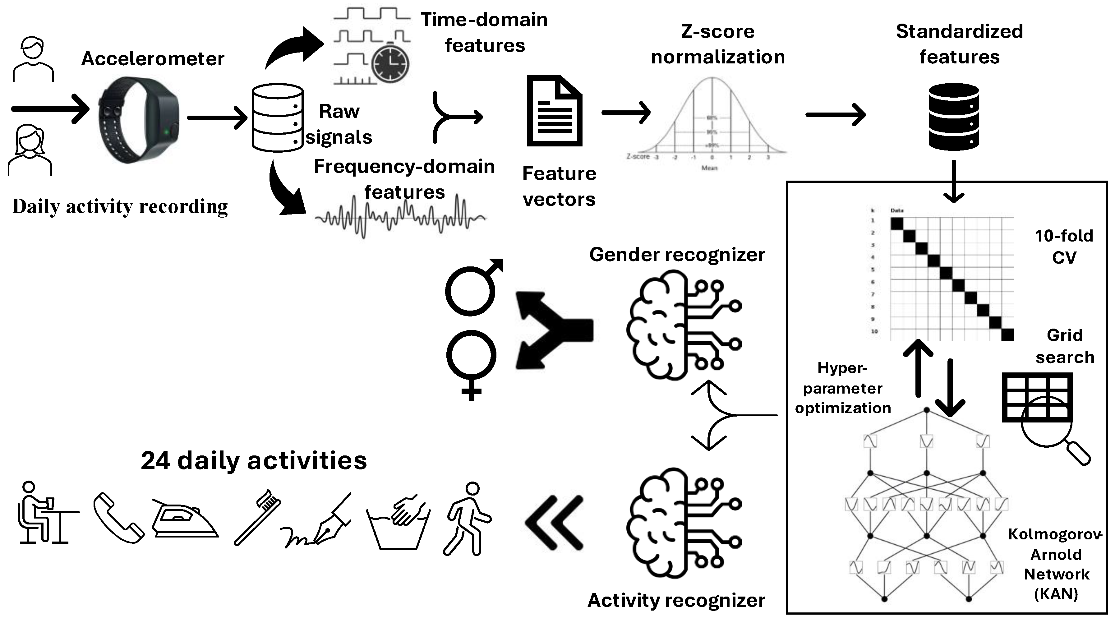
Figure 2.
Confusion matrix for multi-class HAR.
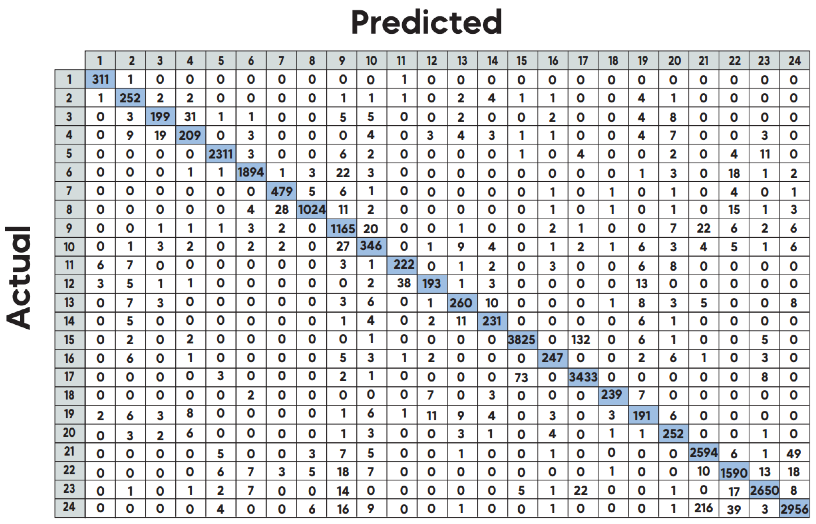
Figure 3.
Confusion matrix for gender recognition.
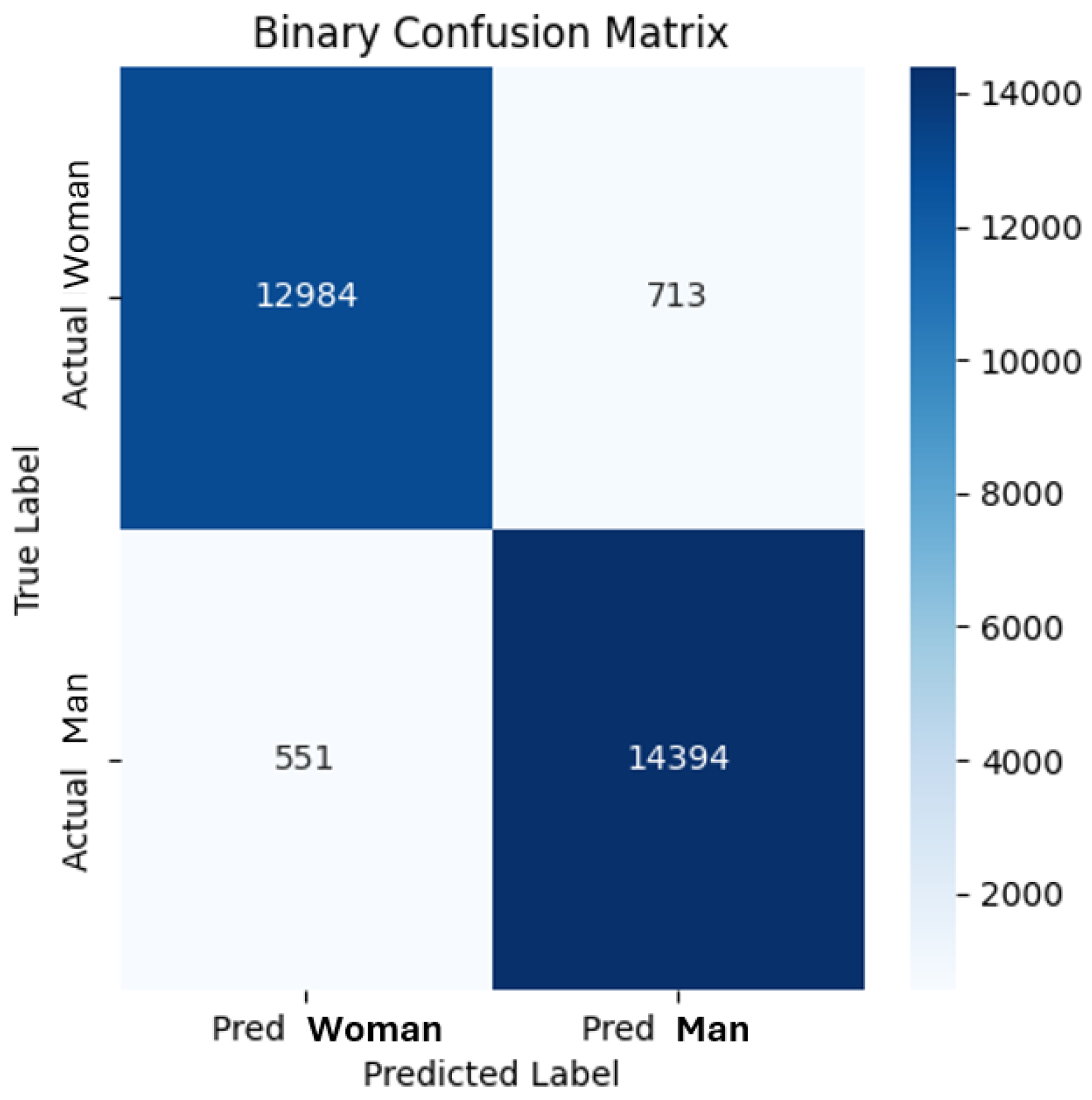
Figure 4.
HR and gender recognition performances on the same dataset.
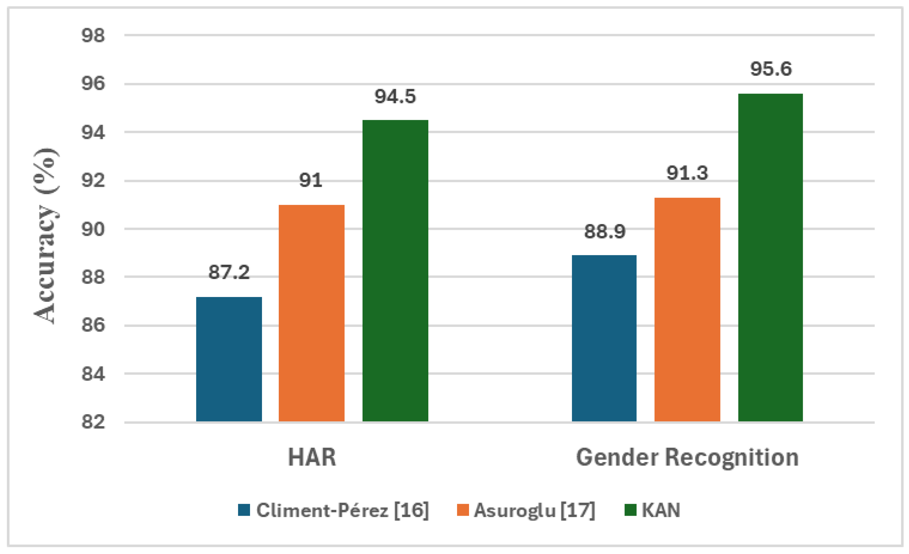
Figure 5.
Relation between number of samples and sensitivity in one-versus-all classification.
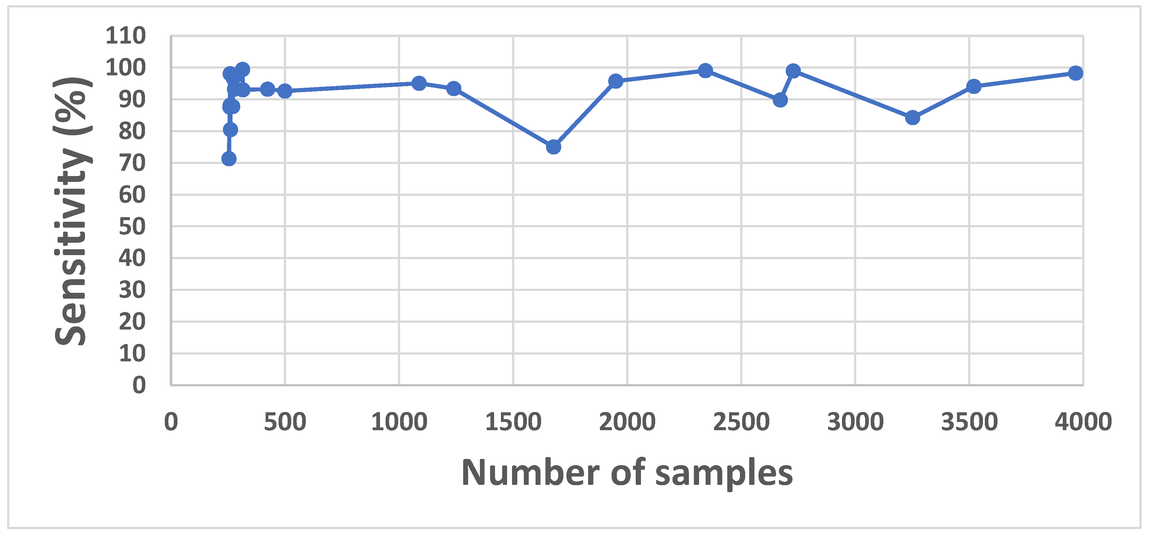

Table 1.
Distribution of samples according to activities.
| Class Label | Activity | Number of Samples |
|---|---|---|
| 1 | Blowing nose | 313 |
| 2 | Brushing hair | 273 |
| 3 | Brushing teeth | 261 |
| 4 | Drinking water | 270 |
| 5 | Dusting | 2344 |
| 6 | Eating meal | 1950 |
| 7 | Taking off glasses | 499 |
| 8 | Putting on glasses | 1088 |
| 9 | Ironing | 1240 |
| 10 | Taking off jacket | 424 |
| 11 | Putting on jacket | 259 |
| 12 | Typing on keyboard | 260 |
| 13 | Opening bottle | 315 |
| 14 | Opening a box | 261 |
| 15 | Making a phone call | 3967 |
| 16 | Saluting | 277 |
| 17 | Taking off a shoe | 3520 |
| 18 | Putting on a shoe | 258 |
| 19 | Sitting down | 254 |
| 20 | Sneezing/coughing | 278 |
| 21 | Standing up | 2672 |
| 22 | Washing dishes | 1678 |
| 23 | Washing hands | 2729 |
| 24 | Writing | 3252 |
| Total: 28642 | ||
Table 2.
Hyper-parameters.
| Hyper-Parameter | Range |
|---|---|
| Hidden layers | Multi-class HAR |
| [62,32,64,128,24] [62,64,128,256,24] [62,128,256,512,24], [62,64,32,16,24] | |
| Binary-class gender recognition | |
| [62,32,64,128,1] [62,64,128,256,1] [62,128,256,512,1], [62,64,32,16,1] | |
| Grid size | [3, 5, 7, 9] |
| Learning rate | [0.0001, 0.001, 0.01, 0.0005, 0.005, 0.05, 0.0002, 0,002] |
| Spline order | [2,3,4,5,6,7,8,9] |
| Scale base | [0.5, 1.0, 1.5, 2.0] |
| Scale spline | [1.0, 2.0] |
| Batch size | [16, 32, 64,128] |
| Optimizer | [Adam, SGD, RMSprop] |
Table 3.
Optimized hyper-parameters.
| Optimized hyper-parameters | ||
| Hyper-parameter | HAR | Gender Recognition |
| Hidden layers | [62, 64, 32, 16, 24] | [62, 128, 64, 32, 1] |
| Grid size | 7 | 7 |
| Learning rate | 0.0001 | 0.0005 |
| Spline order | 7 | 3 |
| Scale base | 1.0 | 1.0 |
| Scale spline | 1.0 | 1.0 |
| Batch size | 32 | 32 |
| Optimizer | Adam | Adam |
Table 4.
Multi-class classification results for HAR.
| Model | Acc (%) | Prec (%) | Sn (%) | Sp (%) | MCC | F1 score | AUC |
|---|---|---|---|---|---|---|---|
| kNN [17] | 88.9 | 88.7 | 88.9 | 99.3 | 0.88 | 0.89 | NR |
| NB [17] | 47.6 | 52 | 47.6 | 96 | 0.44 | 0.5 | NR |
| DT [17] | 71.7 | 71.7 | 71.7 | 98.1 | 0.7 | 0.72 | NR |
| MLP [17] | 74.2 | 74.1 | 74.2 | 98.1 | 0.72 | 0.74 | NR |
| SVM [17] | 69.2 | 68.9 | 69.2 | 97.4 | 0.67 | 0.69 | NR |
| LMT [17] | 73.3 | 73.2 | 73.3 | 97.9 | 0.71 | 0.73 | NR |
| RF [16] | 87.2 | NR | NR | NR | NR | NR | NR |
| LWRF [17] | 91 | 90.9 | 91 | 99.5 | 0.91 | 0.91 | NR |
| Proposed method | 94.5 | 94.6 | 94.5 | 99.7 | 0.94 | 0.95 | 0.97 |
Table 5.
Gender recognition results.
| Model | Acc (%) | Prec (%) | Sn (%) | Sp (%) | MCC | F1 score | AUC |
|---|---|---|---|---|---|---|---|
| kNN [17] | 89.9 | 89.9 | 89.9 | 89.9 | 0.79 | 0.79 | NR |
| NB [17] | 54.8 | 54.6 | 54.8 | 53.3 | 0.09 | 0.55 | NR |
| DT [17] | 73.9 | 73.9 | 73.9 | 73.8 | 0.48 | 0.74 | NR |
| MLP [17] | 65.7 | 65.8 | 65.7 | 65.7 | 0.31 | 0.66 | NR |
| SVM [17] | 59.8 | 59.7 | 59.8 | 59.5 | 0.19 | 0.6 | NR |
| LMT [17] | 75.7 | 75.7 | 75.7 | 75.6 | 0.51 | 0.76 | NR |
| RF [16] | 88.9 | NR | NR | NR | NR | NR | NR |
| LWRF [17] | 91.3 | 91.3 | 91.4 | 91.2 | 0.83 | 0.91 | NR |
| Proposed method | 95.6 | 95.3 | 96.3 | 94.8 | 0.91 | 0.96 | 0.99 |
Table 6.
Accuracy (%) comparison for most confused activities.
| Daily Activity | Our Study | Asuroglu [17] | Climent-Pérez [16] |
|---|---|---|---|
| Putting on a shoe | 93 | 73 | 77 |
| Taking off a shoe | 98 | 97 | 55 |
| Opening a bottle | 83 | 63 | 47 |
| Opening a box | 89 | 69 | 41 |
| Putting on glasses | 94 | 90 | 60 |
| Taking off glasses | 96 | 88 | 50 |
| Standing up | 97 | 95 | 68 |
| Sitting down | 75 | 35 | 58 |
| Making a phone call | 96 | 98 | 52 |
| Sneezing/coughing | 91 | 57 | 33 |
| Blowing nose | 99 | 90 | 56 |
Table 7.
One-versus-all classification results with z-score normalization and w/o normalization.
| Activity vs. All | Acc (%) | Prec (%) | Sn (%) | Sp (%) | MCC | F1 score | AUC |
|---|---|---|---|---|---|---|---|
| Blowing nose | 99.8 | 91.3 | 90.4 | 99.9 | 0.908 | 0.909 | 0.999 |
| 99.9 | 99.7 | 99.4 | 99.9 | 0.995 | 0.995 | 0.999 | |
| Brushing hair | 99.4 | 93.5 | 36.6 | 99.9 | 0.583 | 0.526 | 0.988 |
| 99.8 | 85.4 | 96.7 | 99.8 | 0.908 | 0.907 | 0.999 | |
| Brushing teeth | 99.2 | 60.2 | 21.5 | 99.9 | 0.356 | 0.316 | 0.989 |
| 99.8 | 91.3 | 80.5 | 99.9 | 0.856 | 0.855 | 0.999 | |
| Drinking water | 99.1 | 55.8 | 10.7 | 99.9 | 0.242 | 0.18 | 0.987 |
| 99.8 | 91.9 | 87.8 | 99.9 | 0.897 | 0.898 | 0.999 | |
| Dusting | 98.8 | 94.2 | 90.7 | 99.5 | 0.918 | 0.925 | 0.996 |
| 99.7 | 97.9 | 99.0 | 99.8 | 0.983 | 0.984 | 0.999 | |
| Eating meal | 98.0 | 93.2 | 75.6 | 99.6 | 0.83 | 0.835 | 0.989 |
| 99.3 | 94.4 | 95.7 | 99.6 | 0.947 | 0.951 | 0.997 | |
| Taking off glasses | 99.2 | 74.7 | 82.2 | 99.5 | 0.779 | 0.782 | 0.996 |
| 99.6 | 87.0 | 92.6 | 99.8 | 0.896 | 0.897 | 0.999 | |
| Putting on glasses | 98.2 | 84.7 | 65.0 | 99.5 | 0.733 | 0.735 | 0.991 |
| 99.4 | 88.9 | 95.0 | 99.5 | 0.915 | 0.918 | 0.999 | |
| Ironing | 97.0 | 86.1 | 36.5 | 99.7 | 0.55 | 0.513 | 0.981 |
| 99.0 | 85.0 | 93.4 | 99.3 | 0.886 | 0.89 | 0.996 | |
| Taking off jacket | 98.6 | 81.0 | 8.01 | 99.9 | 0.252 | 0.146 | 0.969 |
| 99.3 | 70.3 | 93.2 | 99.4 | 0.806 | 0.801 | 0.998 | |
| Putting on jacket | 99.4 | 84.2 | 43.2 | 99.9 | 0.601 | 0.571 | 0.992 |
| 99.9 | 88.8 | 98.1 | 99.9 | 0.933 | 0.932 | 0.999 | |
| Typing on keyboard | 99.3 | 79.4 | 31.2 | 99.9 | 0.495 | 0.448 | 0.991 |
| 99.9 | 97.4 | 88.1 | 99.9 | 0.926 | 0.925 | 0.999 | |
| Opening bottle | 99.1 | 63.0 | 54.6 | 99.6 | 0.582 | 0.585 | 0.991 |
| 99.9 | 94.5 | 93.0 | 99.9 | 0.937 | 0.938 | 0.999 | |
| Opening a box | 99.4 | 64.7 | 64.0 | 99.7 | 0.640 | 0.644 | 0.994 |
| 99.8 | 95.0 | 88.1 | 99.9 | 0.914 | 0.915 | 0.999 | |
| Making a phone call | 97.4 | 87.6 | 94.6 | 97.8 | 0.895 | 0.91 | 0.995 |
| 98.7 | 92.3 | 98.3 | 98.7 | 0.945 | 0.952 | 0.999 | |
| Saluting | 99.4 | 78.8 | 48.4 | 99.9 | 0.615 | 0.6 | 0.991 |
| 99.9 | 91.2 | 97.1 | 99.9 | 0.94 | 0.941 | 0.999 | |
| Taking off a shoe | 97.2 | 90.5 | 86.7 | 98.7 | 0.87 | 0.885 | 0.992 |
| 99.1 | 98.1 | 94.1 | 99.7 | 0.955 | 0.961 | 0.999 | |
| Putting on a shoe | 99.6 | 84.9 | 71.7 | 99.9 | 0.778 | 0.777 | 0.997 |
| 99.9 | 100.0 | 87.6 | 100.0 | 0.935 | 0.934 | 0.999 | |
| Sitting down | 99.2 | 67.3 | 13.8 | 99.9 | 0.302 | 0.229 | 0.982 |
| 99.7 | 96.8 | 71.3 | 99.9 | 0.829 | 0.821 | 0.999 | |
| Sneezing/coughing | 99.3 | 79.9 | 41.4 | 99.9 | 0.572 | 0.545 | 0.991 |
| 99.8 | 89.9 | 93.2 | 99.9 | 0.914 | 0.915 | 0.999 | |
| Standing up | 96.2 | 89.0 | 67.9 | 99.1 | 0.758 | 0.77 | 0.988 |
| 98.6 | 94.9 | 89.8 | 99.5 | 0.915 | 0.923 | 0.997 | |
| Washing dishes | 97.2 | 86.1 | 61.3 | 99.4 | 0.713 | 0.716 | 0.98 |
| 98.3 | 94.4 | 75.0 | 99.7 | 0.833 | 0.835 | 0.992 | |
| Washing hands | 97.4 | 90.7 | 81.4 | 99.1 | 0.845 | 0.858 | 0.991 |
| 99.4 | 95.4 | 98.9 | 99.5 | 0.968 | 0.971 | 0.999 | |
| Writing | 94.7 | 76.7 | 76.6 | 97.0 | 0.736 | 0.766 | 0.976 |
| 97.6 | 93.7 | 84.3 | 99.3 | 0.876 | 0.888 | 0.994 |
Table 8.
Performance values w/o z-score normalization.
| Task | Acc (%) | Prec (%) | Sn (%) | Sp (%) | MCC | F1 score | AUC |
|---|---|---|---|---|---|---|---|
| HAR | 78.1 | 77.8 | 78.1 | 100.0 | 0.761 | 0.777 | 0.816 |
| Gender recognition | 77.1 | 74.4 | 68.1 | 74.4 | 0.425 | 0.711 | 0.789 |
Table 9.
HAR performance comparison with deep learning architectures.
| Architecture | Acc (%) | Prec (%) | Sn (%) | Sp (%) | MCC | F1 score | AUC |
|---|---|---|---|---|---|---|---|
| BiLSTM | 80.8 | 80.7 | 80.8 | 98.7 | 0.790 | 0.808 | 0.989 |
| CNN | 94.2 | 94.5 | 94.2 | 99.7 | 0.940 | 0.940 | 0.940 |
| GRU | 79.9 | 79.8 | 79.9 | 98.7 | 0.781 | 0.798 | 0.987 |
| LSTM | 84.3 | 83.4 | 84.3 | 95.2 | 0.829 | 0.836 | 0.976 |
| RNN | 87.3 | 87.5 | 87.3 | 95.0 | 0.861 | 0.872 | 0.996 |
| Proposed method | 94.5 | 94.6 | 94.5 | 99.7 | 0.940 | 0.950 | 0.97 |
Table 10.
Gender recognition performance comparison with deep learning architectures.
| Architecture | Acc (%) | Prec (%) | Sn (%) | Sp (%) | MCC | F1 score | AUC |
|---|---|---|---|---|---|---|---|
| BiLSTM | 68.8 | 69.9 | 70.7 | 66.8 | 0.375 | 0.703 | 0.688 |
| CNN | 82.8 | 83.7 | 83.1 | 82.4 | 0.655 | 0.834 | 0.827 |
| GRU | 73.8 | 75.9 | 73.1 | 74.7 | 0.477 | 0.744 | 0847 |
| LSTM | 76.9 | 76.1 | 75.4 | 78.3 | 0.537 | 0.757 | 0.861 |
| RNN | 83.8 | 83.1 | 83.8 | 84.5 | 0.676 | 0.831 | 0.925 |
| Proposed method | 95.6 | 95.3 | 96.3 | 94.8 | 0.91 | 0.96 | 0.99 |
Table 11.
Statistical significance comparison with deep learning architectures for HAR.
| KAN vs. Architecture | Chi-square statistic | p-value |
|---|---|---|
| BiLSTM | 3420.594 | 0.000 |
| CNN | 865.919 | 0.000 |
| GRU | 3699.303 | 0.000 |
| LSTM | 3066.98 | 0.000 |
| RNN | 1822.349 | 0.000 |
Table 12.
Statistical significance comparison with deep learning architectures for gender recognition
Table 12.
Statistical significance comparison with deep learning architectures for gender recognition
| KAN vs. Architecture | Chi-square statistic | p-value |
|---|---|---|
| BiLSTM | 7025.721 | 0.000 |
| CNN | 2453.494 | 0.000 |
| GRU | 5266.163 | 0.000 |
| LSTM | 4381.682 | 0.000 |
| RNN | 2288.968 | 0.000 |
Disclaimer/Publisher’s Note: The statements, opinions and data contained in all publications are solely those of the individual author(s) and contributor(s) and not of MDPI and/or the editor(s). MDPI and/or the editor(s) disclaim responsibility for any injury to people or property resulting from any ideas, methods, instructions or products referred to in the content. |
© 2024 by the authors. Licensee MDPI, Basel, Switzerland. This article is an open access article distributed under the terms and conditions of the Creative Commons Attribution (CC BY) license (http://creativecommons.org/licenses/by/4.0/).
Copyright: This open access article is published under a Creative Commons CC BY 4.0 license, which permit the free download, distribution, and reuse, provided that the author and preprint are cited in any reuse.


