Section 1. Introduction
The study of dynamical systems, which describes how the state of a system evolves over time under given rules, is fundamental to understanding complex behaviors in various scientific and engineering fields. A crucial aspect of analyzing these systems is determining how they behave near equilibrium points—states at which the system does not change unless perturbed. While the direct analysis of nonlinear dynamical systems can be complex due to their sensitivity to initial conditions and parameters, linearization provides a powerful tool for simplifying this analysis. The Hartman-Grobman Theorem, introduced independently by Philip Hartman and Lev Grobman in the late 1950s (Hartman, 1960; Grobman, 1959), serves as a foundational result in this regard, particularly near hyperbolic equilibria.
The theorem asserts that near a hyperbolic equilibrium point, the behavior of a nonlinear dynamical system can be approximated by its linearized form, allowing for the qualitative study of the system’s dynamics using simpler linear methods. To fully appreciate the implications and applications of the Hartman-Grobman Theorem, it is essential to understand several foundational concepts, which will be introduced and developed in this section.
Section 1.1. Proof of the Hartman-Grobman Theorem
The Hartman-Grobman Theorem states that near a hyperbolic equilibrium point, a nonlinear dynamical system is topologically conjugate to its linearization. Here, we will present the proof in a stepwise, didactic manner with clear explanations of the equations.
Restatement of the Theorem
Let
be a dynamical system with
, where
is continuously differentiable (
) near an equilibrium point
. If the equilibrium point
is hyperbolic, meaning that the Jacobian matrix
has no eigenvalues with zero real parts, then there exists a homeomorphism
(with
and
neighborhoods of
and 0 , respectively) such that the nonlinear system:
is topologically conjugated to its linearized system:
where
preserves the qualitative structure of trajectories.
Step 1: Setting up the Problem
The system under consideration is:
We assume that
is continuously differentiable, and
is an equilibrium point, i.e.,
. Let
be shifted to the origin for simplicity by defining a new variable
. Then the system becomes:
Near
, we linearize
using its first-order Taylor expansion:
where
is the Jacobian matrix of
at 0, and
is a nonlinear remainder term that satisfies:
Thus, the system becomes:
Our goal is to show that this nonlinear system is topologically conjugated to its linearized counterpart . (7)
Step 2: Properties of the Linearized System
The linear system:
has solutions of the form:
where
is the matrix exponential of
, and
is the initial condition.Since
is hyperbolic (by assumption), the eigenvalues of
have nonzero real parts.
This means the space can be decomposed into two invariant subspaces:
Stable subspace, corresponding to eigenvalues with negative real parts.
Unstable subspace, corresponding to eigenvalues with positive real parts.
Any trajectoryof the linearized system will exhibit exponential decay in the stable directions and exponential growth in the unstable directions:
Step 3: Constructing the Homeomorphism
To prove topological conjugacy, we construct a homeomorphism that maps solutions of the nonlinear system to solutions of the linearized system . The strategy is to "straighten" the nonlinear flow using a carefully defined map .
Define the map
by:
where
is a correction function that ensures
maps trajectories of the nonlinear system to those of the linearized system. The function
must satisfy:
, ensuring .
is small near , i.e., vanishes as .
The conjugacy condition holds:
where
is a solution of the nonlinear system.Substituting
into the conjugacy condition, we get:
The left-hand side is:
and from the nonlinear system
, we substitute for
:
The goal now is to solve for , ensuring it is small and smooth near .
Step 4: Existence of the Homeomorphism
The solution for
can be constructed using a fixed-point argument. Specifically, under the hyperbolicity assumption, the operator
defined by:
has a unique solution
that is small near
. By applying the Banach Fixed-Point Theorem in an appropriate function space, it can be shown that such an
exists and satisfies the required smoothness and smallness conditions (Perko, 2013).
Thus, the map
is a homeomorphism, and the conjugacy condition:
is satisfied.
Step 5: Conclusion
Since
is a homeomorphism, the nonlinear system:
is topologically conjugated to its linearized system:
This completes the proof of the Hartman-Grobman Theorem.
Section 1.2. Dynamical Systems
A dynamical system can be defined formally as a system in which a function describes the time dependence of a point in a geometrical space. Mathematically, it is often represented as:
This definition implies that if the system starts at , it remains at indefinitely, representing a constant or steady state of the system. Determining the nature of these points is crucial for understanding the long-term behavior of the system.
Section 1.2.1. Linearization
To analyze the behavior of a system near an equilibrium point
, we often linearize the function
around
. The linearization involves approximating
by its first-order Taylor expansion, leading to:
where
denotes the Jacobian matrix of
at
. This matrix
is crucial as it simplifies the nonlinear system to a linear one, which is easier to analyze.
Section 1.2.2. Hyperbolicity
A point is termed hyperbolic if none of the eigenvalues of the Jacobian matrix at have zero real parts. The significance of this condition lies in the behavior it predicts:
Eigenvalues with negative real parts indicate stability (trajectories converge to ).
Eigenvalues with positive real parts indicate instability (trajectories diverge from ).
The absence of eigenvalues with zero real parts ensures that the system's behavior near is welldefined and predictable, thus satisfying the conditions for the application of the Hartman-Grobman Theorem.
Section 1.3. Topological Conjugacy
Finally, the concept of topological conjugacy provides the framework within which the linear and nonlinear systems are compared. Two systems are topologically conjugate if there exists a homeomorphism
that maps trajectories of the nonlinear system to those of the linear system while preserving their qualitative structure:
where
and
represent the flows of the nonlinear and linear systems, respectively.
This introduction sets the stage for a deeper exploration of the theorem's proof, implications, and applications, demonstrating how the linear approximation facilitated by the Hartman-Grobman Theorem allows for a nuanced understanding of dynamical systems near critical points. Through the use of real-world examples and further theoretical development, we will see how this theorem provides a bridge between complex nonlinear behavior and more manageable linear dynamics.
Section 2. Methodology
In order to rigorously examine the applicability of the Hartman-Grobman Theorem to a given dynamical system, we must follow a systematic approach. This section outlines the methodology employed to determine whether the theorem can be applied to analyze the behavior near equilibrium points and how we can verify the conditions of topological conjugacy between the nonlinear system and its linear approximation.
Section 2.1. Identifying and Analyzing Equilibrium Points
The first step in applying the Hartman-Grobman Theorem is identifying equilibrium points of the dynamical system described by:
where
is the state vector and
is a continuously differentiable function governing the system dynamics. An equilibrium point
satisfies:
Determining involves solving the equation, which may require numerical methods if an analytical solution is not feasible.
2. Linearization at Equilibrium Points
Once an equilibrium point
is identified, the next step is to linearize the system at this point. The linearized form around
is given by the first-order Taylor expansion:
where
is the Jacobian matrix evaluated at the equilibrium point. The elements of
are defined as:
This matrix encapsulates the system's local behavior near and is critical for further analysis.
3. Assessing Hyperbolicity
The equilibrium point
must be hyperbolic for the Hartman-Grobman Theorem to apply. This requires that the eigenvalues
of the Jacobian matrix
do not have zero real parts:
Determining the eigenvalues of provides insight into the stability of and indicates whether trajectories near this point converge or diverge.
4. Verifying Topological Conjugacy
Topological conjugacy between the nonlinear system and its linearization is central to the application of the Hartman-Grobman Theorem. This is verified if there exists a homeomorphism
such that:
Here, represents the flow of the nonlinear system , and is the flow of the linear system . Establishing this relationship typically involves constructing explicitly or proving its existence under the theorem's assumptions.
5. Application to Specific Examples
The final step involves applying the methodology to specific examples to illustrate the theorem's practical implications. For each example, we will:
Calculate the Jacobian matrix at identified equilibrium points.
Assess the eigenvalues to confirm hyperbolicity.
Discuss potential forms for the homeomorphism and how it relates the dynamics of the nonlinear system to its linearization.
By methodically following these steps, we can utilize the Hartman-Grobman Theorem to gain qualitative insights into the dynamics of nonlinear systems near hyperbolic equilibrium points. This methodology not only validates the theoretical aspects but also enhances our understanding through practical application to diverse dynamical systems.
Section 2.2 Practical Application: Population Dynamics Model
A practical application of the Hartman-Grobman Theorem can be seen in ecological models, particularly in understanding the dynamics of populations under certain biological assumptions. One such example is the logistic growth model, which captures how a population evolves over time, taking into account the natural limitations of the environment such as carrying capacity.
-
1.
The Logistic Growth Model
The logistic growth equation for a population is given by:
where:
represents the population size.
is the intrinsic growth rate of the population.
is the carrying capacity of the environment, the maximum population size that the environment can sustain indefinitely.
-
2.
Equilibrium Points
The equilibrium points occur where the growth rate
equals zero. Setting equation (11) to zero, we find:
This yields two equilibrium points:
-
3.
Linearization at Equilibrium Points
We now linearize the logistic model at each equilibrium point. The Jacobian matrix
for this model, which is a scalar in this case since
is a one-dimensional variable, is given by the derivative of the right-hand side of equation (11):
-
4.
Evaluating Jacobian at Equilibrium Points
Assessing Hyperbolicity
Both equilibrium points are hyperbolic since the eigenvalue at each point does not have a zero real part:
for indicates instability (positive eigenvalue, population grows if slightly above zero).
for indicates stability (negative eigenvalue, population returns to if perturbed).
Section 2.3. Implications of the Hartman-Grobman Theorem
The Hartman-Grobman Theorem tells us that the behavior of the nonlinear logistic model near these equilibrium points can be approximated by its linearizations. Specifically:
Near , the linear approximation suggests exponential growth away from extinction if is initially positive.
Near , the linear approximation indicates exponential decay back to if the population is perturbed.
This application of the Hartman-Grobman Theorem enables ecologists to predict and understand the outcomes of small perturbations to a population near critical thresholds, providing crucial insights into the resilience and stability of ecological systems under various conditions.
Section 2.4. Understanding Lipschitz Continuity in the Context of the Logistic Growth Model
Lipschitz continuity is an important mathematical concept in the analysis of differential equations, including those used in dynamical systems like the logistic growth model. This property plays a vital role in ensuring the solutions to these equations behave well, particularly in the context of the Hartman-Grobman Theorem.
-
1.
Definition of Lipschitz Continuity
A function
is said to be Lipschitz continuous on a domain
if there exists a constant
such that:
where
denotes a norm on
. The constant
is called the Lipschitz constant and provides a measure of how sensitive the function
is to changes in its input.
-
2.
Lipschitz Continuity in the Logistic Growth Model
In the logistic growth model described by:
we can assess the Lipschitz continuity of the function
over a domain such as
or
. By computing the derivative
and examining its boundedness, we can establish the Lipschitz condition.
-
3.
Derivative and Boundedness
The derivative of
with respect to
is:
The maximum value of
over the domain will give us the Lipschitz constant
. The derivative achieves its extreme values at the endpoints of the interval
:
Thus, the function is Lipschitz continuous on with a Lipschitz constant . (38)
4. Implications of Lipschitz Continuity
Lipschitz continuity ofimplies that the logistic growth model has well-behaved solutions in terms of stability and convergence properties. Specifically, it ensures that the solutions to the differential equation are unique and depend continuously on the initial conditions within the domain whereis Lipschitz continuous. This is crucial for applying the Hartman-Grobman Theorem since it relies on the system being well-posed to approximate the nonlinear dynamics by the linearized dynamics effectively.
By ensuring Lipschitz continuity, we also establish a groundwork for further numerical analysis and simulations, which can be critical for applying theoretical results to practical scenarios in population dynamics and other fields of study.
In summary, Lipschitz continuity in the logistic growth model not only aids in validating the conditions under which the Hartman-Grobman Theorem applies but also provides assurances regarding the behavior of the model under small perturbations, contributing to a robust understanding of the system's dynamics near equilibrium points.
Section 2.5. Applications
Let's analyse two practical examples where the Hartman-Grobman Theorem can be applied. We will focus on two types of dynamical systems: the logistic growth model and a simple pendulum under small angle approximation. For both examples, we'll code the systems in Python, simulate their behavior, and plot their respective graphs to visualize the dynamics near the equilibrium points.
Example 1: Logistic Growth Model
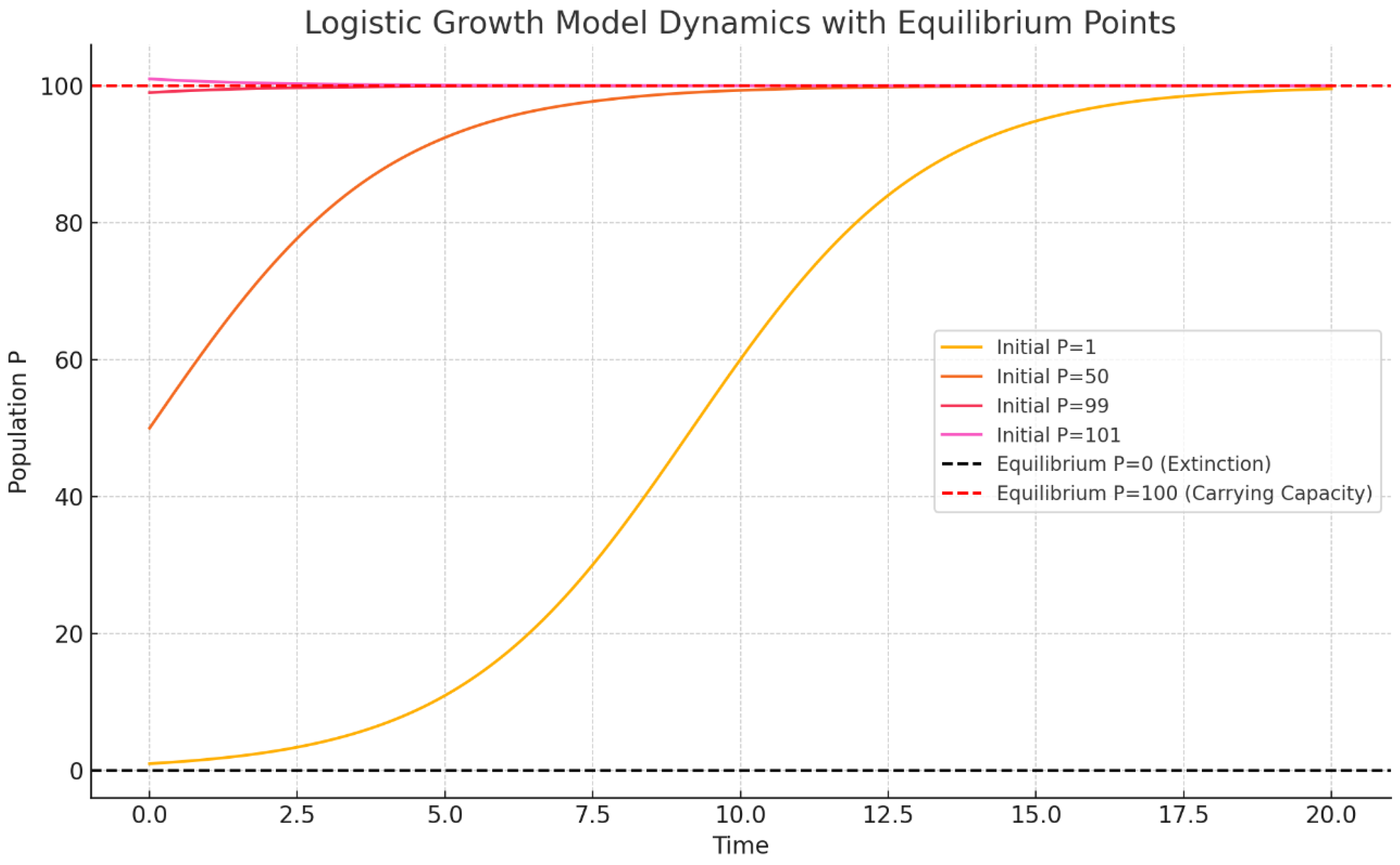
As previously discussed, the logistic growth model describes the population dynamics where the population size is limited by the carrying capacity. We will simulate the behavior of this model near the equilibrium points (extinction) and (carrying capacity).
Chart 1.
Logistic Growth Model Simulation. Note the traced red horizontal line representing the equilibrium at P=100 (K).
Chart 1.
Logistic Growth Model Simulation. Note the traced red horizontal line representing the equilibrium at P=100 (K).
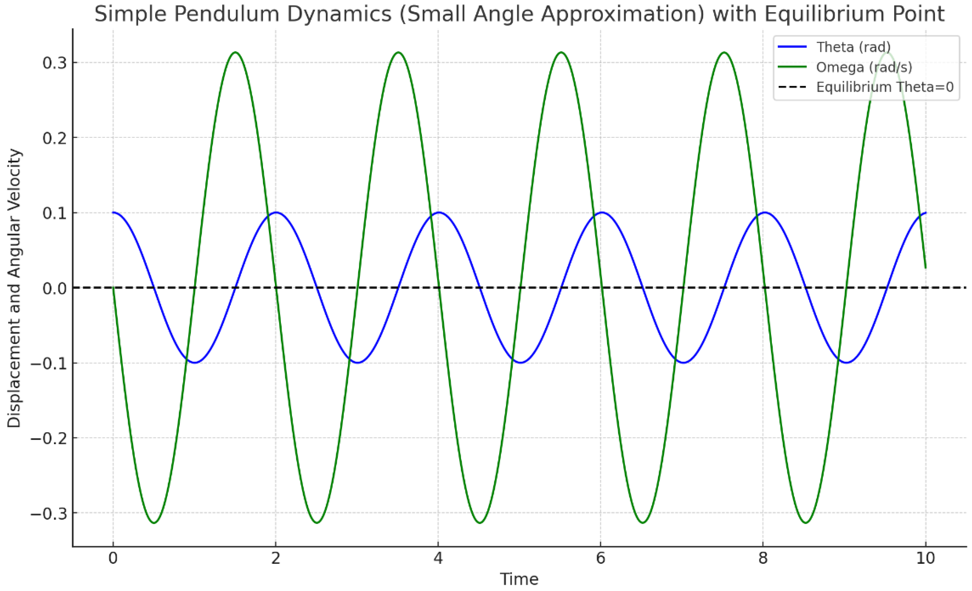
Chart 2.
Simple pendulum dynamics gravitating around point of equilibrium o (Theta).
Chart 2.
Simple pendulum dynamics gravitating around point of equilibrium o (Theta).
- 2.
-
Simple Pendulum (Small Angle Approximation): This graph illustrates the oscillatory behavior of the pendulum under a small initial displacement. The pendulum's angle (theta) and angular velocity (omega) oscillate over time, indicative of the typical harmonic motion expected from the small angle approximation. The model effectively captures the dynamics near the equilibrium (lowest point), showcasing the pendulum returning to its initial state repeatedly due to its stability at this point.
- 3.
Simple Pendulum (Small Angle Approximation): This graph shows the oscillatory motion of the pendulum's angle (theta) and angular velocity (omega). The equilibrium point at , where the pendulum would naturally rest in the absence of any initial movement, is clearly marked with a black dashed line. This helps visualize how the system repeatedly passes through this equilibrium, demonstrating its stability.
These visualizations provide a clearer understanding of how the systems behave near their equilibrium points, highlighting the theoretical concepts in a more visually intuitive manner.
To provide a comprehensive analysis of the simple pendulum dynamics under the small angle approximation, let's study the system's equations, calculate the Jacobian matrix, and establish the Lipschitz continuity constant.
Section 2.5.1.Simple Pendulum Dynamics Equations
For a simple pendulum, the equation of motion derived from Newton's second law for small angular displacements
(where
is assumed to be small enough that
) is:
This second-order differential equation can be transformed into a system of first-order differential equations by introducing
(angular velocity):
This system can be expressed in matrix form as:
Jacobian Matrix
The Jacobian matrix
of the system is derived from the derivatives of the right-hand side functions with respect to
and
. From equations (25) and (26):
Assessing Hyperbolicity
The eigenvalues of the Jacobian matrix
determine the nature of the equilibrium points. The characteristic equation of
is:
Solving this gives the eigenvalues:
These purely imaginary eigenvalues indicate that the system's equilibrium at and is not hyperbolic, and hence, the Hartman-Grobman Theorem does not directly apply. This corresponds to typical harmonic oscillator behavior.
Lipschitz Continuity Constant
The Lipschitz continuity of the system can be investigated by examining the elements of the Jacobian matrix. For the system represented in equation (42), the elements are constants. Hence, the Lipschitz constant
can be determined as the maximum norm of the Jacobian matrix, which in this case, directly corresponds to the maximum absolute value of its elements:
Thus, is the Lipschitz continuity constant, ensuring that the rate of change of the system's state is bounded by this value multiplied by the distance between any two states. This confirms the system's good behavior in terms of solution uniqueness and stability under initial condition variations.
Section 4. Discussion
The Hartman-Grobman Theorem stands as a pivotal result in the qualitative analysis of dynamical systems, providing a rigorous framework for understanding the local behavior of nonlinear systems near hyperbolic equilibrium points. By demonstrating that such systems are topologically conjugated to their linearizations, the theorem allows the study of complex systems through simpler linear models, making it an invaluable tool in mathematics, physics, and engineering. Nevertheless, while its applications are profound and far-reaching, the theorem is not without limitations, particularly when addressing non-hyperbolic equilibria and the qualitative behavior of systems beyond local neighborhoods.
Section 4.1. Strengths of the Hartman-Grobman Theorem
The principal strength of the Hartman-Grobman Theorem lies in its ability to simplify the study of nonlinear systems near hyperbolic equilibrium points. A nonlinear system described by
can be approximated near an equilibrium
through its linearization, where the Jacobian matrix
governs the local dynamics. This result provides a powerful method for identifying stability and qualitative behavior of trajectories using eigenvalues of
(Perko, 2013).
As a result, many practical applications, such as control theory, population dynamics, and fluid mechanics, benefit from the theorem, where approximations near critical points allow for real-world predictions (Guckenheimer & Holmes, 1983).
In population dynamics, the Hartman-Grobman Theorem is widely applied in models such as the logistic growth equation or predator-prey systems. For instance, in the logistic growth model:
the equilibrium points
(extinction) and
(carrying capacity) can be analyzed through their linearized systems. The theorem confirms that near
, the system exhibits local stability, where perturbations return the population to equilibrium. Such analyses are fundamental in ecology and resource management to ensure sustainable population levels (Murray, 2002).
In mechanical systems, the theorem applies to small oscillations, such as in the simple pendulum under small angle approximation. Linearizing the pendulum's nonlinear dynamics near its stable equilibrium (lowest point) reveals harmonic motion governed by:
The Hartman-Grobman Theorem ensures that the local behavior of the nonlinear pendulum near equilibrium matches that of the linearized system, validating the use of simple harmonic motion equations. This is particularly relevant in engineering applications, such as the design of oscillators, clocks, and vibration absorbers (Strogatz, 2018).
In electrical engineering, the theorem is successfully applied to nonlinear circuit analysis, where small-signal approximations near equilibrium points allow the behavior of circuits with diodes, transistors, or other nonlinear components to be analyzed using linear tools. For example, the behavior of a diode-based rectifier circuit near a steady-state voltage can be approximated using its Jacobian matrix, greatly simplifying the design and stability analysis of such systems (Khalil, 2002).
Another example arises in economics, where nonlinear models such as the Solow growth model or predator-prey-inspired business cycle models exhibit equilibria that can be studied using the Hartman-Grobman Theorem. Linearized approximations near steady states allow policymakers and economists to predict economic recovery rates and assess the stability of growth trajectories (Arnold 1998).Another strength of the Hartman-Grobman Thenrem is its generality: it applies to any system where the Jacobian at the equilibrium point has no eigenvalues with zero real parts. This condition ensures hyperbolicity, and thus robustness to small perturbations, which is a key property in fields such as structural mechanics and robotics (Khalil, 2002). By preserving the topological structure of trajectories through homeomorphisms, the theorem ensures that the qualitative nature of the nonlinear system can be captured effectively by its linear counterpart.
Section 4.2. Limitations of the Hartman-Grobman Theorem
Despite its elegance and utility, the Hartman-Grobman Theorem has inherent limitations that constrain its applicability. First and foremost, the theorem applies only to hyperbolic equilibrium points, i.e., those where the Jacobian matrix A has no eigenvalues with zero real parts. This condition excludes a broad class of systems, including those with center manifolds, which exhibit neutral stability (Carr, 1981). Non-hyperbolic equilibria, common in bifurcation theory and nonlinear oscillations, require more sophisticated tools, such as the center manifold theorem or normal form theory, to analyze their local behavior (Wiggins, 2003).
Furthermore, the theorem’s result is valid only in a local neighborhood of the equilibrium point. While this local analysis provides valuable insights into the dynamics near critical points, it does not extend to the global behavior of nonlinear systems. Many real-world systems, particularly those with nonlinearities far from equilibrium, exhibit behaviors such as chaos, limit cycles, or global bifurcations that cannot be captured by linear approximations (Strogatz, 2018). For example, in the Lorenz system, while linearization near equilibria reveals local stability, the system’s chaotic attractors and nonlinearity in larger domains require numerical simulations and global analysis.
Another significant limitation is the assumption of Lipschitz continuity or differentiability of the nonlinear function f(x). While the theorem holds under these regularity conditions, many systems of practical interest are governed by discontinuous dynamics, as seen in control systems with switching mechanisms or economic models with thresholds (Filippov, 1988). In such cases, the linearization procedure breaks down, and alternative methods like piecewise smooth systems must be applied.
Section 4.3. Practical Considerations and Broader Context
In practical terms, while the Hartman-Grobman Theorem simplifies nonlinear systems through linearization, it must be used with caution when applied to real-world scenarios. The theorem's reliance on eigenvalues assumes precise knowledge of the system parameters, which may not always be feasible in empirical studies. Small inaccuracies in the Jacobian matrix due to measurement errors or model approximations can lead to incorrect predictions of stability (Hale & Koçak, 1991). This sensitivity highlights the need for complementary numerical techniques, such as bifurcation analysis and numerical simulations, to validate theoretical results.
Additionally, the theorem's scope is limited to deterministic systems. In many modern applications, such as climate models and financial systems, stochastic effects play a significant role, and linear approximations must be extended to include noise and uncertainty (Arnold, 1998). Techniques such as stochastic differential equations and Lyapunov exponents are more appropriate in such contexts.
Summary
The Hartman-Grobman Theorem is a cornerstone result in the analysis of dynamical systems, offering a robust framework for approximating nonlinear dynamics near hyperbolic equilibria. Its strengths lie in its generality, simplicity, and applicability to diverse fields, from biology to engineering. However, the theorem's limitations, particularly its restriction to hyperbolic equilibria and local neighborhoods, underscore the need for complementary methods in cases involving non-hyperbolic points or global dynamics. While it remains an essential tool for understanding the qualitative behavior of dynamical systems, it must be applied judiciously and in conjunction with broader analytical and numerical techniques to address the complexities of real-world nonlinear phenomena.
Section 5. Conclusion
The Hartman-Grobman Theorem is a fundamental result in the qualitative theory of dynamical systems, offering a powerful method for analyzing the local behavior of nonlinear systems near hyperbolic equilibrium points. By establishing that such systems are topologically conjugate to their linearized counterparts, the theorem enables a significant simplification in understanding the stability and trajectories of nonlinear systems. Its broad applicability across disciplines, including biology, mechanics, electrical engineering, and economics, highlights its utility in real-world problems where approximations near equilibria yield valuable insights.
However, the theorem’s limitations must be carefully considered. It is constrained to hyperbolic equilibria, where the Jacobian matrix has no eigenvalues with zero real parts, and its validity holds only within local neighborhoods of equilibrium points. These restrictions exclude systems with non-hyperbolic equilibria, global nonlinearities, or discontinuous dynamics, necessitating alternative techniques like center manifold theory, bifurcation analysis, or stochastic models. Furthermore, the sensitivity to model parameters and measurement inaccuracies underscores the importance of complementing theoretical results with numerical simulations to ensure robustness and accuracy.
In conclusion, while the Hartman-Grobman Theorem is an invaluable tool for approximating and analyzing nonlinear systems, its application requires careful consideration of its assumptions and scope. It serves as a foundation upon which more advanced methods can build, facilitating a deeper understanding of the rich and complex behaviors inherent in nonlinear dynamics.
*The Author claims there are no conflicts of interest.
Section 6. Attachment:
Python Code (without indentations):
Code for Logistic Growth Model
import numpy as np
import matplotlib.pyplot as plt
from scipy.integrate import solve_ivp
# Parameters
r = 0.5 # Growth rate
K = 100 # Carrying capacity
# Logistic growth function
def logistic_growth(t, P):
return r * P * (1 - P / K)
# Time span
t = np.linspace(0, 20, 1000)
# Initial conditions near the equilibrium points
initial_conditions = [1, 50, 99, 101] # Slightly above 0, around K/2, just below K, just above K
# Plotting
plt.figure(figsize=(10, 6))
for P0 in initial_conditions:
sol = solve_ivp(logistic_growth, [t.min(), t.max()], [P0], t_eval=t)
plt.plot(sol.t, sol.y[0], label=f'Initial P={P0}')
plt.title('Logistic Growth Model Dynamics')
plt.xlabel('Time')
plt.ylabel('Population P')
plt.legend()
plt.grid(True)
plt.show()
# Parameters
g = 9.81 # Acceleration due to gravity, m/s^2
L = 1 # Length of the pendulum, m
omega = np.sqrt(g / L) # Angular frequency
# Pendulum system (small angle approximation)
def pendulum(t, theta):
return [theta[1], -omega**2 * theta[0]]
# Initial conditions
theta0 = [0.1, 0] # Small initial displacement in radians, no initial angular velocity
# Time span
t = np.linspace(0, 10, 1000)
# Solving the differential equation
sol = solve_ivp(pendulum, [t.min(), t.max()], theta0, t_eval=t)
# Plotting
plt.figure(figsize=(10, 6))
plt.plot(sol.t, sol.y[0], label='Theta (rad)')
plt.plot(sol.t, sol.y[1], label='Omega (rad/s)')
plt.title('Simple Pendulum Dynamics (Small Angle Approximation)')
plt.xlabel('Time')
plt.ylabel('Displacement and Angular Velocity')
plt.legend()
plt.grid(True)
plt.show()
References
- Arnold, L. (1998). Random Dynamical Systems. Springer.
- Carr, J. (1981). Applications of Centre Manifold Theory. Springer-Verlag.
- Filippov, A. F. (1988). Differential Equations with Discontinuous Righthand Sides. Kluwer Academic.
- Guckenheimer, J., & Holmes, P. (1983). Nonlinear Oscillations, Dynamical Systems, and Bifurcations of Vector Fields. Springer-Verlag.
- Hale, J. K., & Koçak, H. (1991). Dynamics and Bifurcations. Springer-Verlag.
- Khalil, H. K. (2002). Nonlinear Systems (3rd ed.). Prentice Hall.
- Murray, J. D. (2002). Mathematical Biology (Vol. 1). Springer-Verlag.
- Perko, L. (2013). Differential Equations and Dynamical Systems. Springer.
- Strogatz, S. H. (2018). Nonlinear Dynamics and Chaos (2nd ed.). CRC Press.
- Wiggins, S. (2003). Introduction to Applied Nonlinear Dynamical Systems and Chaos. Springer.
|
Disclaimer/Publisher’s Note: The statements, opinions and data contained in all publications are solely those of the individual author(s) and contributor(s) and not of MDPI and/or the editor(s). MDPI and/or the editor(s) disclaim responsibility for any injury to people or property resulting from any ideas, methods, instructions or products referred to in the content. |
© 2024 by the authors. Licensee MDPI, Basel, Switzerland. This article is an open access article distributed under the terms and conditions of the Creative Commons Attribution (CC BY) license (http://creativecommons.org/licenses/by/4.0/).