
Submitted:
24 December 2024
Posted:
25 December 2024
You are already at the latest version
Abstract
Austenitic stainless steel SS316LN is used as the material of construction of vessel and core components of fast breeder reactors, which operate at an elevated temperature of 550 deg. C. For design and integrity analysis using finite element method, material models, such as Johnson-Cook and Ramberg-Osgood, are widely used. However, the temperature-, strain-rate dependent plasticity and damage parameters of these models for this material are not available in literature. Moreover, the method of evaluation of temperature and strain-rate dependent plasticity parameter in literature has some major shortcomings, which have been addressed in this work. In addition, a new optimization based procedure has been developed to evaluate all the nine plasticity and damage parameters, which uses results of combined finite element analysis and experimental data. The procedure has been validated extensively by testing tensile specimens at different temperatures, by testing notched tensile specimens of different notch radii and by carrying out high strain-rate tests using split Hopkinson pressure bar test setup. The parameters of Johnson-Cook material model, evaluated in this work, have been used in finite element analysis to simulate load-displacement behavior and fracture strains of all types of specimens and the results have been compared with experimental data in order to check the accuracy of the parameters. This procedure developed in this work shall help the researchers to adopt such technique for accurate estimation of both plasticity and damage parameters of different types of material models.
Keywords:
Johnson-Cook model
; Plasticity and Damage
; Austenitic stainless steel
; SS316LN
; Notched tensile test
; High temperature test
; Split Hopkinson pressure bar test
; Finite element analysis
1. Introduction
The major components of the reactor assembly in the Prototype Fast Breeder Reactor (PFBR), such as the grid plate, core support structure, main vessel, inner vessel, and intermediate heat exchanger, are made of austenitic stainless steel grade 316LN (SS316LN) [1]. These components are exposed to high temperatures and are submerged in liquid sodium metal. PFBR uses hot liquid sodium metal (500°C-550°C) as a coolant, which subjects materials to high thermal stresses due to sodium's high convective heat transfer coefficient. SS316LN is the preferred structural material because it is a low-carbon steel grade that avoids sensitization during welding, preventing stress corrosion cracking in the chloride-rich environments of coastal sites. SS316LN also exhibits excellent mechanical properties, including tensile strength, creep resistance, low-cycle fatigue, creep-fatigue interaction, and high-cycle fatigue strength at both low and high temperatures [2].
For design by analysis, the reactor components are designed using standard codes, which have been developed by American Society of Mechanical Engineers (ASME) and French engineers. Among these codes, the RCC-MR code [3], is a predominant French design code, which is used for design of components of fast breeder reactors. This code provides design curve equations for the stress-strain relationship at various temperatures for SS316LN, however, these are valid up to 1.5% plastic strain only. The design curve expressions as provided in the RCC-MR code are not valid if plastic strain exceeds 1.5%. Higher plastic strains can occur in regions of structure with large geometrical discontinuities, such as shell-nozzle junctions, vessel heads, and T-junctions etc. Typically, design procedure uses the lower-bound stress-strain curve, however, the life or integrity assessment techniques use the median value of stress-strain curve. This indicates that different approaches are needed while carrying out design and safety analysis of the reactor components.
High temperature properties of SS316LN are essential for integrity analysis of reactor components during severe accident scenarios. The postulated Core Disruptive Accident (CDA) is one such accident, which occurs due to melting of nuclear fuel in the reactor core. This can lead to significant rise in the temperature of the coolant and the structural material (of the order of 1000oC). At the elevated temperatures, significant changes in strength and ductility of SS316LN stainless steel occurs. Hence, the properties of the structural materials need to be evaluated at different temperatures and incorporated in an appropriate material constitutive model for finite element analysis in order to demonstrate that the reactor core is safe during CDA and other such postulated severe accidents.
The postulated CDA can also impart shock loads on structural components. For analysis of these scenarios, a rate-dependent material model is essential for structural integrity analysis of reactor assembly components, especially the main vessel. However, the RCC-MR code [3] neither provides rate-dependent stress-strain data nor the parameter of material constitutive models such as those of Johnson-Cook [4]. For thermo-mechanical analysis of structural components, where temperature varies across the thickness of the component, temperature-dependent material stress-strain data, provided in the form of true stress-strain curves, are essential input data for the analysis and it is one of the approaches in finite element analysis. On the other hand, use of temperature and strain-rate-dependent Johnson-Cook model is more elegant as it models both the plastic hardening behavior and softening behavior due to incorporation of damage parameter. It takes care of coupled effect of damage softening, thermal softening and strain hardening and strain rate hardening phenomena on the material deformation behavior.
In this work, the temperature and strain-rate dependent plasticity and damage parameters of Johnson-Cook material model for austenitic grade stainless steel SS316LN is evaluated by following a new procedure, where both experimental data and results of finite element (FE) analysis have been used. The parameters evaluated through this procedure has been validated extensively using data of both smooth and notched tensile specimens at different temperatures. In addition, the parameters of Ramberg-Osgood material model in the range of 25-650oC have been evacuated for SS316LN using an optimization algorithms, which takes into account both experimental data and FE analysis results of smooth as well as notched tensile specimens. The parameters of Ramberg-Osgood material model (i.e., ‘n’ and ‘α’) are popularly used in closed-form solutions and estimation schemes [5,6], such as those provided by electric power research institute (EPRI), USA. These schemes are useful for evaluation of J-integral, crack mouth opening displacement, load-line displacement and other such crack-tip loading parameters, which are essential for integrity analysis of components using fracture mechanics principles.
This paper has been divided into eight sections. After a brief introduction to the problem in Section-1, the relevant literature is discussed in Section-2. The details of material composition, specimen design, experimental procedure, test data and mechanical properties of SS316LN stainless steel at different temperatures have been presented in Section-3. The conventional procedure (as available in literature) and the new algorithm for evaluation of plastic hardening parameters of both Johnson-Cook and Ramberg-Osgood models are provided in Section 4 and Section 5 respectively. The procedure for evaluation of damage parameters of Johnson-Cook material model is presented in Section-6 followed by a discussion and validation of results in Section-7. The paper ends with the concluding remarks in Section-8.
2. Brief Review of Literature on SS316LN, Material Plasticity and Damage Models
Austenitic grade stainless steel SS316LN is used in both fission and fusion type reactors for manufacturing of their components due to its excellent corrison resistance, mechanical and fracture properties at both cryogenic and elevated temperature environment. In international thermonuclear experimental reactor (ITER), SS316LN is used as material of cryogenic jackets and central solenoid [7]. The metallurgical and mechanical properties of two gardes of austenitic stainless steels used as material of conductor jacket of the ITER central solenoid have been presneted in Ref. [7]. The tensile test data of SS 316LN jacket material are presented in Ref. [8]. The effects of cryo-rolling and other methods of plastic prestraining on change in microstructre, mechanical and fracture properties of SS316LN steel have been studied extensively in litearture [9,10,11,12,13,14,15,16].
The influence of thermo-mechanical processing conditions on mechanical properties of SS316LN steel has been studied and presented in Kvackaj et al. 2020 [17]. Stress corrosion cracking of SS316LN stainless steel in primary water environment of ITER and the ratcheting-induced twinning/de-twinning behavior is studied in Ref. [18] and [19] respectively. Different methods have been employed in litearture to modify and enhance the properties of austenitic grades of stainless steel, such as spray forming [20],surface mechanical attrition treatment [21], and heat-treatment [22,23] etc.
Rcently, many types of novel manufacturing techniques (metal powder injection molding [24], direct energy deposition [25], additive manufacturing [26] etc.) have been developed, which are fast, efficient and are suitable to tailor the mechanical and fracture porperties of asustenitic stainless steel components. A comparative analysis of mechanical properties of SS316L as obtained through conventional and additive manufacturing techniques has been presented in Ref. [27]. A review of processing techniques, microstructure, properties and performance of austenitic grade stainless steels at high temperatures is presented in Ref. [28].
Another important apsect, that is investiaged in litearture, in the study of high temperature deformation behaviour of austenitic grade stainless steel is its microstructure instabilities. Way back in 1972, Weiss and Stickler [29] studied the phase instabilities in the mcirostructure of SS316 grade austenitic stainless steel during its high temperature exposure. Later, several authors [30,31,32,33,34,35] have reported precipitation of different types of intermetallic compounds and brittle phases (e.g., σ, χ, η) in the matrix, espacially when the temperature exceeds 650oC, which can alter the mechanical and fracture properties of these grades of materials.
Studies involving evaluation of tensile and fracture priperties of austenitic grade stainless steel SS316LN are very limited in litearture, especially when the high temperature and rate-dependent mechanical andfracture properties are concerned. However, extensive liteature exist regarding creep [36,37], time-dependent deformation behavior [38] and low cycle fatigue property evaluation [39,40,41], thermal and thermo-mechanical fatigue [42,43,44], multi-axial low cycle fatigue [42,44], , mechanical and thermo-mechanical fatigue crack growth [45,46], effect of strain rate on low cycle fatigue crack growth [47] of the above grade of stainless steel. Constitutive modelling of creep [48], cyclic deformation [49] and hardening behaviour [50] of austenitic grades of stainless steels have also been presented in literature. A modelling technique involving first-principles simulations has been presented by Li et al. [51], which has been used to study evolution of defect structire in the material and its corresponding effects on the mechanical properties of SS316LN stainless steel. The fracture properties of austenitic grades of stainless steel are presented in Ref. [52,53,54,55]. The mechanism of fracture process at cryogenic temperature environment has also been studied for SS316LN laser welded joints in Ref. [55]. Ball idnentation technique has been used by Kumar et al. [56] and Ragavendran et al. [57] to evaluate tensile properties of thermally aged 316LN stainless steel with varying nitrogen content and welded joints respectively. The effect of hydrogen on tensile property and strain rate dependent property of SS316L stainless steel has been studied in Ref. [58,59].
In summary, it can be said that several studies exist in litearture involving creep, low cycle fatigue, fracture properties of different grades of austenitc stainless steels such as SS316L and SS316LN. The liteature involving teperature and strain-rate-dependent properties and corersponding material constitutive models for SS316LN is very limited. Some data, which uses ball indentation tests of thermally-aged SS316LN and its laser-weld joint at room temperature, to evaluate their mechanical properties for grades containing different notrigen content have been presented in Ref. [56,57], however, ball indentation involves compression loading and properties such as fracture strain and ultimate tensile strength can’t be evlaluated dierctly from these tests. Moreover, void growth and coalescence mechanisms, which correspond to damage development in the material are not activated in compressive type ball indentation tests and hence, these types of tests are not relevant for development of design data for SS316LN for its use in design and integrity analysis of reactor components. The objective of this work is to fill this gap in litearture and to develop a Johnson-Cook type generalized temerature and strain-rate-dependent material constitutive model for SS316LN, which can be used for design and integrity analysis using FE method.
3. Material Used in This Work and Other Experimental Details
The material used in this work for carrying out different types of tests is austenitic grade stainless steel SS316LN. As memntioned earlier, this material is used as material of construction of core components and vessels of Indian prototype fast breeder reactor (PFBR) [1]. The chemical composition of the alloy is provided in Table 1. It is a 18Cr-12Ni-3Mo grade austenitic stainless steel with 0.06-0.08% N with Ti and Nb added to prevent extensive chromium depletion due to carbide formation.
For evaluation of mechanical propeties of this alloy in high temperature environment, specimens have been designed and machined from the SS316LN plates and the geometrical details of the specimens have been provided in Figure 1(a). Both smooth and notched tensile specimens have been used in the tests. Notched tensile specimens have been used in odrer to evaluate the damage parameters of Johnson-Cook material model [4], where the effect of stress triaxiality of stress state in the specimen on its fracture strain is evaluated experimentally and through use of FE analysis. The details of Johnson-Cook plastic hardening and damage model and procedure for evaluation of the parametrs shall be discussed in later sections.
It may be noted that the minimum cross-sectional area of both smooth and notched tensile specimens is kept same so that the effect of notch radius on change in fracture strain and the notch-strengthening effect can be studied systematically. Tests have been conducted at different temperatures ranging from room temperature (25oC) to 1000oC, which covers a very wide temperature range, that is suitable for both design and integrity analysis at elevated temperatures during postulated severe accident scenarios. The load-displacement data as obtained from the experiments in the range of 25-1000oC are presented in Figure 1(b). The corersponding engineering and true stress-strain data for the material are presented in Figure 1(c-d). From engineering stress-stain data as presented in Figure 1(c), it may be observed that SS316LN exhibits significant plastic strain hardening for an extended range of plastic stain values ranging from 0.35 to 0.62, which changes with temperatures. After reaching maximum stress (corresponding to ultimate tensile strength UTS), the specimen breaks akmost suddenly with limited extension, which is due to extensive void growth and coalescence in the central high triaxial notched region of the deformed specimen. This is also consistent with observaton in literature data.
However, after temerature reaches and exceeds 700oC, the pre-UTS elongation (measured in terms of strain here) becomes smaller and the post-UTS elongation increases significantly as can be seen from engineering stress-strain data presented in Figure 1(c). The pre-UTS strain reduces monotonically with increase in temperature from 700oC to 1000oC, whereas the post-UTS strain increases. This indicates microstrucrual instability and precipiattion of different types of intermetallic phases in austenitic grades of stainless steel as reported extensively in literature [29,30,31,32,33,34,35]. These phases in the austenitic matrix affects the plastic deformation and hardening behavior and also the fracture behavior as these help in forming of microscopic cracks in the matrix either due to cracing of these brittle phases or decoheson of these phases from the ductile matrix. The competition between precipitation and dissolution of different types of phases also affects the plastic hardening and micro-crack development during high temperature deformation of this material.
The notched tensile specimens (with different notch radii of 0.5 , 1, and 2 mm) have been tested at 25oC and the corresponding load-displacement data have been presented in Figure 2(a). The notched specimens have been designed in such a way that the minimum cross-section (2x2 mm2) of both smooth and notched type tensile specimens are kept same. This shall help in studying the effect of stress triaxiality (which has been induced indirectly by changing value of notch radius) on fracture strain and notch-strengthening behavior. As shown in Figure 2(a), the hardening behavior and peak load incrases significantly for the notched specimens when compared to the smooth specimen, though the minimum cross-section of both types of specimens are same. It can be explained on the basis of development of high stress triaxial condition in the notched region of the notched specimens, which prevents the plastic deformaton.
The details of evauation of stress traixiaty as a function of notch radius shall be discussed later which requires FE analysis. It is known that plastic yielding (based on vin Mises criteria, also known as distortion energy theory) is independent of hydrostatic stress and hence, stress triaxiality. The presence of higher values of riaxial stress field (lesser the notch radius) prevents plastic deformation for same value of applied remote tensile stress (and uniaxial load applied away from nocthed region of the specimen) and hence, the notched specimens requires more load to undergo similar extents of plastic deformation as that of the smooth tensile specimen. This is reflected in the load-displacement results of different types of specimens as presented in Figure 2(a)
Moreover, the fracture displacement (and strain) also reduces with decreasing notch radius and increasing stress triaxiliaty as presented in Figure 2(a) and (b). The peak load-carrying capacity of the noctehd specimens also increases with decreasing notch radius as presneted in Figure 2(a-b), also known as notch-strengthening effect. However, it may be noted that the material true stress-strain curve, as used in material constitutive models in FE analysis, which uses von Mises criteria is independent of stress triaxilaity in the specimen and hence, hence, the notch strengthening is a geometrical phenomena.
Another issue that arises in the evaluation process of fracture strain and stress triaxiality values in notched specimens is that, these values are neither constant for a specimen (with a given geometry and notch radius) nor uniform across the minium cross-sectional area unlike that of a smooth tensile specimen, where the magnitude of stress traixility (defined as ratio of hydrostatic stress to von Mises equivalent stress) is 1/3. These issues have been addresed in this work through use of FE analysis and the details shall be presented in later sections.
The yield strength and UTS of SS316LN at different temperatures have been presented in Figure 2(c-d). It may be noted that the yield strength decreases monotonically with increase in temperature due to softening of the matrix of the material and easy movement of dislocation due to higher thermal activation. The decrease in yield strength and UTS from 25 to 200oC is somehow rapid, followed by a slow decrease in the temperature range of 200-600oC. After 600oC, the UTS decreases rapidly due to onset of instability in the microstruture [29,30,31,32,33,34,35] of the material as discussed earlier.
The decrease in yield strength (YS) is not so rapid as compated to the change in UTS values as YS signifies onset of plastic defromation (or process of initiation of yielding) and hence, the effect of microstructural instabilities becomes significant only at larger magnitudes of plastic deformations and hence, it affects the UTS more. The mechanical property (YS and UTS) as evaluated in this work have also been compared with lower and upper bound data of the same material as presented in French design and safety analysis code RCC-MR [3]. However, RCC-MR doesn’t provide data upto 1000oC as can be seen from Fug. 2(c-d). It can be observed that our data follows the trend of RCC-MR data for the whole temperature range and these are also within the two statistical bounds. After evaluation of temperature-dependent mechanical property and true stress-strain curve for SS316LN, we have used the information to evaluate the parameters of material constitutive models, such as those of Johnson-Cook and Ramberg-Osgood. The process of evaluational of parameters of these models, using conventional procedure has some issues, which have been addressed in the subsequent sections.
4. Conventional Procedure and a New Algorithm for Evaluation of Parameters of Temperature and Strain-Rate-Dependent Material Constitutive Models
For evaluation of plastic strain hardening, strain-rate hardening and thermal softening parameters of SS316LN, Johnson-Cook material model [4] has been used in this work. In this model, von Mises equivalent true stress ‘σ’ is expressed as a function of equivalent plastic strain, true equivalent plastic strain rate , normalized temperature T* or Tnorm as presented in Eq. (1). The differential temperature (i.e., the difference between operating temperature T or Tref) is normalized with respect to the differential value of melting temperature of the material Tm (w.r.t Tref) as presented in Eq. (2) to define normalized paramete T*. The first term in Eq. (1) represents plastic stain hardning term, the second terms refers to the strain-rate hardening term and the last term corresponds to the thermal softening term.
In this work, the reference temperature is taken as 25oC and hence, for room temperature tests, the Johnson-Cook material model can be expressed as given in Eq. (3), where the last term of Eq. (1) becomes unity.
The issue of evaluation of flow stress (also known as true stress) as a function of cumulative plastic defromation, strain rate and temperature and its presentation in a relevant coupled mathematical form (suitable for incorporation in material constitutive models in FE simulations) has been studied extensively in litearture [4,60,61,62].
However, the model proposed by Johnson and Cook [4] has its unique advantages in its simpliciy and ability to model the plastic strain hardening behaviour of a wide class of materials ranging from carbon steel, low-alloy steel, copper, aluminium, stainless steel, magneisum and other engineering materials. Later, the palstic strain hardeing model has been supllemented with a damage model [63] by taking into account of the fracture characteristics of different types of materials when subjected to various magnitudes of strains strain rates, temperatures and hydrostatic pressures (also presented as stress triaxiality).
The model as presented in Eq. (4) expresses equivalent plastic stain at damage (which is a critical value of equivalent plastic strain at which onset of material degradation occurs and the material point subsequently looses its stress carrying capability by reducing the strength in an exponential decay type manner) as a function of stress triaxiality, strain rate and normalzied temperature.
where and are called damage parameters of Johnson-Cook model. The stress triaxiality ( is defined as where and are the hydrostatic (mean) stress and von Mises equivalent stress values respectively. Later, several modifications to the mathematical forms of Johnson-Cook model have been carried out by various researchers [64,65]. Some of these expressions are presented here briefly. A modified form of JC model was presented in Ref. [64] to model the material deformation behaviour during the hot stamping process of B1500HS boron steel. This modification included a power law exponent in the strain-rate-dependent term (i.e., second bracket) and an additional coefficient in the temperature-dependent term (i.e., third bracket) as presented in Eq. (5) below.
Later, Wang et al. [65] modified the plastic strain dependent term (i.e., term in the first bracket) of Eq. (1) and they instead used a quadratic polynomial expression instead of the power law as presented in Eq. (6). In addition, the strain-rate and temperature dependent terms were coupled together and expressed through an exponential function as presented in the third term of Eq. (6).
Zou et al. [66] further modified the plastic strain dependent term of the true stress through a cubic polynomial as presented in Eq. (7), keeping the other two terms similar to those of Ref. [65].
The method of identification of parameters of Johnson-Cook material model as presented through Eqs. (1) and (4) is very challenging as it involves several types of specimen design for the tests, which includes smooth as well as notched tensile specimens, high strain-rate tests, high temperature tests etc.
Moreover, the evaluation of stress triaxility values for different types of notched tensile specimens requires use of complex analysis procedure, which are not trivial for an experimentalist and these also can’t be directly evaluated from experimental measurement as done while evaluating mechanical properties such as YS, UTS and ductility etc. Several works have been reported in literature [65,66,67,68,69,70,71] regarding identification of parameters of Johnson-Cook material model. This damage model has also been used in Ref. [69] to evaluate machinability characteristics of materials.
The model parameters have been evauated using an optimization approach involving fireworks algorithm in Ref. [71]. It can be seen that the procedure for identification of Johnson-Cook model parameters, especially the damage parameters (i.e., d1 to d5) is complex. It needs thorough understanding of the model as regards to its applicability in simulating material deformation behavior at different temperatures and strain rates. In this work, the conventional method for identification of the parameters shall be presented first.
The difficulty of the parameters (as evaluated using the conventional procedure) shall be highlighted by comparing the results of the FE simulation with a wide range of experimental data and a new procedure shall be presented, which is based on minimization of error in simulation of load-displacement behavior of different specimens when compafred with experimental data.
Before proceeding with the discussion regarding evaluation of parameters of Johnson-Cook material model, a schematic explanation of material hardening and softening responses of the material as presented by the above model is presented in Figure 3. This figure represents the variation of true stress in the material point as a function of cumulative equivalent plastic strain. The curve as presented in Figure 3(a) has been divided into two parts, i.e., plastic hardening part represented by Johnson-Cook plasticity model (Eq. 1) and Johnson-Cook damage model (Eq. 4). Once the critical value of equivalent plastic strain for damage as presented in Eq. (4) is reached in the material point during ongoing deformation, damage initiation and propagation starts, which simulates the void nucleation, growth and coalescence in ductile materials.
The material point looses its stress carrying capacity with further plastic straining, which leads to reduction in true stress of the material as presented in Figure 3(a). Once, the true stress becomes zero, the material point looses the complete stress carrying capacity and hence, it becomes a microscopic crack in the material volume. This way, the damage model helps simulating crack initiation and growth not only in tensile specimens, but also in fracture specimens and cracked components. Hence, the coupled plasticity and damage model as presented by Johnson and Cook is very useful to simulate crack propagation under a given loading condition and hence, to carry out structural integrity analysis during postulated severe accident scenarios.
The strain rate hardeing and thermal softening behaviour have been presented schematically in Figure 3(b). This coupled with damage model as presented in Figure 3(a) constitutes the complete Johnson-Cook material model. There are three parameters of Johnson-Cook plasticity model, i.e., A, B and ‘n’. The third parameter represents the conventional plastic strain hardening coefficient of the material. The effect of these three parameters on the material true stress-strain curve is shown in Figure 4.
When the parameter ‘A; is increased (keeping other two parameters same), it shifts the whole true stress-strain curve almost in a parallel manner with respect to the initial curve (Figure 4a). The parameter ‘B’ controls the shape or nature of change in slope of the true stress-strain curve (Figure 4b). Higher value of ‘B’ represents steeper slope of the curve. The third parameter ‘n’ resprents strain hardening behaviour (Figure 4c). The bilinear stress-strain curve, which is widely used in design of components (due to its simplcity) and also in literature, is represented by ‘n=1’, i.e. a straight line. The zero value of strain hardening represents elastic-perfectly plastic material. The effect of these individual parameters provides an insight into the process of evaluation of these parameter from the experimentally obtained material stress-strain data and to compare relative plastic hardening response of different types of materials and alloys.
The effect of these 3 parameters, however, becomes more clear once these are used in FE simulations of both smooth and notched type tensile specimens as presented in Figure 5 and Figure 6 respectively. The smooth tensile specimen has been modelled using 3D solid brick type elements as shown in Figure 5(a). The geometry of these specimens are same as used in earlier experiments and the geometrical details are shown in Figure 1(a). The specimen has been fixed at one end along its length and a displacement-controlled loading has been applied at the other end of the specimen as shown in Figure 1(a).
Initially, a mesh convergence study has been carried out in order to select the least size of elements to be used in FE analysis so that the results become independent of mesh size. The load-displacement data as obtained from FE analysis for various values of parameters ‘A’, ‘B’ and ‘n’ are shown in Figure 5(b-d). It may be noted that while varying one parameter at a time, the other 2 parameters are kept unchanged. Figure 5(b) shows the effect of parameter ‘A’on the load-displacement response of the smooth tensile specimen.
This curve shifts in a parallel fashion with increase in the value of ‘A’, whereas the necking process initiates early. This early onset of necking could not be observed earlier in Figure 4(a) as it did not model the associated geometrical nonlinearity phenomenon, which is prevalent in components subjected to predominant tensile loading. Hence, the study of compinent level load-displacement behaviour is more important from point of view of analysis with Johnson-Cook material model and the corresponding process of parameter evaluation, while using combined experimental and FE analysis approaches.
The effect of parameter ‘B’ is shown in Figure 5(b). It may be noted that the slope of load-dsiplacement curve increases with increase in this parameter, whereas, the onset of necking (as indicated by the point of load-drop) is delayed. Hence, this parameter affects both strength and ductility of the smooth tensile specimen. The effect of parameter on load-dsiplacement curve of the smooth tensile specimen is shown in Figure 5(c), where it is seen to affect both the strain hardening behaviour and ductility. The onset of necking in the tensile specimen is delayed by increasing the value of parameter ‘n’.
The effect of these 3 parameters on the load-dsiplacement curve of the notched tensile specimen is shown in Figure 6. The 3D FE mesh of a typical notched specimen is shown in Figure 6(a). Similar effects of the parameters on the load-displacement curve as observed for smooth specimens are also seen here, except that the load drop after reaching maximum load is not sudden in these specimens. If one looks experimental data as presented in Figure 2(a) for the notched tensile specimens, the load-drop occurs relatively fast after reaching maximum load.
This discrepancy between experimental and FE analysis result can be explained from the context of development of damage in the notched regions of the notched tensile specimens. In these parametric study examples presented in Figure 5 and 6, the effect of material damage as represented by Johnson-Cook damage model (i.e. Eq. 4) has not been considered and hence, the plasticity model alone is not able to simulate the experimentally observed nature of load drop in notched tensile specimens. In smooth specimens, the damage effect is not reflected in the load-displacement curve predominantly as initiation of necking due to geometrical nonlinearity reduces the load carrying capability of the specimen drastically due to sudden change in load-carrying cross-section.
In notched specimen, we have a notched region already, which delays yielding and subsequent plastic deformation due to presence of triaxial state of stress. In experiment, the load drop in the specimen occurs due to development of damage in the notched region and the higher stress triaxiality accelerates process of damage accumulation leading to early drop of load and fractre of specimen. As mentioned earlier, coupling both the plastic hardening and damage models can address this issue and this coupled approach has been presented later in this paper. One further observation can be noted from this analysis of load-displacement curves of notched tensile specimens, i.e., the parameters “A’ and ‘n’ do not affect the regions beyond the peak loads of the specimens (Figure 6a and 6c), unlike that of parameter ‘B’ as presented in Figure 6(b).
In odrer to evaluate the parameters ‘A’, ‘B’ and ‘n’ of Johnson-Cook material model of SS316LN, the true stress-strain curve as presented in Figure 1(d) for room temperature test has been used. For room temperature test (T=Tref) at quaistatic loading conditions (strain rate of experiment is same as reference strain rate), the second and third terms of Eq. (1) become unity. Hence, by fitting the first term of Eq. (1) with the above test data, the parameters have been evalaued as A=200 MPa, B=1160 MPa and n=0.59 respectively. These parameters have been used in the FE simlation of split Hopkinson pressure bar test (high strain rate test) to evalaute the parameter strain-rate-dependent parameter ‘C’ of Johnson-Cook material model as discussed below.
The split Hopkinson pressure bar (SHPB) test is widely used to carry out high strain rate tests and a schematic view of the test setup is presented in Figure 7(a). The test setup consists of a striker, an incident bar and one transmission bar. The cylindrical specimen (5 mm diameter and 5 mm lenth) is sandwiched between the incident and transmitted bar as shown in Figure 7(a). The striker bar is fired at a particular velocity using a gas gun and the velocity of the striker is controlled through pressure in the gas gun chamber.
Upon release from the gas gun, the striker hits the incident bar, where a travelling elastic strain pulse is generated and these pulse travels along the length of the incident bar and upon reaching the specimen interface, a part of strain wave is reflected and the rest is trasmited across the specimens to the transmission bar. The plastic defromation of the cylindrical specimen affects the nature of reflected and transmitted waves, whereas the nature of incident pulse is dependent upon the striker velocity and its length.
The incident, reflcted and transmitted strain wave signals are captured through two strain gauges located at the centre of the incident and transmission bars using appropriate signal conditioning electronics. The details of the test setup and experimental procedure can be found in Ref. [67]. All the bars have been designed in such a way that they remain elastic during the high strain rate experiment, so that the strain wave is elastic nature and hence, the standard expressions for evaluation of strain, strain-rate and stresses in the specimen can be utilized while evaluating the data from the strain wave signals as shown in Eq. (8).
In this equation, and represent stain-rate, strain and stress in the specimen, are the stain signals of the reflected and transmitted waves (these signals vary with time during the test and are functions of time), is the velocity of travelling wave in the bars, are cross-sectional area and Young’s modulus of elasticity of both the bars (these are same for both incident and transmission bars), are cross-sectional area and length of the cylindrical specimen.
In this work, the velocity of striker bar is kept at 5.5 m/s, which corersponds to 1 bar pressure in the firing chamber of the gas gun. The average strain rate corresponds to 500 per second for this velocity of impact. However, it may be noted that the strain rates vary during the SHPB test and it is a major limitation while evaluating strain-rate dependent parameter ‘C’ of Johnson-Cook material model from test data. The conventional procedure involves evaluation of true stress-strain curve from the reflected and transmitted strain signals using standard expressions as presented in Eq. (8) and fitting of parameter ‘C’ from this average strain-rate dependent data.
It shall be more clear if one looks into the data presented in Figure 7(b), which correspond to typical incident, transmitted and reflected strain signals as obtained from a typical SHPB test with a cylindrical specimen. From Eq. (8), the strain rate is directly proportional to the reflected strain wave and its magnitude continuously decreases with time during the test. This signifies the varying strain rate experienced by the specimen in the SHPB test. This is usually ignored in the conventional procedure as followed in literature while evaluating the parameters from the data of SHPB tests. This issue has been addressed in this work by resorting to FE analysis of the SHPB test setup to optimize the parameter ‘C’ instead of fitting Eq. (1) to average stress-strain curve obtained from SHPB tests. The details ae discussed in the following paragraph.
The specimen along with the incident and transmission bars have been modelled using 3D finite elements and contact conditions between the specimens and the bars have been modelled. The left end of the incident has been provided with a velocity of 5.5 m/s. Upon impact of striker bar with incident bar, the strain signals from the centres of incident and transmission bars have been evaluated from FE analysis and these are plotted in Figure 7(b). For elastic bars, only values of Young’s modulus ‘E’ and Poisson’s ration ‘ν’ is required and these are taken as 210 GPa and 0.3 respectively, which correspond to data of material of the bars used in the test setup.
Before presenting the results of analysis, a mesh convergence study has been carried out using different mesh sizes in the specimen ranging from 0.3 to 0.5 mm. It may be observed that the mesh used in analysis is sufficiently fine and the results of analysis are independent of FE mesh size. For this analysis, Johnson-Cook material plasticity model has been used and these parameters are taken as follows, i.e., A=200 MPa, B=1160 MPa and n=0.59. The remaining strain-rate-dependent parameter has been used as a parameter in the FE analysis of the SHPB test setup. The results of FE analysis with different values of ‘C’ ranging from 0.01 to 0.03 are plotted in Figure 7(c) along with the experimental data. It may be observed that the strain wave signals as obtained from FE analysis matches almost closely with experintal data for ‘C=0.03’.
This value of the parameter ‘C’ better represents the experimentally observed plastic deformation behaviour of the specimen at higher rates of loading and hence, it represents the actual parameter of Johnson-Cook material model for SS316LN. This procedure have advantages over the convetional procedure as it takes care of the varying strain rate in SHPB model by modelling the strain signals directly instead of using stress-strain data with an average strain-rate for evaluating parameter ‘C’ as reported in conventional procedure.
The accuracy of the plasticity parameters of Johnson-Cook model as evaluated for the material SS316LN has been verified by comparing the stress-strain curves as obtained from quasi-static experiments with that predicted by the model (using Eq. 1) and the results are presented in Figure 7(d). Similarly, the load-displacement response for the cylindrical specimen loaded with 5 m/s velocity in the SHPB setup as predicted by FE simulation has been compared with corresponding experimental data in Figure 7(e). The FE results with Johnson-Cook model show a close matching with corresponding experimental data. Hence, the method developed and adopted in this work is more elegant and versatile compared to the conventional procedure followed in the litearture.
For evaluation of the parameter ‘m’ in third term of Eq. (1), high temperature tensile tests have been carried out and the true stress-strain datta have been presented earlier in Figure 1(d). As the parameters of first and second terms of Johnson-Cook plasticity model have been evaluated already following procedure described in earlier sub-sections, this sub-section presents the method of evaluation of temperature-dependent parameter ‘m’ using both conventional procedure (as reported in the literature) and the new procedure developed in this work. The first and second terms in Eq. (1) have been evaluated using A=200 MPa, B=1160 MPa, n=0.59, and C=0.03.
The true stress-strain data at various test temperatures have been normalized with the plastic strain hardening and strain-rate hardening terms, which are also functions of cumulative plastic strain in the material. These tests have been conducted at quasi-static stain conditions. The strain rate of the tests corresponds to the reference strain rate of the Johnson-Cook material model and hence, the second term of Eq. (1) becomes unity.
The normaized true stress has been plotted as open circles in Figure 8(a) for each test temperature. One can see the extent of scatter in the data for given temperature as the conventional method uses all the data of the true stress-strain curve at various temperatures directly in Eq. (1) to evaluate the parameter ‘m’. This is exactly the reason while this conventional procedure may introduce error in the evaluation of parameter ‘m’ of the Johnson-Cook model.
This shall be more clear once we compare the results of FE analysis of high temperature tensile tests with those of experiments using the parameter ‘m’ estimated using conventional method. The value of ‘m’ has been estimated as 1.02 as can be seen from the slope of the best-fit straight line in Figure 8(a). The load-displacement results of FE simulation as obtained from analysis of smooth tensile specimens at different temperatures are presented in Figure 8(b-d).
It can be noted that the results predicted by FE model do not compare well with the experimetal data for different test temperatures. The value of parameter ‘m’ as estimated by the conventional method seems to be lower compared to actual material property. The lower value of ‘m’ corresponding to more thermal softening and hence, all the FE predicted load-displacement curves are found to be lower comared to the actual experimental data at all temperatures as presented in Figs. 8(b-d).
The conventional method is found to be inadequate for evaluation of temperature-dependent parameter ‘m; and hence, a new optimization procedure has been adopted to estimate this parameter more accurately. In the new procedure, the results of FE analysis have been utillized along with the experimental data in order to optimize the parameter ‘m’. This results in a parameter which corresponds to the minimum error between load-displacement data as obtained from FE analysis and experiment for all tests at different temperatures.
The absolute difference of area between the load-displacement curves (upto the displacement corresponding to rapid load-drop in the experiment) as obfained from experiment and FE analysis (e.g., Figure 8b-d) has been utlized as an objective function with a variable parameter ‘m’. A range of values of ‘m’ has been utilized in FE analysis of high temperature tensile tests keeping other parameters (i.e., A, B, n, and C) same as determined earlier. In this work, the values of ‘m’ has been varied from 1 to 1.4, which also covers the initial estimate of ‘m’ (i.e., 1.02) in the conventional method. The magnitudes of error (i.e., absolute difference of area) between load-displacement curves as obtained from FE analysis and those of experiment is presented as a function of parameter ‘m’ in Table 2.
A typical load-dsiplacement data as obtained from testing of tensile specimens at 300oC is presented in Figure 9(a). The results of FE analysis with Johnson-Cook plasticity model have been also plotted in Figure 9(a) along with the experimental data by varying parameter ‘m’ while keeping all other parameters unchanged. It can be observed from Figure 9(a) that the load-displacement curves as predicted by FE model tend to shift higher almost in a parallel manner when value of ‘m’ is increased.
This means lower value of ‘m’ represents more thermal softening and vice-versa. The absolute difference in the area between load-displacement curves as obained from FE analysis and experiment (upto the point of load drop in the test) has been plotted as a function of parameter ‘m’ in Figure 9(b). As can be seen from this data, the error initially decreaes with increase in ‘m’ and then increases. The error is minimum corresponding to value of ‘m=1.18’.
Hence, this value has been taken as the optimum value of ‘m’ corresponding to minimum error beween results of FE simulation and experiment. In oder to verify the new methodology adopted in ths work, the results of FE simulaton with ‘m=1.18’ have been compared with experimental data for different test temperatures and the results are presented in Figure 9(c-e). The FE results with ‘m=1.02’ are also presented along with the results evaluated with the optimized parameter ‘m=1.02’.
It can be observed that results of FE analysis compare very well with experimental data for all the temperatures, whereas the results of simulation with ‘m=1.02’ (as estimated using the conventional procedure) are clearly inadequate in representing the experimentally observed material deformation behaviour at different temperatures.
One more important aspect can be noted from results presented in Figure 9(b-e). It may be noted that the point of load drop in FE simulation result of the specimen load-displacement data doesn’t match well with the point of experimenally observed load drop. This is because the point of load drop corresponds to the development of damage in the specimen due to void coalescence phenomena.
In this plasticity model (Eq. 1), we are only modelling plastic strain hardening, strain-rate hardening and thermal softening effects. The material damage (its onset and propagation) is modelled through Johnson-Cook damage model as presented in Eq. (4) and these aspects shall be taken care of in the subsequent sections of this paper. With the inclusion of both the damage and plasticity models, it shall be possible to model not only the overall load-displacement behaviour, but also the point of load drop as observed in the experiments at all the test temperatures. These results have been presented in the subsequent sections of this paper.
5. A new optimization technique for evaluation of plastic hardening parameters of Ramberg-Osgood model
As discussed earlier, Ramberg-Osgood plastic hardening model [72] is used FE simulations, in analytical soultions of elastic-plastic crack problems and in evaluation of crack-tip loading parameters of different types of specimens and components (with initial cracks) while employing the concept of eastic-plastic fracture mechanics for integrity analysis of industrial components. In particluar, the Ramberg-Osgood parameters and ‘α’ are used in the closed form expressions for estimation of fracture or crack-tip loading parameters (such as J-integral, limit load, crack-tip stress and strain fields in elastic-plastic materials, crack mouth opening displacement, load-line displacement etc.) in the EPRI handbooks [5,6]. The Ramberg-Osgood material model can be expressed through Eq. (9).
In Eq. (9), (strain coefficient) and(strain hardening exponent) are material constants (note the use of subscript ‘RO’ to denote stain hardening coefficient in Ramberg-Osgood model, whereas the symbol ‘n’ is used for stain hardening coefficient in Johnson-Cook model). andare stress and strain values at the yield point of the material. Using decomposition of strain into elastic and plastic components and noting that (where is Young’s modulus of elasticity of the material), the relationship between plastic strain () and true stress () can be rewritten as
This strain hardening exponent ‘’ for Ramberg-Osgood stress-strain relationship is always greater than unity as the exponent is over true stress , i.e., true strain is represented as function of true stress with power law type equation, not vice-versa. It may be noted that for Johnson-Cook plasticity model, the strain hardening exponents is the inverse of the corresponding exponent of Ramberg-Osgood model.
The effects of yield point strength (YP), Young’s modulus of elasticity (E) of the matetial as well as those of Ramberg-Osgood paramegers and ‘α’ on the material true stress-strain curve have been shown in Figure 10. It can be observed that for a given value of yield stength, the stress-strain curve shifts upwards (however, very insignificantly) by increasing the values of ‘E’.
Hence, the variation in the value of ‘E’ doesn’t have much effect on the plastic strain hardening behaviour of the material when its values is varied between 180 to 200 GPa (Figure 10a). On the other hand, the parameter ‘YP’ has a very strong effect on the true stress-strain curve of the material as represented through Ramberg-Osgood model. The stress-strain cuve shifts upward significantly when the value of ‘YP’ is increased from 173 to 200 MPa keeping the value of ‘E’ as 200 GPa.
Similarly, the effect of paramegers and ‘α’ on material stress-strain curve is presented in Figure 10(b). It may be noted that the parameter ‘α’ doesn’t have much effect on the stress-stain curve while varied in the range of 9 to 11, whereas the strain hardening parameter has a significant effect while varied in the range of 2 to 3. Higher value of the strain hardening parameter (in Ramberg-Osgood model) represents less strain hardening and vixe-versa. For elastic materials, this parameter is ‘1’ and for elastic-perfectly plastic material, this parameter tends to ‘∞’. This parametric study helps us in accurately identifying the parameters of Ramberg-Osgood model from the test data.
In this work, a new procedure has been developed in order to evaluate the parameters of Ramberg-Osgood plasticty model for SS316LN at different test temperatures. The method uses combined FE analysis and experimental data of smooth as well as notched tensile spcimens to evaluate the error as a function of Ramberg-Osgood material parameter ‘n’ anf ‘α’ and the error has been minimized in order to evluate the optimized parameters for the material at different temperatures.
The load-displacement data as obtained from the tests of smooth and notched tensile specimens at room temperature are presented in Figure 11(a). Four different notched specimens with notch radii of 0.5, 1.25, 2.5 and 5 mm, have been used in the tests. It can be observed that the peak load of notched tensile specimens increases with decreasing notch radius of the specimens as expected from earlier discussion and these are significantly higher compared to the maximum load carrying capacity of the smooth specimen due to notch-strengthening effect.
However, the displacement at fracture reduces with decrease in notch radius. This is due to increase in stress triaxiality in the specimens, which accelerates the process of accumulation of damage in the notched region of the specimens. In order to develp a unique combination of Ramberg-Osgood material parameter ‘n’ anf ‘α’, which is valid for both smooth as well as notched specimens, a new procedure has been developed.
This is based on minimization of error between load-displacement data as predicted by FE simulation and those of experiment of smooth as well as notched specimens. The error is expressed in terms of absolute difference in area between the two curves as shown in Figure 10(b) for a typical notched tensile specimen. The absolute difference in area has later been normalized with gauge volume of the specimens in order to account for the difference in the the volumes of the plastically deformed regions.
It may be noted that the plastic defromation is mainly confined to the notched region in case of notched specimen, whereas, it is spread over the larger volume (i.e., whole gauge length region) for the smooth specimen. The normalized error has been summed for all the specimens (smooth as well as nocthed, with different notch radii) and these have been plotted as a function of ‘n’ for a given value of ‘α’ in Figure 11(c). From this figure, the value of ‘n’ corresponding to minimum value of error has been found. Similar exercise has been carried out for other values of ‘α’ and a combination of parameters ‘n’ and ‘α’ corresponding to minimum error has been presented in Figure 11(d).
The optimization procedure followed in this work is a two-step process as there are two parameters, which are being optimized here. For all the combinations of parameters presented in Figure 11(d), the error again has been plotted and the minimum has been found to be for ‘n=2.72, α=10’ as presented in Figure 11(e). These optimized parameters corresponds to room temperature (i.e., 25oC) test data.
Similarly, the procedure is repeated for test temperature of 650oC and the optimized values of the parameters have been found to be ‘n=2.67, α=8.62’ as shown in Figure 11(f). It may be noted that the strain hardening exponent of Ramberg-Osgood model is sensitive to temperature as these represent the plastic strain hardening behaviour of the material at different temperatures.
For evaluation of Ramberg-Osgood parameters at other temperatures in the 25-750oC, the data points of stress-strain data from RCC-MR code [3] for the material SS316LN has been used. It may be noted that RCC-MR provides data points only upto 1.5% plastic strain, whereas the fracture stain can be as high as 0.4 to 0.6. However, the values of plastic hardening parameter of the Ramberg-Osgood model are mainly dictated by initial data.
Hence, for completeness, the parameters ‘n’ and ‘α’ has been evaluated for the entire temperature range of 25-750oC and the corresponding data are presented in Figure 12. The variations of ‘n’ and ‘α’ with yield strength of the material (which change due to test temperature) are presented in Figure 12(a-b). The variations of ‘n’ and ‘α’ with temerature have been plotted in Figure 12(c-d) and the correspondinbg expressions have been obtained, which can be used in FE simulations to obtain the material stress-strain curve at any intermediate value of temperature (for which test data is not available).
It may be noted that the vaues of Ramberg-Osgood parameters ‘n’ and ‘α’ as obtained from the new procedure adopted in this work matches closely with those derived from RCC-MR data. The design curves provided in RCC-MR code are not valid if plastic strain in the component increases beyond the prescribed 1.5% limit. However, higher magnitudes of plastic strain, beyond this limit, are routinely encountered while analysing regions with large geometrical discontinuities, such as, shell-nozzle junctions, vessel heads, T-junctions etc.
Generally, design is carried out using lower bound value of stress-strain curve and the life assessment is carried out using the average value of stress-strain curve. Beyond the 1.5% of plastic strain limit, the stress-strain curves are provided at certain intervals of temperature only in the RCC-MR code. Conservatively, next higher value of temperature is considered in the analysis if the design temperature of the component falls in between the intervals as provided in the code.
In addition, for thermo-mechanical analysis of structural components, temperature may vary significantly across the thickness of the components, and hence, a temperature-dependent material model for representing the true stress-strain curve of the materal can be helpful for more accurate analysis in the form of temperature dependent Ramberg-Osgood parameter (n,α), instead of using the data at the next higher temperature (as provided in RCC-MR code) which can lead to significantly conservative results.
In order to validate the procedure and parameters of Ramberg-Osgood model as derived from the new optimization procedure adopted in this work, the model has been used in FE analysis of smooth as well as notched tensile specimens (with 4 different notch radii as reported earlier). The load-displacement results of all the specimens have been compared with those of experiment at two different temperatures (i.e. 25oC and 650oC). For FE analysis, two different sets of Ramberg-Osgood parameters have been used, i.e., one set of parameters has been estimated using experimentally-obtained stress-strain data of smooth tensile spcimen (this is as per the conventional procedure discussed in literature) and the second set using the new optimization procedure as discussed earlier in this work.
The results of all types of specimens for the two test temperatures are presented in Figure 13(a-h). It may be observed that the Ramberg-Osgood parameters, as evaluated following the new procedure, are able to model the load-displacement curves of all types of specimens at the two different temperatures very accurately, whereas the parameters, as evaluated following the conventional procedure, are inadequate in predicting the load-displacement behaviour, especially, of the notched specimens at both the temperatures.
This discrepancy can be explained considering the large scatter in data of smooth tensile specimens of SS316LN. One test or some limited test data may not be sufficient to model the material plastic hardening behaviour, especially, plastic deformation in the presence of structural discontinuity such as notches and cracks etc. The effect of stress triaxiality can be taken into account more accurately, when considering smooth as well as notched specimen test data.
This is the reason why such a hybrid optimization procedure has been adopted in this work in order to evaluate the Ramberg-Osgood model accurately. This method can be easily extended for other engineering materials. In addition, it may be noted that the point of load-drop (i.e., fracture strain for smooth specimen and fracture displacement for notched specimens) is not predicted accurately in this simulation (Fig.13a-h) as the damage initiation and propagation model is not included in the simulation. The fracture strain and the point of load-drop in the tests in smooth as well as notched specimens at different temperatures can be predicted accurately through use of Johnson-Cook damage model as presented in Eq. (4). The corresponding results and discussions regarding this aspect have been presented in subsequent sections of this manuscript.
6. A New Procedure for Evaluation of Damage Parameters of Johnson-Cook Model
In this section, the method of evaluation of damage parameters (i.e., d1 to d5 as presented through Eq. 4) of Johnson-Cook material model has been presented. For evaluation of parameters d1 to d3, the data of smooth and notched tensile tests have been used along with results of FE analysis. As stated earlier, it is easy to define the stress triaxiality and frature strain from the test data of smooth tensile specimens due to prevalence of constant state of purely uniaxial stress throughout the cross-section in the gauge region of the specimen.
However, for the notched specimens, the magnitude of stress triaxiality as well as plastic strain vary across the cross-section of the specimen. Hence, it is difficult to estimate the parameters of Johnson-Cook damage model, as use of Eq. (4) requires evaluation of a constant value of stress triaxiality and fracture strain from a given experiment. In order to address this issue, FE analysis has been usd to simulate smooth and notched tensile spcimens of different notch radii.
The contour of stress triaxiality in smooth and notched specimen (notch radius of 1 mm) for a given applied loading are shown in Figure 14(a-b). It may be noted that the stress triaxiality for smooth specimen is 1/3 (Figure 14a), whereas the stress triaxiality for the notched specimen (with notch radius of 1 mm) is much higher. Its maximum value is 0.58 approximately, which occurs at the central region of the minimum cross-sectional area of the notched specimen as shown in Figure 14(b).
The spatial variations of stress triaxiality, along both the thickness and notch or width directions of the specimens, for various values of notch radii, are shown in Figure 14(c). It may be noted that the stress triaxiality is maximum at the centre for each notched specimen and it decreases along both the directions from centre to the surface. In addition, the stress triaxiality magnitude at the centre of the notche specimen is highest for the specimen with lowest notch radius and vice-versa.
This can be explained from the phenomena that decreasing notch radius (while keeping all the other dimensions same) increases the localized constraint and this in turn restricts the plastic deformation in the notched region of the specimen. The equivalent plastic strain contour has been plotted for both the smooth and notched specimens in Figure 14(d-e) for a given applied loading.
It can be observed that the value of palstic strain is lesser at the centre of the notched region compared to the free surfaces, whereas, for smooth specimen, it is constant, representing a pure uniaxial state of plastic deformation. The spatial variation in plastic strain magnitudes can again be explained on the basis of the spatial variation of stress triaxiality (more is plastic strain for lesser value of stress triaxiality and vice-versa).
The data of maximum value of stress triaxiality at the central notched region of the smooth as well as the notched specimens (with different notch radii) as obtained from FE analysis have been used further in Eq. (4) to evaluate the parameters d1 to d3 of the Johnson-Cook damage model. The diaplacement at which these parameters have been evaluated are shown in in typical load-time graphs of tensile specimens as presented in Figure 15(a).
It may be noted that drastic load drop occurs in SS316LN tensile tests conducted at room temperature and hence, these instances of initiation of necking in these specimens have been used to evlaute the characteristic values of stress triaxiality and equivalent plastic strain (corresponding to fracture initiation). The stress triaxility values almist remain constant during plastic deformation for all the types of specimens as shown in Figure 15(b), however, the magnitude of stress triaxiality increases with decrease in magnitude of notch radius and these are much higher compared to that of the smooth specimen.
The equivalent plastic strain magnitude (at the centre of the notched region for notched specimens) also increases with applied displacement loading for all types of specimens as presented in Figure 15(c), however, the magnitudes for equivalent plastic strain are lower for the notched specimen with lesser notch radius (for a given applied displacement loading) as this represents higher stress triaxiality, more constraint and hence, lesser plastic deformation.
These data of stress traixlity and equivalent plastic stain for smooth and notched specimens have been used in first term of Eq. (4) to evalate the damage parameters d1 to d3. As these tests are conducted at room temperature (also taken as reference temperature in the model) and quasi-static loading conditions (strain rate is same as reference strain rate in the model), the second and third terms of Eq. (4) become unity.
This make it easier to estimate the parameters d1 to d3 of the model using the first term of Eq. (4) as shown in Figure 16(a). Once the parameters d1 to d3 are estimated from results of FE analysis and quasi-static room temperature test data, the temperature-dependent damage parameter d5 has been evaluated using the high temperature test data (i.e., fracture strain) of smooth tensile specimens as presented in Figure 1(c) for temperatures ranging from 25oC to 1000oC.
The third term of Eq. (4) has been used for this purpose as the second term becomes unity because of quasi-static nature of the tests. The result of estimation of the parameter d5 from test data is presented in Figure 16(b), where the parameter d5 has been estimated to be -0.67, representing the slope of the curve in log-log scale. The accuracy of this temperature-dependent damage parameter has been assessed in the next section by comparing the results of FE simulation of tensile specimens at different temperatures with those of test data.
7. Discussion
As we have discussed earlier while following the procedure for evaluation of the parameter ‘m’, the conventional procedure does not provide an accurate estimate of the temperature-dependent damage parameter d5. Hence, we have adopted here the principle of minimization of error technique (where the error is measured in terms of absolute difference of area between the load-displacement data as obtained from FE simulation and from those of experiment) in order to evaluate the above parameter. The results of FE simulation and experiment have been used in order to evaluate the error. The value of error as a function of damage parameter d5, has been presented in Table 3, where the damage parameter has been varied in the range of -0.6 to -2.6.
This range also covers the conventionally estimated magnitude of d5 (i.e., -0.67). It may be noted that the errors initially reduces with increase in the negative value of parameter d5 and then again increases. The more negative value of d5 reduces the area under the load-displacement curve of the tensile specimen as obtained from FE analysis. The higher d5 values result in earlier necking (and corresponding drastic load drop) in the specimen and hence, this results in lower fracture strain in the simulation. For a particular value of the parameter d5, the error becomes minimum and this corresponds to the most suitable parameter d5 for the material.
The load-displacement results as obtained from FE simulation of smooth tensile specimens at temperature of 300oC are presented in Figure 17(a) for various magnitudes of parameter d5 (while keeping all other damage paramegters unchanged). It can be observed that the displacement at fracture (which corresponds to the point of drastic load drop in the simulation) decreases with increase in the (negative) value of the parameter d5, indicating lower value of fracture strain for higher value of d5.
The results from FE simulation have also been compared with experimental data for 300oC and the absolute error in the area of load-displacement data (between FE simulation and experiment) has been plotted as a function of parameter d5 in Figure 17(b). The error initially reduces with increase in the negative value of d5 and then increases. At a value of d5=-1.7, the error is minium and this value has been used as the actual temperature-dependent material damage of the Johnson-Cook model for SS316LN.
The accuracy and validity of the parameter has been demonstrated by comparing the load-displacement data of smooth as well as notched tensile specimens tested at different temperatures. Not only the material hardening curve, but also the fracture points at different temperatures as predicted by FE simulations have been compared with corresponding experimental data and these are presented in Figure 17(c-h).
Two different values of damage parameter d5 have been used in the FE simulations. One value of d5 is -0.67, which is the same as estimated using conventional technique (as discussed in literature) and the other value of d5 is -1.7, which has been evaluated using the new error minimization technique, which involves combined FE analysis and experimental data at different test temperatures.
It can be observed from Figure 17(c-h) that the value of d5 as evaluated using the new error minimization technique provides very accurate prediction of fracture strains of all types of specimens (i.e, smooth and notched) at different temperatures, whereas the value of parameter d5 as evaluated using conventional technique is inadequate in modelling the material plastic deformation behaviour and evolution of ductile damage (which correlates with fracture strain) in the material at different temperatures. Hence, it is recommended that the new procedure, as demonstrated in this work, can be use for accuate evaluation of both the plasticity and damage parameters of different types of material constitutive models. The different parameters of Johnson-Cook plasticity and damage model as evaluated for the austenitic grade stainless steel SS316LN (material of construction of core components of Indian PFBR) are presented in Table 4.
7. Summary and Conclusions
In this work, a new optimization procedure has been presented for evaluation parameters of Johnson-Cook plasticity and damage models respectively. Extensive tests usings smooth and notched tensile specimens at different temperatures as well as high strain-rate split Hopkinson pressure bar tests have been conducted in order to evaluate the material parameters. The new procedure developed in this work is able to evaluate the Johnson-Cook model parameters accurately and hence, the parameters when used in the FE simulation, are able to model both the material plastic deformation as well as the fracture strain accurately over a wide range of temperature, strain-rates and stress triaxialities. The following conclusions can be derived from this work.
- The conventional procedure for paramter estimation provides inaccurate results, which is due to presence of large scatter in data (especially for parameter ‘m’) and inaccurate estimation of damage initiation strain as a function of temperature for the parameter d5.
- The new procdure involving error minimization is accurate as it takes care of deformation behaviour of different types of specimens in the analysis, which represents a wide range of stress triaxialities.
- The values of temperature dependent parameters ‘m’ and ‘d5’ as estimated from the use of new optimization technique for SS316LN have been found to be 1.18 and -1.7 respectively.
- Split Hopkinson pressure bar tests produce time-varying strain rates in the specimen and hence, the average strain-rate stress-strain data, as obtained from these tests, are not suitable for estimation of strain-rate dependent parameter ‘C’, as followed in the conventional procedure of parameter estimation.
- The FE simulation technique, as followed in this work, is more suitable for estimation accurate estimation of parameter ‘C’ as it takes care of the inherently varying nature of strain rate during the deformation of the specimen in the SHPB test and the average magnitude of strain rate is not used in the estimation scheme.
- The optimization method followed in this work is more general as it involves FE analysis of the actual deformation behaviour of different types of specimens and hence, it can be used for estimation of parameters of Johnson-Cook as well as Ramberg-Osgood models.
Author Contributions
Conceptualization, MKS; methodology, SKP and MKS; software, SKP; validation, SKP and MKS; formal analysis, SKP; investigation, SKP and MKS; resources, SKP and MKS; data curation, MKS; writing— SKP and MKS; writing—review and editing, MKS; visualization, SKP and MKS; supervision, MKS; project administration, MKS; funding acquisition, Not Applicable. All authors have read and agreed to the published version of the manuscript.
Funding
This research received no external funding.
Data Availability Statement
Data shall be available from the authors on request.
Acknowledgments
The authors sincerely acknowledge the management of Bhabha Atomic Research Centre, Mumbai and Indira Gandhi Centre for Atomic Research for their constant encouragement for this research work.
Conflicts of Interest
The authors declare no conflicts of interest.
References
- Kale R.D. India's fast breeder reactor programme - A review and critical assessment. Progress in Nuclear Energy 2020; 122; 103265. [CrossRef]
- Bharasi N.S.; Krishna N.G.; Shankar A.R., Krishnakumar S.; Chandramouli S.; Karki V.; Kannan S.; Philip J. Influence of long term Sodium Exposure on the Corrosion and Tensile Properties of AISI Type 316LN stainless steel and modified 9Cr-1Mo steel. Journal of Nuclear Materials 2022, 567, 153830. [CrossRef]
- RCC-MR 2020. Design and construction rules for mechanical components of nuclear installations. AFCEN, CEA France, June 2020.
- Johnson G.R.; Cook W.H. A constitutive model and data for metals subjected to large strains, high strain rates and high temperatures. Proceedings of the Seventh International Symposium on Ballistics, The Hague, 1983, pp. 541-547.
- Kumar V.; German M.D.; Shih C.F. An Engineering Approach for Elastic-Plastic Fracture Analysis. EPRI Report NP-1931, Electric Power Research Institute, Palo Alto, CA, 1981.
- Zahoor A. Ductile Fracture Handbook. Three-Volume Set, EPRI Report NP-6301, Electric Power Research Institute, Palo Alto, CA, 1989.
- Sgobba, S.; Libeyre, P.; Marcinek, D.J.; Nyilas, A. A Comparative Assessment of Metallurgical and Mechanical Properties of Two Austenitic Stainless Steels for the Conductor Jacket of the ITER Central Solenoid. Fusion. Eng. Des. 2013, 88, 2484–2487. [CrossRef]
- Qin J.; Dai C.; Liao G.; Wu Y.; Zhu X.; Huang C.; Li L.; Wang K.; Shen X.; Tu Z.; Ji H. Tensile test of SS 316LN jacket with different conditions. Cryogenics 2014, 64, 16-20. [CrossRef]
- Fedoriková, A.; Petroušek, P.; Kvačkaj, T.; Kočiško, R.; Zemko, M. Development of Mechanical Properties of Stainless Steel 316LN-IG after Cryo-Plastic Deformation. Materials 2023, 16, 6473. [CrossRef]
- Petrousek, P.; Kvackaj, T.; Kocisko, R.; Bidulska, J.; Luptak, M.; Manfredi, D.; Grande, M.A.; Bidulsky, R. Influence of Cryorolling on Properties of L-Pbf 316l Stainless Steel Tested at 298k and 77k. Acta Metall. Slovaca 2019, 25, 283–290. [CrossRef]
- Han, W.; Liu, Y.; Wan, F.; Liu, P.; Yi, X.; Zhan, Q.; Morrall, D.; Ohnuki, S. Deformation Behavior of Austenitic Stainless Steel at Deep Cryogenic Temperatures. J. Nucl. Mater. 2018, 504, 29–32. [CrossRef]
- Zhang H.; Huang C.; Huang R.; Li L. Influence of pre-strain on cryogenic tensile properties of 316LN austenitic stainless steel. Cryogenics 2020, 106, 103058. [CrossRef]
- Wu S.; Xin J.; Xie W.; Zhang H.; Huang C.; Wang W.; Zhou Z.; Zhou Y.; Li L. Mechanical properties and microstructure evolution of cryogenic pre-strained 316LN stainless steel. Cryogenics 2022, 121, 103388. [CrossRef]
- Wei Y.; Lu Q.; Kou Z.; Feng T.; Lai Q. Microstructure and strain hardening behavior of the transformable 316L stainless steel processed by cryogenic pre-deformation. Materials Science and Engineering A 2023, 862, 144424. [CrossRef]
- Kim, M.-S.; Lee, T.; Park, J.-W.; Kim, Y. Tensile and Fracture Characteristics of 304L Stainless Steel at Cryogenic Temperatures for Liquid Hydrogen Service. Metals 2023, 13, 1774. [CrossRef]
- Weiss K.-P.; Kraskowski A.; Koukolíková M.; Podaný P.; Zemko M. Mechanical properties after thermomechanical processing of cryogenic high-strength materials for magnet application. Fusion Engineering and Design 2021, 168, 112599. [CrossRef]
- Kvackaj, T.; Rozsypalova, A.; Kocisko, R.; Bidulska, J.; Petrousek, P.; Vlado, M.; Pokorny, I.; Sas, J.; Weiss, K.-P.; Duchek, M. Influence of Processing Conditions on Properties of AISI 316LN Steel Grade. J. Mater. Eng. Perform. 2020, 29, 1509–1514. [CrossRef]
- Lorenzetto, P.; Helie, M.; Molander, A. Stress Corrosion Cracking of AISI 316LN Stainless Steel in ITER Primary Water Conditions. J. Nucl. Mater. 1996, 233, 1387–1392. [CrossRef]
- Yang, W.; Cheng, P.; Li, Y.; Wang, R.; Liu, G.; Xin, L.; Zhang, J.; Sun, J. Ratcheting-Induced Twinning/de-Twinning Behaviors in a 316LN Austenitic Stainless Steel. Mater. Sci. Eng. A 2022, 851, 143648. [CrossRef]
- Üçok, İ.; Ando, T.; Grant, N.J. Property Enhancement in Type 316L Stainless Steel by Spray Forming. Mater. Sci. Eng. A 1991, 133, 284–287. [CrossRef]
- Wegener, T.; Wu, T.; Sun, F.; Wang, C.; Lu, J.; Niendorf, T. Influence of Surface Mechanical Attrition Treatment (SMAT) on Microstructure, Tensile and Low-Cycle Fatigue Behavior of Additively Manufactured Stainless Steel 316L. Metals 2022, 12, 1425. [CrossRef]
- Petrousek, P.; Kvackaj, T.; Bidulska, J.; Bidulsky, R.; Grande, M.A.; Manfredi, D.; Weiss, K.-P.; Kocisko, R.; Luptak, M.; Pokorny, I. Investigation of the Properties of 316L Stainless Steel after AM and Heat Treatment. Materials 2023, 16, 3935. [CrossRef]
- Herrera, C.; Plaut, R.L.; Padilha, A.F. Microstructural Refinement during Annealing of Plastically Deformed Austenitic Stainless Steels. Mater. Sci. Forum 2007, 550, 423–428. [CrossRef]
- Hwang, I.-S.; So, T.-Y.; Lee, D.-H.; Shin, C.-S. Characterization of Mechanical Properties and Grain Size of Stainless Steel 316L via Metal Powder Injection Molding. Materials 2023, 16, 2144. [CrossRef]
- Uralde, V.; Suarez, A.; Aldalur, E.; Veiga, F.; Ballesteros, T. Wall Fabrication by Direct Energy Deposition (DED) Combining Mild Steel (ER70) and Stainless Steel (SS 316L): Microstructure and Mechanical Properties. Materials 2022, 15, 5828. [CrossRef]
- Shang Z.; Fan C.; Ding J.; Xue S.; Gabriel A.; Shao L.; Voisin T.; Wang Y.M.; Niu T.; Li J.; de la Rubia T.D.; Wang H.; Zhang X. Heavy ion irradiation response of an additively manufactured 316LN stainless steel. Journal of Nuclear Materials 2021, 546, 152745. [CrossRef]
- Sumanariu, C.A.; Amza, C.G.; Baciu, F.; Vasile, M.I.; Nicoara, A.I. Comparative Analysis of Mechanical Properties: Conventional vs. Additive Manufacturing for Stainless Steel 316L. Materials 2024, 17, 4808. [CrossRef]
- Lesley, R.; Herrera, C.; Escriba, D.; Rios, P.; Padilha, A. A Short Review on Wrought Austenitic Stainless Steels at High Temperatures: Processing, Microstructure, Properties and Performance. Mater. Res. 2007, 10, 453–460. [CrossRef]
- Weiss, B.; Stickler, R. Phase Instabilities during High Temperature Exposure of 316 Austenitic Stainless Steel. Met. Trans. 1972, 3, 851–866. [CrossRef]
- Singhal, L.K.; Martin, J.W. The Formation of Ferrite and Sigma-Phase in Some Austenitic Stainless Steels. Acta Metall. 1968, 16, 1441–1451. [CrossRef]
- Wasnik, D.N.; Dey, G.K.; Kain, V.; Samajdar, I. Precipitation Stages in a 316L Austenitic Stainless Steel. Scr. Mater. 2003, 49, 135–141. [CrossRef]
- Tabin, J. Kinematic and Thermal Characteristic of Discontinuous Plastic Flow in Metastable Austenitic Stainless Steels. Mech. Mater. 2021, 163, 104090. [CrossRef]
- Lu, Q.; Zhang, C.; Wang, W.; Jiang, S.; Aucott, L.; Yasmeen, T.; Jiang, J. Reveal the Viscoplastic Behaviour and Microstructure Evolution of Stainless Steel 316L. Materials 2022, 15, 7064. [CrossRef]
- Lu W.; Hua X.; Zhou X.; Huang J.; Peng X. Aging precipitation behaviors of Nb-contained 316LN SS. Journal of Alloys and Compounds 2017, 701, 993-1002. [CrossRef]
- Spruiell, J.E.; Scott, J.A.; Ary, C.S.; Hardin, R.L. Microstructural Stability of Thermal-Mechanically Pretreated Type 316 Austenitic Stainless Steel. Met. Trans. 1973, 4, 1533–1544. [CrossRef]
- Prasad Reddy G.V.; Christopher J.; Praveen C.; Ganesan V. Creep deformation and constitutive modelling of 316LN SS with varying nitrogen content. Materials Today: Proceedings 2024, 108, 86-92. [CrossRef]
- Ganesan V.; Ganesh Kumar J.; Laha K.; Mathew M.D. Notch creep rupture strength of 316LN SS and its variation with nitrogen content. Nuclear Engineering and Design 2013, 254, 179-184. [CrossRef]
- Ganesh Kumar J.; Ganesan V.; Laha K.; Mathew M.D. Time dependent design curves for a high nitrogen grade of 316LN stainless steel for fast reactor applications. Nuclear Engineering and Design 2013, 265, 949-956. [CrossRef]
- Ding J.; Tan J.; Zhang Z.; Wang X.; Wu X.; Han E.-H.; Ke W. Low cycle fatigue behavior of 316LN stainless steel hollow specimen in air and liquid lead–bismuth eutectic. International Journal of Fatigue 2023, 175, 107812. [CrossRef]
- Yang J.; Li B.; Zheng Y.; Chen G.; Chen X. Low cycle fatigue behavior of additive manufactured 316LN stainless steel at 550°C: Effect of solution heat treatment. International Journal of Fatigue 2024, 179, 108066. [CrossRef]
- Li B.; Zheng Y.; Zhao J.; Shi S.; Zhang Z.; Chen X. Cyclic deformation behavior and dynamic strain aging of 316LN stainless steel under low cycle fatigue loadings at 550 °C. Materials Science and Engineering A 2021, 818, 141411. [CrossRef]
- Lin Q.; Chen X.; Zheng Y.; Zhang Z.; Chen G.; Li B. Multiaxial isothermal and thermomechanical fatigue behavior of 316LN stainless steel. International Journal of Pressure Vessels and Piping 2022, 197, 104633. [CrossRef]
- Zheng Y.; Chen X.; Zhang Z.; Shi S.; Chen G.; Li B. Multiaxial low cycle fatigue behavior and life prediction method of 316LN stainless steel at 550°C. International Journal of Fatigue 2022, 156, 106637. [CrossRef]
- Li B.; Zheng Y.; Chen G.; Itoh T.; Chen X. Isothermal and thermomechanical fatigue behavior of 316LN stainless Steel: Effects of strain amplitude. International Journal of Fatigue 2023, 166, 107304. [CrossRef]
- Zheng Y.; Li B.; Wang F.; Xu C.; Wang K.; Chen X. Isothermal and thermo-mechanical fatigue crack growth behavior and modelling of 316LN stainless steel with the superposition of HCF loading. International Journal of Fatigue 2024, 189, 108548. [CrossRef]
- Ma Y.; Zhang Z.; Tan J.; Wu X.; Wang X.; Wang Y.; Han E.-H.; Ke W. Microstructurally and mechanically small fatigue crack growth behaviors of 316LN stainless steel in high-temperature pressurized water. Corrosion Science 2024, 227, 111735. [CrossRef]
- Ma Y.; Zhang Z.; Zhang X.; Yin H.; Liang B.; Tan 3J.; Wu X.; Han E.-H.; Ke W. Effects of strain rate on low-cycle fatigue crack growth behavior of 316LN weld metal in high-temperature pressurized water. Corrosion Science 2022, 199, 110169. [CrossRef]
- Praveen C.; Christopher J.; Ganesan V.; Prasad Reddy G.V.; Sasikala G.; Albert S.K. Constitutive modelling of transient and steady state creep behaviour of type 316LN austenitic stainless steel. Mechanics of Materials 2019, 137, 103122. [CrossRef]
- Xing R.; Sun X.; Chen X. Cyclic constitutive modeling of 316LN stainless steel considering thermal aging mechanism. European Journal of Mechanics - A/Solids 2024, 107, 105392. [CrossRef]
- Praveen C.; Christopher J.; Ganesan V.; Prasad Reddy G.V.; Choudhary B.K. Dislocation density based modeling of three-stage work hardening behaviour of type 316LN SS with varying nitrogen content and its finite element implementation for different notch radii. Materials Chemistry and Physics 2020, 241, 122342. [CrossRef]
- Li X.Q.; Zhao J.J.; Xu J.C.; Liu X. Mechanical Properties and Defective Effects of 316LN Stainless Steel by First-Principles Simulations. Journal of Materials Science & Technology 2011, 27(11), 1029-1033. [CrossRef]
- Sidharth R.; Nikhil R.; Krishnan S.A.; Keralavarma S.M.; Moitra A.; Vasudevan M. Crack initiation and growth in 316LN stainless steel: Experiments and XFEM simulations. Engineering Fracture Mechanics 2022, 274, 108770. [CrossRef]
- Xiong L.; You Z.S.; Lu L. Fracture behavior of an austenitic stainless steel with nanoscale deformation twins. Scripta Materialia 2017, 127, 173-177. [CrossRef]
- Sakurai T.; Umezawa O. Fracture toughness and martensitic transformation in type 316LN austenitic stainless steel extra-thick plates at 4.2 K. Materials Science and Engineering A 2023, 862, 144122. [CrossRef]
- Xin J.; Fang C.; Huang C.; Yang W.; Dai W.; Zhang H.; Wei J.; Li L.; Wu J.; Song Y. Analysis of the has been used . Fusion Engineering and Design 2019, 148, 111277.
- Ganesh Kumar J.; Prasad Reddy G.V.; George A.; Saikumaran A.; Mythili R.; Anil Kumar P.; Das Gupta A.; Vasudevan M. Evaluation of tensile properties of thermally aged 316LN stainless steel with varying nitrogen content using ABI technique. Materials Science and Engineering A 2021, 806, 140819. [CrossRef]
- Ragavendran M.; Ganesh Kumar J.; Vasudevan M. Evaluation of tensile properties using uniaxial and ball indentation testing and correlation with microstructure variations across the 316LN stainless steel weld joints. Materials Science and Engineering A 2022, 832, 142445. [CrossRef]
- Astafurova, E.; Fortuna, A.; Melnikov, E.; Astafurov, S. The Effect of Strain Rate on Hydrogen-Assisted Deformation Behavior and Microstructure in AISI 316L Austenitic Stainless Steel. Materials 2023, 16, 2983. [CrossRef]
- Khaleghifar, F.; Razeghi, K.; Heidarzadeh, A.; Taherzadeh Mousavian, R. Effect of Hydrogen on the Tensile Behavior of Austenitic Stainless Steels 316L Produced by Laser-Powder Bed Fusion. Metals 2021, 11, 586. [CrossRef]
- Guo N.; Hou Z.; Wang W.; Zhang X.; Yang D.; Min J.; Ming P.; Zhang C. Flow stress modeling of ultra-thin austenitic stainless steel for proton exchange membrane fuel cell incorporating strain rate, temperature, and grain size. Journal of Materials Processing Technology 2023, 319, 118099. [CrossRef]
- Straffelini G. Plastic deformation: Influence of strain rate and temperature (for T<0.4–0.5Tm), Editor(s): Straffelini G., Ductility and Formability of Metals, Academic Press, 2023, pp. 71-109.
- Puchi-Cabrera E.S.; Guérin J.D.; Dubar M.; Dubar L., Dubois A. A novel approach for modeling the flow stress curves of austenite under transient deformation conditions. Materials Science and Engineering A 2016, 673, 660-670. [CrossRef]
- Johnson G.R.; Cook W.H. Fracture characteristics of three metals subjected to various strains strain rates, temperatures and pressures. Engineering Fracture Mechanics 1985, 21, 31–48. [CrossRef]
- Zhu H.; Zhang C.; Chen S.; Wu J. A modified Johnson-Cook constitutive model for structural steel after cooling from high temperature. Construction and Building Materials 2022, 340, 127746. [CrossRef]
- Wang Y.; Zhang C.; Yang Y.; Wang Y.; Zhao G.; Chen L. The identification of improved Johnson-Cook constitutive model in a wide range of temperature and its application in predicting FLCs of Al-Mg-Li sheet. Journal of Materials Research and Technology 2020, 9(3), 3782-3795. [CrossRef]
- Zou Z.; He L.; Zhou T.; Zhang W.; Tian P.; Zhou X. Research on inverse identification of Johnson-Cook constitutive parameters for turning 304 stainless steel based on coupling simulation. Journal of Materials Research and Technology 2023, 23, 2244-2262. [CrossRef]
- Pandey S.K.; Samal M.K. Study of effect of loading rate on mechanical properties of SS316LN and evaluation of parameters of Johnson-Cook model using parametric FE analysis and experimental data. Procedia Structural Integrity 2024, 60, 665-677. [CrossRef]
- Aberbache H.; Mathieu A.; Bolot R.; Bleurvacq L.; Corolleur A.; Laurent F. Experimental analysis and numerical simulation of Laser welding of thin austenitic stainless-steel sheets using two models: Bilinear isotropic strain hardening model and Johnson–Cook model. Journal of Advanced Joining Processes 2024, 9, 100198. [CrossRef]
- Philip A.M.; Chakraborty K. The Johnson Cook model for the machinability study. Materials Today: Proceedings 2023, 80 (1), 357-362. [CrossRef]
- Kuliiev R.; Keller S.; Kashaev N. Identification of Johnson-Cook material model parameters for laser shock peening process simulation for AA2024, Ti–6Al–4V and Inconel 718. Journal of Materials Research and Technology 2024, 28, 1975-1989. [CrossRef]
- Karkalos N.E.; Markopoulos A.P. Determination of Johnson-Cook material model parameters by an optimization approach using the fireworks algorithm. Procedia Manufacturing 2018, 22, 107-113. [CrossRef]
- Ramberg W., Osgood, W.R. Description of stress-strain curves by three parameters. Technical Note No. 902, National advisory committee for aeronautics, Washington DC, 1943.
Figure 1.
(a) Sketches of tensile and notched tensile specimens used in the tests; (b) Load-displacement data of SS316LN as obtained from tensile tests at different temperatures; (c) Engineering stress-strain curves and (d) True stress-strain curves of SS316LN in the temperature range of 25-1000oC.
Figure 1.
(a) Sketches of tensile and notched tensile specimens used in the tests; (b) Load-displacement data of SS316LN as obtained from tensile tests at different temperatures; (c) Engineering stress-strain curves and (d) True stress-strain curves of SS316LN in the temperature range of 25-1000oC.
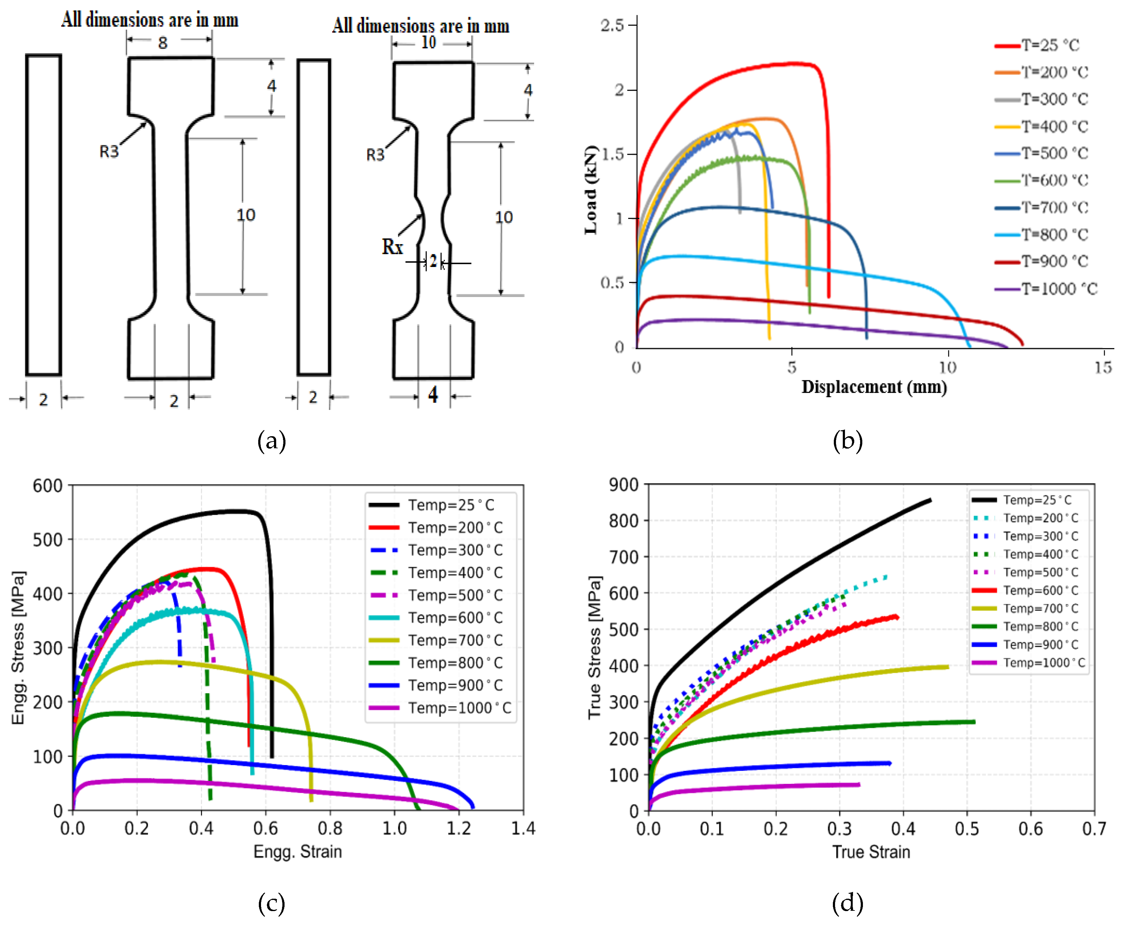
Figure 2.
(a) Load-displacement data as obtained from tests of notched tensile specimens of different notch radii and their comparison with data of smooth tensile specimen; (b) Effect of notch radius on maximum load carrying capacity of notched tensile specimens and average fracture strain; (c) Variation of yield strengh and (d) Ultimate tensle strength of SS316LN with test temperature as obtained from tensile tests and its comparison with French nuclear reactor design code RCC-MR data.
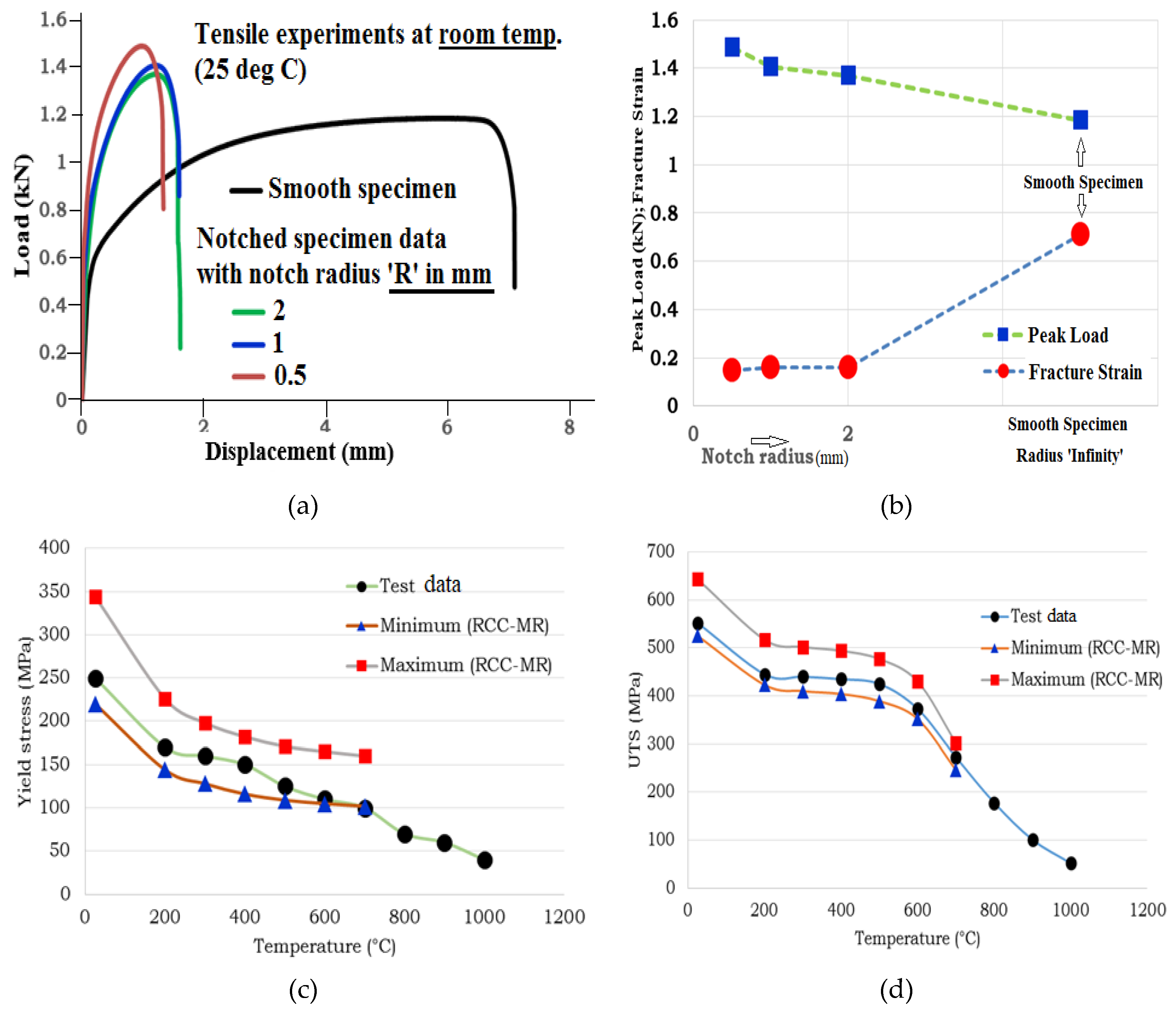
Figure 3.
(a) Schematic presentation of Johnson-Cook plasticity model and damage model through stress-strain response of a material; (b) Effect of strain rate and temperature on material stress-strain curve.
Figure 3.
(a) Schematic presentation of Johnson-Cook plasticity model and damage model through stress-strain response of a material; (b) Effect of strain rate and temperature on material stress-strain curve.
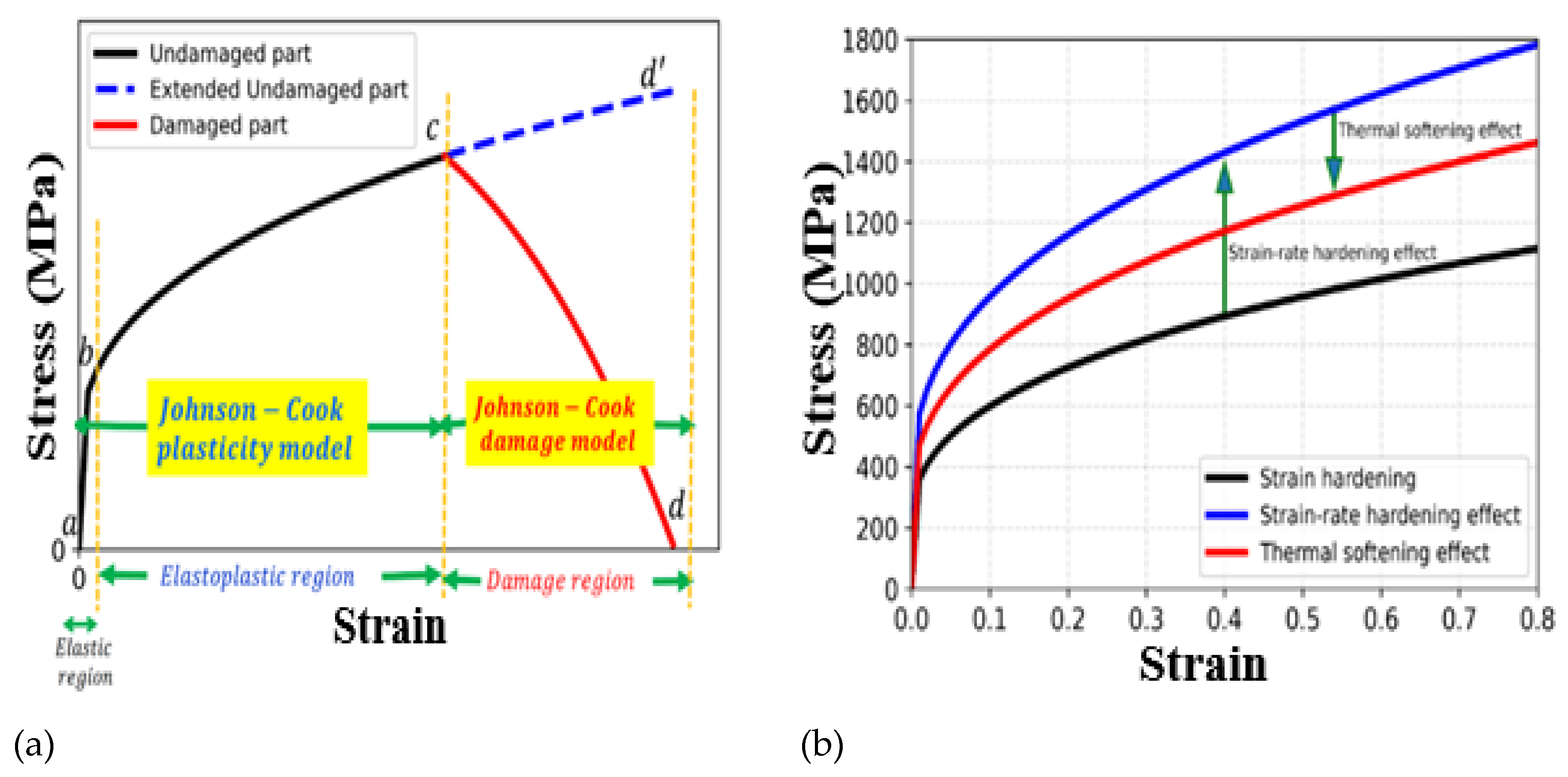
Figure 4.
Effect of three different plasticity parameters of Johnson-Cook model on stress-strain response of a material. (a) Effect of parameter ‘A’; (b) Effect of parameter ‘B’; and (c) Effect of parameter ‘n’ on stress-strain response.
Figure 4.
Effect of three different plasticity parameters of Johnson-Cook model on stress-strain response of a material. (a) Effect of parameter ‘A’; (b) Effect of parameter ‘B’; and (c) Effect of parameter ‘n’ on stress-strain response.
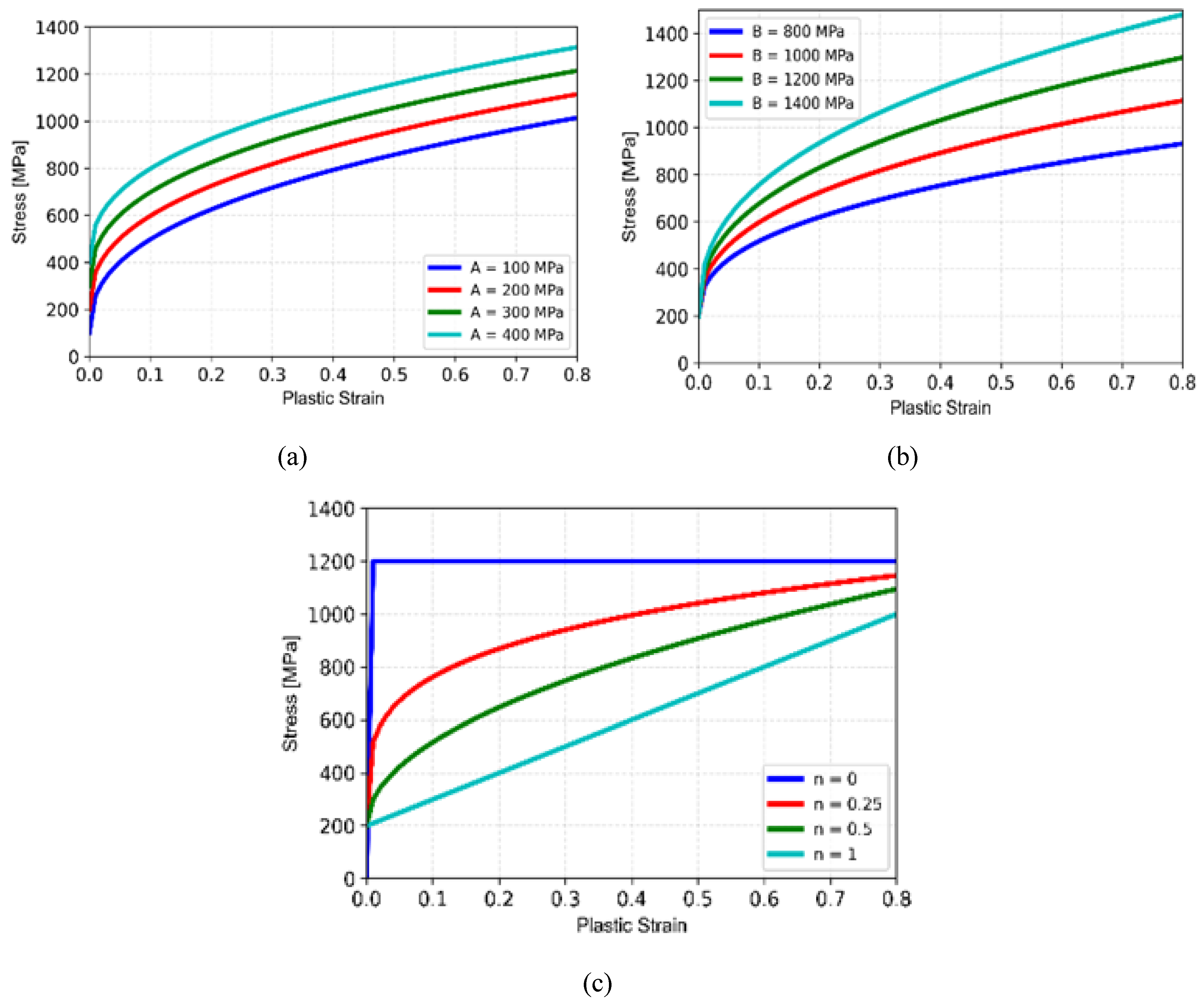
Figure 5.
(a) 3D finite element mesh of smooth tensile specimens as used in experiments; (b-d) Effect of Johnson-Cook model parameters A, B and ‘n’ on load-displacement response of smooth tensile specimen.
Figure 5.
(a) 3D finite element mesh of smooth tensile specimens as used in experiments; (b-d) Effect of Johnson-Cook model parameters A, B and ‘n’ on load-displacement response of smooth tensile specimen.
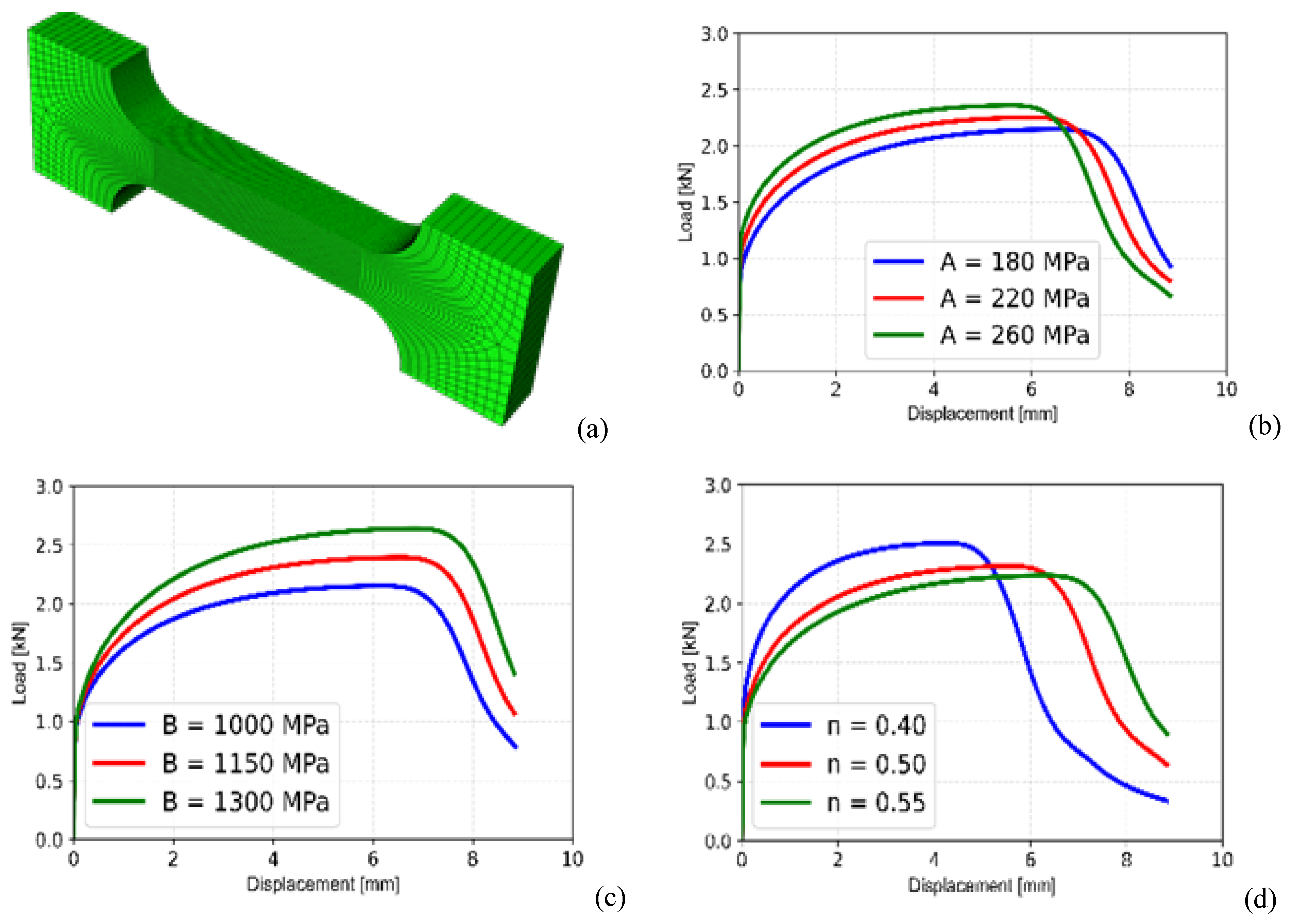
Figure 6.
(a) 3D finite element mesh of the notched tensile specimen with 1 mm notch radius as used in experiments; (b-d) Effect of Johnson-Cook model parameters A, B and ‘n’ on load-displacement response of the notched tensile specimen.
Figure 6.
(a) 3D finite element mesh of the notched tensile specimen with 1 mm notch radius as used in experiments; (b-d) Effect of Johnson-Cook model parameters A, B and ‘n’ on load-displacement response of the notched tensile specimen.
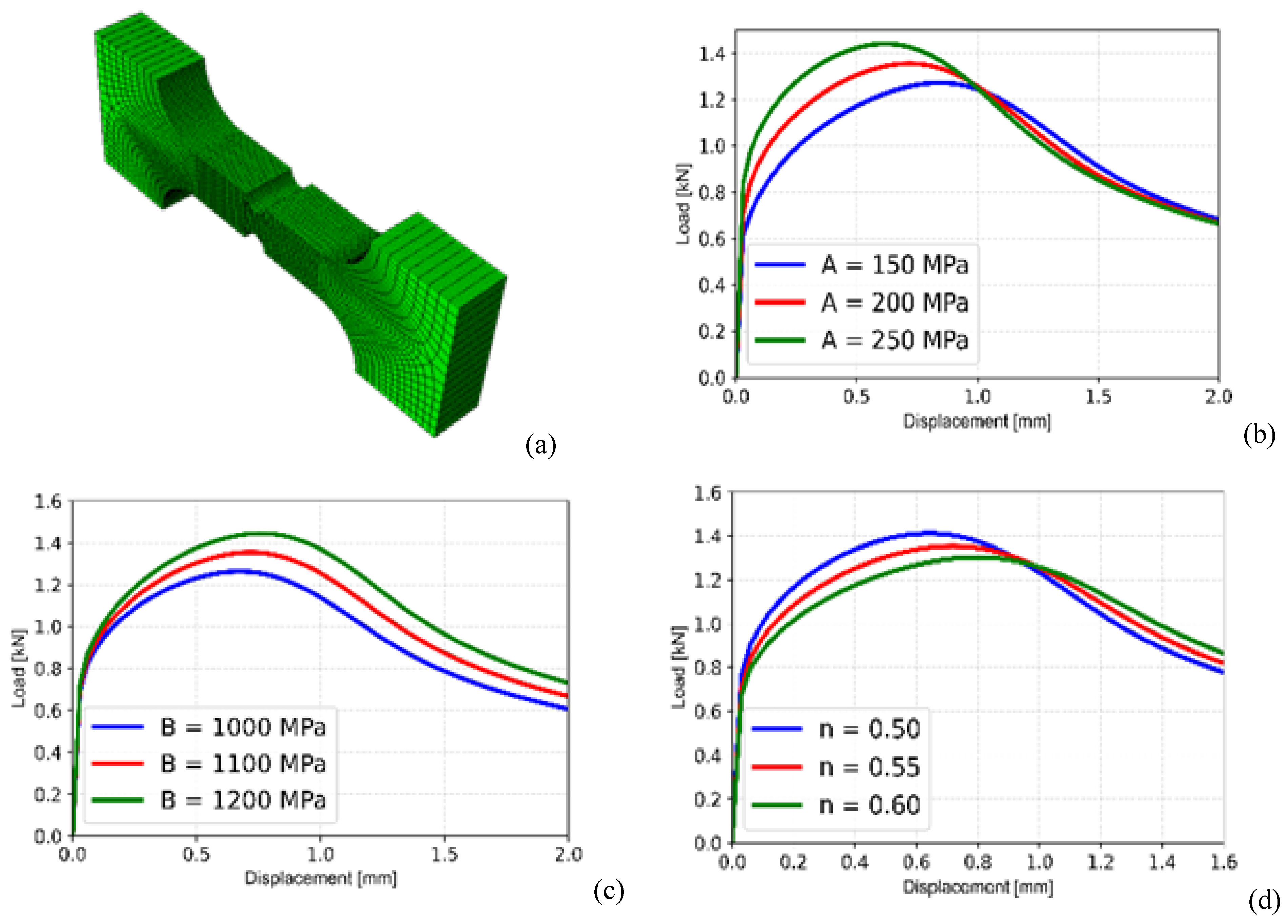
Figure 7.
(a) Schematic arrangement of specimen, striker and the bars in Split-Hopkinson Pressure Bar (SHPB) test setup; Effect of (b) mesh size of the specimen and (c) Johnson-Cook model strain-rate-dependent paremeter ‘C’ on incident, transmitted and reflected microstrain vs time signal as obtained from FE analysis of SHPB test; (d) Evaluation of Johnson-Cook plasticity parameters A, B and ‘n’ from quasistatic stress-strain data; (e) Comparison of load-displacement data of SHPB test with that predicted using FE analysis.
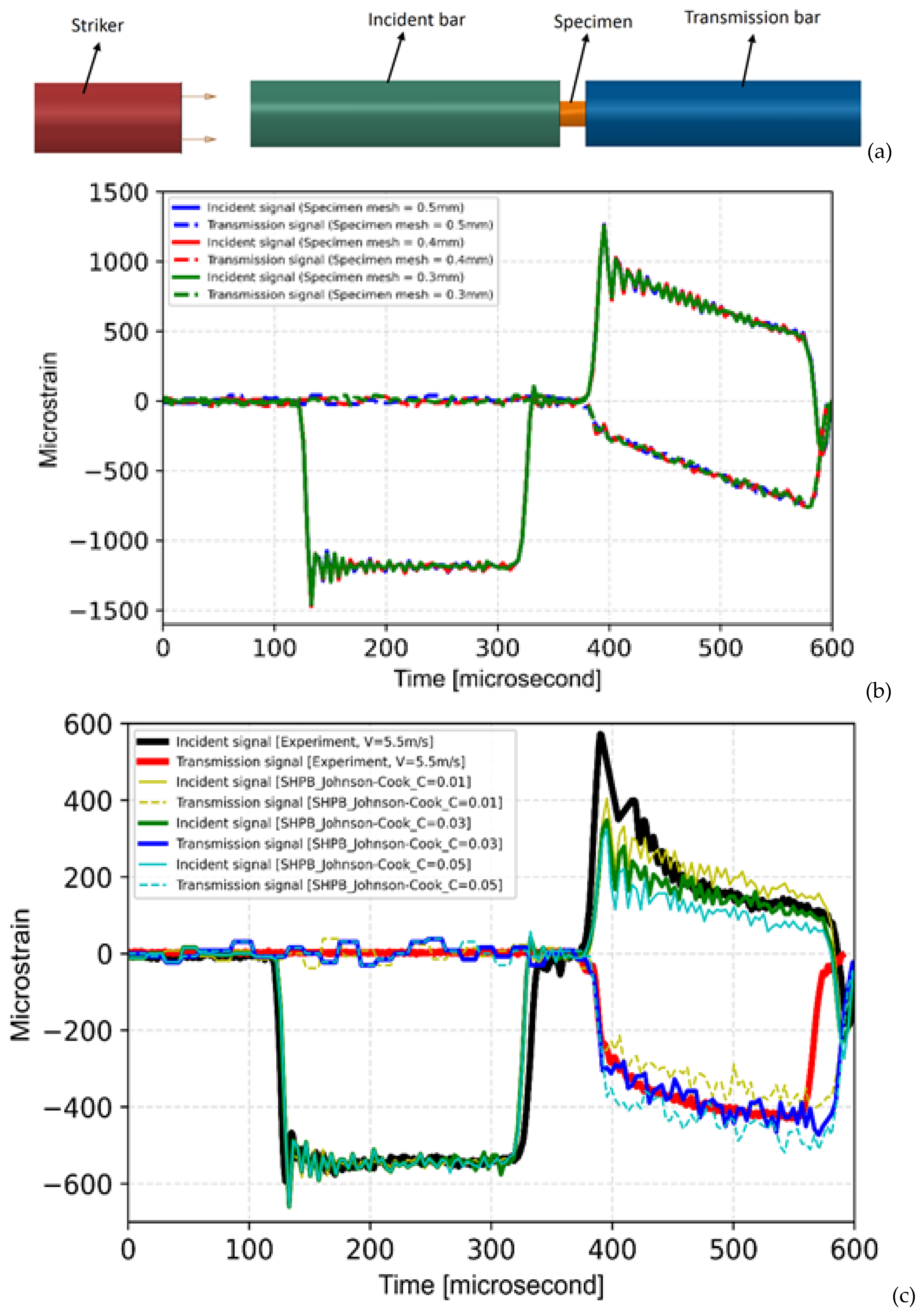
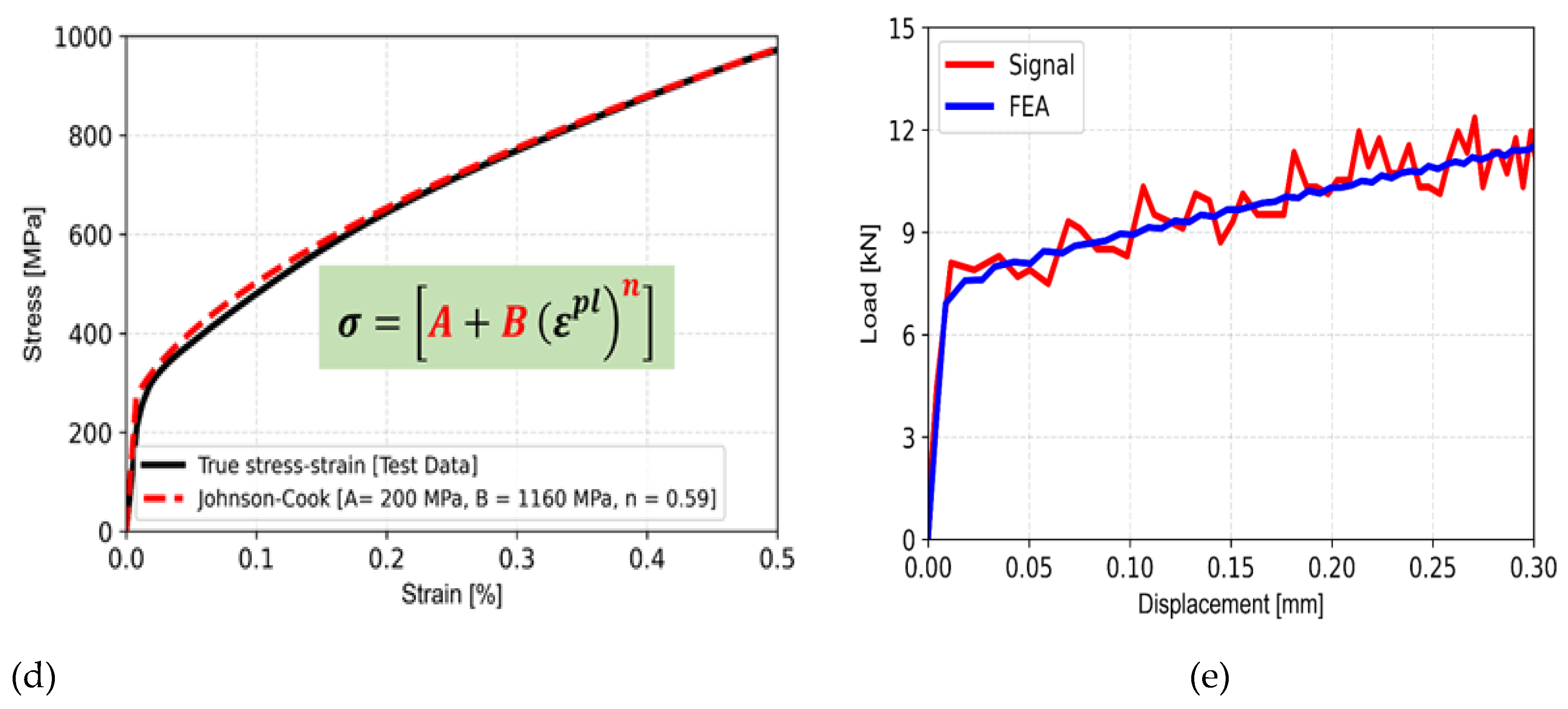
Figure 8.
(a) Evaluation of Johnson-Cook temperature-dependent parameter ‘m’ using tensile test data at different temperatures; Comparison of load-displacement response of the smooth tensile test as obtained from FE analysis using Johnson-Cook model with experimental data for test temperatures of (b-d) 300oC, 400oC and 600oC respectively.
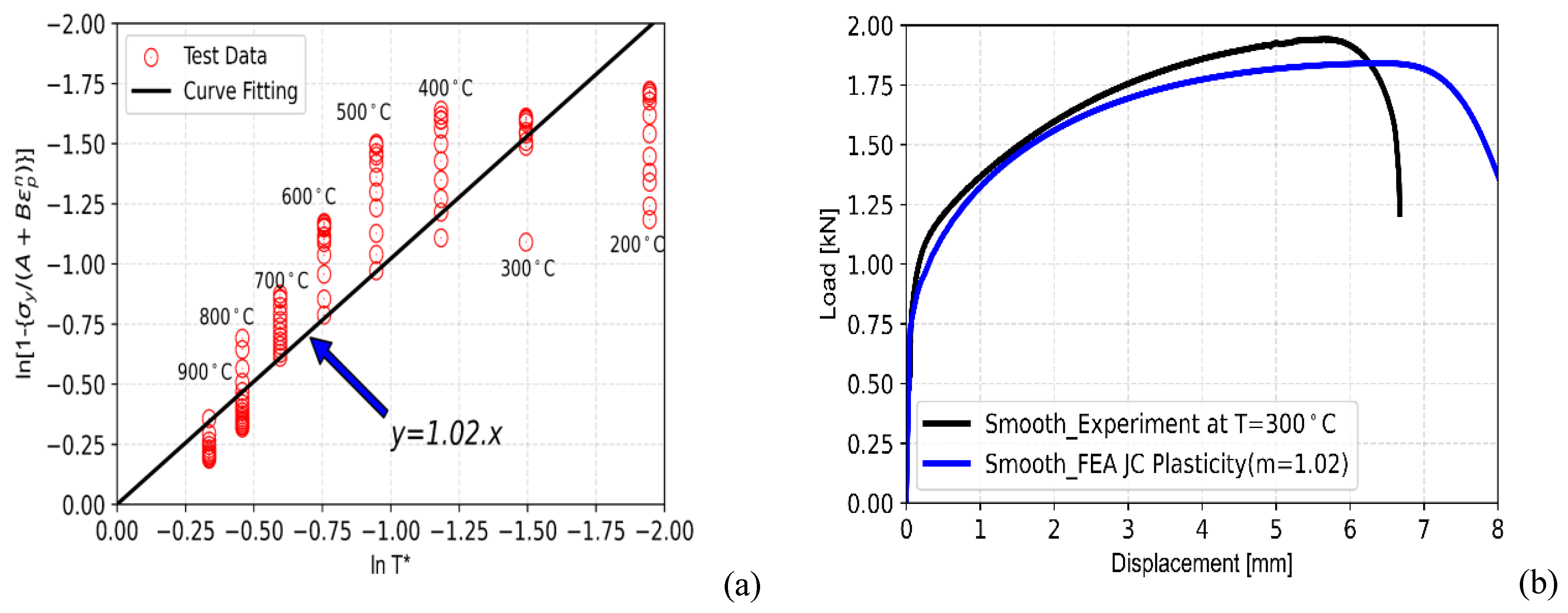
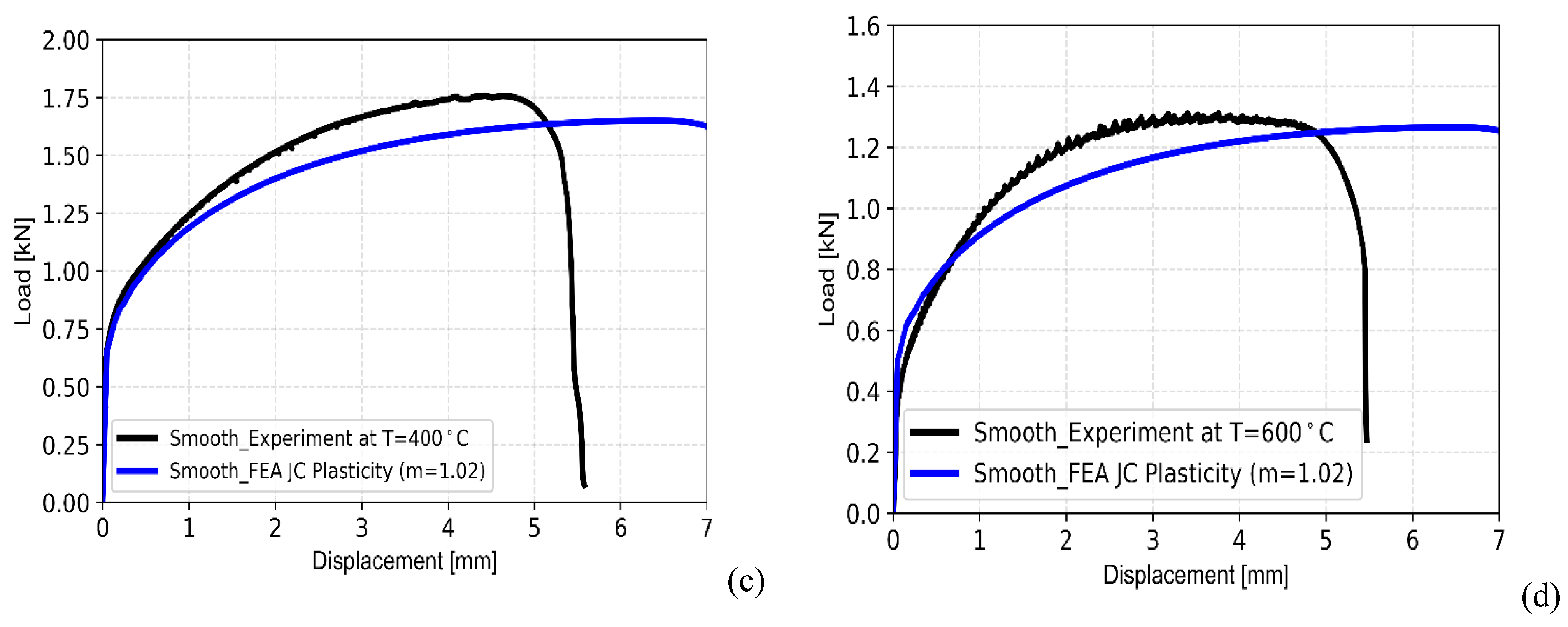
Figure 9.
(a) Effect of variation of Johnson-Cook temperature-dependent parameter ‘m’ on load-displacement curve of smooth tensile specimen; (b) Variation of error in the load-displacement data as obtained from FE analysis of smooth tensile specimen (w.r.t. experimental data) with change in parameter ‘m’; Comparison of load-displacement data of smooth tensile specimen as obtained from FE analysis (using two different values of Johnson-Cook temperature-dependent parameter ‘m’) with experimental data for test temperatures of (c-d) 300oC, 400oC and 600oC respectively.
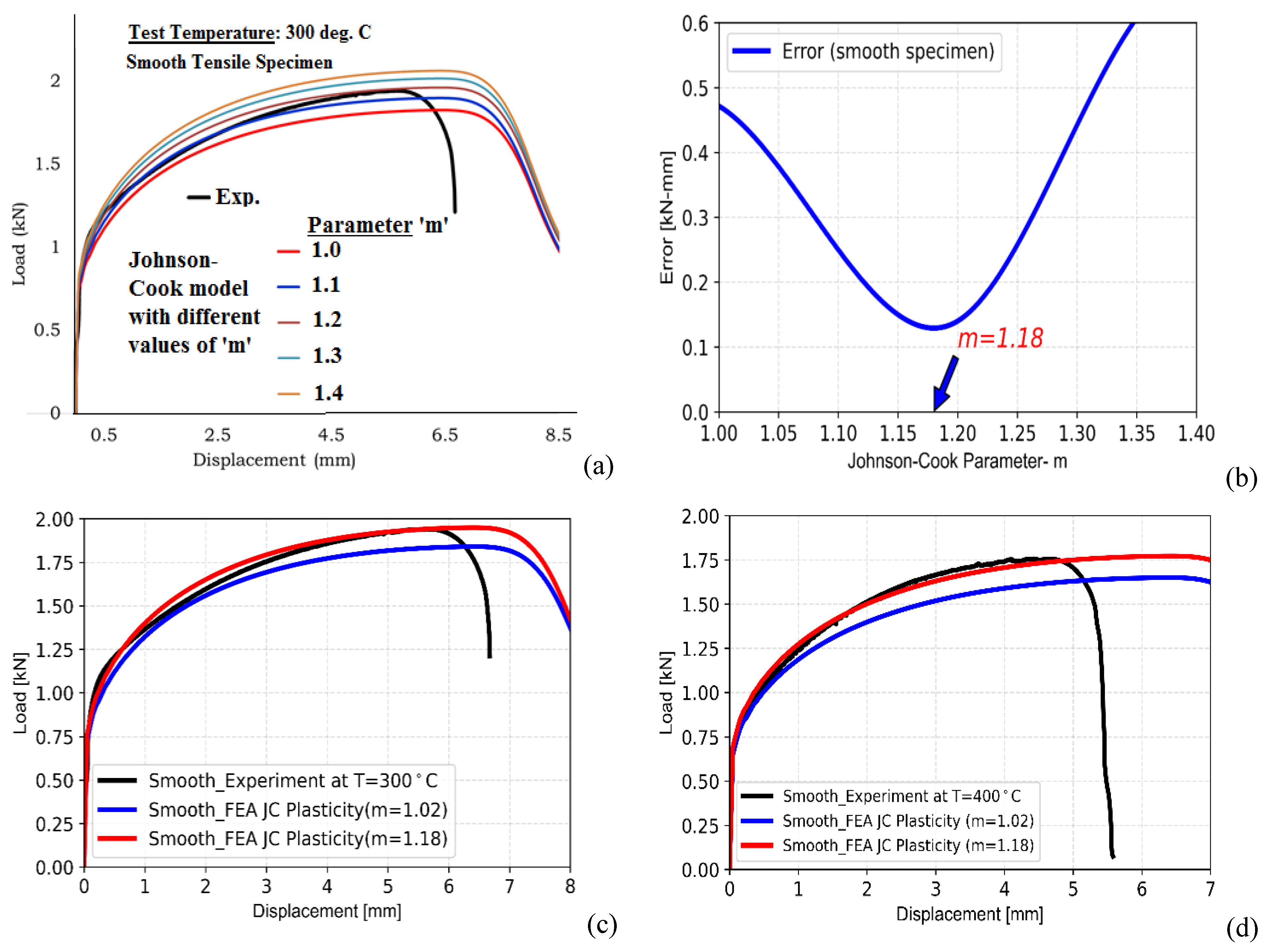
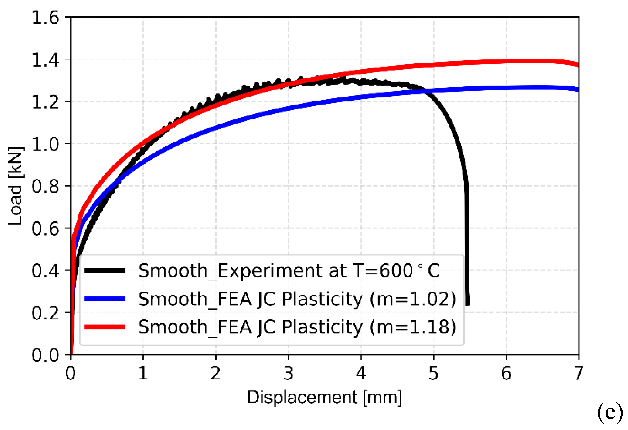
Figure 10.
Effect of (a) yield strength and (b) parameter ‘n’ and ‘α’ on material stress-strain curve modelled with Ramberg-Osgood material model.
Figure 10.
Effect of (a) yield strength and (b) parameter ‘n’ and ‘α’ on material stress-strain curve modelled with Ramberg-Osgood material model.
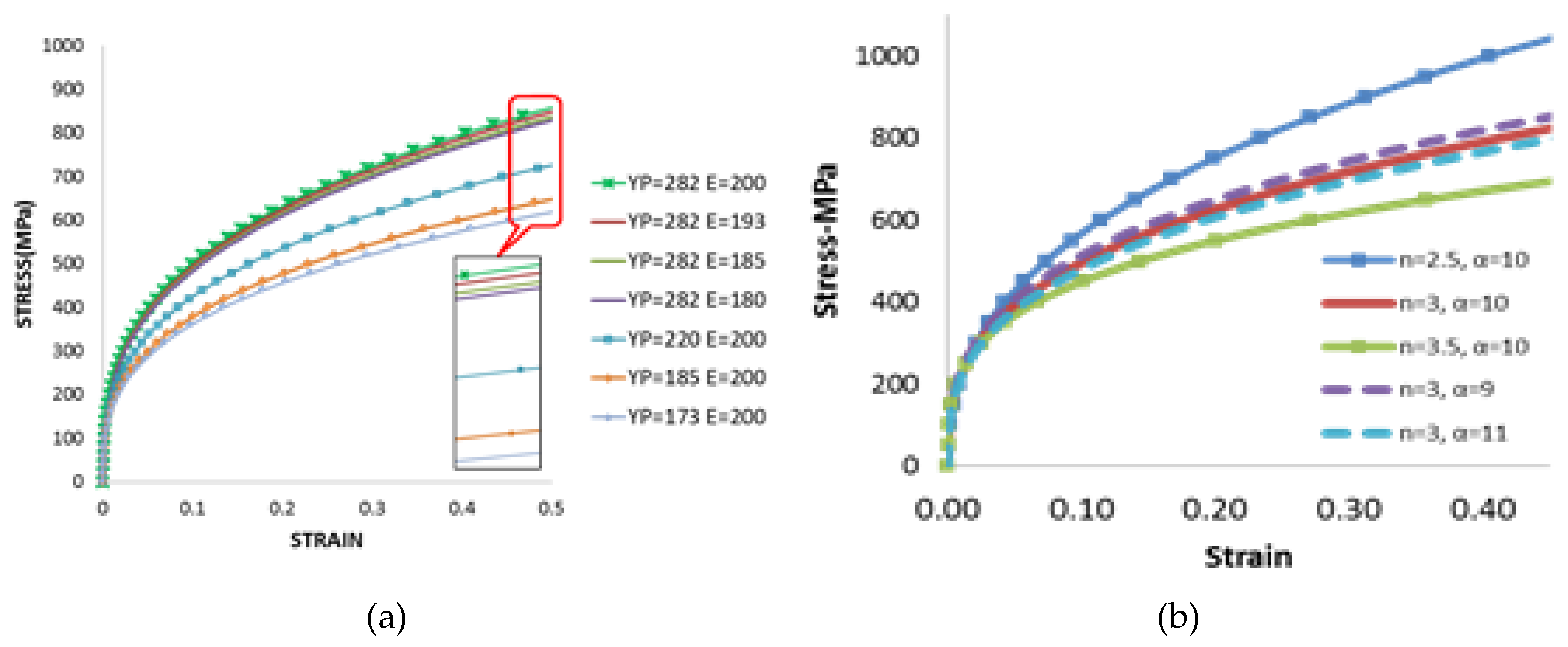
Figure 11.
(a) Load-displacement data as obtained from testing of smooth and notched tensile specimens of SS316LN at room temperature; (b) A typical comparison of load-displacement data as obtained from from analysis of notched tensile specimen with that of experiment and evaluation of error between FE analysis and experiment; (c) Variation of normalized error with Ramberg-Osgood parameter ‘n’ for a given value of parameter ‘α’, (d) Different combinations of Ramberg-Osgood parameter ‘n’ and ‘α’ corresponding to minimum values of normalized error as obtained from error analysis between FEM and experiment; Variation of normalized error with Ramberg-Osgood parameter ‘n’ and the corresponding values of ‘α’ as depicted in (d) for analysis at (e) room temperature (25oC) and (f) 650oC.
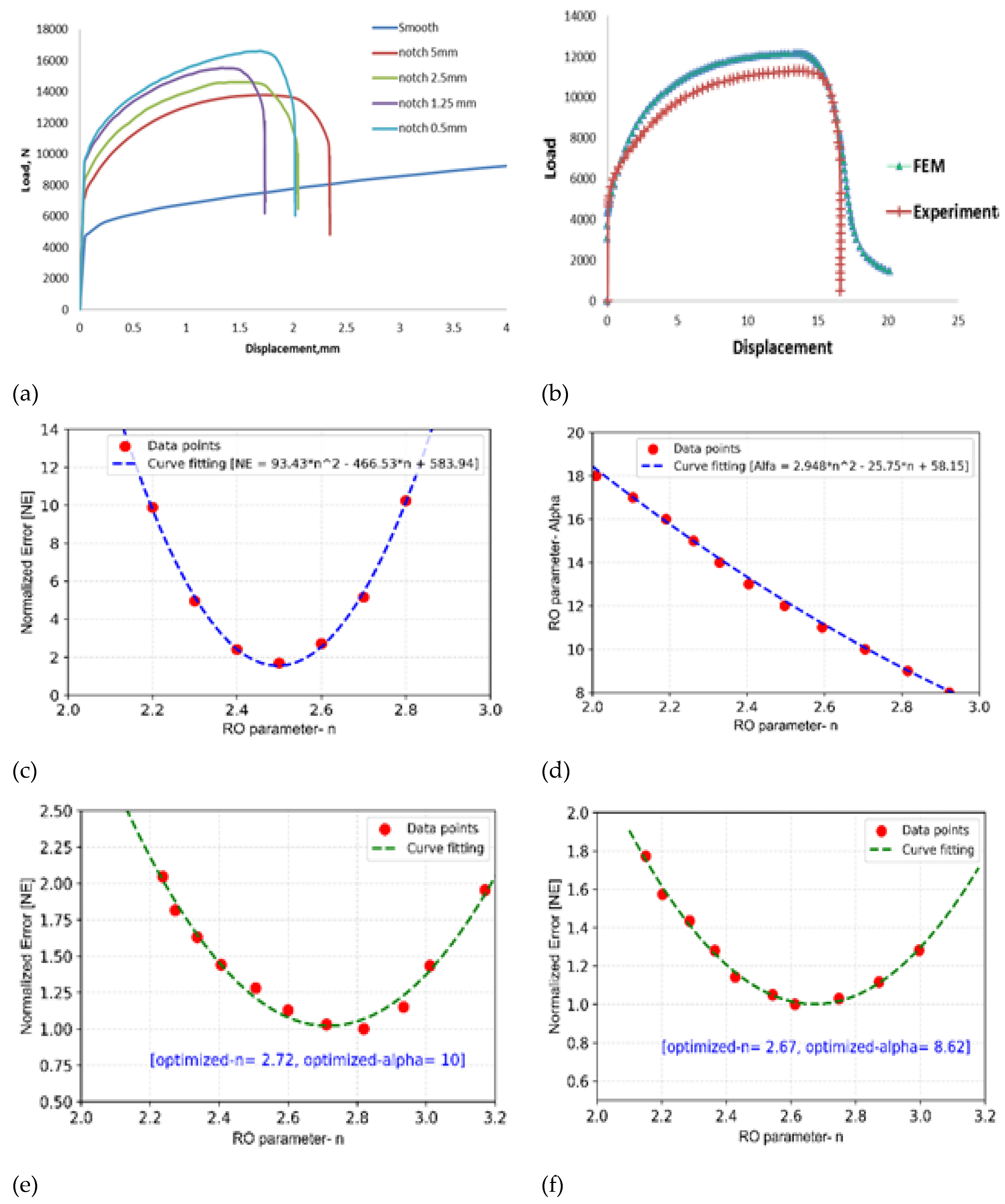
Figure 12.
Variation of Ramberg-Osgood paramters (a) ‘n’ and (b) ‘α’ with yield strength of material SS316LN as obtained from the optimization algorithm developed in this work and comparison of data with those of RCC-MR code.
Figure 12.
Variation of Ramberg-Osgood paramters (a) ‘n’ and (b) ‘α’ with yield strength of material SS316LN as obtained from the optimization algorithm developed in this work and comparison of data with those of RCC-MR code.
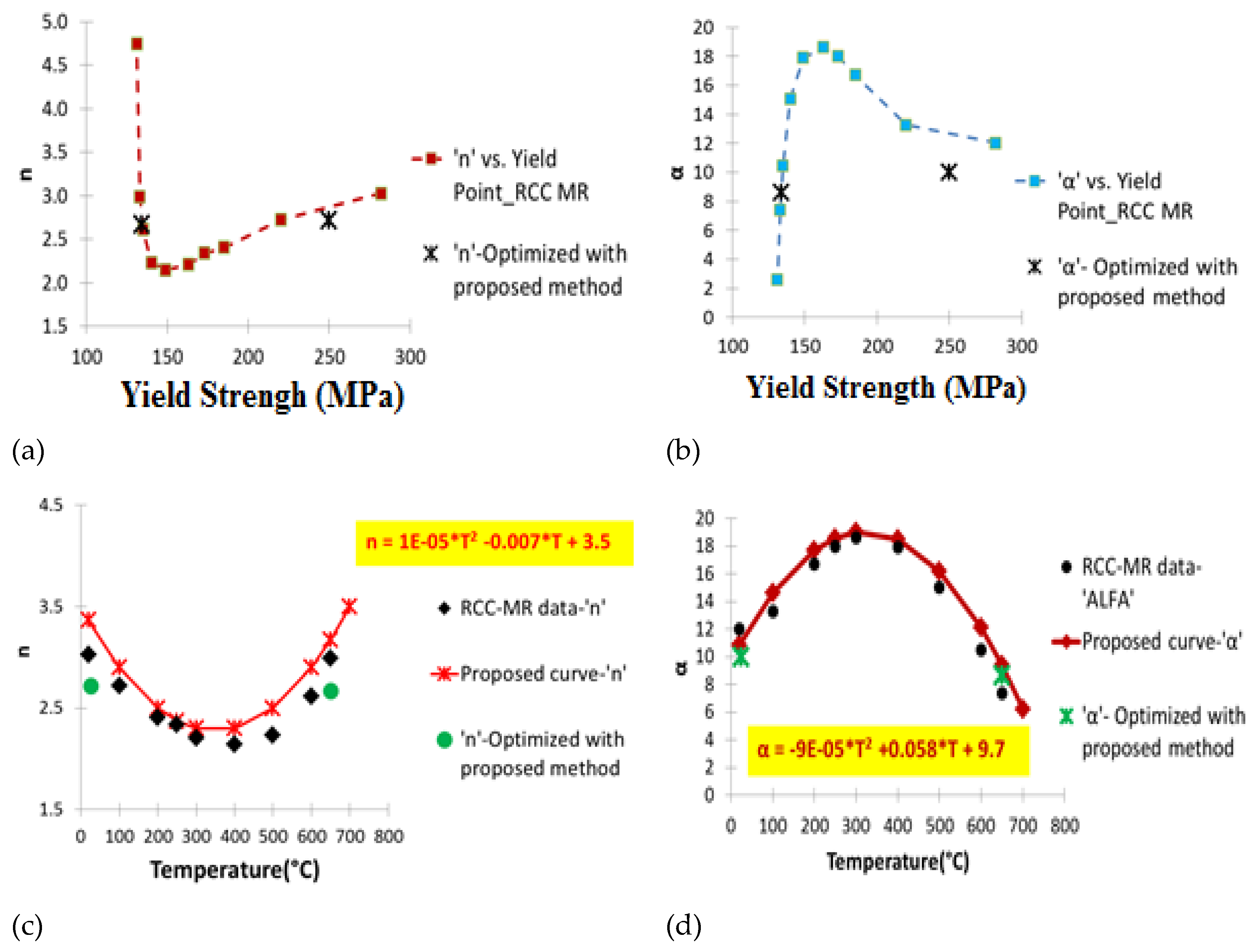
Figure 13.
Comparison of load-displacement data as obatained from FE analysis of (a-b) Smooth tensile specimen, and notched tensile specimens with (c-d) 5 mm notch radius; (e-f) 2.5 mm notch radius; (g-h) 1.25 mm notch radius; (i-j) 0.5 mm notch radius with Ramberg-Osgood material parameter (evaluated using two different methods) with that of experiment at two different temperatures (25oC and 650oC).
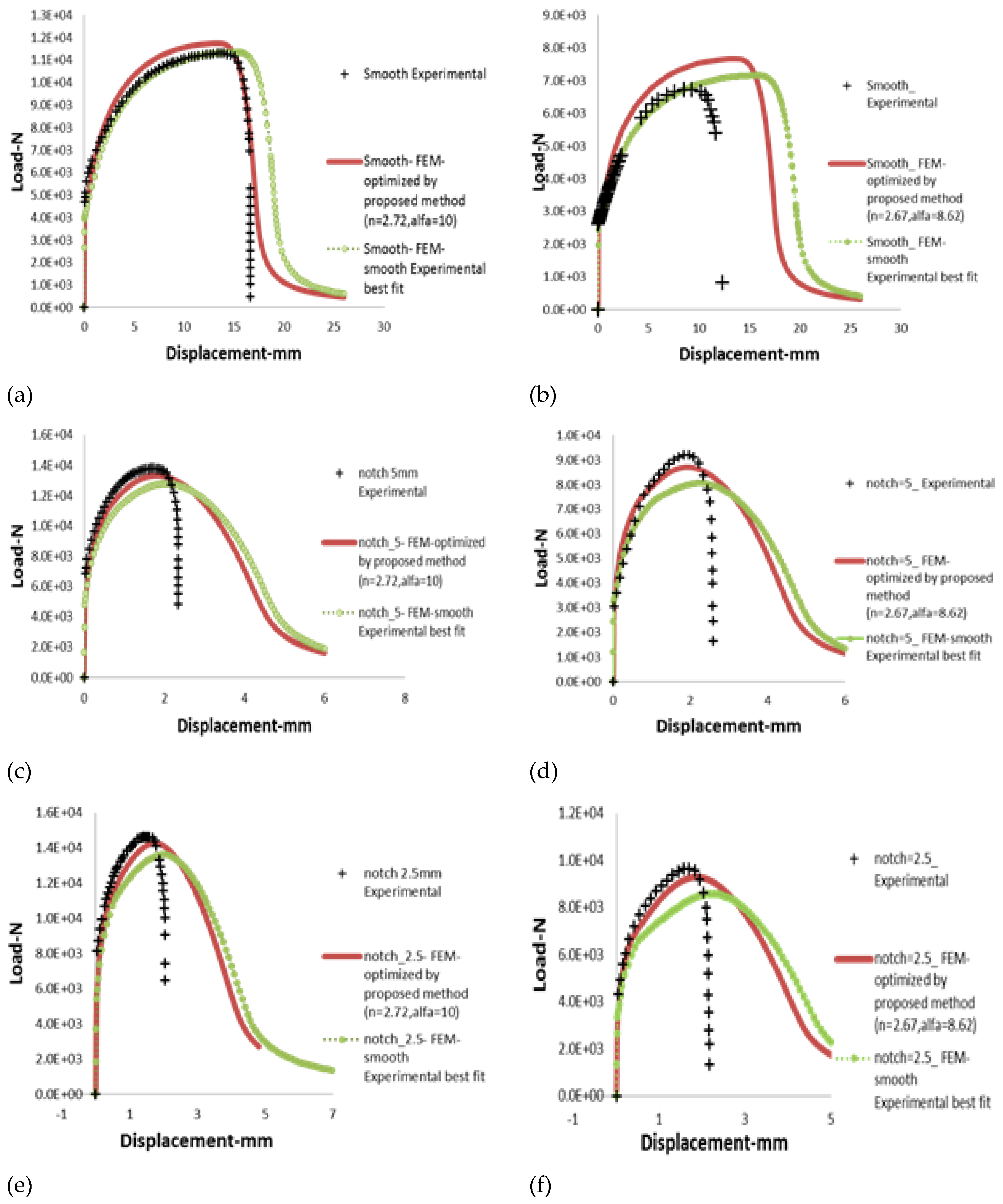
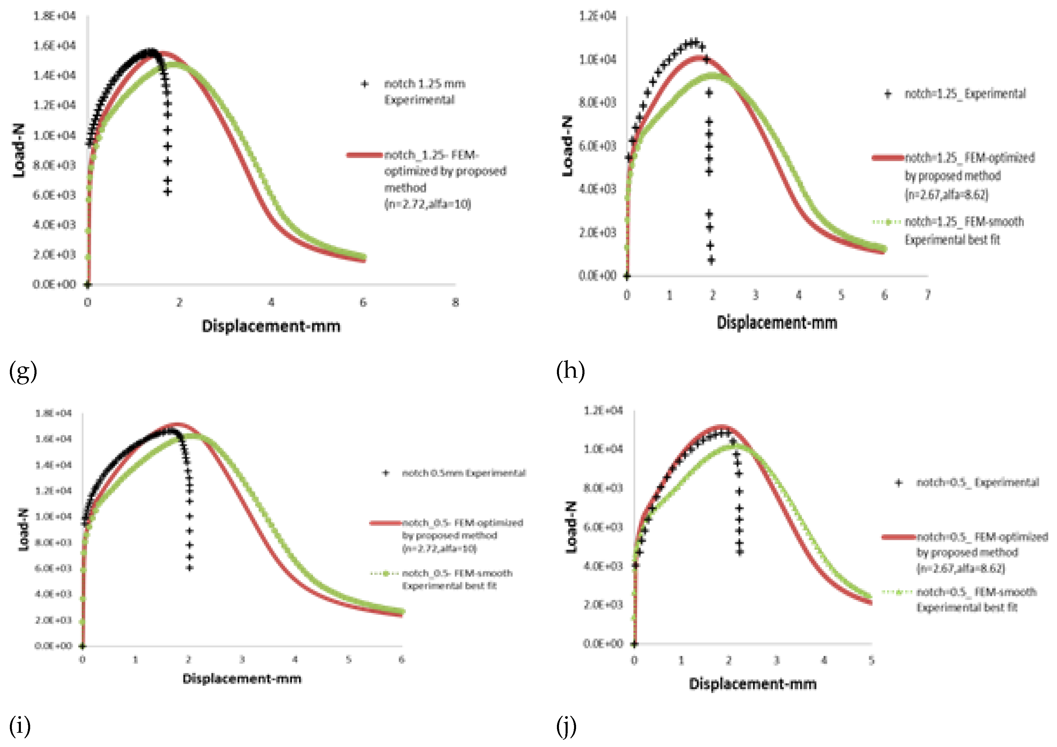
Figure 14.
(a) Typical contour of stress triaxiality in (a) flat tensile specimen and (b) notched tensile specimen with 1 mm notch radius; (c) Variation of stress triaxiality at the central cross-section of notched tensile specimens with notch radii of 2, 1 and 0.5 mm plotted along width or notch and thickness directions respectively; Contour variation of equivalent plastic strain in (d) smooth tensile and (e) notched tensile specimen (with 1 mm notch radius) for a given loading.
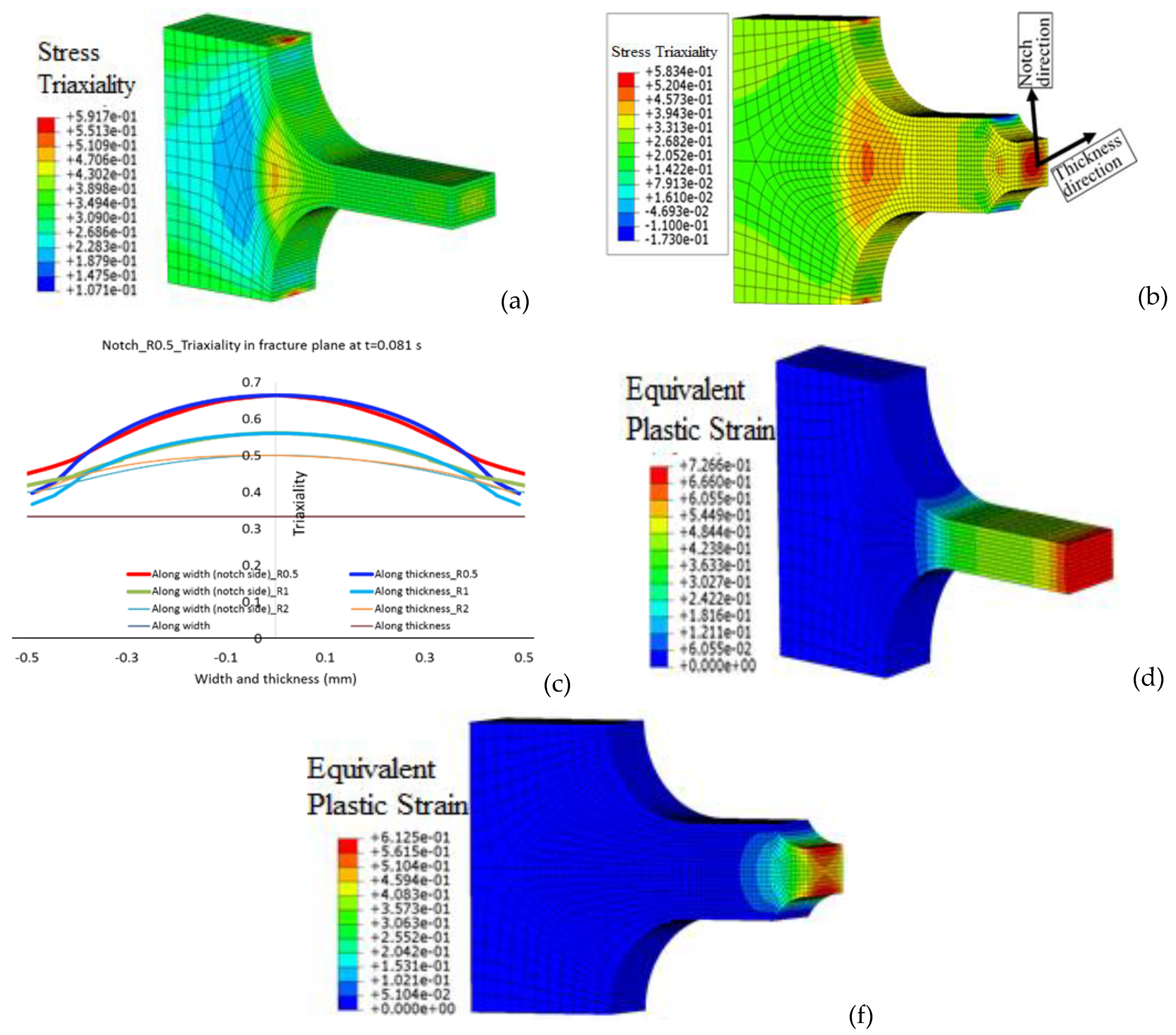
Figure 15.
Variation of (a) load carrying capacities of smooth and notched tensile specimens as a function of applied displacement (varying linearly with pseudo-time); Variation of (b) stress triaxiality and (c) equivalent plastic strain at the centres of smooth and notched tensile spcimens with applied loading.
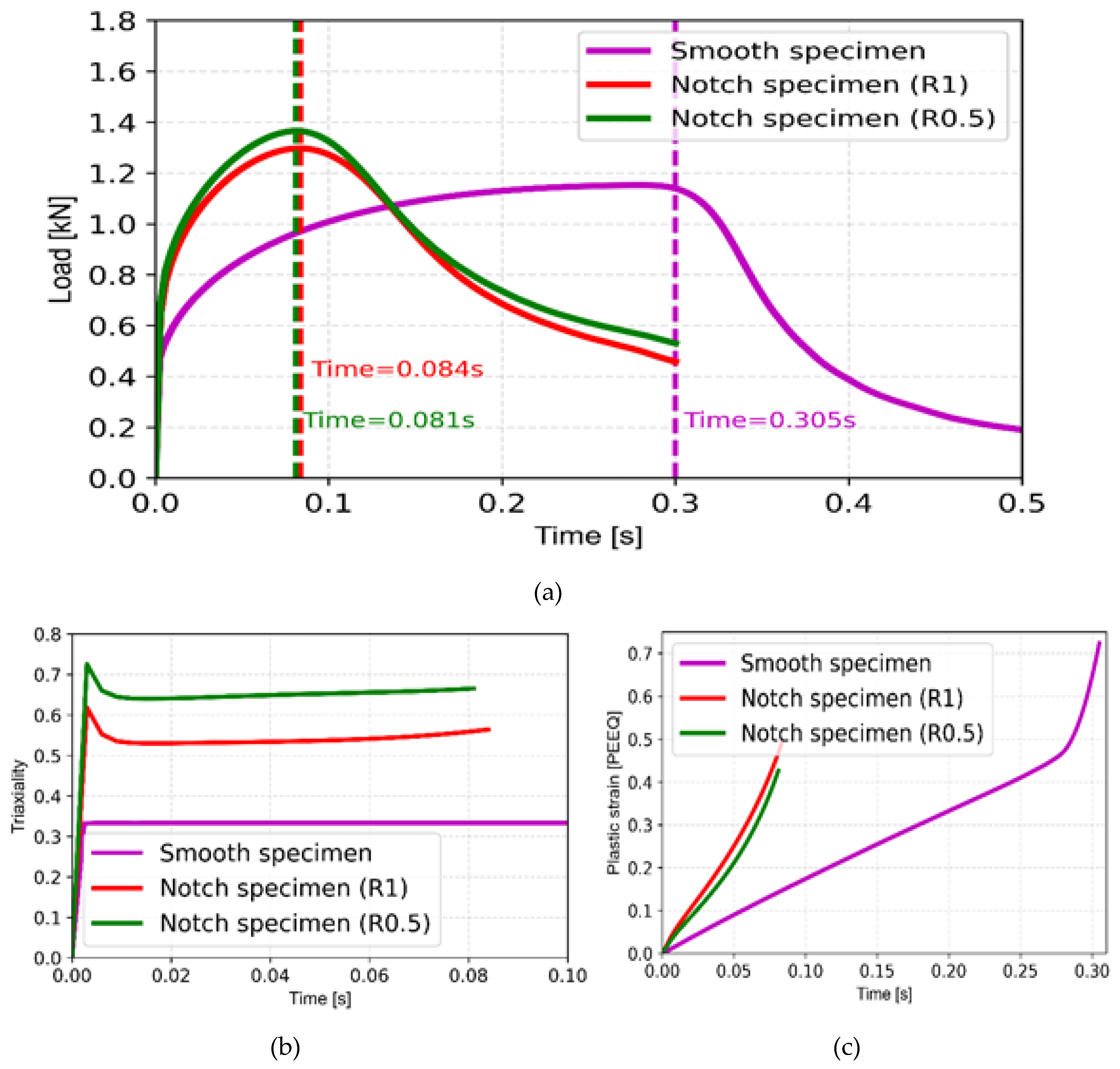
Figure 16.
(a) Variation of fracture strain as a function of stress triaxiality as obtained from combined FE analysis and experimental data and use of the same to evaluate Johnson-Cook damage model parameters d1, d2 and d3; (b) Use of experimental data at different temperatures to evaluate Johnson-Cook damage model parameter d5.
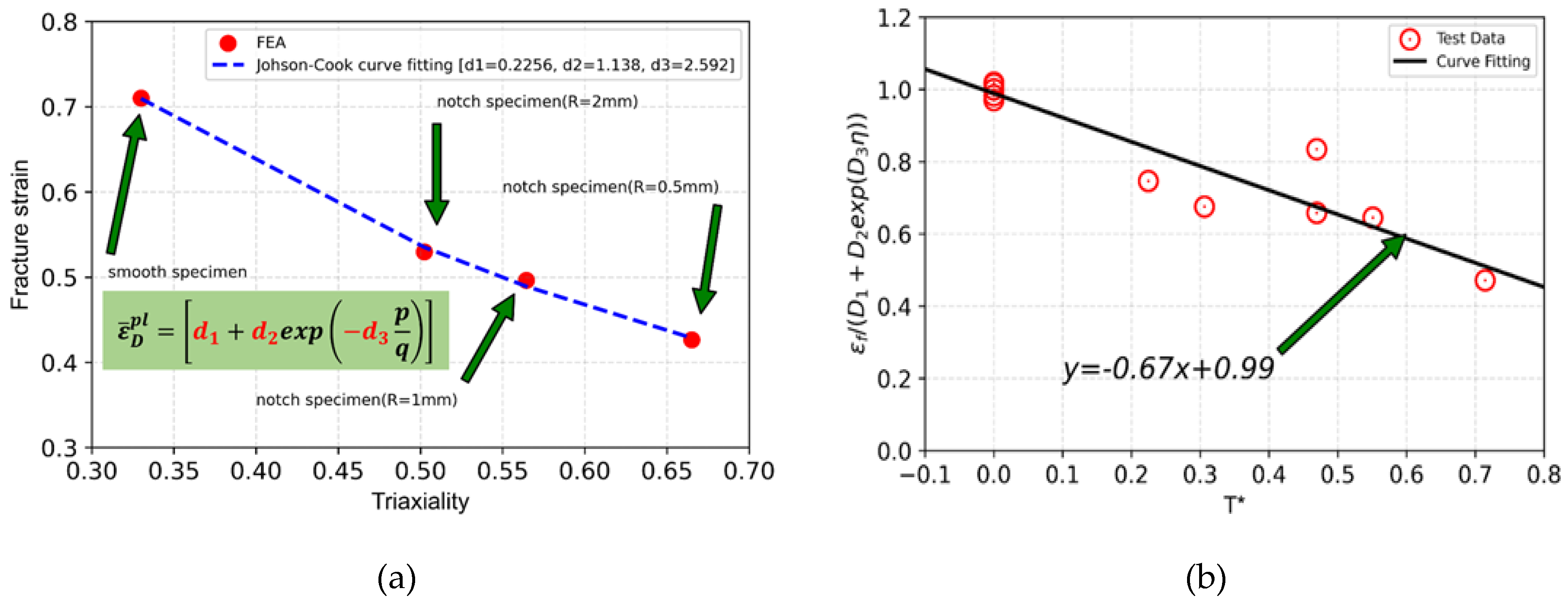
Figure 17.
Effect of Johnson-Cook damage model parameters d5 on load-displacement response of smooth tensile specimen as obtained from FE analysis at a typical temperature of 300oC and its comparison with experimental data; (b) Variation of error (i.e., absolute difference between experimental and FE analysis load-displacement data) as a function of parameter d5; (c-h) Comparison of load-displacement response of different types of specimens at different test temperatures (c-smooth tensile at 25oC; d-notched tensile specimen with 1 mm notch radius at 25oC; e- notched tensile specimen with 0.5 mm notch radius at 25oC; f- smooth tensile at 300oC; g- smooth tensile at 400oC; h- smooth tensile at 600oC) as obtained from FE analysis (using two different values of Johnson-Cook damage model parameters d5) with that of experiment.
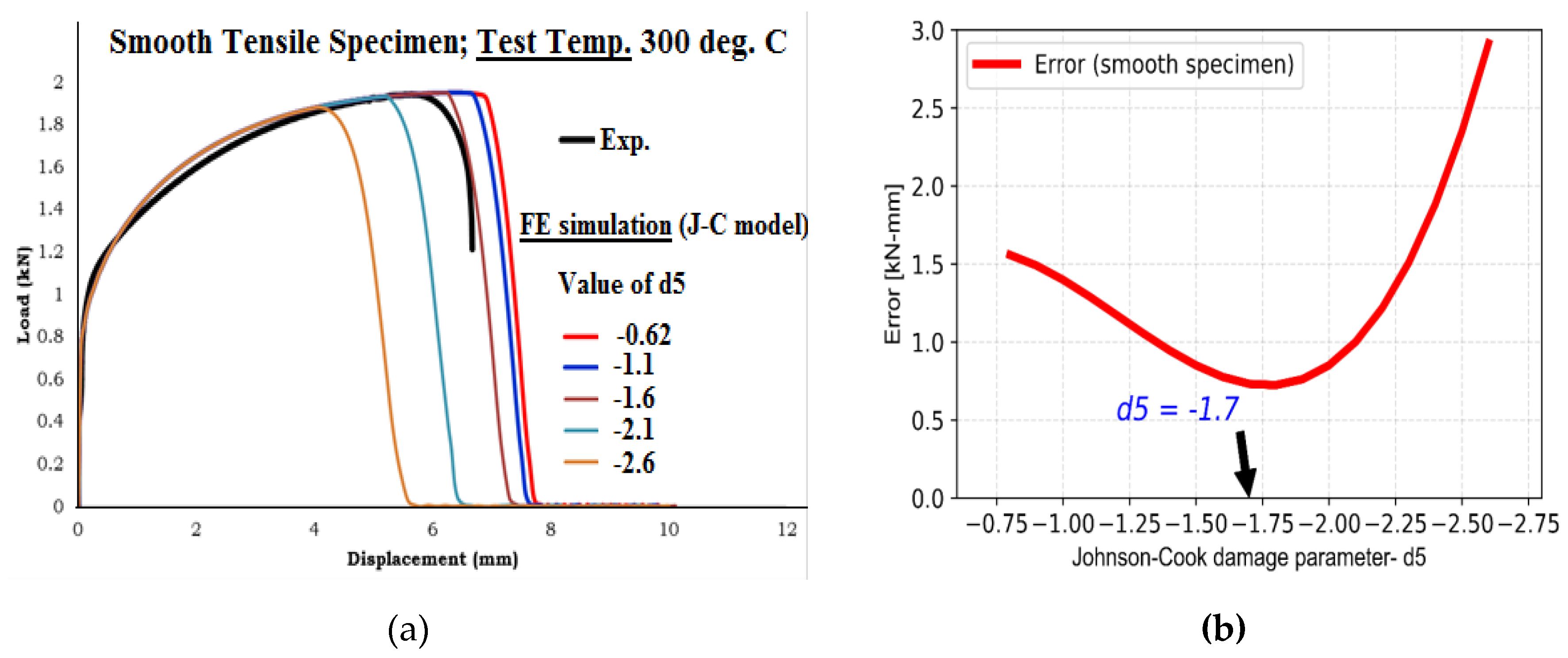
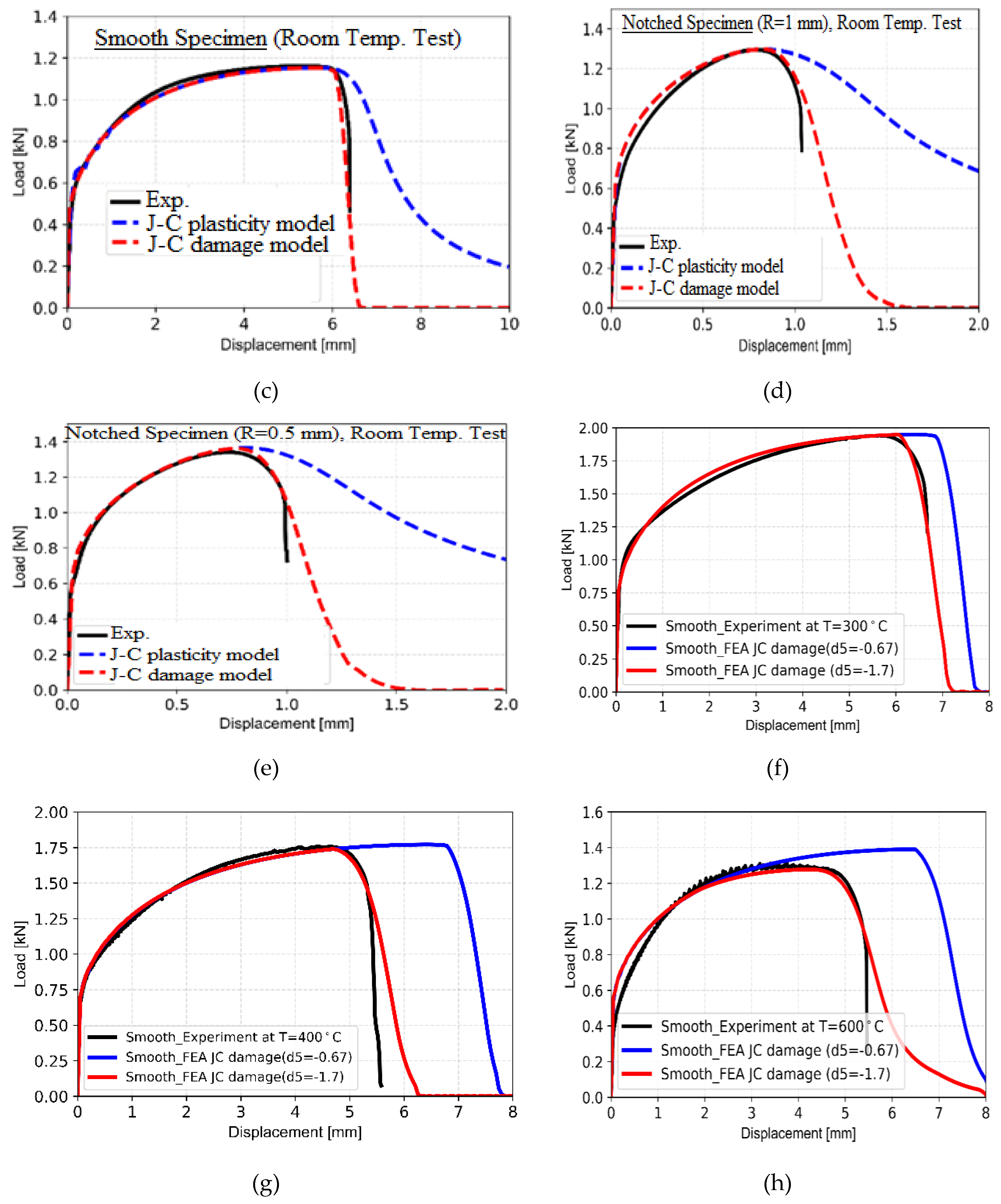

Table 1.
Chemical composition of austenitic stainless steel SS316LN used in Indian PFBR.
| Element | C | Cr | Ni | Mo | N | Mn | Si | P | S | Ti | Nb | Cu | Co | B |
|---|---|---|---|---|---|---|---|---|---|---|---|---|---|---|
| Wt. % | 0.02-0.03 | 17-18 | 12-12.5 | 2.3-2.7 | 0.06-0.08 | 1.6-2.0 | 0.5 | 0.03 | 0.01 | 0.05 | 0.05 | 1.0 | 0.25 | 0.002 |
Table 2.
Variation of absolute difference in area of load-displacement curves of experiment and FE analysis for various values of parameter ‘m’.
Table 2.
Variation of absolute difference in area of load-displacement curves of experiment and FE analysis for various values of parameter ‘m’.
| Johnson-Cook Parameter ‘m’ | Area_Test (kN-mm) | Area_FEA (kN-mm) | Error = Absolute Difference (kN-mm) |
| 1 | 9.27 | 8.8 | 0.47 |
| 1.1 | “ | 9.15 | 0.12 |
| 1.2 | “ | 9.45 | 0.18 |
| 1.3 | “ | 9.71 | 0.44 |
| 1.4 | “ | 9.94 | 0.67 |
Table 3.
Variation of absolute difference in area of load-displacement curves of experiment and FE analysis for various values of parameter d5.
Table 3.
Variation of absolute difference in area of load-displacement curves of experiment and FE analysis for various values of parameter d5.
| Value of Parameter D5 | Area_Experiment (kN-mm) | Area_FEA (kN-mm) | Error = Absolute Difference (kN-mm) |
|---|---|---|---|
| -0.6 | 11.14 | 12.71 | 1.58 |
| -1.1 | “ | 12.48 | 1.35 |
| -1.6 | “ | 11.82 | 0.69 |
| -2.1 | “ | 10.07 | 1.06 |
| -2.6 | “ | 8.23 | 2.91 |
Table 4.
Johnson-Cook plasticity and damage parameters for austenitic strainless steel SS316LN used in Indian PFBR.
Table 4.
Johnson-Cook plasticity and damage parameters for austenitic strainless steel SS316LN used in Indian PFBR.
| Johnson-Cook Plasticity PARAMETERS | |
|---|---|
| Parameter | Value |
| A | 200 MPa |
| B | 1160 MPa |
| n | 0.59 |
| C (ref. strain rate=1.0e-3) | 0.03 |
| m (Tref=25oC) | 1.18 |
| Johnson-Cook damage Parameters | |
| d1 | 0.225 |
| d2 | 1.138 |
| d3 | 2.592 |
| d5 (Tref=25oC) | -1.7 |
Disclaimer/Publisher’s Note: The statements, opinions and data contained in all publications are solely those of the individual author(s) and contributor(s) and not of MDPI and/or the editor(s). MDPI and/or the editor(s) disclaim responsibility for any injury to people or property resulting from any ideas, methods, instructions or products referred to in the content. |
© 2024 by the authors. Licensee MDPI, Basel, Switzerland. This article is an open access article distributed under the terms and conditions of the Creative Commons Attribution (CC BY) license (http://creativecommons.org/licenses/by/4.0/).
Copyright: This open access article is published under a Creative Commons CC BY 4.0 license, which permit the free download, distribution, and reuse, provided that the author and preprint are cited in any reuse.


