
Submitted:
26 December 2024
Posted:
27 December 2024
You are already at the latest version
Abstract
Previously we extended the definition of spin 12 by including coherence in addition to the usual polarization. This followed after noting that the geometric product of two Pauli spin components has contributions from both a Pauli vector and a Pauli bivector, but the Dirac equation has no bivector. Introducing one complexifies the Dirac field, leading to the definition of helicity which is the complementary property to spin polarization. The resulting symmetry change leads to the resolution of the EPR paradox and disproves Bell’s Theorem. In this paper, we expand on the symmetry and parity arguments which support quaternion, or Q-spin. We relate it to Twistor theory, and discuss the implication on Dirac’s matter-antimatter production. We show that Q-spin has a number of similarities with a photon. We summarize the symmetry breaking where the classical domain bifurcates into complementary quantum domains of matter and torques.
Keywords:
quaternion spiin
; dirac field
; EPR paradox
; quantum coherence
; wave-particle duality
; antimatter
; Baryogenesis
; Bell’s Theory
; quantum computing
; anyons
; Twistor
; quantum theory
MSC: 81P40
1. Introduction
Recently we introduced quaternion spin, [1], which is a consequence of complexifying the Dirac field and introducing its structure as a bivector. This changes spin symmetry from SU(2) to the quaternion group, . Rather than two spins with two polarized states each: a matter-antimatter pair, the complex field introduces spin helicity as the complementary property to spin polarization. It can then describes one particle with four states: two polarized states and two helicity states. Dirac’s two point particles becomes a single two dimensional spin with a bivector structure. We call this quaternion, or Q-spin. The purpose of this paper is to discuss its structure and properties.
The usual low energy spin from the Dirac equation is a point particle of intrinsic angular momentum of magnitude , with two polarized states of where is a unit vector on the Bloch sphere. A polarizing field is required to lift the degeneracy in order to form these states which are used, for example, to form qubits. In contrast, in the absence of a polarizer, the two states cannot form and they are degenerate. Qubits then cannot form. We call a spin in the absence of a polarizing field, a free flight spin. The spin that emerges from this symmetry change carries the property of coherence in addition to polarization. The evidence to replace the point particle fermion spin with Q-spin is compelling and ultimately changes our view of the microscopic. Its properties have implications to the foundations of physics, [1,2,3,4,5,6,7,8], and the symmetry of Nature.
The development of Q-spin was motivated by experiments, [9,10,11], showing the violation of Bell’s Inequalities, (BI), [12]; and by the observation that the Dirac equation describes only vector polarization. All spin calculations involve dyadics, or products, of two Pauli spin components, [2]. The well known geometric product, [13], is
The first term is symmetric and leads to the polarized states, , and the second is anti-symmetric, in terms of the Levi-Civita tensor and a bivector, , which leads to the helicity. The two terms in Equation (1) are complementary, by which we mean they are mutually exclusive since i cannot simultaneously be equal and not equal to j.
The only change we make from the usual treatment of spin by Dirac, [14], is to multiply one of the matrices by the imaginary number i. The sole reason we do this is to introduce a bivector into the Dirac field. A significant finding is under quaternion symmetry, parity is related to reflection. The even parity states describe fermion matter, and odd parity states describe boson torques, formulating the particle-wave duality.
This change, however, means spin is not a vector of intrinsic angular momentum, but a bivector of extrinsic angular momentum.
2. Quaternion Spin
2.1. The Complex Dirac Field
Dirac’s success of linearizing the Klein-Gordan, (KG), equation resulted in a four dimension real field represented by his four gamma matrices, . The only way he could conserve energy and mass from the KG equation was to require these matrices anticommute. When we complexify the Dirac field the same condition must hold. Our complexification is accomplished by changing . Anticipating that Q-spin has structure, and every such spin can be oriented differently, we define spin spacetime by subscript "s". Our Lab Fixed Frame, LFF, is Minkowski space with dimensions of time and three spatial components, . Each Q-spin has its own Body Fixed Frame, BFF, called spin spacetime denoted by . It is a boost and rotation away from Minkowski space, Figure 1.
The underlying motivation behind Twistor Theory, [15,16], is Nature is fundamentally complex and we live in the real part. That is, the real manifold of Minkowski space is replaced with its complex form, , where all parameters are real. Penrose then introduced twistors, which are four-component objects that encode both the spacetime coordinates and spin information in a compact way.
We find a similar structure by complexifying the Dirac field. In analogy to Twistor space, denote the complex spin spacetime by a Dirac field, . This leads to two distinct projective helicity fields of which are related by complex conjugation. Upon measurement, the real part is observed. No additional parameters are introduced, and a non-Hermitian Dirac equation determines the fields. This splits into complementary spaces, and under parity.
The results obtained here support the hypothesis that Nature is complex at the microscopic level.
2.2. Symmetry and Q-Spin
We first give an overview of quaternion spin. Dirac’s spatial gamma matrices, , can be expressed in a block matrix form using the Pauli matrices :
The Dirac equation has solutions involving two 4-component spinors, one left-handed and the other right which can be related by the symmetry of SU(2) ⊗ SU(2). These solutions are mirror images of each other. Dirac interpreted the positive and negative energy solutions as a matter-antimatter pair, within his sea of electrons model. These solutions describe fermions with intrinsic angular momentum (spin ) and have positive parity. A significant challenge with these solutions is the presence of negative energy states, which can extend to minus infinity—a problem that remains unresolved.
The necessary anti-commutation relations are satisfied by the quaternion gamma matrices, , which also exhibit skew-diagonal Pauli components. These are real matrices, , and their algebra forms the discrete quaternion group , which is isomorphic to the continuous group of unit quaternions, , under multiplication. In analogy to the Dirac case, the SU(2) symmetry is replaced by the real algebra of , defined as the group of real matrices with determinant of +1. This structure is expressed by , with each matrix corresponding to transformations in different planes.
There are, therefore, two ways of linearizing the KG equation, with , not considered. Once chosen, a second decision arises as to whether the structure describes two particles with two states each, or one particle with four states.
2.3. One Particle, Not Two
The KG equation, as originally derived, describes one particle. It can be extended to more, but Dirac expected his linearization to produce only one, and was surprise he found two. Pursuing the one particle case, we interpret the set as one of two axes on that particle. The second axis, its mirror twin, is described by the second set of negative Pauli matrices in the gammas. These two orthogonal and massive axes are coupled primarily by helical propagation and relativistic motion. We assume that each axis is a fermion with spin with opposite magnetic moments of . These form a two dimensional bivector structure composed of these two orthogonal spin axes, Figure 2. This structure allows for the application of parity arguments, not possible with Dirac’s point spin. Parity further separates the spin space into two complementary spaces of polarization and coherence. This separation bifurcates Nature into two distinct spaces of physical reality under the correct conditions of relativistic spinning of the bivector structure, [4]. Figure 3 shows the counter precessing bivector as increasingly large cones of angular momentum. Define the angle between the vector and its axis by and note that when it equals , the left and right vectors come in and out of phase along their bisecting mirror plane, 13. This produces a classical spin-1 boson, [4], which lies exactly in the middle of their reflective plane.
Parity reverses all spatial axes, changing a left handed frame, LHF, to a right handed frame, RHF. In our structured case, there is only one spatial plane, . A permutation in the plane, changes a RHF of Q-spin to its LHF giving a reflection, Figure 4. A reflection is different from parity, and below we show is the parity operator for Q-spin.
The structure of Q-spin is seen in the upper middle panel of Figure 5 where the two axes are depicted as mirror or reflective states. This is indicated by their opposite precessions which must maintain phase coherence otherwise their reflective property will be violated. We have shown, [4], that these two axes, each with a spin , resonate in free flight to form a purely coherent spin of magnitude 1 which is a composite boson. It has no physical axis. Since the axis of linear momentum is , we choose this such that the LFF . This means, when a polarizing field is present, the spin plane, and polarizer plane, are coplanar. In the absence of a polarizing field, helicity spins this axis that carries a magnetic moment of . Using Faraday’s law, this generates an electric field. Since the spinning can be either left or right, a free flight boson electron is odd to parity.
In a polarizing field, the boson evolves into a fermion. This is shown in Figure 5 where the longer arrow is the direction of the polarizing filter. In the lower center panel, the boson spin aligns with the field and precesses with a Larmor frequency of . Since the magnetic moment of the boson is double that of the fermion axes, it aligns with the field more easily than the fermion axes. However, as the field moves closer to one of the axes, the boson deterministically choose chirality. The closer axis aligns with the field while its orthogonal partner averages out. The usual Dirac spin of is recovered, see the left and right panels of Figure 5. Nature deterministically chooses chirality. It is her qubit, [4].
The change from a boson spin-1 to a fermion spin- is an anyon, [17], transition. This only possible for two dimensional systems, which Q-spin is. We permute the indistinguishable axes rather than indistinguishable particles. An electron is an anyon without being a quasiparticle. The anyon between the boson and fermion is a quasistate since it emerges in the presence of an external field, and is a transition state between the fermion and boson forms. Also the experimenter can change the environment to cause a boson-fermion transition, which is observer induced contextuality expressed as,
In a polarizing field, the indistinguishably is lost, the two axes respond differently until one becomes the fermion we measure, and the other randomizes, Figure 5, left and right panels. The anyon transition from a boson to a fermion results from nutation and braiding, [18,19], and the parity changes from even to odd.
2.4. Q-Spin Structure
In this section we give the equations behind the above description. The mathematical foundations are the same as Dirac used. The usual Dirac equation in Minkowski space obeys Clifford algebra, [20] of in the LFF. It has one time and three spatial components. Upon complexification, the BFF changes to , indicating two time components, and two spatial components. In addition to the usual time, the second time describes the period of the helicity. This algebra is consistent with , and governed by a non-Hermitian Dirac equation, [1],
We suppress the subscripts "s" on the derivatives. Parity splits this equation further giving the two complementary and essential properties of spin: its polarization and its coherence.
The two axes are indistinguishable in the isotropy of free flight. Therefore, the permutation operator ,1], does not change the dependence of Equation (4), but the bivector is anti-symmetric to the permutation. Therefore, the above equations provide two solutions in left and right-handed coordinate frames, which are reflective or mirror states, Figure 4: one describes one axis and the second, the other,
These states have no parity, but are related to it, so the two states, , are parity-conjugates in addition to being mirror states. Figure 4 shows the mirror plane of Q-spin. There is another that bisects the 1 and 3 axes.
Adding and subtracting the two equations in Equation (4), see, Figure 4, leads to their separation into a Hermitian part and an anti-Hermitian part,
where the parity-conjugates combine into states with odd and even parity,
with the definition
This relationship between parity and reflection appears to be new. However, in Nature, this bifurcation is a symmetry break point and only occurs at the relativistic precessions of, in our case, a bivector, [4]. It distinguishes odd from even in terms of reflections. The two states describe the two distinct complementary spaces of spin: polarization of even parity, and coherence of odd parity. The parity operator has mediated a transition which flips the handedness of the system and causes a symmetry-breaking into two parts with opposite parity.
The Hermitian part, Equation (6), is the same as the usual Dirac equation but in two dimensions rather than three. It describes a disk, as visualized in Figure 2. The solution to the Dirac equation for Q-spin gives energies of, [1], . Dirac obtained a similar equation, with three relativistic momenta in Minkowski space, rather than and above. The main difference is Dirac’s spin is a point particle and the three momenta denote linear momentum. For Q-spin, the two momenta are the two spin axes, and represent internal energy of the structured particle, [5].
The anti-Hermitian part, Equation (7), is a massless Weyl equation and the solution is a unit quaternion, [21,22], originating from the bivector. It spins the (2) axis either left or right, thereby providing a torque which energizes the bivector. Figure 1 shows the three spaces and their relationship. Spin spacetime is shown relative to Minkowski space, but the spinning is caused by a unit quaternion that exists on the 3-sphere, , which is a four dimensional space beyond our spacetime. In that space, the quaternion solution to the Weyl equation is the engine that spins the axis and generates quantum spin angular momentum, Figure 2,5].
3. Definition of Q-Spin
All expectation values of a spin involve a dyadic, ,2]. Only spin polarization is observed, which depends upon the difference between states . The trace of a dyadic retains only the first symmetric term in Eq.(1). To include the anti-symmetric bivector, the definition of spin is changed from a Hermitian Pauli spin vector, to a non-Hermitian complex spin operator which is an element of physical reality,
The geometric helicity is defined by, [22],
This introduces into spin an anti-symmetric, anti-Hermitian second rank tensor. Its fundamental origin is the wedge product in GA, a plane that can orient either left or right. Whereas is a vector on the Bloch sphere, is a complex vector on the Bloch sphere which generates a quaternion upon contraction with a unit vector. Then, instead of having the usual dot product, , we have a unit quaternion, . Defining spin as a non-Hermitian element of reality extends Nature to the complex domain.
3.1. The Composite Boson
A classical treatments of the bivector, [4], upper panel of Figure 2, is shown spinning in Figure 3.This results is a classical resonance spin formed from the left and right components. The two cones meet within their mirror plane, 13, at where their opposite handedness cancel like a left and right hand intertwining. This is the classical origin of a boson spin 1. The quantum domain begins and the cones become standing waves: classical becomes quantum. The resonance boson structure minimize the internal energy and stabilize the 2D structure, [4].
In Dirac’s matter-antimatter approach, the two spins must commute since each is distinct. In contrast, Q-spin has only one operator set for the whole four dimensional Dirac field, , and these have only two components, . Therefore, consistent with the usual addition of angular momentum, we write Eq.(10) as the sum of two components of Q-spin as projected along the two axes in its disc,
and and . These two axes do not commute, but they couple to form a composite boson, , which bisects the quadrant. Usually we expect two components of the same spin operator which do not commute to disrupt the other. Here we find this does not happen. In isotropy, the filter is far away, so measurement dispersion is not relevant and Heisenberg Uncertainty relations are not applicable. Rather than disruption, the two axes harmonize to form a boson, [4].
In free flight, an electron is a boson spin-1, , odd to parity, and spinning with two helicity states of left and right. The magnetic moment of the boson is twice that of each fermion axis, being . Both and are Q-spins since both are quaternions, and the sums of quaternions are also quaternions. However, this spin, lying orthogonal to the axis of linear momentum is spun by the helicity and is averaged away. Only the odd parity state of the electron is manifest in free flight with no net polarization.
The quaternion is realized in the presence of a polarizing field, as mentioned, and the two spin axes are no longer indistinguishable. The direction of the polarizing field can be chosen to give a deterministic outcome of either , Figure 5, left and right panels. If one aligned axis carries state, , then the other carries .
3.2. Higher Spins
Q-spin is the first building block of a parentage scheme to higher spins, similar to the Clebsch-Gordan series, [23]. The dyadic, Equation (1), stops at the bivector, but higher n-tuples contain trivectors and higher structures which can be decomposed into irreducible components under some group, [24,25,26,27,28]. The usual parentage scheme is based upon the addition of spinors, see Figure 6. Extension to complex Q-spin includes a phase for each spin, and any parentage scheme will likely contain insightful relationships as Q-spin couples to produce quaternion spins of higher weight. It appears that these geometrical classical structures can form a framework for more complicated particles, which can then be quantized.
How Q-spin couples to form higher spins underscores the assertion we must maintain the phase relations in calculations, and only project into our real space when observation is needed.
4. Q-Spin Example: The EPR Paradox
Q-spin resolved the EPR paradox and disproves Bell’s Theorem, [2,3,29]. In this section we summarize this and first show that coherence is responsible for the violation of Bell’s Inequalities, [12], and not non-locality. We then show that correlation from an EPR pair is a simple quaternion which is the product of two: one from Alice and the other from Bob.
4.1. Helicity Disproves Bell’s Theorem
“If [a hidden-variable theory] is local it will not agree with quantum mechanics, and if it agrees with quantum mechanics it will not be local."
By introducing the helicity as a bivector, we show that the correlation has two contributions, [4],
The first term gives correlation from the fully entangled singlet state; the second from a product state of polarization; and the third from a product state of helicity. This means that upon separation, correlation is conserved and Bell’s theorem is disproven. To confirm this, a computer simulation of the two contributions agrees with the violation, [3]. This simulates the polarization as a classical vector, ; and the coherence as a classical bivector, . Figure 7 shows how the two, the vector triangle and the bivector mustache, combine to give the observed violation, [3].
Viewed as two separate properties, Bell’s Theorem is not violated if applied twice, [4]. It then gives correlation of CHSH = 2 for vector polarization and CHSH = 1 for bivector coherence. These two contributions are from distinct convex sets, whereas Bell used only one convex set of classical outcomes. Bell’s theorem is only applicable to classical systems, or separately to each convex set. The experimental violation of BI, [9,10,11], gives a violation of CHSH=2 whereas the simulation gives CHSH = 3. The simulation violates the Tsirel’son bound, [30]. The reason for this is the bound is based upon the use of a singlet state, which we show is an approximation, [8].
A product state, devoid of entanglement, is considered unable to account for the violation, due to Bell’s Theorem. That is non-locality is a property of Nature. The contribution from coherence, [2], shows helicity accounts for the correlation that leads to the violation of BI. Therefore, when an EPR pair separates, their polarization remains anti-correlated, and their opposite helicities remain in-phase. This divides the correlation into contributions from classical vector components and quantum bivector components, evident in Equation (1).
We do not object to any of the mathematics involved in deriving BI and Bell’s Theorem, [29]. Rather we point out that his approach is classical and as such his outcomes of form a single convex set. In contrast, spin has two complementary spaces and two convex sets. Therefore, EPR coincidence experiments have two independent sources of coincidences: between Pauli vectors, and between Pauli bivectors.
Bell’s assumption of a single convex set is the basic reason his theorem is only applicable to classical correlation. Rather than non-locality, the violation is evidence for another property of Nature, in this case, its complementary helicity.
4.2. EPR Correlation Using Quaternions
In this section, we show the utility of defining spin as a quaternion. The expectation value of is obtained, and a product of two gives the EPR correlation that violates BI without entanglement.
Q-spin is defined in Equation (10) and has two orthogonal axes in the 3 and 1 directions in the BBF, Equation (12). Each axis carries a component of its spin along the and axes. To compare with experiment, we must calculate the expectation values, , in the LFF. For this we choose the pure state operator for a single Q-spin, , to be, [3],
The two axes are not distinct spin operators, but two components of the same spin . These are defined in the BFF but easily transform to the LFF. There are no contributions in the state operator from helicity or its complementary quaternions since we are not observing in the hyperspace. Observation of complementary spaces cannot be simultaneous.
For the two components we find the expectation values are complex,
where , which is consistent with Figure 4. It states that the two axes are expressed in opposite frames of reference, which are related by the parity operator, . They have opposite precessions from the complex conjugation. Summing these, and transforming to the LFF,
leads to a unit quaternion, see appendix, Section A,
Since the polarized field lies in the plane, its components are and .
An advantage of Q-spin is the expectation values are all unit quaternions which are easy to use since a product of quaternions is also a quaternion. Consider the correlation between an EPR pair approaching their filters as a product,
The complex conjugation changes helicity from left to right because Alice and Bob’s spins have opposite helicities. Also at separation, Alice and Bob’s spins are anti-correlated. This is expressed by the orientations of their two spins differing by , so , from Alice to Bob. The products are of quaternions, one for Alice and one for Bob. Also the correlation must be real, so we take into account the two opposite helicity states by the second term. This is similar to forming polarized light for photons. We obtain the full quantum EPR correlation, , the same as the entangled result, but without any non-local entanglement. The full correlation is obtained from a product state. For this, it is essential that Alice and Bob’s spins both be complex, [15,16], quaternions and carry helicity.
Given their intrinsic connection to rotational symmetries, it is unsurprising that quaternions naturally describe the rotational properties of intrinsic angular momentum.
5. Weyl Solutions
The complementary space to polarization is coherence which is governed by a massless Weyl equation. We have chosen the LFF axis to be connected to spin by and this axis is spinning, driven by the quaternion in . Since the two spaces are connected by this common axis, and considering further that there is no linear time in quaternion space, there can be no boosts. Boosts are in polarization space and they carry along the spinors. A consequence of this is the left and right spinors solutions are equal, .
Recall that complexification gives spaces, , and we know the two equal solutions to be the same in the two spaces. In the absence of boosts, rotations act in the same way on both the left and right-handed solutions which exist in the two projective spaces,
Each is a 2-vector and the spinor is the 4-vector.
Whereas left and right Weyl spinor usually differ, here we find that their equality means that in the two projective spaces, the solutions are identical. Both are chiral and generate left and right helicity in the same way. The right spinor is in one projective space, and the left is in its other projection. One spinor precesses left or right, and the other does an identical job but with right or left. That is, the left and right spinors are related by complex conjugation. Both solutions are odd to parity, which is consistent with (L,R) in one space and (R,L) in its complex space. Chiral Time is opposite in the two domains and related, as usual, by complex conjugation.
6. Massless Limit
In the massless limit of the polarization equation, the solutions are also Weyl spinors, the same as the coherence equation, but different form, , . The term replaces the gamma matrix because there is no coupling between the two equations in the massless limit. However, the quaternion from the 3-sphere still spins the 2 axis which averages away the two massless spatial axes, leaving only time, . The is the identity, and cannot be zero. This implies that and the massless system displays no time nor dynamics. If, however, a massless boson has a magnetic moment, the electric field is still generated since Chiral Time did not cease. The particle would propagate at the speed of light, similar to a photon.
7. Comparison with a Photon
There are several other similarities between Q-spin and a photon. We consider a classical photon to have an axis of linear momentum with electric and magnetic components, perpendicular to that axis. A photon is a boson of spin 1, but has no component. Classically a photon has an electric field vector that spins with the frequency of the helicity.
Q-spin has two magnetic components which form a composite boson of spin 1 with one virtual axis along the 13 bisector. This is analogous to the magnetic axis on a photon. Suppose the precessions shown in Figure 5, top middle, are responsible for the state. Reversing both precessions then gives . They precess in a magnetic field because it exerts a torque on . However, the state has no dipole to align, provides no degree of freedom, and can carry no angular kinetic energy. Consistent with a photon, Q-spin has no state because it cannot form: the two coupled spin axes must always precess left or right, and cannot stop to form an component.
Although we cannot measure a free flight electron, we can envision one. In our spacetime, it is a spinning disc, with no net magnetic polarization. Faraday’s Law, however, tells us a spinning magnetic moment produces an electric field of concentric circles around the Y axis. This field is distinct from its electric charge, so the field exists for neutral particles. Since the electric field vector is tangential to the precessing disc, it traces out a helical path much like a photon.
It is noteworthy that both gauge bosons and the boson electron are mediators. From its source, a boson spin-1 electron carries the two possible polarized outcomes, in its helicity and bivector states. In free flight, the information is not in the form of fermion qubits. Bosons do not describe matter; do not obey Pauli exclusion, and do not describe a particle in two different states (or places) at the same time. The boson carries energy and chirality which are intimately related to its polarization.
In free flight, and in the BFF, a boson electron has its two axes shifted oppositely by , so they coincide at their bisector,
The part in the brackets expresses a free-flight electron. The two axes, and have opposite magnetic moments. The projection of the axes along the field direction,
can be controlled by the experimenter through and to determine which axis will align with the field. The outcomes are deterministic. Indeed, this is exactly how Nature distinguishes left from right, [5]. Q-spin is Nature’s deterministic qubit, and should, perhaps, be tamed for quantum computing.
8. Dirac: No Antimatter
Linearizing the KG equation, as Dirac did, led to his four dimensional gamma matrices defined in Minkowski space, . The necessary requirement is they anticommute. From this field the matter-antimatter pair emerged, and spin formalized. In contrast, we propose the complex spin field, , which also satisfies the necessary anti-commutation relations and provides an alternate linearization of the KG equation.
A perplexing point for Dirac was the twin spins have opposite, or negative, energies and these went to minus infinity, [31], which is non-physical. Dirac resolved this by proposing a fermionic continuum of negative energy, and added electrons according to the Pauli principle until the continuum was filled. Holes of antimatter positrons are formed as electrons jump to positive energy. Although this structure exists in solid state physics, with the bound and conduction bands distinguished, for other systems and single particles, hole theory is a rationalization, not satisfying, and remains unresolved until Q-spin.
The two energies, , are internal to Q-spin. One refers to one axis spinning, say, clockwise, and the other to its twin, spinning counter-clockwise. Therefore, they are equal in magnitude and opposite in precession. No Dirac sea is needed. Energy is conserved internally.
8.1. Baryogenesis
We first thought that Q-spin resolved the Baryogenesis issue, but it has the same problem as Dirac encountered. That is, for every electron produced, a positron must also be produced to conserve charge. Q-spin structure gives the possibility of a different resolution by treating charge as an emergent property. These ideas are not consistent with the Standard Model (SM), and the present view of the early Universe, but perhaps under quaternion symmetry they are. Therefore the concepts presented are speculative but appear more consistent with current data than the cataclysmic electron-positron annihilation presently accepted.
A major reason we pursue this is, under quaternion symmetry, startling changes are found, [5]. Several of the consequences are profound, challenging well-established ideas in QM. Some paradoxical features are eliminated under the quaternion framework, like the EPR paradox. We are motivated to find if Q-spin resolves other issues.
Consider first the charge conjugation of the non-Hermitian Dirac Equation (4). The charge-conjugated spinor is defined by,
where C is the charge conjugation matrix; the spinor is the Dirac adjoint of ,22], giving
by using
Under the signature of the transposes are .
The sign changes for the Hermitian part are the same as for the usual Dirac equation, but in a disc. Rather than changing the charge on the particle, it is exchanged between the two axes, (1,3). This is consistent with the magnetic moment sign change under conjugation, . The electric field is odd under charge conjugation. This is consistent with the usual helicity defined as the projection of spin along the linear momentum axis. Since that axis changes sign under charge conjugation, so the helicity reverses.
As shown in Figure 8, charge conjugation does not lead to any physical distinction for Q-spin whether positive or negative charge is used. Reversing the magnetic moment is counterbalanced by reversing its precession, and the overall structure of Q-spin remains unchanged. The angular momentum of the axes are either both positive, or both negative. The two axes are mirror states, . Therefore, it is irrelevant whether a positive electron charge, , or a negative charge, is used. Initially, we misunderstood this as a reason to obviate antimatter, but this is incorrect since the overall charge can still be either negative or positive in this view.
The present Baryogenesis hypothesis is based upon CP violations in the weak force to create a matter-antimatter imbalance. Q-spin does not violate parity in beta decay, [5], and questions the SU(2) symmetry of the weak force in favour of symmetry. There is no C or P violation for Q-spin, [5].
In the period immediately following the Big Bang, during the earliest stages of the Universe’s evolution, we hypothesize that neutral Q-spin prevailed before the onset of the Electroweak Epoch. The idea of such particles is not new, and although we do not believe neutrinos exist, [5], sterile neutrinos have been proposed that interact only through gravity, [32]. These bivector structures with high energy spin at relativistic speeds and we suggest that this action produced magnetic moments along the long axes of 1 and 3. This could occur from their opposite precessions giving opposite moments. Perhaps there is mass-energy interaction or polarizing effect on its vacuum field. No matter, this model suggests that magnetic moments were mechanically generated as the dominant property of massless and chargeless bivectors.
During this epoch, the Universe’s interactions could have been defined only by these neutral Q-spin. We can imagine a process that first creates the Q-spin frame, the simplest structure possible. At that time, the Universe was small and is suddenly filled with a bosonic fluid of neutral Q-spins which would hardly interact. However, the density was so high that they filled the then Universe, thereby creating the fabric of spacetime at that instant replete with neutral bivectors. Such a massless particle would have a quantum structure for which it first excited state would lie close to infinity, leaving it with only its ground state. At the time of 1 second, the universe had a temperature, energy density and volume of about, respectively: 1 MeV ( K); kg/m3 and m3.
At that instant, pressure and number density, n were high so the Bose-Einstein condition, , was satisfied. The bosonic fluid would align to form packed discs and create a relativistic Bose-Einstein Condensate (BEC). Here the de Broglie wavelength, [4],
is modified by including ,4], the contribution from the spinning and internal motions of Q-spin; h is Planck’s constant; the Boltzmann constant; and T the temperature. This effective wavelength is a measure of the particle’s extension, so its cube is the volume of one neutral Q-spin. In this case, the BEC is driven by pressure rather than cooling, so the BEC has high energy. Additionally, at relativistic speeds, the de Broglie wavelength becomes extremely small due to the large relativistic momentum. The electromagnetic effects, like the electric field generated by the spinning disc, , become dominant at these high velocities. Therefore, in this high-energy regime, the electromagnetic effects of Q-spin would likely dominate over the de Broglie wavelength. This leads to a view of the BEC being a fluid of stacked spinning discs, polarized and forming coherent, ordered structures. The helicity-induced spinning of each disc generates localized electric fields due to Faraday’s Law, the stacking and alignment of which would result in an extensive, coherent electric field throughout the BEC. Despite the lack of charge, fluctuations and fluid dynamics would generate magnetic fields according to Ampere’s law adding to the maelstrom. It is into these fields that charge was infused by the creation of quarks after the onset of the Electroweak Epoch, and some neutral Q-spins are converted to leptons, but perhaps the vast majority remained.
We point out this is a possibility within the bounds of physics.
The reason of this speculation is the question of charge conservation when considering the evolution after this neutral Q-spin Epoch. This leads to the proposal that charge only emerged in the Electroweak Epoch when charged leptons and quarks were formed. In the Neutral Q-spin Epoch, no annihilation occurred. The Electroweak Epoch would produced more positively charged quarks and particles than negative ones, thereby creating an excess of negative charge which instantly permeated the Q-spin fabric. We propose the neutral Q-spin lattice captured this charge to form electrons. On the other hand, the negative quarks and particles would expel positive charge into the fabric, and this may be simply canceled by the negative charge. They might also form antimatter of positive Q-spin but in smaller quantity (positive quarks:negative quarks = 2:1), than from the Dirac mechanism. After that annihilation, the matter we have today remains. No CP violation is necessary.
The transition from neutral to charged states could have been facilitated by a symmetry-breaking process, such as the Higgs mechanism. It would endow particles with both mass and charge, thus allowing the formation of charged leptons and quarks, which would then couple to form hadrons and gauge bosons. This hypothesis provides a possible resolution to the issue of charge conservation, wherein charge is not an inherent property of particles, but instead emerged through interaction with the Higgs field, thereby defining the charges of quarks and other particles as the Universe evolved.
During the neutral Q-spin epoch, we speculate that the numbers formed far exceeded the need to neutralize charge. Those that were left did not endured the Higg’s mechanism, and would remain as bivector particles with a magnetic moment and carry only rest mass and zero point energy. The Q-spin elements of this are two coupled harmonic oscillators, which form the basic fabric upon which QFT relies. Since such particles hardly interact they are almost undetectable.
It is often stated that an asymmetry of approximately 1 in 300 million favored matter over antimatter [33,34]. However, given the lack of observable antimatter and annihilation signatures in the cosmos, [35,36], we suggest that this asymmetry may not have occurred due to matter-antimatter imbalance as presently accepted.
We do not dispute the existence of antimatter, [37,38], but question the Dirac interpretation. Experimentally, only trace amounts of antimatter are found in the Universe from the decay of unstable nuclei, and at higher energies, pair particle production also occurs. Pair production is a two-particle process of a photon interacting with a heavy nucleus, not present in the early Universe. Antimatter production would then be a process distinct from Dirac’s mechanism. After the Electroweak Epoch, only relative small amounts of antimatter would appear until well into the Nucleosynthesis period when nuclear decay and pair production was possible. Therefore, the Electroweak Epoch ended with charge stabilized without a cataclysmic event, and then Nature focused on forming matter.
How Q-spin electrons are formed is unknown without a fuller treatment of the electroweak force under quaternion symmetry. It appears reasonable that the first mass that precipitated from energy was in the form of bivectors and not points with an intrinsic vector possessing equal numbers of electrons and positrons.
9. Conclusions
Since spin has a bivector structure under quaternion symmetry, we modeled it using only classical mechanics and Special Relativity, [4]. This model show a classical geometric structure provides the framework upon which quantum effects occur. As this classical model approaches relativistic precessions, quantum spin is formed as a stable boson with all its properties. It displays a symmetry break point whence the classical domain becomes quantum, [39]. The fundamental symmetry of the microscopic is definite parity giving either a boson or fermion. This is Nature’s qubit which she uses deterministically to build structures.
Discounting violation in beta decay, [40], we view parity as an immutable property of structured particles, along with conservation of charge and time. This implies that the parity conjugates do not describe single particles. We have shown, [5], that treating an electron as a boson of odd parity, re-interprets the Wu data, [40], and parity is not violated. Additionally, the spin 1 boson electron with its internal energy, obviates neutrinos, which we discuss in detail elsewhere, [4].
The complementarity of states of opposite parity are dual, meaning they are manifest in mutually exclusive ways depending on the context of interaction, (anisotropy) and free flight, (isotropy). The complementary properties exist in separate spaces: one of polarization, and the other of coherence. They are intimately connected through their common axis.
When we complexified the Dirac field, , the two complex conjugate states are the two reflective states of . They describe two internal conjugate states with opposite chirality. Therefore the non-Hermitian nature of Equation (4), serves as a transitional description, accounting for both polarized and coherent properties before separating under parity and the wave-particle duality was created, but only in the quantum domain.
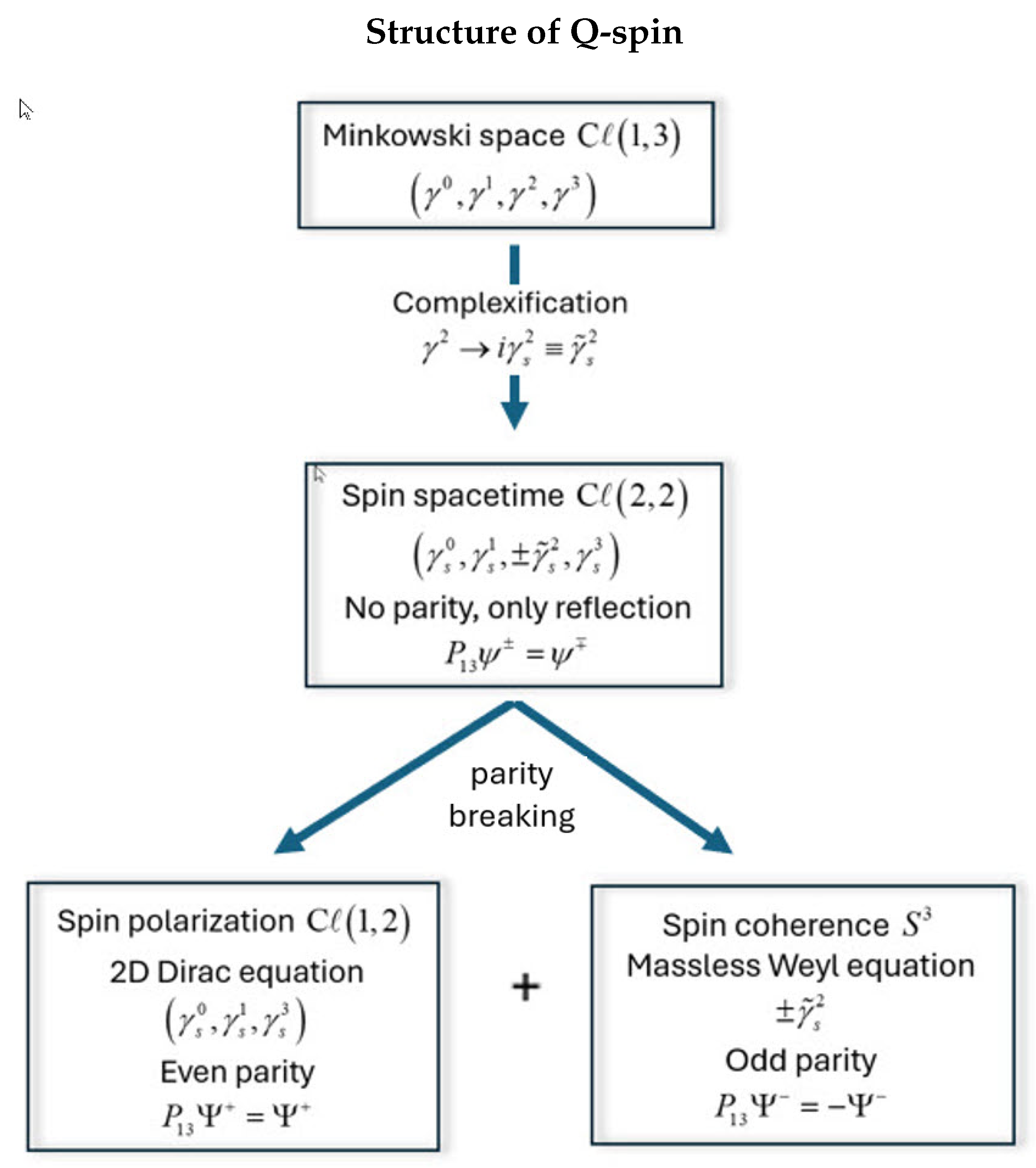
The development of Q-spin from the Dirac field is summarized in Figure 9. Indeed SO is called the split group, [41], and also plays a prominent role in Twistor theory. The non-Hermitian Dirac Equation, (4), displays two reflective states, , without parity. Reflection is a result of changing a right-handed frame to a left-handed one, Figure 4, which is not parity.
We believe at the Big Bang, Nature evolved first with distinct parity which was the dominant and essential property of those epochs. The first microscopic particles were created in an environment that could only create particles with definite parity. We believe that only one such event was needed to create the quantum domain. Definite handedness, unique in the early Universe, has settled down in some places, like on Earth. The distinction is unnecessary macroscopically, but remains still in the microscopic.
When we complexified the Dirac field, we did not expect a 2D spinning disc, a World sheet, [42], nor spin being an anyon, [17]. We did not expect that antimatter production by Dirac’s interpretation would be unnecessary. Our original goal was to find a local way (product state) that accounts for the violation of BI. Once Q-spin was formulated, not only did it resolve the EPR paradox and disproved Bell’s theorem, but also many other problems are resolved, [5].
The ideas presented here are quantum yet provide an alternate view of the microscopic. Important and satisfying features of the macro classical view carry over to the micro. Both are locally real, albeit reality of the microscopic is complex. Equally satisfying is determinism prevails in all dimensions: you measure only what you prepare. The "collapse" of a boson spin to a polarized fermion state, is deterministic. That QM is non-deterministic is a failure of the theory. QM is a mechanics and it is impossible to build structures without determinism. Nature needed three things to build matter: energy, chirality and a rule.
We do not believe that the identical geometric structure of Q-spin and a photon is a coincidence, but rather shows a continuity of properties between microscopic particles. Presently, all particles in the standard model are bosons or fermions, and we suspect those particles should be treated under the quaternion group.
Quaternions, [43], one of the many legacies of Hamilton, [44] are more than mathematical constructs defined on the hypersphere, with four spatial dimensions. Spin is a quaternion which is an element of physical reality with a bivector structure. The unit quaternions coincides with the origin of the Bloch sphere and extends it by adding helicity to each Bloch vector, and these spin either left or right with a constant frequency. Spin is geometrically a vector of helicity, and a bivector of coherence. Nature is described not only by a real disc, in our spacetime, but also the odd parity hypersphere of unit quaternions. Only the 2×2 vector part of spin, , is projected into our spacetime.
Hamilton’s Eureka moment, discovering that rotations in 3D are generated by quaternions in 4D, set the stage for understanding spin. Spin is a quaternion.
Appendix A
We derive Q-spin as a quaternion in the LFF, Eq. (12), by contracting with the polarized field vector, ,
Substitute Equation (15), transform to the LFF using Eq.(16), collect terms and contract using and . Factor out the field quaternion,
Form the quaternion for the initial orientation, ,
Identify the phase,
References
- Sanctuary, B. Quaternion Spin. Mathematics 2024, 12, 1962. [Google Scholar] [CrossRef]
- Sanctuary, B. Spin Helicity and the Disproof of Bell’s Theorem. Quantum Rep. 2024, 6, 436–441. [Google Scholar] [CrossRef]
- Sanctuary, B. C. , Non-local EPR Correlations using Quaternion Spin. Quantum Rep. 2024, 6(3), 409–425. [Google Scholar] [CrossRef]
- Sanctuary, B. The classical origin of intrinsic angular momentum, submitted, 2024.
- Sanctuary, B. Quaternion spin: parity and beta decay, 2025.
- Sanctuary, B. Bell’s theorem and hidden variables, 2025.
- Sanctuary, B. Quantum coherence 2025.
- Sanctuary, B. The singlet state is an approximation. 2025.
- Clauser, J. F., Horne, M. A., Shimony, A., & Holt, R. A. (1969). Proposed experiment to test local hidden-variable theories. Physical review letters, 23(15), 880. [CrossRef]
- Aspect, Alain, Jean Dalibard, and Gérard Roger. “Experimental test of Bell’s inequalities using time-varying analyzers.” Physical review letters 49.25 (1982): 1804.Aspect, Alain (15 October 1976). “Proposed experiment to test the non separability of quantum mechanics”. Physical Review D. 14 (8): 1944–1951. [CrossRef]
- Weihs, G., Jennewein, T., Simon, C., Weinfurter, H., Zeilinger, A. (1998). Violation of Bell’s inequality under strict Einstein locality conditions. Physical Review Letters, 81(23), 5039. [CrossRef]
- Bell, John S. "On the Einstein Podolsky Rosen paradox." Physics Physique Fizika 1.3 (1964): 195.
- Wikipedia contributors. (2024, July 12). Pauli matrices. In Wikipedia, The Free Encyclopedia. Retrieved 12:06, August 15, 2024.
- Dirac, P. A. M. (1928). The quantum theory of the electron. Proceedings of the Royal Society of London. Series A, Containing Papers of a Mathematical and Physical Character, 117(778), 610-624. [CrossRef]
- Penrose, Roger. "Twistor algebra." Journal of Mathematical Physics 8.2 (1967): 345-366. [CrossRef]
- Penrose, Roger. "Solutions of the Zero-Rest-Mass Equations." Journal of Mathematical Physics 10.1 (1969): 38-39. [CrossRef]
- Wilczek, F. (1982). Quantum mechanics of fractional-spin particles. Physical review letters, 49(14), 957. [CrossRef]
- Freedman, M., Kitaev, A., Larsen, M., and Wang, Z. (2003). Topological quantum computation. Bulletin of the American Mathematical Society, 40(1), 31-38.
- Kauffman, L. H., and Lomonaco, S. J. (2004). Braiding operators are universal quantum gates. New Journal of Physics, 6(1), 134. [CrossRef]
- Hestenes, D., and Sobczyk, G. (2012). Clifford algebra to geometric calculus: a unified language for mathematics and physics (Vol. 5). Springer Science and Business Media.
- Doran, C., Lasenby, J., (2003). Geometric algebra for physicists. Cambridge University Press.
- Peskin, M.; Schroeder, D.V. An Introduction To Quantum Field Theory; Frontiers in Physics: Boulder, CO, USA, 1995.
- Edmonds, A. R. (1957). Angular Momentum in Quantum Mechanics. Princeton, New Jersey: Princeton University Press. ISBN 978-0-691-07912-7.
- Coope, J. A. R., Snider, R. F., and McCourt, F. R. (1965). Irreducible cartesian tensors. The Journal of Chemical Physics, 43(7), 2269-2275. [CrossRef]
- Coope, J. A. R., and Snider, R. F. (1970). Irreducible cartesian tensors. II. General formulation. Journal of Mathematical Physics, 11(3), 1003-1017. [CrossRef]
- Coope, J. A. R. (1970). Irreducible Cartesian Tensors. III. Clebsch-Gordan Reduction. Journal of Mathematical Physics, 11(5), 1591-1612. [CrossRef]
- Coope, J. A. R., Sanctuary, B. C., and Beenakker, J. J. M. (1975). The influence of nuclear spins on the transport properties of molecular gases and application to HD. Physica A: Statistical Mechanics and its Applications, 79(2), 129-170. [CrossRef]
- Snider, R. F. (2017). Irreducible Cartesian Tensors (Vol. 43). Walter de Gruyter GmbH and Co KG.
- Bell, J. S. (1987). Speakable and unspeakable in quantum mechanics Cambridge University Press. New York, Bell’s quote is on page 65.
- Tsirel’son, B. S. (1987). Quantum analogues of the Bell inequalities. The case of two spatially separated domains. Journal of Soviet Mathematics, 36, 557–570. [CrossRef]
- Dirac, P. A. M. (1930). "A Theory of Electrons and Protons". Proc. R. Soc. Lond. A. 126 (801): 360–365. [CrossRef]
- Conrad, J. M., & Shaevitz, M. H. (2018). Sterile neutrinos: An introduction to experiments. Adv. Ser. Direct. High Energy Phys, 28, 391-442.
- Baryon Asymmetry. In Wikipedia. Available online: https://en.wikipedia.org/wiki/Baryon_asymmetry (accessed on 6 April 2024).
- Riotto, A., & Trodden, M. (1999). Recent progress in Baryogenisis. Annual Review of Nuclear and Particle Science, 49(1), 35-75.
- Steigman, G. (2007). "Primordial Nucleosynthesis in the Precision Cosmology Era". Annual Review of Nuclear and Particle Science, 57: 463-491. [CrossRef]
- Ade, P. A. R. et al. (Planck Collaboration) (2016). "Planck 2015 results. XIII. Cosmological parameters". Astronomy & Astrophysics, 594, A13.
- Ahmadi, M.; Alves, B.X.R.; Baker, C.J.; Bertsche, W.; Butler, E.; Capra, A.; Carruth, C.; Cesar, C.L.; Charlton, M.; Cohen, S.; et al. Observation of the 1S–2S transition in trapped antihydrogen. Nature 2017, 541, 506–510. [Google Scholar] [CrossRef] [PubMed]
- Anderson, E. K., Baker, C. J., Bertsche, W., Bhatt, N. M., Bonomi, G., Capra, A., ... and Wurtele, J. S. (2023). Observation of the effect of gravity on the motion of antimatter. Nature, 621(7980), 716-722. [CrossRef]
- Wick, David. The Infamous Boundary: Seven decades of heresy in quantum physics. Springer Science and Business Media, 2012.
- Wu, C. S., Ambler, E., Hayward, R. W., Hoppes, D. D., and Hudson, R. P. (1957). Experimental test of parity conservation in beta decay. Physical review, 105(4), 1413. [CrossRef]
- Jain, A. Unitary irreducible representations of SO (2, 2) and SO (3, 2).
- Maldacena, J., Susskind, L. (2013). Cool horizons for entangled black holes. Fortschritte der Physik, 61(9), 781-811. [CrossRef]
- Snygg, J. (1997). Clifford Algebra: A Computational Tool for Physicists. Oxford University Press on Demand.
- Gsponer, A., Hurni, J. P. (2002). The physical heritage of Sir WR Hamilton. arXiv preprint math-ph/0201058.
Figure 1.
A single spin is oriented in spin spacetime by the BFF basis vectors , which spin about the axis so that in Minkowski space, with the basis vectors , only a smeared-out image of the precessing spin is projected. The lower right insert contrasts Dirac spin and Q-spin, which is displayed as the resonance formed from coupling the N and E axes.
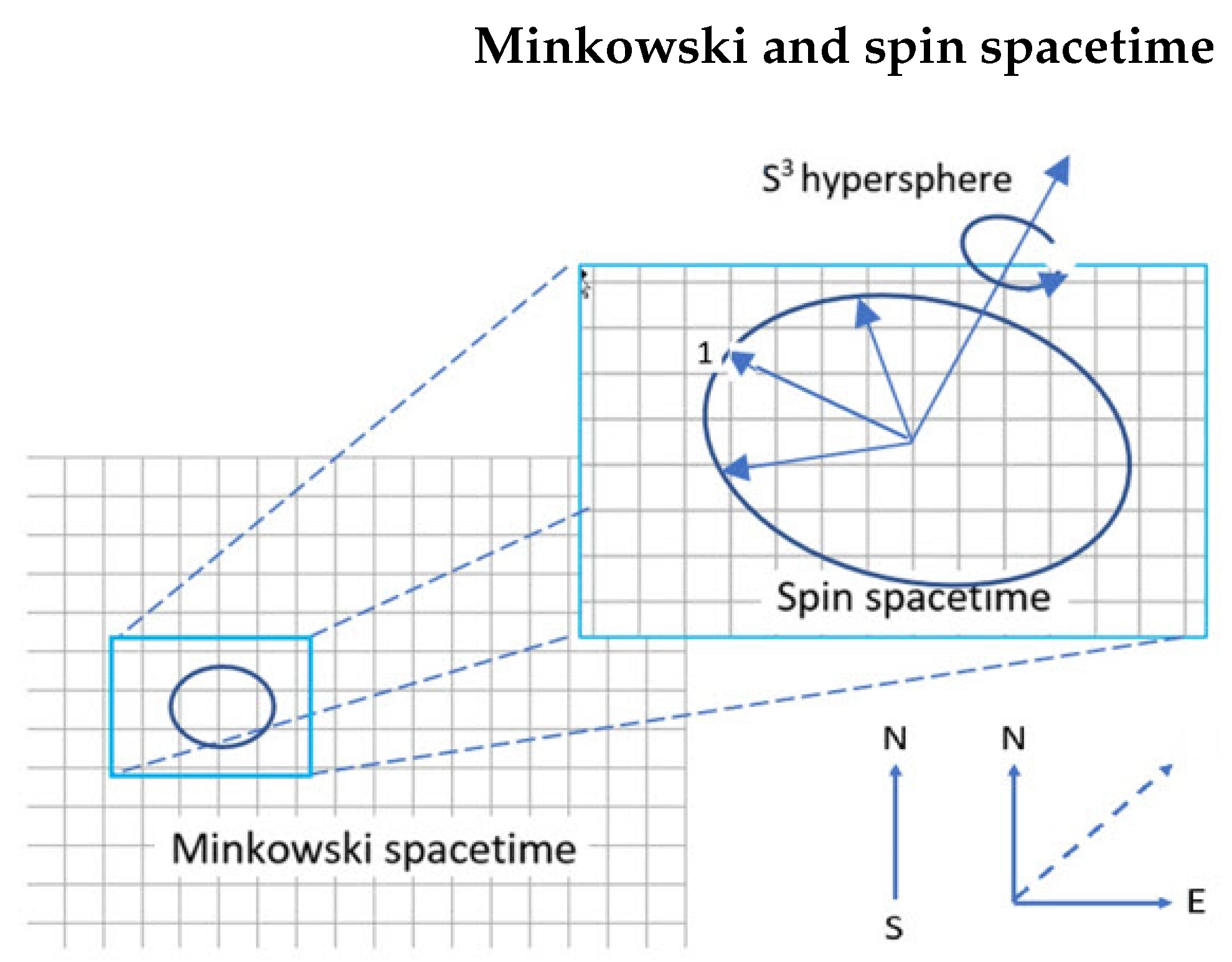
Figure 2.
Classical and quantum spin: Top: A classical model for Q-spin with two orthogonal massive axes, 1 and 3, spun around the massless 2 axis with frequencies up to the relativistic limit, . Bottom: two orthogonal spin- polarization vectors, and , perpendicular to the direction of linear momentum, Y. The helicity is in the direction of propagation, , and spins right or left. The two spin- vectors, and , couple to give a composite boson, , of magnitude 1.
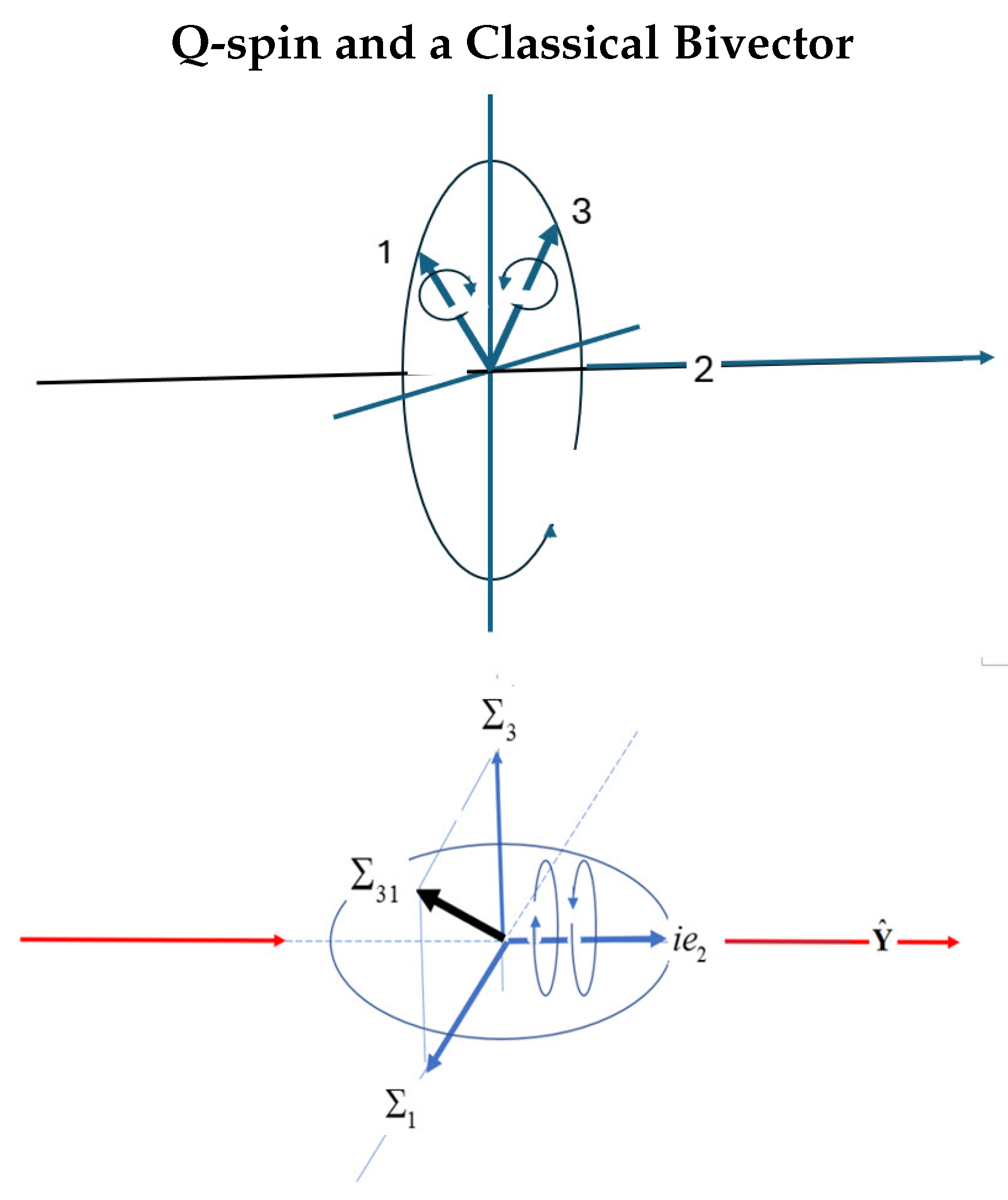
Figure 3.
The Classical domain: In the rotating frame of the disc. Showing the left and right hands of Nature. The angle, , between the axes, 1 and 3, and their angular momentum cones increases as the precession frequency increases. A mirror plane bisects the 1 and 3 axes. The centrifugal force from 2 is directed along the bisector, 13.
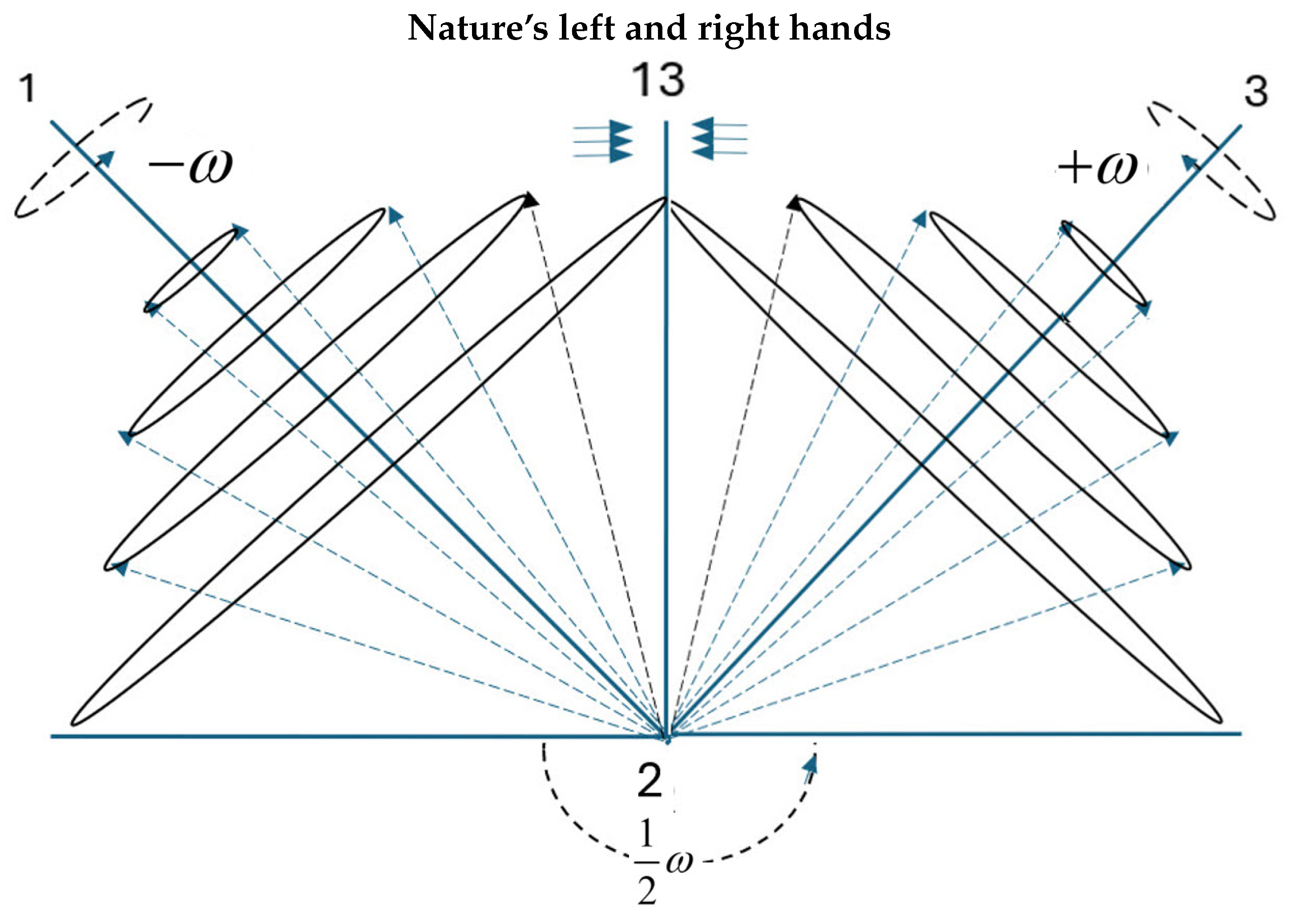
Figure 4.
The mirror or reflective states of a Q-spin with, say, on the right and on the left. Note that adding these states is independent of and subtracting them is independent of and . This separates polarization from coherence, leading to a symmetry breaking between them. Imagine being inside the mirror plane, allowing you to see both left and right frames simultaneously. If you added them, you see matter; if you subtract them, you see torques.
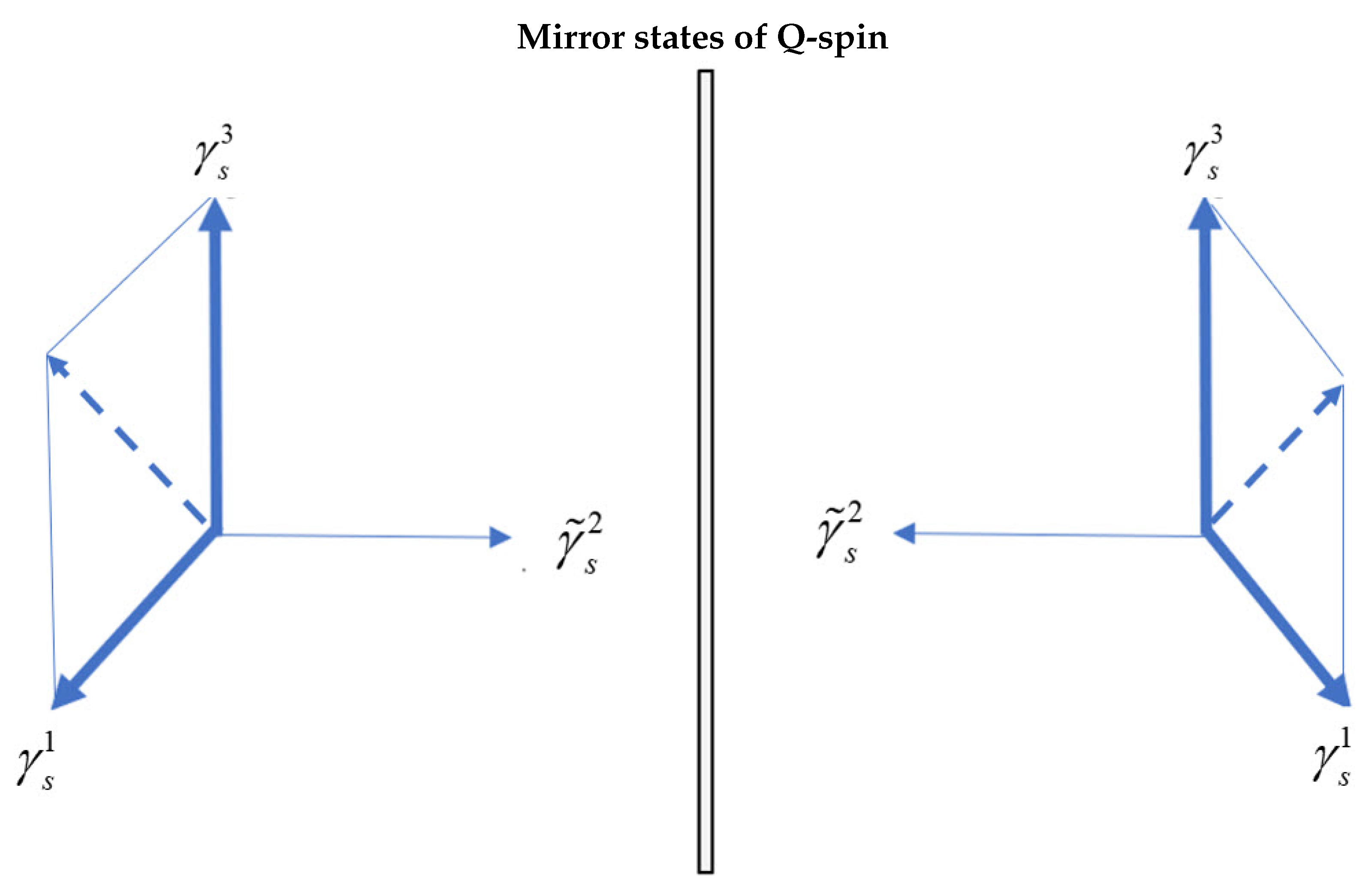
Figure 5.
The boson deterministically choose chirality. The longer arrow denotes the direction of the polarizing field. Top: The two mirror states in free flight, and , couple to give a boson spin-1. Left and right: The fermionic axis closer to the field axis aligns, and the boson decouples. These two panels do not indicate two particles but one Q-spin depicted with one for the other axis aligned with the field. Bottom: When the boson spin is close to the field, it initially precesses as a spin-1 without decoupling.
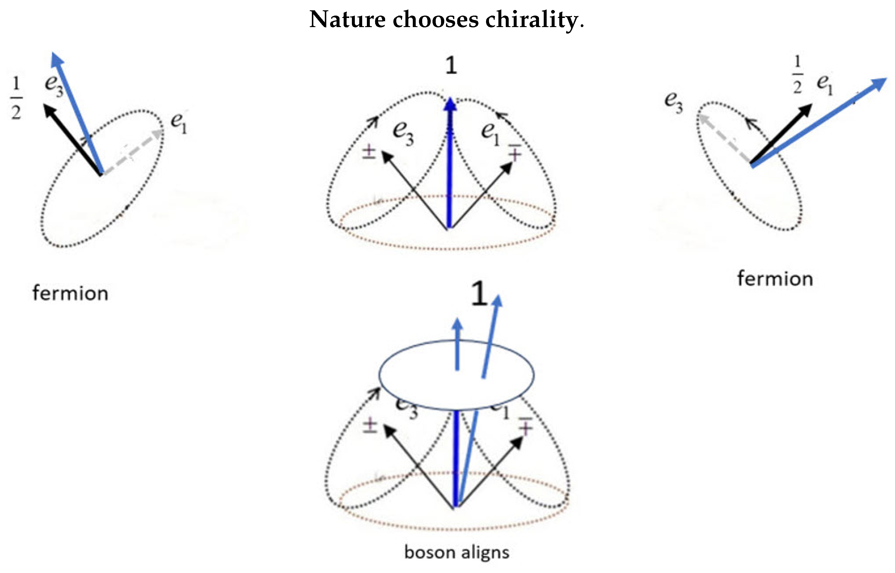
Figure 6.
Parentage Scheme. The number of linearly independent irreducible representations of weight ℓ in a spinor of order p, [28].
Figure 6.
Parentage Scheme. The number of linearly independent irreducible representations of weight ℓ in a spinor of order p, [28].
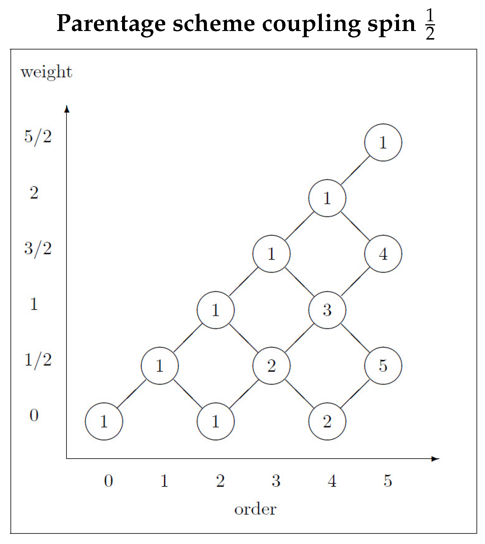
Figure 7.
Plotting EPR correlation versus the angle difference . The points give the results of the simulation. The CHSH values are listed and the full correlation is the sum of polarization, (the triangle) and the coherence, (the mustache). Note the hardly discernible residual polarization correlation along the horizontal axis, which shows the contribution extracted from the polarization, .
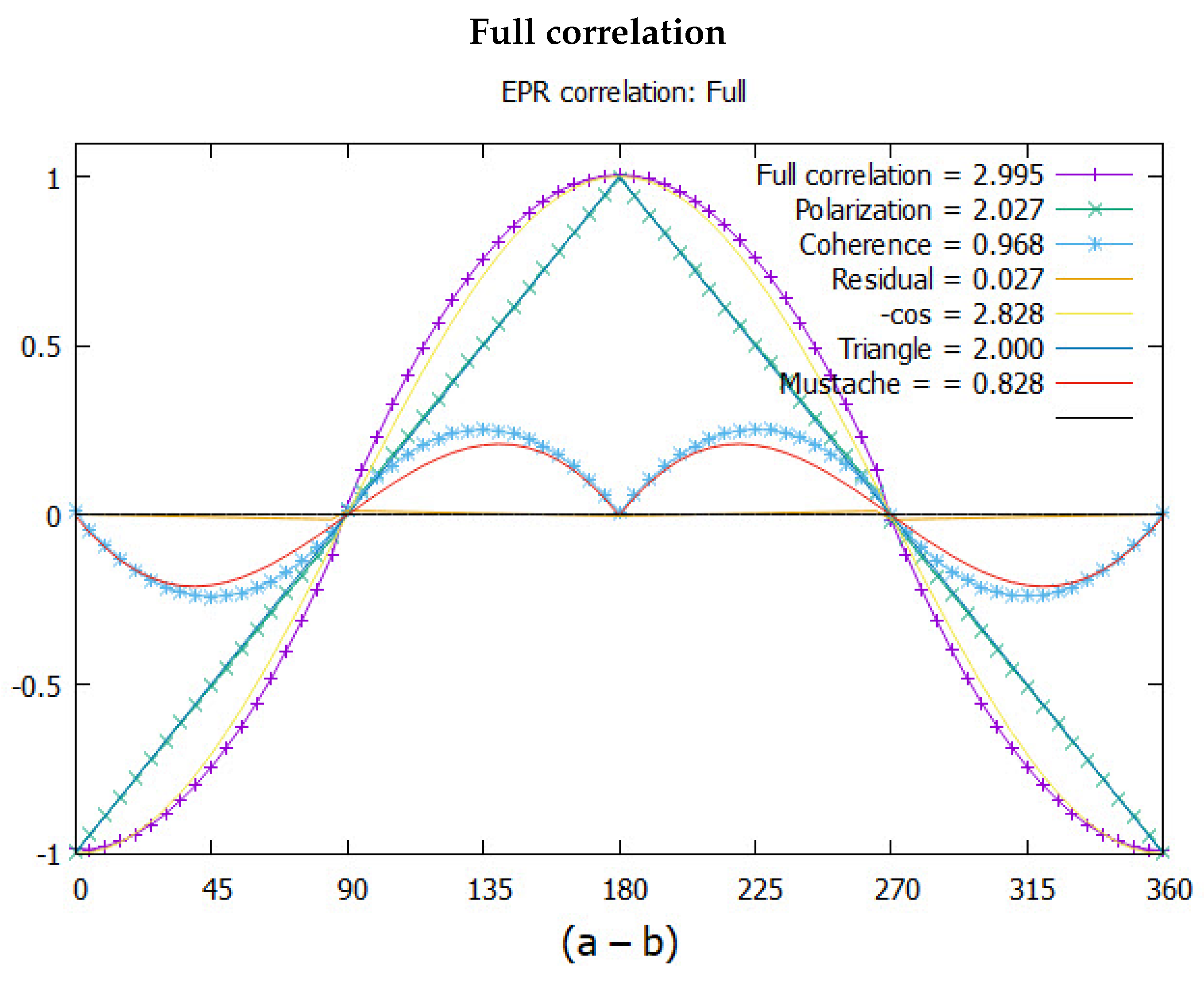
Figure 8.
Under charge conjugation, the axes and the precessions reverse with no physical difference.
Figure 8.
Under charge conjugation, the axes and the precessions reverse with no physical difference.
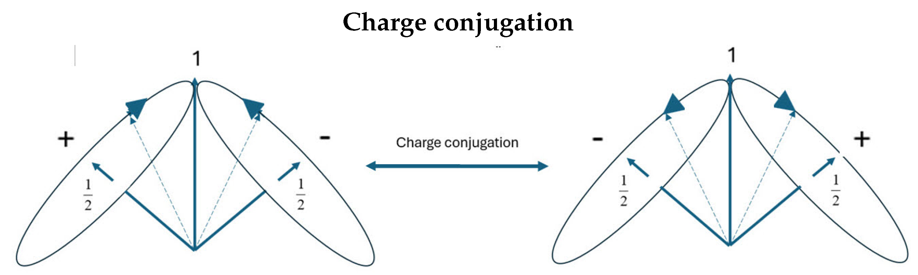
Figure 9.
The structure and separation of spin spacetime into complementary spaces of polarization and coherent helicity.
Figure 9.
The structure and separation of spin spacetime into complementary spaces of polarization and coherent helicity.
Disclaimer/Publisher’s Note: The statements, opinions and data contained in all publications are solely those of the individual author(s) and contributor(s) and not of MDPI and/or the editor(s). MDPI and/or the editor(s) disclaim responsibility for any injury to people or property resulting from any ideas, methods, instructions or products referred to in the content. |
© 2024 by the authors. Licensee MDPI, Basel, Switzerland. This article is an open access article distributed under the terms and conditions of the Creative Commons Attribution (CC BY) license (http://creativecommons.org/licenses/by/4.0/).
Copyright: This open access article is published under a Creative Commons CC BY 4.0 license, which permit the free download, distribution, and reuse, provided that the author and preprint are cited in any reuse.


