
Submitted:
27 December 2024
Posted:
30 December 2024
You are already at the latest version
Abstract
Accurate vegetation mapping is essential to enhance understanding of important ecosystem processes such as fire behaviour, nutrient cycling, plant community composition and mega-herbivore population dynamics in African savannahs.The inherent heterogeneity of savannah landscapes however creates significant challenges for accurate discrimination of vegetation components. Recent studies based on the use of optical remote sensing data favour very high spatial resolution (VHR) multi-spectral imagery for dealing with this challenge. However, such data are costly for use in operational management. Planet Labs, through Norway’s International Climate and Forests Initiative (NICFI) in partnership with Kongsberger Satellite Services (KSAT) and Airbus, now grant free access to high-resolution, analysis-ready mosaics of Planet imagery over the tropics, with great potential for fine-scale vegetation mapping. However, the spectral characteristics of these data are limited, with little knowledge of their ability to resolve the spectral similarity of heterogeneous savannah vegetation components. In parallel, Sentinel-2 samples a relatively high number of spectral bands, but has relatively coarse spatial resolution for dealing with the high spatial heterogeneity in African savannah landscapes. We test the hypothesis that fusing Sentinel-2 with Planet imagery leverages their spectral and spatial advantages to enhance accurate discrimination of savannah vegetation types. To achieve this, Principal Component and Gram-Schmidt transformations were compared for image fusion via pan-sharpening, where the Gram-Schmidt approach proved superior. Using this approach, we fused Sentinel-2 and Planet images and compared the three datasets (i.e. Sentinel-2, Planet and Fused images) augmented with two spectral indices and three Haralick texture features in a multi-layer perceptron neural network classification within a test site in the Lower Sabie region of Kruger National Park, South Africa. Overall, the Fused image achieved the best and most precise classification accuracy metrics (weighted F-score: 0.87±0.012) compared to Sentinel-2 (weighted F-score: 0.85±0.034) and Planet imagery (weighted F-score: 0.85±0.017). A comparison of classifications showed loss in spatial detail when using Sentinel-2 (at 10 meters spatial resolution), yet similar thematic details for vegetation classes across all three datasets. Our findings highlight the utility of Sentinel-2 and the Planet-NICFI mosaics in a heterogeneous savannah landscape, while setting a foundation for cost-effective and accurate high spatial resolution monitoring of savannah ecosystem.
Keywords:
Image fusion
; Pan-sharpening
; Gram-Schmidt transformation
; Planet/NICFI imagery
; Sentinel-2
; Multilayer perceptron
; African savannah
1. Introduction
Satellite remote sensing technology offers unparalleled opportunities for cost-effective spatio-temporal quantification and analysis of land cover distributions. The availability of open-access satellite imagery - such as those from the Landsat [1] and Sentinel-2 [2] missions - and accompanying image processing frameworks have expedited land cover classification workflows with enhanced accuracy. Some regions and biomes such as forests have been studied extensively, partly due to standardized classification workflows and methodology. Conversely, savannahs in particular have received relatively little attention and remain a major source of uncertainty in land cover products globally [3,4]. Recent research has focused on optimizing savannah land cover characterization mainly through the use of multi-source satellite images [5,6,7], improved image resolution and benchmarking of classification methods [8,9]. However, the inherent high spatial heterogeneity in savannah landscapes and spectral similarity between different vegetation components still present considerable challenges for accurate discrimination of vegetation components.
To deal with the spectral confusion among different vegetation components, integration of multi-season image acquisitions [6,7] and the use of images from the dry season [10,11] have been proven to capitalize on phenological differences and increase discrimination space among spectrally similar vegetation components. The use of radar imagery or LiDAR has also been useful to discriminate between vegetation components by including structural information, e.g. grass vs woody vegetation [6,12]. Yet, classification accuracy is influenced significantly by image spatial resolution (e.g. see [13]), where medium resolution imagery is impaired by pixel mixing under spatially heterogeneous savannah landscape conditions, restricting their success to rather general and continuously distributed target land cover classes. Current research favours very high spatial resolution (VHR, ≤ 5m) satellite imagery for dealing successfully with these challenges (e.g. [8,9,13]). For example, Marston et al. [13] showed that VHR IKONOS, Quickbird and WorldView-2 imagery can discriminate more savannah vegetation classes and at higher accuracies (Overal Accuracy (OA): ) than medium resolution imagery (OA: ). In a related study, Awuah et al. [9] demonstrated the potential of WorldView-3 imagery for mapping plant functional types in mesic and semiarid southern African savannahs with very high accuracies (F-score: ).
While VHR satellite images are ideal for heterogeneous savannah landscapes, such high resolution data are costly for operational monitoring of savannah vegetation and other land cover dynamics. A recent partnership involving Norway’s International Climate and Forests Initiative (NICFI), Kongsberger Satellite Services (KSAT), Planet Labs and Airbus now grant free access to high-resolution, analysis-ready mosaics of Planet imagery over tropical regions [14]. This promises new opportunities for rapid and cost-effective vegetation monitoring at high spatial scales. High spatial resolution Planet imagery has been proven successful for vegetation mapping, particularly in forest [15] and agricultural [16] landscapes. However, the spectral characteristics are limited and have shown less success in resolving the spectral similarity of different savannah vegetation components [17]. Alternatively, open-access medium resolution satellite sensors such as Landsat Operational Land Imager (OLI) and Sentinel-2 sample relatively high numbers of spectral bands, potentially useful for mapping vegetation in African savannah landscapes [17].
Generally, pixel-based classification tends to perform better when image spatial resolution is relatively coarse [18]. However, the prevalence of high within-class spectral variance in VHR imagery increases misclassification and can create a ’salt-and-pepper’ effect when using pixel-based classification [8,19]. Alternatively, object-based image analysis (OBIA) aggregates pixels through the process of segmentation, creating contiguous groups of pixels with high spectral homogeneity known as image objects [20]. OBIA is widely recommended for the classification of VHR imagery [20,21], particularly in heterogeneous landscapes [8,22,23]. In a specific African savannah classification using WorldView-2 imagery, Kaszta et al. [8] showed that OBIA had a significantly higher accuracy across all seasons and different machine learning frameworks relative to pixel-based classification.
In this study, we leverage both the high number of spectral bands of Sentinel-2 imagery and high spatial resolution of Planet imagery, integrating these two data sources for object-based classification of different vegetation components in a heterogeneous southern African savannah landscape. The study explores pixel-level image fusion approaches for integrating Sentinel-2 and Planet imagery. Compared with other popular image fusion techniques such as the Intensity-Hue-Saturation transform [24] and Principal Component transform [25], Gram-Schmidt transformation [26] has been found to be fast and generates fused images with high spatial detail while preserving spectral integrity [26,27]. Rokni et al. [28] compared Modified Intensity-Hue-Saturation, High Pass Filter, Gram Schmidt and Wavelet-PC (Principal Components) techniques for fusion of multi-temporal Landsat Enhanced Thematic Mapper Plus (ETM+) 2000 band 8 (15 m) and Landsat Thematic Mapper (TM) 2010 multispectral (30 m) images towards surface water detection. The study [28] found the Gram-Schmidt image fusion technique to produce better outcomes both in terms of resulting image quality and classification. Further, the potential of Gram-Schmidt transformation for multi-sensor image fusion has been successfully demonstrated, with examples including pixel-level fusion of Unoccupied Aerial Vehicle (UAV) derived VHR aerial imagery with Landsat-8 OLI [29] and Sentinel-2 imagery [27] in agricultural landscapes. The performance of the different pan-sharpening approaches has not been demonstrated in heterogeneous savannah landscape. Therefore, this study compares the Gram-Schmidt and Principal Component transformations in the fusion of Sentinel-2 and Planet imagery. The Principal Component (PC) method was selected as the alternative to Gram-Schmidt in this study for two main reasons: (i) it is widely recognized and frequently used in image fusion studies, providing a robust baseline for comparison with newer techniques; and (ii) its simpler implementation and computational efficiency make it a practical option for many applications. While methods such as High Pass Filter or Modified Intensity-Hue-Saturation have demonstrated their utility in specific contexts, the PC method serves as a representative benchmark due to its historical prominence and general applicability in remote sensing. This choice allows us to highlight the superiority of Gram-Schmidt in a heterogeneous savannah landscape context while using a well-understood and widely applied alternative for comparison.
We hypothesize that fusion of Sentinel-2 images with Planet imagery leverages their spectral and spatial advantages and enhances discrimination of savannah vegetation types leading to better classification accuracies. To test this hypothesis, we (i) first compare the performance of Gram-Schmidt and Principal Component methods for image fusion to select the best fusion outcome; and (ii) compare the original Sentinel-2 and Planet imagery with their fused version (i.e. Sentinel-2 + Planet imagery) for discriminating savannah land cover types.
2. Materials and Methods
2.1. Study Area
The study site is located in Kruger National Park (KNP), South Africa (Figure 1). The test area covers 1220 ha extending over portions of the Sabie River catchment and encompassing the Nkhulu exclosure within the Lower Sabie region of KNP. Mesic savannah landscape conditions prevail within the area with mean rainfall ranging between 600 mm and 700 mm annually [30]. The site has underlying granite geology and is dotted with sodic sites often occurring at the footslopes of catenas, which are known to have high soil sodium content. Sodic sites provide dietary sodium supplement and thus, attract and concentrate grazers on these parts of the savannah landscape, making them significant drivers in grazing lawn formation [31]. Vegetation within the study site is predominantly composed of thorn thickets (e.g., Acacia robusta), silver clusterleaf (Terminalia sericea) and sour grasses (Hyparrhenia filipendula) [32]. Apart from the abiotic determinants of vegetation type distribution in KNP, the presence of high population densities of grazers (e.g. buffalo, blue wildebeest, zebra, hippo), browsers (e.g. giraffe and kudu), and mixed feeders (e.g. impala and elephant) exert significant impact on vegetation structure [33].
2.2. Land Cover Classification Nomenclature
Three vegetation classes were identified based on structure. These included (i) woody; (ii) bunch grass; and (iii) grazing lawns. The target vegetation classes provided for a more objective in-situ and image-based discrimination of vegetation components during reference data collection. Trees and shrubs in savannah landscapes are structurally complex to discriminate due to disturbance adaptations such as multiple stems, toppled, leaning among others [34]. These were thus grouped under a single woody category. Grazing lawns were identified as short grass patches with height ≤ 20 cm, often with sparse distribution and stoloniferous growth behavior, while grass patches > 20 cm in height were categorized as bunch grasses. In addition to the vegetation classes, water bodies, bare soil and built-up were considered, totaling six land cover classes used for image classification. A summary of land cover classification nomenclature is provided in Table 1.
2.3. Reference Data
Field surveys were conducted in the dry season of 2019 between June 27 and July 21. A total of 111 point locations systematically distributed within a 200 m buffer and beyond 100 m distance from access roads were visited. Site descriptions of surrounding vegetation patches and other land cover were recorded together with cardinal direction photographs (north, east, south, west) to aid reference data generation. Data from in-situ reference locations were supplemented with 497 randomly distributed points within the bounds of the image footprint, with minimum spatial separation distance of 100 m to minimize autocorrelation. Overall, 3398 polygons were manually digitized from spectrally homogeneous areas within 100 m radius of sample point locations based on knowledge from field visits. Digitized polygon objects have been shown to produce the most accurate classification outcomes compared to other approaches for extracting training data such as points, lines and segmentation objects [35,36]. Reference polygons were labeled according to the different land cover categories (Table 1) via visual interpretation of very high-resolution WorldView-3 imagery and Google Earth satellite scenes with the same temporal window (June/July 2019), augmented by field photos and descriptions of land cover.
2.4. Remote Sensing Data and Preprocessing
The remote sensing data used in this study comprise cloud-free Sentinel-2A and Planet images taken during the dry season. Image acquisition dates coincide with the period of in-situ land cover surveys (see Section 2.3), to allow consistent classification and accuracy assessment. The Sentinel-2A and Planet images were co-registered to the WorldView-3 image used in reference polygon creation to allow spatial consistency during the extraction of reference pixels and comparison of classification results.
Sentinel-2 is a multi-spectral satellite imaging mission designed and operated by the European Space Agency (ESA) as part of the Global Monitoring for Environment and Security (GMES) initiative [2]. It includes a constellation of two polar-orbiting satellites (Sentinel-2A and Sentinel-2B), phased at 180o to each other in a sun-synchronous orbit. The integration of two satellites provides a 5-day revisit frequency at the equator with a 290 km swath [37]. The mission features a Multi Spectral Instrument (MSI) which samples 13 spectral bands ranging from visible and near infrared to shortwave infrared portions of the electromagnetic spectrum. The spatial resolution varies depending on the spectral bands: four bands at 10 m, six bands at 20 m and three bands at 60 m. Sentinel-2 images are freely available for download from a number of open-access portals, but primarily served on the Copernicus Open Access Hub website (https://scihub.copernicus.eu/). In this study, the Sentinel-2A image was acquired through the Google Earth Engine platform [38]. Images were acquired between May and June 2019 and had been pre-processed to surface reflectance using the Sen2Cor module [39] as Level-2A products, from which a median composite was created. Overall, 10 spectral bands were used covering the visible and near infrared (NIR) channels at 10 m spatial resolution and the red edge (RE) and shortwave infrared (SWIR) bands at 20 m spatial resolution. The RE and SWIR bands were resampled to 10 m to ensure consistency with the visible and NIR bands.
The Planet image is part of the open-access analysis-ready (ARD) satellite image data over tropical regions. The archive features bi-annual mosaics between December 2015 and August 2020 and monthly mosaics available from September 2020 onward. Access to this VHR ARD satellite imagery was made available through a partnership between NICFI, KSAT, Planet Labs and Airbus (operational on October 22, 2020), intended to support efforts against tropical deforestation. The mosaics are constructed using best pixels from daily Planet imagery processed to surface reflectance either as three-band (Blue, Green and Red) or four-band (Blue, Green, Red and Near Infrared) image composites. In this study, the four-band ARD composite covering June 2019 to December 2019, with spatial resolution of 4.77 m per pixel was used.
2.5. Multi-sensor Image Fusion
Pixel-level image fusion of Sentinel-2A and Planet imagery was achieved via pan-sharpening using Gram-Schmidt transformation [26] and Principal Component transformation [25]. In this study, the higher spatial resolution panchromatic band was simulated from the Planet image as the mean of all four bands. To fuse the simulated panchromatic band with the lower spatial resolution Sentinel-2A image, first, a lower spatial resolution panchromatic band is simulated from the Sentinel-2A image. Second, Gram-Schmidt and Principal Component transformations are separately performed on the simulated lower spatial resolution panchromatic band and the plurality of the Sentinel-2A bands, with the lower spatial resolution panchromatic band employed as the first band in the transformation process. Third, the statistics (mean and standard deviation) of the higher spatial resolution panchromatic image are adjusted to match the statistics of the first output band from the Gram-Schmidt and Principal Component transformations using histogram matching. Fourth, the first transform band is replaced with the adjusted higher spatial resolution panchromatic band to produce a new set of Gram-Schmidt and Principal Component transform bands. Finally, an inverse transformation is performed to return the new set of transform bands into a higher spatial resolution multi-spectral band space. The best output from both image transformation methods was selected for further processing. Figure 2 shows a summary of the analysis workflow used in this study.
2.6. Image Quality Assessment
The image fusion approach was evaluated to ascertain improvement in spatial resolution and preservation of image spectral characteristics. First the fused image was visually compared to the original images (Sentinel-2A and Planet imagery) to compare the spatial details resolved. Second, two statistical metrics were computed to evaluate the preservation of image spectra. This included: (i) correlation coefficient (CC) between the original Sentinel-2A image bands and the equivalent bands from the fused image (CC ranges between -1 and 1, where values closer to 1 or -1 show increasing positive or negative correspondence between band pairs); and (ii) structural similarity index (SSIM) [40] comparing the multi-spectral Sentinel-2A and fused images. SSIM combines luminance, contrast and structure, and was calculated with a moving 9 x 9 pixel neighbourhood. SSIM computation using a moving window over both images helps to capture spatial variation and ultimately leads to better estimates of (dis)similarity between images [41]. The 9 x 9 pixel neighborhood was deemed appropriate to cover enough spatial variation while minimizing computational cost. The SSIM values range between -1 and 1, and only equals 1 if the two images are identical. CC and SSIM were calculated using Equations 1 and 2
where is covariance for band pairs () and and are standard deviations for band x and y respectively.
where and are mean intensities, is covariance, and are standard deviations, and are constants for luminance and contrast comparisons respectively, used to stabilize the equation in the presence of weak denominators [40]. In this case x and y represent the original Sentinel-2 image and the fused image respectively. The output from the best performing fusion approach (i.e., between Gram-Schmidt and Principal Component pan-sharpening) was selected for further processing and classification.
2.7. Image Segmentation
Image segmentation was performed on all image datasets (i.e. Sentinel-2, Planet and fused images). This involved the computation of a gradient image from the original input image bands using a Sobel edge detection method [42], followed by a watershed transform [43]. The watershed transform algorithm is modeled after the hydrologic watershed concept, with a landscape composed of basins. Basins fill up with water starting at the lowest points until flooded, and dams are built at the meeting point of water coming from different basins. The landscape is thus divided into regions (watersheds) separated by dams (watershed lines). Similarly, the watershed transform algorithm considers the gradient image as a topological surface where dark pixels represent lower elevation (minimum). The algorithm sorts the gradient image pixels by increasing intensity values and ’floods’ the image starting with the lowest gradient values (uniform portions of object) to the highest gradient values (object edges). The results is a segmentation image partitioned into regions with similar pixel intensities where each region is assigned the mean intensity value. A Full Lambda algorithm, which merges smaller segments within larger, textured areas, was used to minimize over-segmentation [44].
2.8. Feature Extraction
In addition to the original segmentation image bands, two spectral indices and three Haralick textural image features were calculated for all datasets in order to enhance land cover discrimination space. The spectral indices included the Global Environmental Monitoring Index (GEMI) [45] (Equation 3) and Modified Soil Adjusted Vegetation Index-2 (MSAVI2) [46] (Equation 4) while Mean (Equation 5), Variance (Equation 6) and Sum Average (Equation 7) constituted the Haralick texture features [47]. The spectral indices and texture features were selected following results from a related study [9], where they ranked amongst the most important features in savannah plant functional types (PFTs) classification across different machine learning models. The Haralick texture features were calculated on the NIR band based on Gray Level Co-occurrence Matrix (GLCM) [47] using a 3x3 moving window, at an offset distance of 1 pixel in all directions (, , and ) [6,48].
where and R are near infrared and red bands respectively.
where G is the number of distinct gray levels, i and j are co-occurring intensity values, is the marginal probability of the entry obtained by summing rows of the GLCM, is mean of row sums of the GLCM and represents GLCM sum distribution.
2.9. Image Classification and Accuracy Assessment
The segmented image composed of original bands, spectral indices and texture features (for each dataset) was normalized by subtracting the mean and dividing by its standard deviation for each image band to minimize bias during algorithm training and image classification. The normalized segmented image served as input in a deep neural network classification model using Multilayer Perceptron (MLP) network architecture. MLP is a simple feed-forward deep learning model trained via back-propagation [49]. MLP neural networks excel at handling complex non-linear classification tasks [50,51] making them ideal for application in a highly heterogeneous savannah landscape [9]. Three hidden layers with 64, 32 and 8 neurons for the first, second and third hidden layers respectively were found to yield optimal accuracy after initial experimentation. Dropout layers [52] were used between the dense layers, which randomly neglected 20% of weights in order to reduce overfitting and improve generalization error. The model was compiled using a constant learning rate of 0.001 with Adams optimizer [53] and a categorical cross-entropy loss function.
Accuracies of classification outputs were assessed using a confusion matrix [54] from which a combination of aggregate and individual class based metrics were calculated. The accuracy metrics included precision (Equation 8), recall (Equation 9) and F-score (Equation 10).
where tp, fp and fn represent the number of true positive, false positive, true negative and false negative cases, respectively.
A stratified 10-fold cross-validation approach was adopted during accuracy assessment. Compared to the split-sample approach, cross-validation is more robust due to the availability of multiple metrics and minimizes the risk of chance results while providing for a more efficient use of limited data. Cross-validation accuracy results (i.e. using F-scores) from the individual datasets (i.e. Sentinel-2A, Planet and Fused) were compared using the Friedman test [55,56] to determine the significance (at ) of accuracy differences. The Friedman test is a non-parametric test for comparing three or more treatment scenarios [57] by assigning ranks to treatments separately for each data point. In the case of this study, the Friedman test ranks F-scores from each iteration of cross-validation across all datasets (i.e. Sentinel-2A, Planet and Fused) and compares the average ranks under the null hypothesis that all datasets have equal average ranks. Assuming is the rank for the j-th of k datasets on the i-th out of N cross-validation scores, the average rank is . The Friedman statistic is calculated using Equation 11 [57].
The Friedman test follows a chi-square distribution with k-1 degrees of freedom. We used the Nemenyi test [58] for post-hoc analysis in cases where there were significant differences in accuracy scores among the three datasets used. Similar to the Tukey test for Analysis of Variance (ANOVA), Nemenyi test is used to compare all groups (i.e. datasets in the case of this study) to each other. Two groups are significantly different if the difference between their average ranks is greater than a critical difference (CD) calculated using Equation 12.
where represents a critical value from the studentized range statistic divided by [57].
2.10. Feature Importance Estimation
The contribution of individual image features to classification accuracy was assessed through permutation [59]. This was achieved by randomly shuffling each image feature to determine importance estimates as weights based on degree of reduction in classification accuracy score.
3. Results
3.1. Image Fusion Accuracy
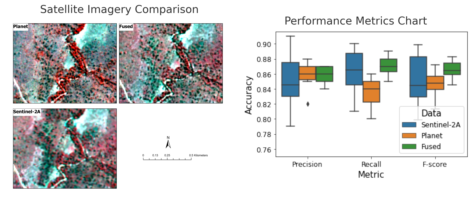
Pixel-level image fusion resulted in the creation of a new dataset (Fused image), which retained both the spectral characteristics of Sentinel-2A and the high spatial resolution from Planet data. Figure 3 shows an example visual comparison of spatial details resolved by all three datasets (i.e. Sentinel-2A, Planet and Fused images). As expected, the Sentinel-2A image at 10 m spatial resolution has a higher level of pixelation at the same visualization scale as Planet and Fused images due to its relatively coarse resolution. Further, land cover features are less distinctly resolved, with high prevalence of pixel mixing in some instances. For example, the sparsely distributed and smaller-sized woody vegetation components become mixed-up with the background grassy vegetation and are indistinguishable (for crowns < 10 m) in the Sentinel-2A image compared to the Fused and Planet images (Figure 3). By contrast, the Fused image is finer and shows similar spatial detail as the high resolution Planet data. At 4.7 m spatial resolution, this enables easy identification of objects that are not recognizable in the Sentinel-2A image while retaining the multi-spectral information from Sentinel-2A. Additionally, the spatial boundaries between different land cover types are better distinguished at the spatial resolution of the Fused and Planet images compared to Sentinel-2A (Figure 3), which could have important consequences for accurate land cover classification.
Apart from the enhanced image spatial resolution, image fusion resulted in the fused image having the same number of spectral bands as the Sentinel-2A image, with similar spectral characteristics. Figure 4 shows results from the assessment of the spectral integrity of the fused image relative to the Sentinel-2A image for both the Gram-Schmidt and Principal Component fusion methods. The correlation between the fused and Sentinel-2A image was generally high for all band pairs. However between the two fusion methods, the Gram-Schmidt approach resulted in higher correlation values than the Principal Component approach, with the differences been relatively more pronounced in the red-edge, near-infrared and short-wave infrared spectra (Figure 4B).
The influence of image fusion on different land cover spectral characteristics for both Gram-Schmidt and Principal Component methods, based on the calculated Structural Similarity Index (SSIM) between the multi-spectral fused and Sentinel-2A images is shown in Figure 4 B. Overall, a loss of structural information in the Fused images relative to Sentinel-2A was recorded for all savannah land cover types as indicated by SSIM statistics. As expected, the highest SSIM values were observed in the relatively stable and homogeneous land cover types with minimum expected variations in spectra across the savannah landscape, including: bare surfaces, built-up and water bodies. For those land cover types, the Gram-Schmidt fusion approach gave a slightly higher SSIM on average. Based on these results, the output from Gram-Schmidt fusion was used in all further analyses, as slightly outperforming the Principal Components Analysis.
3.2. Land Cover Classification
Land cover classifications derived from the three datasets (Sentinel-2A, Planet and Fused images) are presented in Figure 5. Generally, the thematic representation of different land cover types closely followed visible distribution patterns in the satellite scene shown in Figure 1. Apart from the dominance of woody cover in the Nkhulu experimental exclosure 1, woody vegetation was mostly confined along drainage channels, with a few isolated occurrences in the midst of continuous bunch grass cover within the landscape. Grazing lawns were mostly present on open sodic sites and adjacent to woody cover along drainage channels or foot-slopes of catenas scattered within the landscape.
Similar thematic details are visible across all maps, however, there is a clear loss of spatial detail in the Sentinel-2A-derived map compared to maps derived from Planet and Fused images (Figure 5). Specifically, boundaries of the different land cover types are less distinctive in the Sentinel-2A map compared to those of Planet and Fused images. For example, built-up (road) appears discontinuous in the Sentinel-2A map while strips of woody cover along drainage channels, particularly in the more open northeastern part of the landscape, are more distinctly captured in the Fused and Planet maps compared to Sentinel-2A. Additionally, grazing lawn presence and distribution in different parts of the landscape appear congruent in the higher spatial resolution datasets (i.e. Planet and Fused images) and differ slightly from the coarser resolution Sentinel-2A map, particularly in the southeastern portions of the landscape (Figure 5).
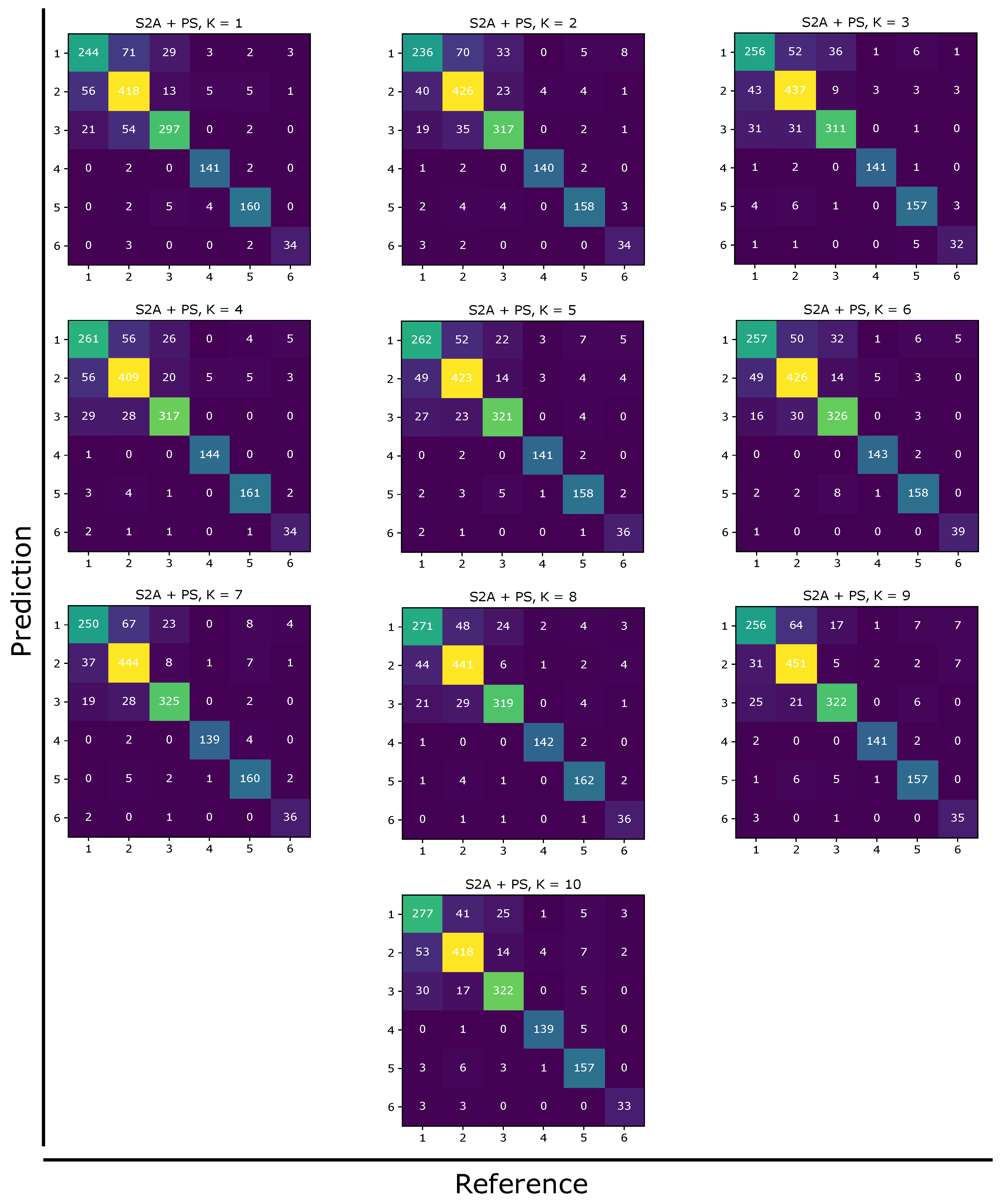
Beyond qualitative differences in land cover maps, classification accuracies were quantified using a stratified 10-fold cross-validation approach and compared to further ascertain the utility of the different datasets. Accuracy results from confusion matrices (see Appendix A.1) are presented in Figure 6 and Table 2 for the whole landscape and individual land cover types respectively. Overall, the higher spatial resolution images (Fused and Planet images at 4.77m spatial resolution) gave relatively consistent and precise estimates of general land cover classification accuracies compared to the 10 m resolution Sentinel-2A image, which had a wider interquatile range of cross-validation accuracy scores (Figure 6). Aggregate accuracy scores for the Fused image were marginally higher, achieving an average F-score of , compared to Planet and Sentinel-2A images with average F-score values of and respectively.
At the level of individual land cover types, classification accuracy scores obtained from the Fused image were higher than those from Sentinel-2A and Planet images for all land cover classes except woody cover (Table 2). Sentinel-2A produced more accurate classification of woody cover, in excess of over the Fused image and over the Planet image in terms of average F-score values. Grazing lawn classification accuracy followed a similar trend as the general map accuracy estimates, with the Fused image marginally outperforming Planet and Sentinel-2A images by (Table 2). All individual land cover classes were successfully discriminated at high accuracies across all datasets. The most obvious inter-class misclassifications occurred among the vegetation classes (see confusion matrices in Appendix A.1).
To determine the significance of accuracy differences among the three datasets, the Friedman chi-square () test for significant differences (at ) in F-scores for overall map and individual land cover types was used. The test results are presented in Table 3 with accompanying post-hoc analysis using Nemenyi test in Figure 7 for significantly different class accuracies. Only accuracy results from woody and bunch grass cover classifications showed significant differences in accuracy (Table 3).
For woody cover, the accuracy estimates from Fused and Planet image pairs were statistically similar, but each paired with results from Sentinel-2A showed significant differences (Figure 7). When comparing accuracy scores for bunch grass classification, results from the Planet image was significantly different from results derived from both Fused and Sentinel-2A images. However, comparing results from Fused and Sentinel-2A images showed no significant differences in bunch grass accuracy scores (Figure 7).
3.3. Feature Importance
Image feature importance estimates for each classification are presented in Figure 8. Generally, the original image bands contributed most to land cover classification accuracy, dominated by the blue, green and red image bands across all datasets. Additional features that comprised the five (5) most important features were near infrared and shortwave infrared-1 for Sentinel-2A, near infrared and Global Environmental Monitoring Index for Planet image and red edge-1 and shortwave infrared-1 for the Fused image (Figure 8). Textural features were in general the least important across all images.
4. Discussion
This study presents a multi-sensor pan-sharpening approach for utilizing the spectral properties of ESA’s Sentinel-2A data [2] and the high spatial resolution of the recently released Planet mosaics over the tropics [14], for enhanced land cover classification in a heterogeneous African savannah landscape. While the target spatial resolution of 4.77 m (from the Planet image) was achieved in the resulting Fused image (Figure 3) with high correlations between individual bands when compared with the Sentinel-2A data, land cover specific assessment revealed some spectral differences particularly in heterogeneous vegetation classes (see SSIM in Figure 4). Traditionally, images are subject to some degree of spectral distortion during pan-sharpening [60,61] which persist even when the panchromatic and multi-spectral bands used are from the same sensor. For example, Sarp [60] recorded a permanent loss of structural information in pan-sharpened Ikonos and Quickbird images. In the case of this study, the inherent distortion of spectral information from the pan-sharpening process could have been compounded by the use of different sensors with varying spectral response functions, though both Sentinel-2A and Planet images had been pre-processed to surface reflectance. Additionally, the slight differences in temporal window for image acquisition as well as the compositing methods used for data creation likely contributed to the observed spectral difference. For example, the Planet image is a six-month composite covering June 2019 through to December 2019 (i.e. dry season to early rainy season), and was derived using best available image pixel, whereas the Sentinel-2A image was derived as a median composite of all images between May 2019 and June 2019. Future data interoperability could be enhanced with the release of monthly composites of high resolution Planet imagery from September 2020 onward [14], promising more consistent spectral information with other multi-spectral sensors.
Despite the losses in structural information from pan-sharpening, the spectral integrity of the fused image was most evident in the relatively homogeneous and stable land cover types such as bare patches, built-up and water bodies, with relatively high SSIM statistics (Figure 4). This also translated into land cover classification in terms of spatial and thematic details (Figure 5) as well as accuracy outcomes (Figure 6 and Table 2). Having more spectral information covering the visible (3 bands), red edge (4 bands), near infrared (1 band) and shortwave infrared (2 bands) at a high spatial scale that can resolve most vegetation patches typical in a heterogeneous savannah landscape, enhanced land cover discrimination space leading to higher classification accuracies for the entire landscape. Another important finding to emerge from cross-validation accuracy analysis was the markedly low precision in Sentinel-2A accuracy scores, expressed in a much wider inter-quartile range compared to those from Planet and Fused images (Figure 6). In general, therefore, it seems that at coarse spatial scales, reference pixels used for training and validation are more prone to high intra-class variation, possibly emanating from the influence of adjacent land cover pixels due to lack of distinct boundaries. In the case of this study, this phenomenon was likely more pronounced due to the high heterogeneity within the studied savannah landscape. This finding suggests the need for extensive reference samples to guarantee consistently high accuracy scores when using Sentinel-2 or data with similar spatial characteristics in heterogeneous landscapes. It should be noted that the Fused image provided the most precise estimates of individual and overall land cover classification accuracies. Contrary to expectations, woody cover classification accuracy deviated from the pattern of dominance by the Fused image out of all individual land cover classes. The Sentinel-2A image achieved significantly higher woody cover classification accuracy, outperforming the Fused and Planet images by 4% and 6%, respectively, despite their higher spatial resolution. Depending on the size distribution of target land cover, medium resolution satellite images can produce similar or even better classification outcomes relative to high spatial resolution imagery [62].
Despite the visible loss of spatial detail in the coarser resolution Sentinel-2A image compared to the Planet and Fused images, all classifications produced very similar thematic representation of land cover (Figure 5). Marston et al [13] observed a similar phenomenon in a comparison of very high-resolution and medium resolution satellite image classifications. The marginal differences observed in classification accuracy among the three datasets (see class accuracies in Table 2) may be explained by results of feature importance estimates presented in Figure 8 which showed similarities in the most important contributing image features to classification accuracy. For example the first five (5) most important image features for classification were dominated by the visible bands (blue, green and red) across all datasets, which highlights the role of similar original image bands in all three classifications. The absence of additional red edge and shortwave infrared bands in the Planet image likely accounted for the differences in classification outcomes in comparison with the Fused image. The additional advantages of red edge bands for land cover mapping in vegetated landscapes have been widely reported in similar savannah applications [8,63,64,65]. For example, in a southern African savannah land cover classification context, Kaszta et al [8] found WorldView-2’s red edge band to be crucial in an object-based discrimination of vegetation components. The red edge band captures variations in vegetation pigmentation such as chlorophyll and carotenoids and thus enables successful discrimination of vegetation components even at the level of individual species [8,66]. Additionally, the shortwave infrared band is highly sensitive to vegetation moisture content due to higher levels of absorption and helps to highlight differences in vegetation states particularly in drier regions such as savannahs [67]. When comparing the Fused and Sentinel-2A classifications, similar feature importance estimates were observed for the first five (5) most important image features, with four (4) covering the blue, green, red and shortwave infrared bands. The only difference was the inclusion of near infrared for the Sentinel-2A image and red edge for the Fused image. It can therefore be assumed that the observed accuracy differences between these datasets occurred due to the influence of image spatial resolution. Spatial resolution is widely known to influence classification accuracy, with a general trend favouring higher spatial resolution [62,68,69]. Few studies however report on the accuracy effects of spatial resolution in heterogeneous savannah land cover classification. Our finding is consistent with Marston et al. [13] who recorded higher classification accuracies using VHR imagery than medium resolution images over the same southern African savannah landscape. Similarly, Allan [70] tested the influence of spatial resolution on savannah land cover classification by comparing SPOT-5, Landsat TM and MODIS sensors and recorded higher accuracy at finer spatial resolution. It is noteworthy that in both studies [13,70], the authors used imagery with different spectral properties unlike the similar spectral properties of Fused and Sentinel-2A used in this study. We suggest that optimization of savannah land cover classification would benefit from further robust experimentation of the combinations of spatial resolution and spectral properties that enhance accuracy. Overall, our comparison of classifications derived from the three datasets highlight the combined advantages of high spatial resolution and gain in spectral information from image fusion to enhance land cover classification outcomes.
This study demonstrates the potential of harnessing open-access satellite data for monitoring savannah land cover dynamics. Originally intended for deforestation monitoring over tropical regions, the Planet-NICFI images come as analysis ready cloud-free composites delivered as both biannual (every six months from December 2015 to August 2020) and monthly collections (from September 2020 onward) [14,71]. The free availability of such high resolution analysis ready data (ARD), in addition to the proliferation of cloud-based processing platforms, promises a rapid analysis of savannah vegetation attributes at landscape-scale to better understand patterns across different environmental gradients. Of particular interest are the impacts of contemporary threats to savannah ecosystem functioning such as widespread woody vegetation encroachment [72,73,74] and frequent, intense and long drought events [75,76], on the occurrence and distribution of grazing lawn communities, which are key food resources for mega-herbivores (such as rhinos) and important regulators of fire behaviour. A substantial extent of grazing lawn cover occurs at the footslopes of catenas adjacent to drainage channels where most woody cover is concentrated (Figure 5). However, the current rate of woody cover intensification within their range of existence [77], coupled with post-drought amelioration of fire [75] and dissociation of grazers from grazing lawns [78], suggest a high likelihood of grazing lawn colonization by adjacent woody vegetation. The combination of historical archives and future acquisitions from Sentinel-2A and high spatial resolution Planet images therefore presents enormous opportunities to investigate such phenomena and recommend spatially targeted management actions.
5. Conclusions
With the proliferation of different open-access remote sensing datasets comes the opportunity to combine their complementary features for enhanced characterisation of target land cover types, particularly in heterogeneous landscapes. This study presents a multi-sensor image fusion approach for creating images with similar characteristics as the popular high-valued commercial high-resolution satellite images using freely available Sentinel-2A and high resolution Planet images. The utility of the Fused image compared with the original Sentinel-2A and Planet images were tested in the context of enhancing land cover classification in a heterogeneous savannah landscape. The results show that, image fusion yielded the highest and most precise estimates of land cover classification accuracies in a heterogeneous mesic savannah landscape. The coarser spatial resolution Sentinel-2A image produced a wider range of classification accuracy estimates based on cross-validation analysis, and thus was the least precise. This suggests that, the use of Sentinel-2 images and image data with similar spatial characteristics in heterogeneous landscapes may require more reference samples to ensure consistently high classification accuracy outcomes. The results also show that, depending on factors such as available image quality and degree of multi-sensor image interoperability - mainly due to variation in temporal overlap - as it relates to project objectives, Sentinel-2A or Planet imagery may be individually used for savannah land cover analysis given the observed marginal differences in classification accuracy and similarities in thematic details. Future work incorporating structural information of different vegetation components such as that provided by Sentinel-1 could further enhance classification outcomes. This study provides pioneering evidence for the utility of the recent Planet-NICFI mosaics for land cover classification in a heterogeneous savannah landscape. Ultimately, our findings set a foundation for cost-effective and accurate high resolution analysis of savannah ecosystems in the phase of contemporary threats to ecosystem functioning such as woody encroachment and frequent drought events.
Author Contributions
Conceptualization, K.T.A. and P.A.; methodology, K.T.A ; field work, K.T.A., P.A., I.P. software, K.T.A; writing—original draft preparation, K.T.A; writing—review and editing, K.T.A., P.A., I.P., I.P.J.S.; supervision, P.A., I.P.
Funding
The Department of Geography and Geology, Edge Hill University, provided funding for this study. Field work was supported by the 2019 Geographical Club Award with grant reference GCA 42/19, offered by the Royal Geographical Society (RGS_IBG).
Acknowledgments
We are grateful to South Africa National Parks (SANParks) Scientific Services for providing a conducive environment for our field campaign. We thank Corli Wigley-Coetsee, Samantha Mabuza and Obert Mathebula for providing logistical and administrative support during our field stay in KNP. We are also immensely grateful to game guards Martin Sarela and Annoit Mashele. Thanks to former colleague, Daniel Knight for his immense help in field data collection.
Conflicts of Interest
The authors declare no conflict of interest.
Appendix A. Supplementary Data
Appendix A.1. Confusion Matrices
Figure A1.
Confusion matrices from 10-fold classification and accuracy assessment of the Sentinel-2A image. S2A = Sentinel-2A, K = Iteration. For the land cover classes considered, Woody = 1, Bunch grass = 2, Grazing lawns = 3, Water body =4, Bare = 5 and Built-up = 6.
Figure A1.
Confusion matrices from 10-fold classification and accuracy assessment of the Sentinel-2A image. S2A = Sentinel-2A, K = Iteration. For the land cover classes considered, Woody = 1, Bunch grass = 2, Grazing lawns = 3, Water body =4, Bare = 5 and Built-up = 6.

Figure A2.
Confusion matrices from 10-fold classification and accuracy assessment of the Planet image. PS = Planet, K = Iteration. For the land cover classes considered, Woody = 1, Bunch grass = 2, Grazing lawns = 3, Water body =4, Bare = 5 and Built-up = 6.
Figure A2.
Confusion matrices from 10-fold classification and accuracy assessment of the Planet image. PS = Planet, K = Iteration. For the land cover classes considered, Woody = 1, Bunch grass = 2, Grazing lawns = 3, Water body =4, Bare = 5 and Built-up = 6.

Figure A3.
Confusion matrices from 10-fold classification and accuracy assessment of the Fused image. S2A+PS = Fused image, K = Iteration. For the land cover classes considered, Woody = 1, Bunch grass = 2, Grazing lawns = 3, Water body =4, Bare = 5 and Built-up = 6.
Figure A3.
Confusion matrices from 10-fold classification and accuracy assessment of the Fused image. S2A+PS = Fused image, K = Iteration. For the land cover classes considered, Woody = 1, Bunch grass = 2, Grazing lawns = 3, Water body =4, Bare = 5 and Built-up = 6.
References
- Wulder, M.A.; Masek, J.G.; Cohen, W.B.; Loveland, T.R.; Woodcock, C.E. Opening the archive: How free data has enabled the science and monitoring promise of Landsat. Remote Sensing of Environment 2012, 122, 2–10. [Google Scholar] [CrossRef]
- Drusch, M.; Del Bello, U.; Carlier, S.; Colin, O.; Fernandez, V.; Gascon, F.; Hoersch, B.; Isola, C.; Laberinti, P.; Martimort, P.; others. Sentinel-2: ESA’s optical high-resolution mission for GMES operational services. Remote sensing of Environment 2012, 120, 25–36. [Google Scholar] [CrossRef]
- Bastin, J.F.; Berrahmouni, N.; Grainger, A.; Maniatis, D.; Mollicone, D.; Moore, R.; Patriarca, C.; Picard, N.; Sparrow, B.; Abraham, E.M.; others. The extent of forest in dryland biomes. Science 2017, 356, 635–638. [Google Scholar] [CrossRef]
- Griffith, D.M.; Lehmann, C.E.; Strömberg, C.A.; Parr, C.L.; Pennington, R.T.; Sankaran, M.; Ratnam, J.; Still, C.J.; Powell, R.L.; Hanan, N.P.; others. Comment on “The extent of forest in dryland biomes”. Science 2017, 358. [Google Scholar] [CrossRef] [PubMed]
- Liu, Y.; Hill, M.J.; Zhang, X.; Wang, Z.; Richardson, A.D.; Hufkens, K.; Filippa, G.; Baldocchi, D.D.; Ma, S.; Verfaillie, J.; others. Using data from Landsat, MODIS, VIIRS and PhenoCams to monitor the phenology of California oak/grass savanna and open grassland across spatial scales. Agricultural and Forest Meteorology 2017, 237, 311–325. [Google Scholar] [CrossRef]
- Symeonakis, E.; Higginbottom, T.P.; Petroulaki, K.; Rabe, A. Optimisation of savannah land cover characterisation with optical and SAR data. Remote Sensing 2018, 10, 499. [Google Scholar] [CrossRef]
- Borges, J.; Higginbottom, T.P.; Symeonakis, E.; Jones, M. Sentinel-1 and Sentinel-2 Data for Savannah Land Cover Mapping: Optimising the Combination of Sensors and Seasons. Remote Sensing 2020, 12, 3862. [Google Scholar] [CrossRef]
- Kaszta, Ż.; Van De Kerchove, R.; Ramoelo, A.; Cho, M.; Madonsela, S.; Mathieu, R.; Wolff, E. Seasonal separation of African savanna components using worldview-2 imagery: a comparison of pixel-and object-based approaches and selected classification algorithms. Remote Sensing 2016, 8, 763. [Google Scholar] [CrossRef]
- Awuah, K.T.; Aplin, P.; Marston, C.G.; Powell, I.; Smit, I.P. Probabilistic mapping and spatial pattern analysis of grazing lawns in Southern African savannahs using WorldView-3 imagery and machine learning techniques. Remote Sensing 2020, 12, 3357. [Google Scholar] [CrossRef]
- Bucini, G.; Saatchi, S.; Hanan, N.; Boone, R.B.; Smit, I. Woody cover and heterogeneity in the savannas of the Kruger National Park, South Africa. 2009 IEEE International Geoscience and Remote Sensing Symposium. IEEE, 2009, Vol. 4, pp. IV–334.
- Bucini, G.; Hanan, N.P.; Boone, R.B.; Smit, I.P.; Saatchi, S.S.; Lefsky, M.A.; Asner, G.P. Woody fractional cover in Kruger National Park, South Africa: remote sensing-based maps and ecological insights. In Ecosystem function in savannas: measurement and modeling at landscape to global scales; CRC Press, 2010; pp. 219–237.
- Cho, M.A.; Mathieu, R.; Asner, G.P.; Naidoo, L.; Van Aardt, J.; Ramoelo, A.; Debba, P.; Wessels, K.; Main, R.; Smit, I.P.; others. Mapping tree species composition in South African savannas using an integrated airborne spectral and LiDAR system. Remote Sensing of Environment 2012, 125, 214–226. [Google Scholar] [CrossRef]
- Marston, C.G.; Aplin, P.; Wilkinson, D.M.; Field, R.; O’Regan, H.J. Scrubbing up: multi-scale investigation of woody encroachment in a southern African savannah. Remote Sensing 2017, 9, 419. [Google Scholar] [CrossRef]
- Planet, T. Planet Application Program Interface: In Space for Life on Earth. San Francisco, CA. https://api.planet.com 2017.
- Francini, S.; McRoberts, R.E.; Giannetti, F.; Mencucci, M.; Marchetti, M.; Scarascia Mugnozza, G.; Chirici, G. Near-real time forest change detection using PlanetScope imagery. European Journal of Remote Sensing 2020, 53, 233–244. [Google Scholar] [CrossRef]
- Laso, F.J.; Benítez, F.L.; Rivas-Torres, G.; Sampedro, C.; Arce-Nazario, J. Land cover classification of complex agroecosystems in the non-protected highlands of the Galapagos Islands. Remote Sensing 2020, 12, 65. [Google Scholar] [CrossRef]
- Symeonakis, I.; Verón, S.; Baldi, G.; Banchero, S.; De Abelleyra, D.; Castellanos, G. Savannah land cover characterisation: a quality assessment using Sentinel 1/2, Landsat, PALSAR and PlanetScope 2019.
- Gao, Y.; Mas, J.F. A Comparison of the Performance of Pixel Based and Object Based Classifications over Images with Various Spatial Resolutions 2008.
- Van der Sande, C.; De Jong, S.; De Roo, A. A segmentation and classification approach of IKONOS-2 imagery for land cover mapping to assist flood risk and flood damage assessment. International Journal of applied earth observation and geoinformation 2003, 4, 217–229. [Google Scholar] [CrossRef]
- Blaschke, T.; Hay, G.J.; Kelly, M.; Lang, S.; Hofmann, P.; Addink, E.; Feitosa, R.Q.; Van der Meer, F.; Van der Werff, H.; Van Coillie, F.; others. Geographic object-based image analysis–towards a new paradigm. ISPRS journal of photogrammetry and remote sensing 2014, 87, 180–191. [Google Scholar] [CrossRef] [PubMed]
- Maxwell, A.E.; Warner, T.A. Differentiating mine-reclaimed grasslands from spectrally similar land cover using terrain variables and object-based machine learning classification. International Journal of Remote Sensing 2015, 36, 4384–4410. [Google Scholar] [CrossRef]
- Ali, I.; Cawkwell, F.; Dwyer, E.; Barrett, B.; Green, S. Satellite remote sensing of grasslands: from observation to management. Journal of Plant Ecology 2016, 9, 649–671. [Google Scholar] [CrossRef]
- Xu, D.; Chen, B.; Shen, B.; Wang, X.; Yan, Y.; Xu, L.; Xin, X. The classification of grassland types based on object-based image analysis with multisource data. Rangeland Ecology & Management 2019, 72, 318–326. [Google Scholar]
- Siddiqui, Y. The modified IHS method for fusing satellite imagery. ASPRS 2003 Annual Conference Proceedings. Anchorage, Alaska, 2003, pp. 5–9.
- Yocky, D.A. Image merging and data fusion by means of the discrete two-dimensional wavelet transform. JOSA A 1995, 12, 1834–1841. [Google Scholar] [CrossRef]
- Laben, C.A.; Brower, B.V. Process for enhancing the spatial resolution of multispectral imagery using pan-sharpening, 2000. US Patent 6,011,875.
- Jenerowicz, A.; Woroszkiewicz, M. The pan-sharpening of satellite and UAV imagery for agricultural applications. Remote Sensing for Agriculture, Ecosystems, and Hydrology XVIII. International Society for Optics and Photonics, 2016, Vol. 9998, p. 99981S.
- Rokni, K.; Ahmad, A.; Solaimani, K.; Hazini, S. A new approach for surface water change detection: Integration of pixel level image fusion and image classification techniques. International Journal of Applied Earth Observation and Geoinformation 2015, 34, 226–234. [Google Scholar] [CrossRef]
- Zhao, L.; Shi, Y.; Liu, B.; Hovis, C.; Duan, Y.; Shi, Z. Finer Classification of Crops by Fusing UAV Images and Sentinel-2A Data. Remote Sensing 2019, 11, 3012. [Google Scholar] [CrossRef]
- Venter, F.; Scholes, R.; Eckhardt, H. The abiotic template and its associated vegetation pattern In du Toit JT, Biggs HC, & Rogers KH (Eds.), The Kruger experience: Ecology and management of savanna heterogeneity (pp. 83–129), 2003.
- Hempson, G.P.; Archibald, S.; Bond, W.J.; Ellis, R.P.; Grant, C.C.; Kruger, F.J.; Kruger, L.M.; Moxley, C.; Owen-Smith, N.; Peel, M.J.; others. Ecology of grazing lawns in Africa. Biological Reviews 2015, 90, 979–994. [Google Scholar] [CrossRef]
- Venter, F.J. A classification of land for management planning in the Kruger National Park. PhD thesis, University of South Africa, 1991.
- Kleynhans, E.J.; Jolles, A.E.; Bos, M.R.; Olff, H. Resource partitioning along multiple niche dimensions in differently sized African savanna grazers. Oikos 2011, 120, 591–600. [Google Scholar] [CrossRef]
- Zizka, A.; Govender, N.; Higgins, S.I. How to tell a shrub from a tree: A life-history perspective from a S outh A frican savanna. Austral Ecology 2014, 39, 767–778. [Google Scholar] [CrossRef]
- Corcoran, J.; Knight, J.; Pelletier, K.; Rampi, L.; Wang, Y. The effects of point or polygon based training data on RandomForest classification accuracy of wetlands. Remote Sensing 2015, 7, 4002–4025. [Google Scholar] [CrossRef]
- Ma, L.; Li, M.; Ma, X.; Cheng, L.; Du, P.; Liu, Y. A review of supervised object-based land-cover image classification. ISPRS Journal of Photogrammetry and Remote Sensing 2017, 130, 277–293. [Google Scholar] [CrossRef]
- Sadeh, Y.; Zhu, X.; Dunkerley, D.; Walker, J.P.; Zhang, Y.; Rozenstein, O.; Manivasagam, V.; Chenu, K. Fusion of Sentinel-2 and PlanetScope time-series data into daily 3 m surface reflectance and wheat LAI monitoring. International Journal of Applied Earth Observation and Geoinformation 2021, 96, 102260. [Google Scholar] [CrossRef]
- Gorelick, N.; Hancher, M.; Dixon, M.; Ilyushchenko, S.; Thau, D.; Moore, R. Google Earth Engine: Planetary-scale geospatial analysis for everyone. Remote sensing of Environment 2017, 202, 18–27. [Google Scholar] [CrossRef]
- Louis, J.; Debaecker, V.; Pflug, B.; Main-Knorn, M.; Bieniarz, J.; Mueller-Wilm, U.; Cadau, E.; Gascon, F. Sentinel-2 sen2cor: L2a processor for users. Proceedings Living Planet Symposium 2016. Spacebooks Online, 2016, pp. 1–8.
- Wang, Z.; Bovik, A.C.; Sheikh, H.R.; Simoncelli, E.P. Image quality assessment: from error visibility to structural similarity. IEEE transactions on image processing 2004, 13, 600–612. [Google Scholar] [CrossRef]
- Avanaki, A.N. Exact global histogram specification optimized for structural similarity. Optical review 2009, 16, 613–621. [Google Scholar] [CrossRef]
- Vincent, O.R.; Folorunso, O.; others. A descriptive algorithm for sobel image edge detection. Proceedings of informing science & IT education conference (InSITE). Informing Science Institute California, 2009, Vol. 40, pp. 97–107.
- Roerdink, J.B.; Meijster, A. The watershed transform: Definitions, algorithms and parallelization strategies. Fundamenta informaticae 2000, 41, 187–228. [Google Scholar] [CrossRef]
- Jin, X. Segmentation-based image processing system, 2012. US Patent 8,260,048.
- Pinty, B.; Verstraete, M. GEMI: a non-linear index to monitor global vegetation from satellites. Vegetatio 1992, 101, 15–20. [Google Scholar] [CrossRef]
- Laosuwan, T.; Uttaruk, P. Estimating tree biomass via remote sensing, MSAVI 2, and fractional cover model. IETE Technical Review 2014, 31, 362–368. [Google Scholar] [CrossRef]
- Haralick, R.M.; Shanmugam, K.; Dinstein, I.H. Textural features for image classification. IEEE Transactions on systems, man, and cybernetics 1973, 610–621. [Google Scholar] [CrossRef]
- Pratt, W.K. Introduction to Digital Image Processing, 1st ed.; CRC Press: Boca Ranton, USA, 2013; p. 756. [Google Scholar]
- Goodfellow, I.; Bengio, Y.; Courville, A. Deep learning; MIT press: Cambridge, USA, 2016; Available online: http://www.deeplearningbook.org.
- Bischof, H.; Schneider, W.; Pinz, A.J. Multispectral classification of Landsat-images using neural networks. IEEE transactions on Geoscience and Remote Sensing 1992, 30, 482–490. [Google Scholar] [CrossRef]
- Venkatesh, Y.; Raja, S.K. On the classification of multispectral satellite images using the multilayer perceptron. Pattern Recognition 2003, 36, 2161–2175. [Google Scholar] [CrossRef]
- Srivastava, N.; Hinton, G.; Krizhevsky, A.; Sutskever, I.; Salakhutdinov, R. Dropout: a simple way to prevent neural networks from overfitting. The journal of machine learning research 2014, 15, 1929–1958. [Google Scholar]
- Kingma, D.P.; Ba, J. Adam: A method for stochastic optimization. arXiv preprint arXiv:1412.6980 2014. arXiv:1412.6980. [CrossRef]
- Congalton, R.G.; Green, K. Assessing the accuracy of remotely sensed data: principles and practices, 3rd ed.; CRC press: Boca Ranton, USA, 2019; p. 346. [Google Scholar]
- Friedman, M. The use of ranks to avoid the assumption of normality implicit in the analysis of variance. Journal of the american statistical association 1937, 32, 675–701. [Google Scholar] [CrossRef]
- Friedman, M. A comparison of alternative tests of significance for the problem of m rankings. The Annals of Mathematical Statistics 1940, 11, 86–92. [Google Scholar] [CrossRef]
- Demšar, J. Statistical comparisons of classifiers over multiple data sets. The Journal of Machine Learning Research 2006, 7, 1–30. [Google Scholar]
- Nemenyi, P.B. Distribution-free multiple comparisons.; Princeton University, 1963.
- Pedregosa, F.; Varoquaux, G.; Gramfort, A.; Michel, V.; Thirion, B.; Grisel, O.; Blondel, M.; Prettenhofer, P.; Weiss, R.; Dubourg, V.; others. Scikit-learn: Machine learning in Python. the Journal of machine Learning research 2011, 12, 2825–2830. [Google Scholar]
- Sarp, G. Spectral and spatial quality analysis of pan-sharpening algorithms: A case study in Istanbul. European Journal of Remote Sensing 2014, 47, 19–28. [Google Scholar] [CrossRef]
- Pushparaj, J.; Hegde, A.V. Evaluation of pan-sharpening methods for spatial and spectral quality. Applied Geomatics 2017, 9, 1–12. [Google Scholar] [CrossRef]
- Awuah, K.T.; Nölke, N.; Freudenberg, M.; Diwakara, B.; Tewari, V.; Kleinn, C. Spatial resolution and landscape structure along an urban-rural gradient: Do they relate to remote sensing classification accuracy?–A case study in the megacity of Bengaluru, India. Remote Sensing Applications: Society and Environment 2018, 12, 89–98. [Google Scholar] [CrossRef]
- Forkuor, G.; Dimobe, K.; Serme, I.; Tondoh, J.E. Landsat-8 vs. Sentinel-2: examining the added value of sentinel-2’s red-edge bands to land-use and land-cover mapping in Burkina Faso. GIScience & remote sensing 2018, 55, 331–354. [Google Scholar]
- Otunga, C.; Odindi, J.; Mutanga, O.; Adjorlolo, C. Evaluating the potential of the red edge channel for C3 (Festuca spp.) grass discrimination using Sentinel-2 and Rapid Eye satellite image data. Geocarto International 2019, 34, 1123–1143. [Google Scholar] [CrossRef]
- Ngadze, F.; Mpakairi, K.S.; Kavhu, B.; Ndaimani, H.; Maremba, M.S. Exploring the utility of Sentinel-2 MSI and Landsat 8 OLI in burned area mapping for a heterogenous savannah landscape. Plos one 2020, 15, e0232962. [Google Scholar] [CrossRef]
- Pu, R.; Landry, S. A comparative analysis of high spatial resolution IKONOS and WorldView-2 imagery for mapping urban tree species. Remote Sensing of Environment 2012, 124, 516–533. [Google Scholar] [CrossRef]
- Bueno, I.T.; McDermid, G.J.; Silveira, E.M.; Hird, J.N.; Domingos, B.I.; Acerbi Júnior, F.W. Spatial Agreement among Vegetation Disturbance Maps in Tropical Domains Using Landsat Time Series. Remote Sensing 2020, 12, 2948. [Google Scholar] [CrossRef]
- Momeni, R.; Aplin, P.; Boyd, D.S. Mapping complex urban land cover from spaceborne imagery: The influence of spatial resolution, spectral band set and classification approach. Remote Sensing 2016, 8, 88. [Google Scholar] [CrossRef]
- Suwanprasit, C.; Srichai, N. Impacts of spatial resolution on land cover classification. Proceedings of the Asia-Pacific Advanced Network 2012, 33, 39. [Google Scholar] [CrossRef]
- Allan, K. Landcover classification in a heterogenous savanna environment: investigating the performance of an artificial neural network and the effect of image resolution. PhD thesis, 2007.
- Pandey, P.; Kington, J.; Kanwar, A.; Curdoglo, M. Addendum to Planet Basemaps Product Specifications: NICFI Basemaps. Technical Report Revision: v02, Planet Labs, 2021.
- Mitchard, E.T.; Flintrop, C.M. Woody encroachment and forest degradation in sub-Saharan Africa’s woodlands and savannas 1982–2006. Philosophical Transactions of the Royal Society B: Biological Sciences 2013, 368, 20120406. [Google Scholar] [CrossRef]
- Stevens, N.; Lehmann, C.E.; Murphy, B.P.; Durigan, G. Savanna woody encroachment is widespread across three continents. Global change biology 2017, 23, 235–244. [Google Scholar] [CrossRef]
- Case, M.F.; Staver, A.C. Fire prevents woody encroachment only at higher-than-historical frequencies in a South African savanna. Journal of Applied Ecology 2017, 54, 955–962. [Google Scholar] [CrossRef]
- Sankaran, M. Droughts and the ecological future of tropical savanna vegetation. Journal of Ecology 2019, 107, 1531–1549. [Google Scholar] [CrossRef]
- Case, M.F.; Wigley, B.J.; Wigley-Coetsee, C.; Carla Staver, A. Could drought constrain woody encroachers in savannas? African Journal of Range & Forage Science 2020, 37, 19–29. [Google Scholar]
- Zhou, Y.; Tingley, M.W.; Case, M.F.; Coetsee, C.; Kiker, G.A.; Scholtz, R.; Venter, F.J.; Staver, A.C. Woody encroachment happens via intensification, not extensification, of species ranges in an African savanna. Ecological Applications 2021, e02437. [Google Scholar] [CrossRef] [PubMed]
- Donaldson, J.E.; Parr, C.L.; Mangena, E.; Archibald, S. Droughts decouple African savanna grazers from their preferred forage with consequences for grassland productivity. Ecosystems 2020, 23, 689–701. [Google Scholar] [CrossRef]
Figure 1.
Map of study area showing location of the Nkhulu field site in Kruger National Park (KNP), with enlarged view of the Planet image scene (False colour: R, NIR, G) from NICFI overlaid with the Nkhulu exclosure boundary (sourced from South African National Parks Scientific Services). Inset map shows the location of KNP within South Africa.
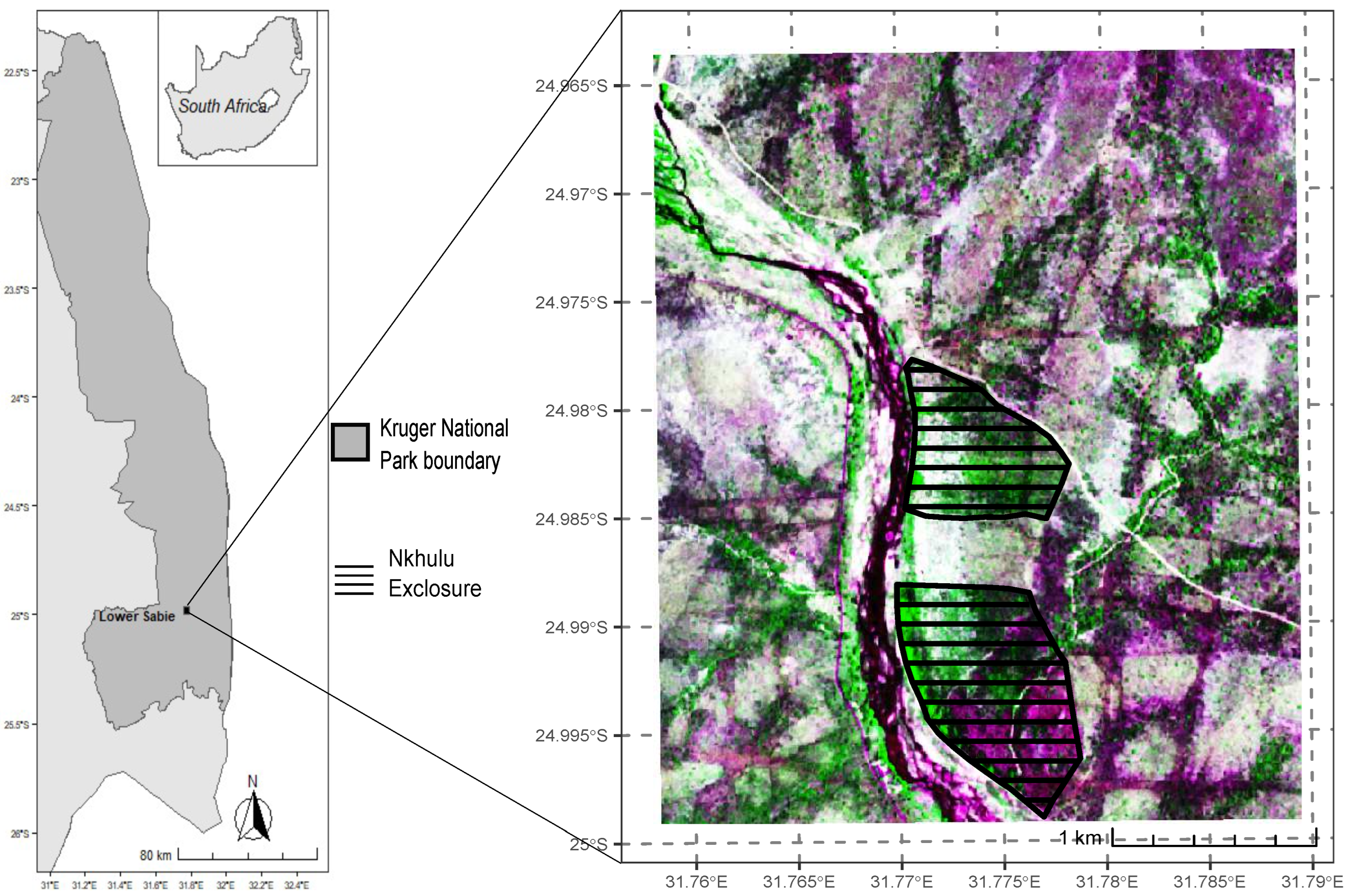
Figure 2.
Schematic representation of analysis workflow.
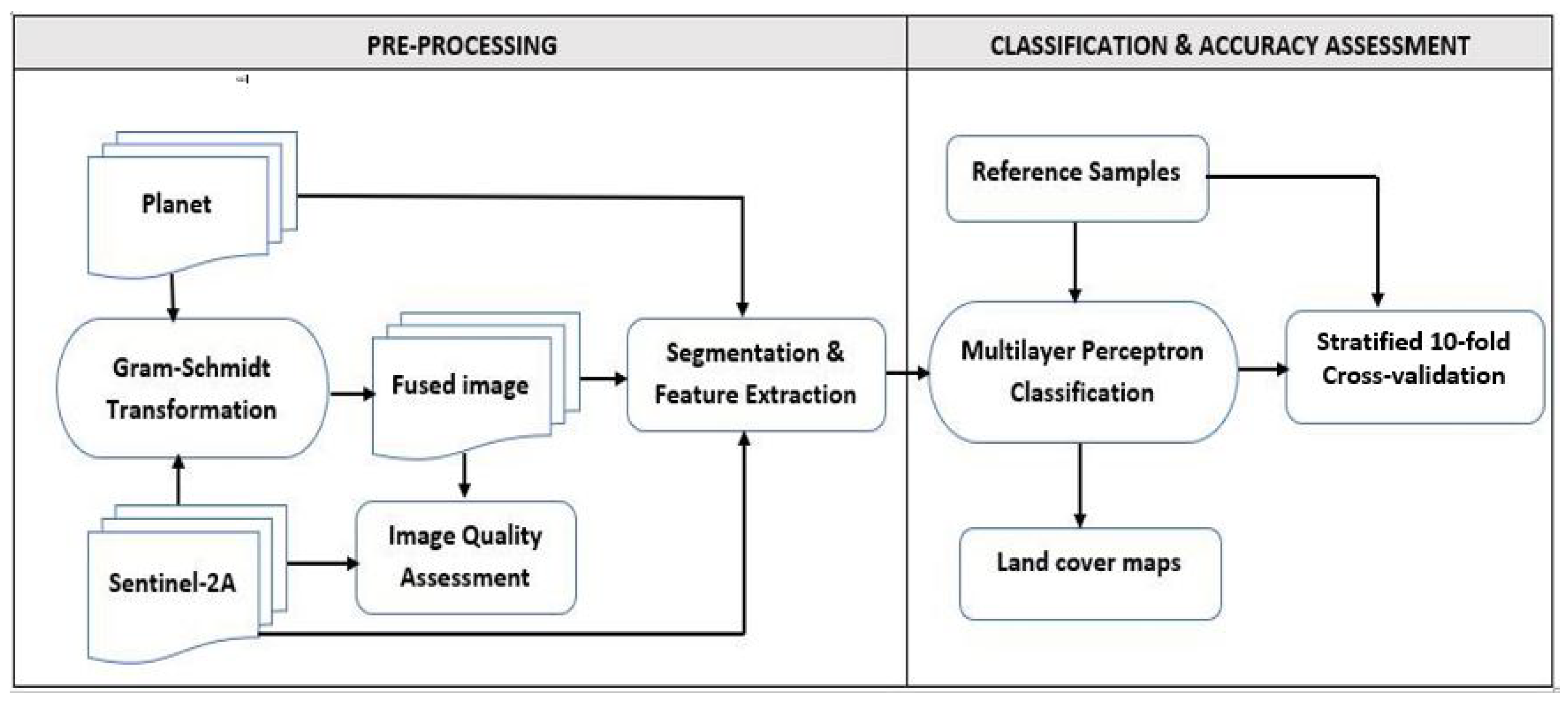
Figure 3.
False colour (R: NIR, G: Red, B: Green) display of original and fused images scenes of a sub-area. A visual comparison shows higher spatial resolution of Planet and Fused images relative to the Sentinel-2A image.
Figure 3.
False colour (R: NIR, G: Red, B: Green) display of original and fused images scenes of a sub-area. A visual comparison shows higher spatial resolution of Planet and Fused images relative to the Sentinel-2A image.
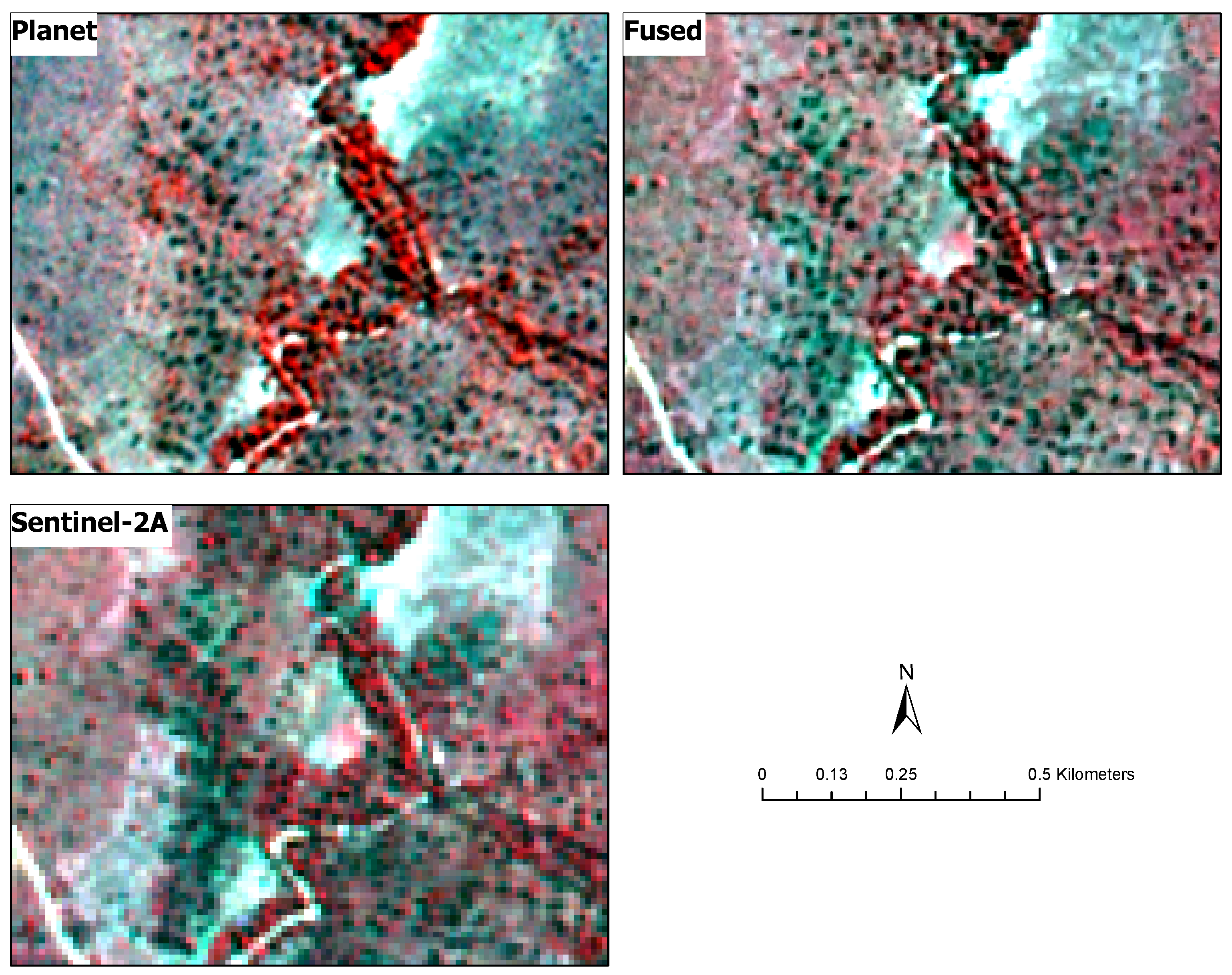
Figure 4.
Spectral quality metrics from pixel-level fusion. The figure shows Correlation Coefficient from Sentinel-2 and fused image band pairs (A) and boxplot showing summary of Structural Similarity Index (SSIM) for different savannah land cover types (B). B = Blue, G = Green, R = Red, RE-1 = Red Edge-1, RE-2 = Red Edge-2, RE-3 = Red Edge-3, NIR = Near Infrared, SWIR-1 = Short Wave Infrared-1 and SWIR-2 = Short Wave Infrared-2.
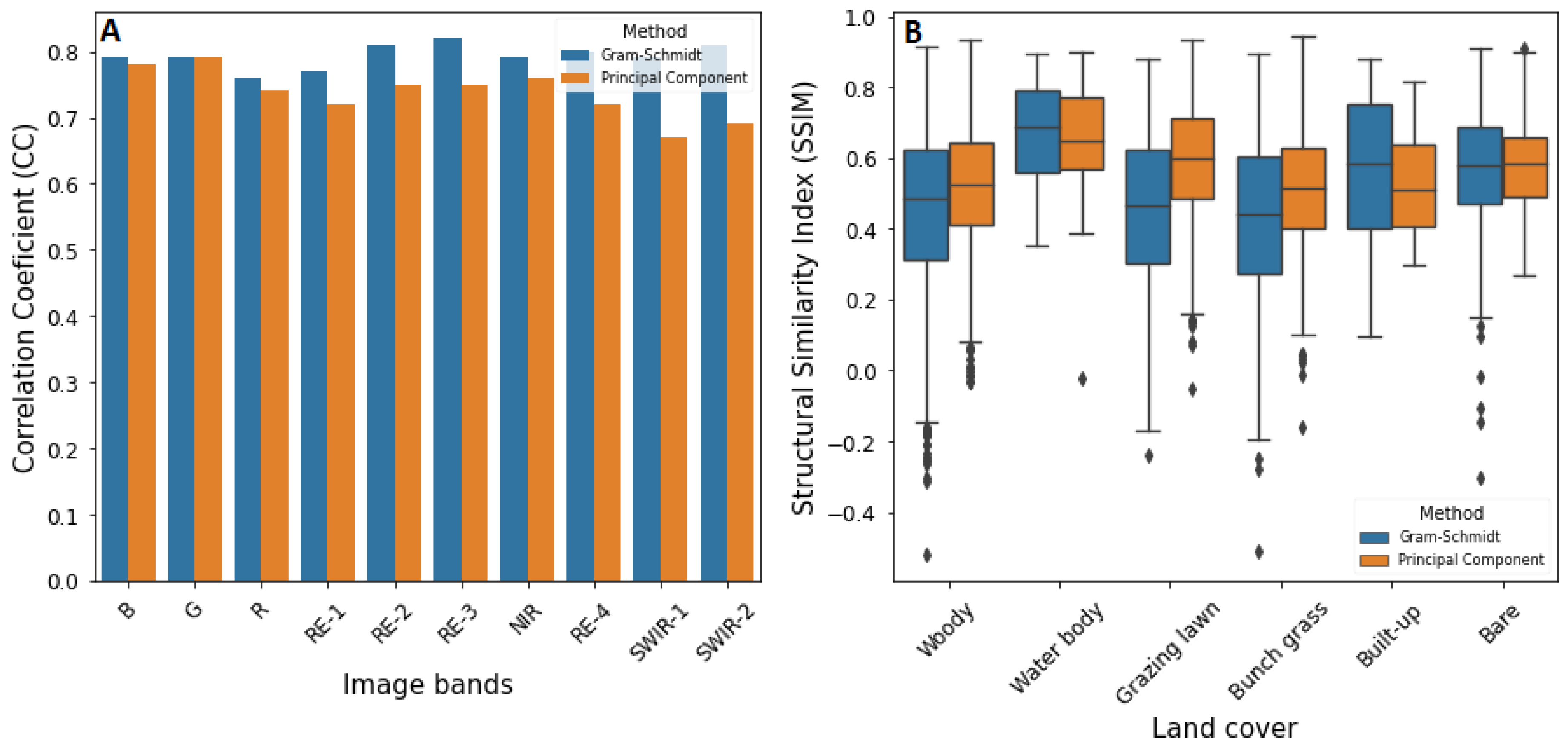
Figure 5.
Land cover maps derived from Planet (A), Fused (B) and Sentinel-2A (C) images.
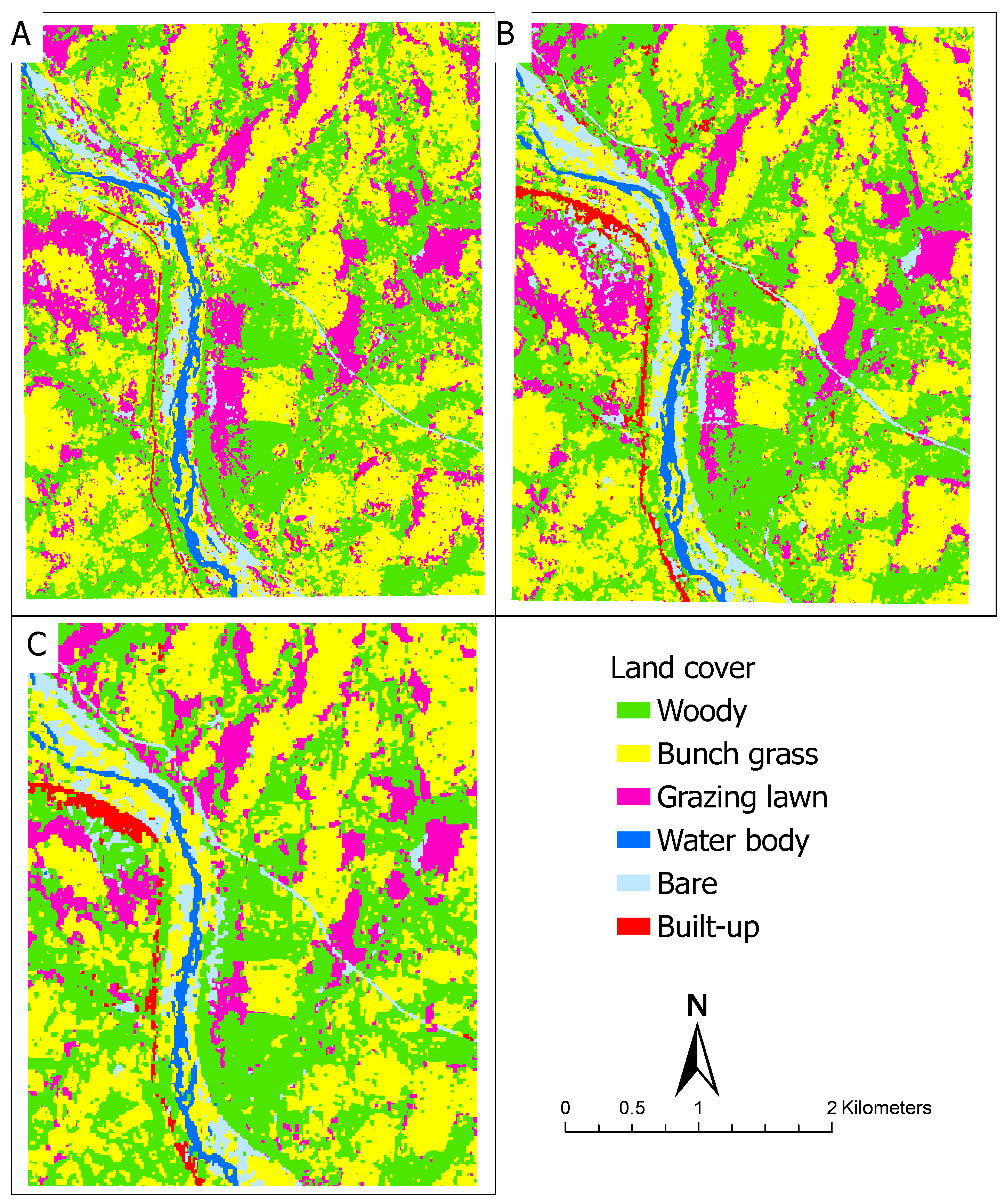
Figure 6.
General classification accuracies from stratified 10-fold cross-validation. Accuracy metrics were calculated as weighted averages from individual land cover class accuracies. Accuracy values represent fractions between 0 and 1.
Figure 6.
General classification accuracies from stratified 10-fold cross-validation. Accuracy metrics were calculated as weighted averages from individual land cover class accuracies. Accuracy values represent fractions between 0 and 1.
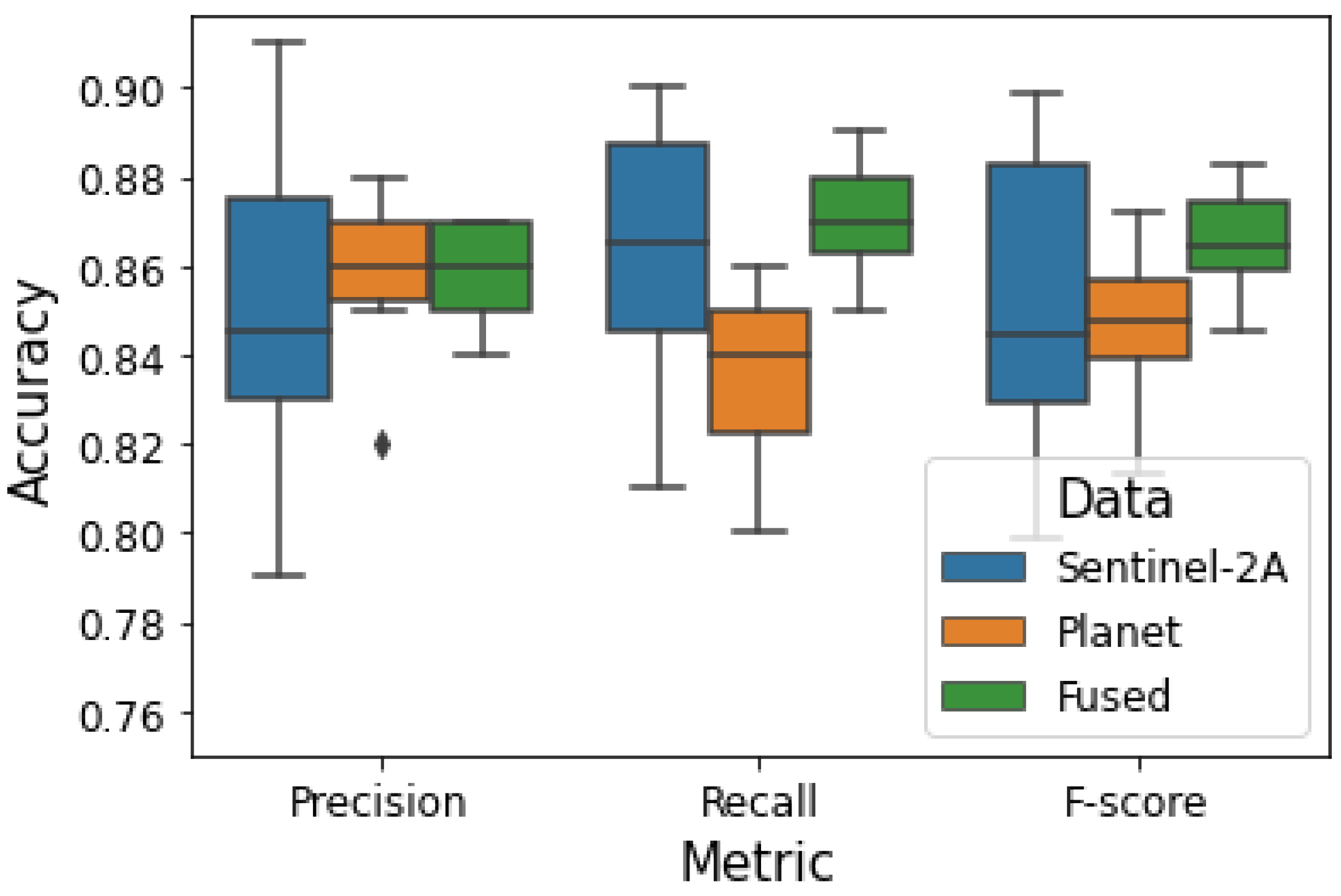
Figure 7.
Post-hoc comparison of Sentinel-2A, Planet and Fused datasets with Nemenyi test, based on F-scores for Woody and Bunch grass classes. Connected groups are not significantly different at . Critical Difference (CD) = 1.048
Figure 7.
Post-hoc comparison of Sentinel-2A, Planet and Fused datasets with Nemenyi test, based on F-scores for Woody and Bunch grass classes. Connected groups are not significantly different at . Critical Difference (CD) = 1.048
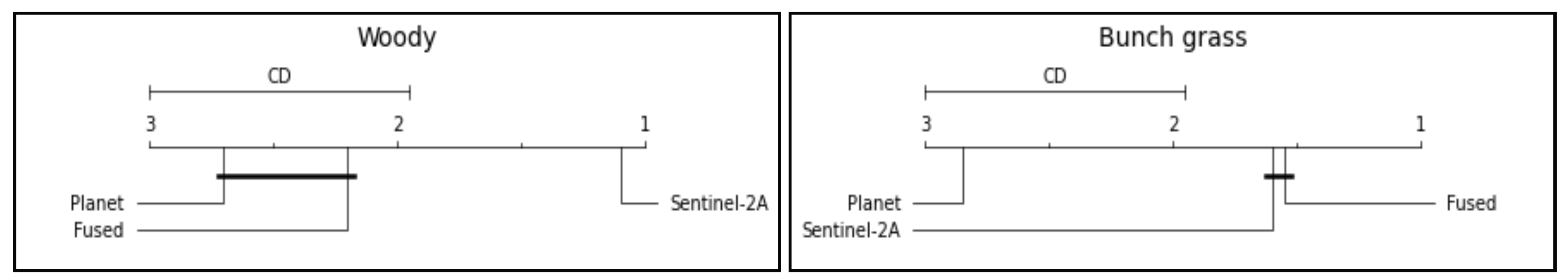
Figure 8.
Image feature importance estimates. Feature weights represent contribution to classification accuracy and is sorted in descending order. For feature acronyms, B = Blue, G = Green, R = Red, RE1 = Red Edge-1, RE2 = Red Edge-2, RE3 = Red Edge-3, RE4 = Red Edge-4, N = Near Infrared, SWIR1 = Shortwave Infrared-1, SWIR2 = Shortwave Infrared-2, GEMI = Global Environmental Monitoring Index, MSAVI2 = Modified Soil Adjusted Vegetation Index-2, Mean = Mean, Var = Variance, Savrg = Sum Average
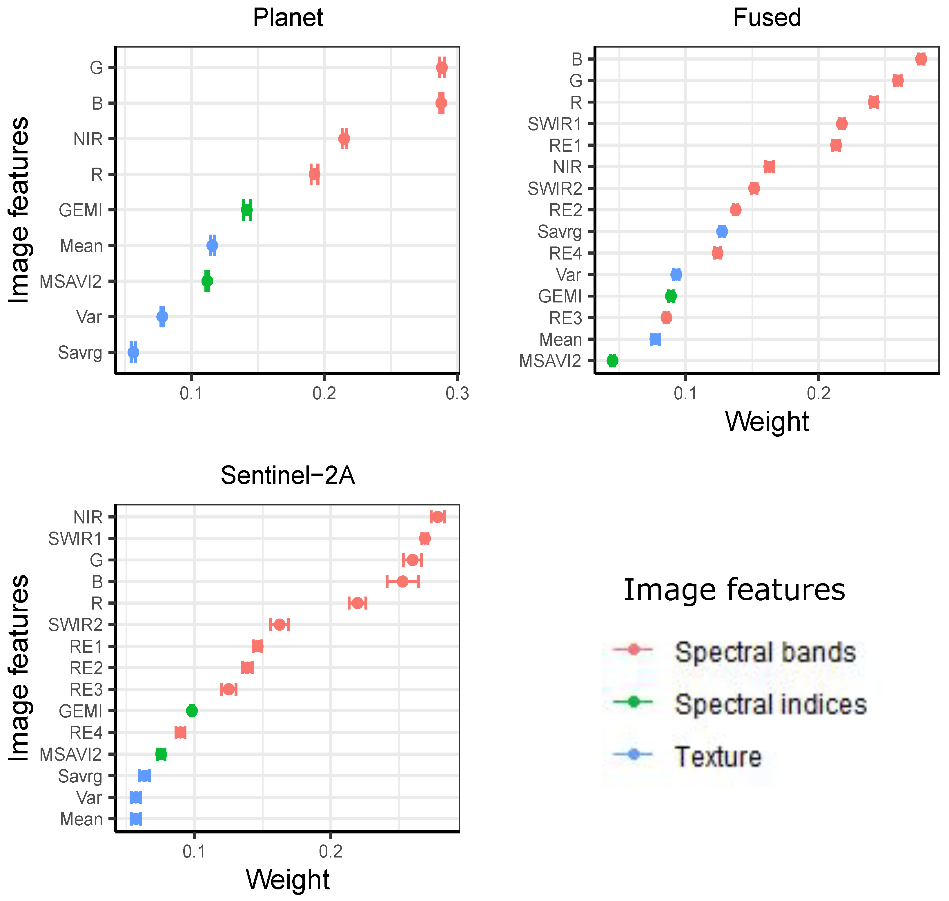

Table 1.
Description of land cover classification nomenclature and reference data. Reference samples are expressed as number of polygons and total area covered by polygons (in sq km) for each land cover class.
Table 1.
Description of land cover classification nomenclature and reference data. Reference samples are expressed as number of polygons and total area covered by polygons (in sq km) for each land cover class.
| Land cover | Reference samples | |||
|---|---|---|---|---|
| ID | Name | Description | Number of polygons | Area coverage () |
| 1 | Woody | Woody vegetation components including trees and shrubs at different phenological stages. |
1908 | 0.071 |
| 2 | Bunch grass | Tall grass patches often with upright growth form and dense distribution that are >20 cm in height. |
679 | 0.101 |
| 3 | Grazing lawn | Short grass patches with stoloniferous growth form and <20 cm in height, often sparsely distributed. |
457 | 0.077 |
| 4 | Water body | Water bodies occurring within the landscapes including rivers, streams and reservoirs. The landscape is mainly drained by the Sabie River. |
56 | 0.03 |
| 5 | Bare | Patches of exposed soil including dusty trails and rocky outcrops. | 262 | 0.034 |
| 6 | Built-up | Built artificial structures within the landscape, mostly asphalt and concrete coated surfaces such as roads and bridges and buildings. |
36 | 0.007 |
Table 2.
Summary of classification accuracy scores for savannah land cover types showing a comparison across dataset used (Sentinel-2A, Planet, Fused). Accuracy scores represent mean ± standard deviation from 10-fold stratified cross-validation. Accuracy values represent fractions between 0 and 1.
Table 2.
Summary of classification accuracy scores for savannah land cover types showing a comparison across dataset used (Sentinel-2A, Planet, Fused). Accuracy scores represent mean ± standard deviation from 10-fold stratified cross-validation. Accuracy values represent fractions between 0 and 1.
| Data | Land cover | Precision | Recall | F-score |
|---|---|---|---|---|
| Sentinel-2A | Woody | |||
| Bunch grass | ||||
| Grazing lawn | ||||
| Water body | ||||
| Bare | ||||
| Built-up | ||||
| Planet | Woody | |||
| Bunch grass | ||||
| Grazing lawn | ||||
| Water body | ||||
| Bare | ||||
| Built-up | ||||
| Fused | Woody | |||
| Bunch grass | ||||
| Grazing lawn | ||||
| Water body | ||||
| Bare | ||||
| Built-up |
Table 3.
Summary of Friedman chi-square () test for significant differences (at ) in accuracy scores for overall map and individual land cover types. Significance test was conducted on F-scores from stratified 10-fold cross-validation.
Table 3.
Summary of Friedman chi-square () test for significant differences (at ) in accuracy scores for overall map and individual land cover types. Significance test was conducted on F-scores from stratified 10-fold cross-validation.
| Land cover | Friedman statistic () | p-value |
|---|---|---|
| Woody | 14.11 | 0.00 |
| Bunch grass | 12.05 | 0.00 |
| Grazing lawn | 3.44 | 0.18 |
| Water body | 6.06 | 0.05 |
| Bare | 4.15 | 0.13 |
| Built-up | 2.00 | 0.37 |
| All | 5.60 | 0.06 |
Disclaimer/Publisher’s Note: The statements, opinions and data contained in all publications are solely those of the individual author(s) and contributor(s) and not of MDPI and/or the editor(s). MDPI and/or the editor(s) disclaim responsibility for any injury to people or property resulting from any ideas, methods, instructions or products referred to in the content. |
© 2024 by the authors. Licensee MDPI, Basel, Switzerland. This article is an open access article distributed under the terms and conditions of the Creative Commons Attribution (CC BY) license (http://creativecommons.org/licenses/by/4.0/).
Copyright: This open access article is published under a Creative Commons CC BY 4.0 license, which permit the free download, distribution, and reuse, provided that the author and preprint are cited in any reuse.


