The Cosmic Tapestry: A Comprehensive Study of Structure Formation

Richard Murdoch Montgomery

doi:10.20944/preprints202412.2637.v1

Submitted:

28 December 2024

Posted:

31 December 2024

You are already at the latest version

Abstract

Abstract Structure formation is a cornerstone of modern cosmology, linking the primordial fluctuations generated in the early universe to the intricate arrangement of galaxies, galaxy clusters, and cosmic voids observed today. In this article, we explore the theoretical underpinnings of structure formation within the CDM (Lambda Cold Dark Matter) paradigm and its alternatives, bridging fundamental physics and observational data. We review the historical development of the field, discuss the most important mathematical formalisms, and offer insights from both analytical treatments and state-of-the-art cosmological simulations. We then detail the methodologies used in deriving key equations, emphasize the observational techniques employed for validation, and present a critical discussion of the successes and lingering challenges in our quest to understand the universe's large-scale structure.Author: Richard Murdoch MontgomeryUniversidade de São PauloContact: montgomery@alumni.usp.br Abstract Structure formation is a cornerstone of modern cosmology, linking the primordial fluctuations generated in the early universe to the intricate arrangement of galaxies, galaxy clusters, and cosmic voids observed today. In this article, we explore the theoretical underpinnings of structure formation within the CDM (Lambda Cold Dark Matter) paradigm and its alternatives, bridging fundamental physics and observational data. We review the historical development of the field, discuss the most important mathematical formalisms, and offer insights from both analytical treatments and state-of-the-art cosmological simulations. We then detail the methodologies used in deriving key equations, emphasize the observational techniques employed for validation, and present a critical discussion of the successes and lingering challenges in our quest to understand the universe's large-scale structure.

Keywords:

structure formation

;

cosmology

;

cosmic perturbations

;

primordial fluctuations

;

galaxy clustering

Subject:

Physical Sciences - Astronomy and Astrophysics

Section 1. Introduction

The study of structure formation constitutes one of the central pillars of modern cosmology, aiming to explain how the universe evolved from a nearly homogeneous, hot, and dense state (as evidenced by the cosmic microwave background, CMB) into a complex web containing galaxies, clusters, filaments, and cosmic voids. Early efforts focused on understanding small linear perturbations in density that, over billions of years, gravitationally collapsed into the cosmic tapestry we observe through deep sky surveys such as the Sloan Digital Sky Survey (SDSS) and the Dark Energy Survey (DES). These observations have confirmed the

Λ C D M

model-a framework in which cold dark matter (CDM) drives structure formation while dark energy accelerates cosmic expansion-though various refinements and alternatives continue to be explored (Peebles 1980; Weinberg 2008).

Section 1.1. Historical Developments

Developments in structure formation theory stretch back several decades, with early seminal work by James Peebles demonstrating how primordial density fluctuations grow through gravitational instability in an expanding universe (Peebles 1980; Peebles 1993). This body of work laid the foundation for more precise theoretical frameworks incorporating general relativity, gaugeinvariant perturbation theory, and robust statistical analysis of large-scale structure (Mukhanov, Feldman, and Brandenberger 1992).

Although the current standard model (

Λ C D M

) provides a remarkably successful description of largescale structure (LSS), there remain open questions about the nature of dark matter, the properties of dark energy, and possible modifications to general relativity on cosmic scales (Riess et al. 1998;Perlmutter et al. 1999; Planck Collaboration 2018). Recent progress has also been driven by advances in numerical methods and high-performance computing, enabling large N -body simulations that can track the evolution of billions of collisionless dark matter particles. These simulations guide our interpretation of galaxy surveys and help us constrain cosmological parameters with increasing precision.In this article, we present a comprehensive review of structure formation. After describing the physical foundations, including primordial fluctuations, linear and nonlinear growth of perturbations, and virialization, we discuss standard tools used in the field-such as the matter power spectrum, correlation functions, halo models, and sophisticated simulation techniques. We then highlight observational efforts that provide constraints on structure formation, including galaxy surveys, weak lensing measurements, and Lyman-

α

forest observations.

Section 1.2. How and Where?

In the methodology section, we derive the main theoretical equations, step by step, focusing on gauge-invariant perturbation theory and the Newtonian approximation in an expanding background. Throughout the text, we include relevant mathematical derivations to elucidate how structure formation emerges naturally from Einstein's field equations, coupled to fluid conservation laws, under the assumption of cosmological principle. The discussion offers an extended critical analysis of the strengths and limitations of our understanding, tackling issues such as potential tensions in the data (e.g., the so-called

σ_{8}

tension, the

H_{0}

tension) and the uncertain nature of dark matter. We close with concluding remarks pointing toward future directions of research in structure formation before presenting the references used.

Section 2. Methodology

In approaching the theory of structure formation, it is instructive to demonstrate where the key equations arise. While a full treatment requires the use of general relativity and gauge-invariant perturbation theory, one can glean many essential results from the Newtonian approximation, valid for sub-horizon scales in the late universe. We begin with a brief derivation of the relevant equations.

Section 2.1. The Background Cosmology

The homogeneous and isotropic background of our universe is well-described by the Friedmann-Lemaître-Robertson-Walker (FLRW) metric:

d s^{2} = - c^{2} d t^{2} + a^{2} (t) [\frac{d r^{2}}{1 - k r^{2}} + r^{2} (d θ^{2} + {s i n}^{2} θ d ϕ^{2})]

(1)

where

a (t)

is the scale factor,

k \in {- 1,0, 1}

describes the spatial curvature, and

c

is the speed of light. The scale factor satisfies the first Friedmann equation (Weinberg 2008):

H^{2} (t) = {(\frac{\dot{a}}{a})}^{2} = \frac{8 π G}{3} ρ_{t o t} - \frac{k c^{2}}{a^{2}} + \frac{Λ c^{2}}{3}

(2)

where

ρ_{tot}

is the total energy density of the universe,

G

is the gravitational constant, and

Λ

is the cosmological constant. The expansion rate is given by the Hubble parameter

H (t) \equiv \dot{a} (t) / a (t)

(3).

Section 2.2. Perturbation Equations in the Newtonian Approximation

In an expanding universe, structure formation proceeds via the growth of small inhomogeneities. One usually defines a density contrast

δ (x, t)

by:

δ (x, t) \equiv \frac{ρ (x, t) - \overline{ρ} (t)}{\overline{ρ} (t)}

(4)

where

ρ (x, t)

is the local matter density, and

\overline{ρ} (t)

is the mean matter density of the universe. If

| δ | ≪ 1

, then the growth of

δ

can be understood by linearizing the fluid and Poisson equations in a Newtonian framework. The continuity, Euler, and Poisson equations for a non-relativistic fluid in the expanding background are:

Continuity equation:

$\frac{\partial δ}{\partial t} + \frac{1}{a} \nabla \cdot v = 0$

(5)
Euler's equation (neglecting pressure for cold dark matter):

$\frac{\partial v}{\partial t} + H v + \frac{1}{a} (v \cdot \nabla) v = - \frac{1}{a} \nabla ϕ$

(6)
Poisson's equation:

$\nabla^{2} ϕ = 4 π G a^{2} \overline{ρ} δ$

(7)

Here,

v

is the peculiar velocity field, and

ϕ

is the gravitational potential associated with density fluctuations on sub-horizon scales. By further assuming the linear regime (

| δ | ≪ 1

and

v ≪ c

), one can neglect the term

(v \cdot \nabla) v

. Taking a time derivative of the continuity equation and substituting into the Euler equation while employing Poisson's equation yields the well-known linear evolution equation for

δ

:

\ddot{δ} + 2 H \dot{δ} - 4 π G \overline{ρ} δ = 0

(8)

The general solution of equation (8) is a superposition of a growing mode

D_{+} (t)

and a decaying mode

D_{-} (t)

. The growing mode

D_{+} (t)

is typically the relevant solution for structure formation. In an Einstein-de Sitter universe (i.e., matter-dominated, flat,

Ω_{m} = 1

),

D_{+} (t) \propto a (t) \propto t^{2 / 3}

. For other cosmological backgrounds, one must solve equation (8) numerically (Heath 1977). The above derivations highlight how structure formation emerges naturally in a universe filled with matter (baryonic and dark) that is allowed to clump under gravity. Coupling these equations to an initial power spectrum of perturbations (e.g., from inflation) allows one to predict statistical measures such as the matter power spectrum,

P (k)

, and correlation functions that describe how matter is distributed on different scales.

Section 2.3. Derivation of Primordial Fluctuations

A crucial ingredient in the theory of structure formation is the spectrum of primordial fluctuations, usually denoted

Δ_{R}^{2} (k)

or

P_{R} (k)

, where

R

is the comoving curvature perturbation. In the context of inflationary cosmology, quantum vacuum fluctuations are stretched to cosmological scales, generating a nearly scale-invariant distribution of density perturbations (Guth and Pi 1982; Liddle and Lyth 2000). After inflation, these modes re-enter the horizon, shaping the seeds of large-scale structure. The simplest single-field slow-roll inflationary models predict:

P_{R} (k) \propto k^{n_{s} - 4}

(9)

where

n_{s} \approx 1

is the scalar spectral index. The amplitude of these perturbations is usually quoted at the CMB pivot scale

k_{*} \approx 0.05 {M p c}^{- 1}

. Observations by the Planck satellite find

n_{s} \approx 0.96 - 0.97

(Planck Collaboration 2018).

Once these primordial perturbations enter the horizon in a matter-dominated or radiation dominated epoch, they evolve according to the linear theory described earlier, ultimately shaping the matter power spectrum

P (k)

at late times:

P (k, z) = D_{+}^{2} (z) T^{2} (k) P_{prim} (k)

(10)

where

T (k)

is the transfer function that encodes how different scales evolve through horizon crossing, radiation-matter equality, and other relevant epochs, while

D_{+} (z)

describes how fluctuations grow with redshift

z

. The primordial power spectrum

P_{prim} (k)

is determined from inflationary theory and calibrated by CMB measurements.

Section 2.4. Numerical Simulations and N-Body Methods

Analytical linear theory accurately describes early-times or large spatial scales, but fails when density perturbations become nonlinear (

| δ | ≳ 1

). To understand these late-time dynamics, researchers rely on N -body simulations in which the universe is discretized into "particles" representing collisionsless dark matter. The classical Poisson equation for gravity is solved on a discrete mesh or via tree-based algorithms to evolve the positions and velocities of particles forward in cosmic time (Efstathiou et al. 1985; Springel et al. 2005).

Early landmark simulations, such as the Millennium Simulation (Springel et al. 2005), tracked the evolution of over

10^{9}

particles in cubes several hundred megaparsecs on a side. More recent simulations like Illustris (Vogelsberger et al. 2014) and IllustrisTNG (Nelson et al. 2019) include baryonic processes-such as gas cooling, star formation, and feedback from supernovae and active galactic nuclei-by solving fluid equations on adaptive meshes or smoothed-particle hydrodynamics (SPH) codes (Teyssier 2002; Wadsley et al. 2004).Such simulations yield predictions for the distribution of dark matter halos, galaxy clustering, and various higher-order statistics such as bispectra. They also provide theoretical "mock catalogs" used for analyzing large-scale structure surveys. While progress has been remarkable, remaining uncertainties in baryonic physics, numerical resolution, and alternative dark matter scenarios (e.g., warm dark matter, self-interacting dark matter) drive ongoing research. Nevertheless, N -body simulations form a crucial component of the structure formation toolkit.

Section 2.5. Observational Constraints

Our knowledge of structure formation relies critically on comparing theoretical predictions to observations. Galaxy surveys such as the Sloan Digital Sky Survey (York et al. 2000), 2dF Galaxy Redshift Survey (Colless et al. 2001), and more recent efforts by DES, HSC, KiDS, and Euclid measure the three-dimensional positions of millions of galaxies, from which we can infer the matter correlation function, power spectrum, and various clustering statistics. Weak gravitational lensing surveys map the distribution of matter by measuring coherent distortions in the shapes of distant galaxies. The Lyman-

α

forest in quasar spectra probes the matter distribution at high redshifts (Croft et al. 1998). Together, these probes place stringent limits on cosmological parameters, such as

Ω_{m}

Ω_{Λ}, σ_{8}

, and the sum of neutrino masses (Planck Collaboration 2018). The synergy between different observational windows consistently favors

Λ C D M

, but significant tensions and open questions remain.

Figure 1. Graph 1. Dimensionless Matter Power Spectrum and Graph 2. Real-Space Correlation Function.

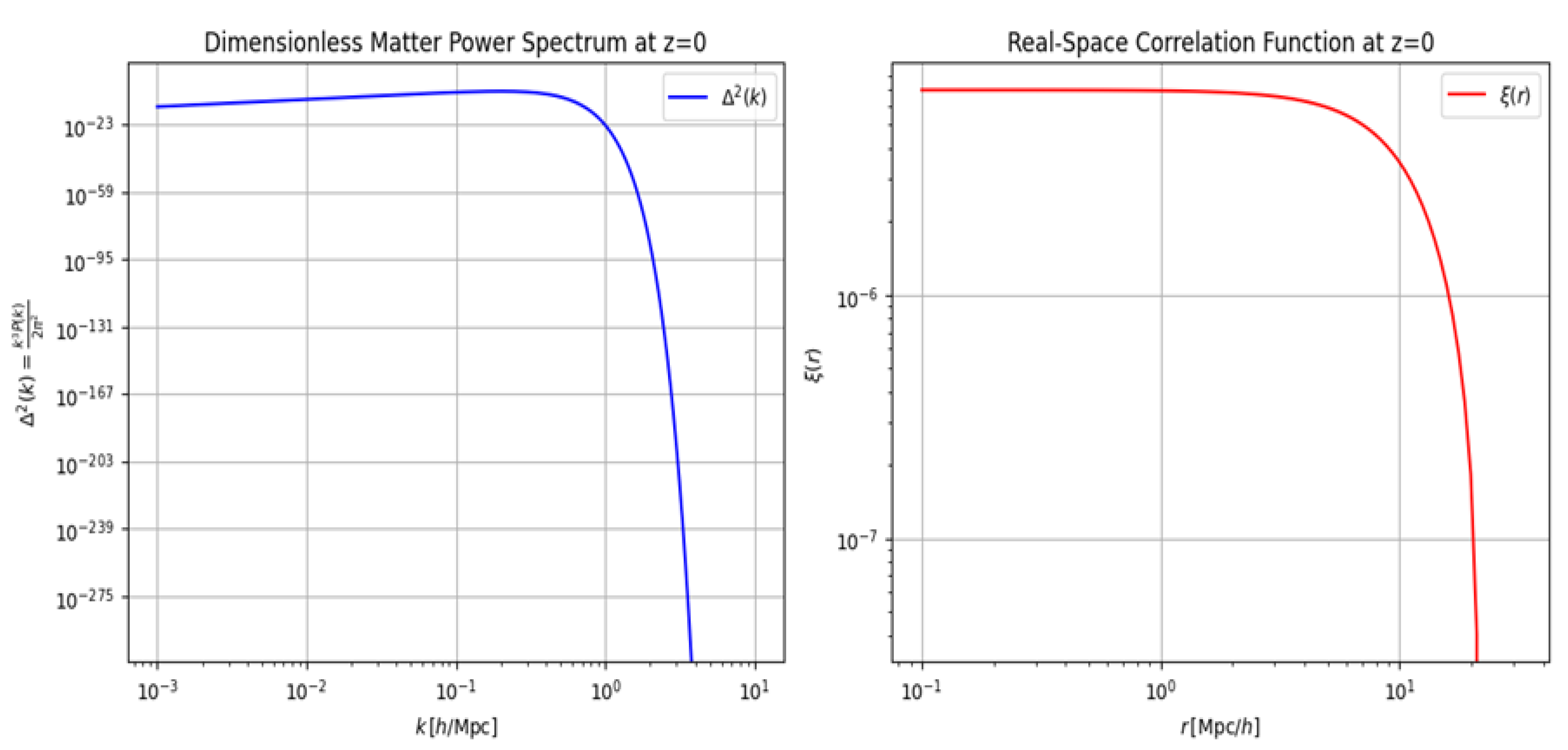
Section 2.6. Explanation of the Graphs

Graph 1. Dimensionless Matter Power Spectrum,

Δ^{2} (k)

:

The first graph displays the function

Δ^{2} (k) = \frac{k^{3}}{2 π^{2}} P (k)

which is often used to indicate the amount of variance (per logarithmic interval in

k

) contributed by modes of a given wavenumber. Where

Δ^{2} (k) \approx 1

, fluctuations at the corresponding scale are transitioning to the nonlinear regime. At

z = 0

in the standard

Λ

CDM scenario, nonlinear effects become important around

k \sim 0.1 h {M p c}^{- 1}

, although the exact scale depends on more rigorous calculations than our simple demonstration code.

Graph 2. Real-Space Correlation Function,

ξ (r)

:

The second graph shows the two-point correlation function in real space, defined by

ξ (r) = \frac{1}{2 π^{2}} \int_{0}^{\infty} d k k^{2} P (k) \frac{s i n (k r)}{k r}

This function measures the excess probability (relative to a random distribution) of finding matter pairs at a separation

r

. For instance, a positive

ξ (r)

at a certain scale means that matter is clustered above the random expectation at that distance, while negative

ξ (r)

would indicate an anti-correlation at that scale.

In more advanced analyses, one would use high-resolution Boltzmann codes to compute

P (k)

accurately across different epochs, include effects from baryons, neutrinos, and non-trivial dark energy models, and perform numerically stable integrals for

ξ (r)

. Nonetheless, these demonstrations illustrate two commonly plotted functions that help us interpret the clustering of matter in the universe.

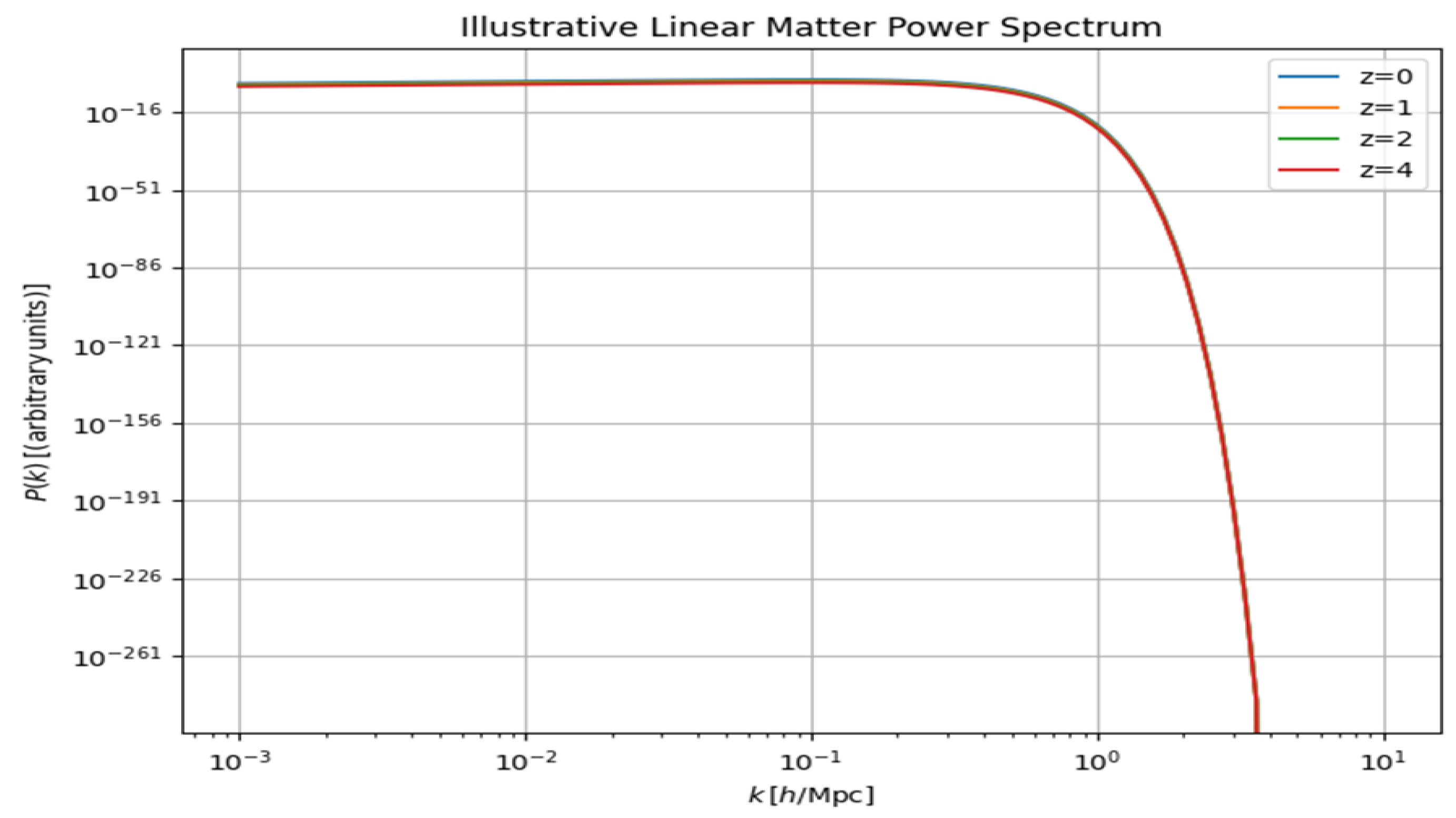
Figure 2. Graph 3. Illustrative Linear Matter Power Spectrum

This graph represents an illustrative linear matter power spectrum, showing the relationship between the wave number

k

(in units of

h / M p c

) and the power spectrum

P (k)

(in arbitrary units). The power spectrum

P (k)

is a key quantity in cosmology that describes how matter is distributed across different spatial scales in the universe.

Key Features:

Wave Number ( $k$ ):

$k$ is plotted on the x -axis and represents the inverse of spatial scale. Smaller values of $k$ correspond to large-scale structures, while larger values correspond to smaller-scale structures.

2.: Power Spectrum $(P (k))$ :

$P (k)$ is plotted on the $y$ -axis on a logarithmic scale. It quantifies the amount of clustering or fluctuation in matter at a given spatial scale.

3.: Redshift (z):

Different curves correspond to different redshift values $(z = 0,1, 2,4)$ . Redshift $z$ is a measure of how much the universe has expanded since the light from a structure was emitted. Higher $z$ indicates earlier times in the universe.

4.: Behavior of the Curves:

For small $k$ (large scales), $P (k)$ remains nearly constant. This indicates that fluctuations on large scales are relatively unchanging across different redshifts.
For larger $k$ (smaller scales), the power spectrum drops sharply. This drop corresponds to the suppression of small-scale fluctuations due to processes such as Silk damping or freestreaming.

5.: Impact of Redshift:

The curves for different redshifts $(z)$ are closely aligned, suggesting minimal evolution in the shape of the power spectrum over time in the linear regime.

Overall Interpretation:

The graph illustrates the general trend of the linear matter power spectrum across scales and its evolution over time (through redshift). On large scales (low

k

), structures are governed primarily by gravitational growth, while on small scales (high

k

), processes such as the pressure of baryonic matter or dark matter dynamics suppress the formation of structures.

Section 3. Discussion

The discussion on structure formation in cosmology is inherently rich and multifaceted, spanning an enormous range of scales, epochs, and physical processes. In this extended section, we delve into the merits (pros) of the standard picture and also highlight a variety of critiques and ongoing puzzles (cons). Although the standard

Λ C D M

model, complemented by the theory of inflation, has been remarkably successful, it is essential to critically examine its assumptions, domain of applicability, and potential extensions. By structuring this narrative within a fluid text, we aim to present a unifying perspective that does not shy away from the open challenges facing this field.A substantial point in favor of the standard scenario is its ability to account for an enormous range of observations with a surprisingly small set of parameters. When inflationary theory is invoked, the generation of near scale-invariant primordial fluctuations emerges organically from quantum physics under rapidly expanding space-time. These theoretical calculations accurately predict the СМВ angular power spectrum, which exhibits acoustic peaks consistent with baryon-photon oscillations in the early universe (Hu and Sugiyama 1995). The amplitude and shape of these peaks have been measured to exquisite precision by missions such as WMAP (WMAP Collaboration 2009) and Planck (Planck Collaboration 2018). In particular, the standard model makes a convincing link between early-universe physics and present-day structure formation by correctly forecasting the amplitude of matter fluctuations required to seed the formation of galaxies and clusters.One of the most striking accomplishments of this model lies in the robustness of the linear perturbation theory framework, which quantitatively predicts how cosmic overdensities grow during different epochs. Initially, these overdensities remain small, permitting a linear approximation. This approximation holds well until structures reach the scale of galaxy groups or clusters, at which point the nonlinear processes come into play. Even in the nonlinear regime, advanced numerical N -body simulations, performed with large supercomputers, verify that a universe dominated by cold dark matter can reproduce the large-scale distribution of galaxies and the cosmic web. The phenomenon known as "biased galaxy formation"-where galaxies trace underlying dark matter halos in a statistically biased manner-further cements the concordance picture when observed galaxy clustering is compared to dark matter distributions gleaned from simulations (Kaiser 1984; Bardeen et al. 1986).

Furthermore, the synergy of multiple observational probes has consistently reinforced the

Λ C D M

model. For instance, distant Type la supernovae measurements indicating cosmic acceleration, cosmic shear data from weak lensing surveys, and baryon acoustic oscillations (BAO) from galaxy surveys altogether fit within a single cosmological parameter space that strongly favors

Ω_{m} \approx 0.3

and

Ω_{Λ} \approx 0.7

. The high-redshift observations of the Lyman-

α

forest also show that small-scale fluctuations at redshifts around

2 - 3

align with

Λ C D M

predictions once the proper thermal history of the intergalactic medium is accounted for. This coherence across vastly different scales and epochs is one of the model's most substantial triumphs.Despite these successes, certain tensions and open questions stand out, revealing that cosmology is still a dynamic and evolving discipline. One of the most well-known tensions, often referred to as the Hubble tension, concerns the discrepancy between the Hubble constant

H_{0}

inferred from local distance ladder measurements (Riess et al. 2019) and that inferred from CMB data under the assumption of

Λ C D M

(Planck Collaboration 2018). While the latter method suggests

H_{0} \approx

67 k m s^{- 1} {M p c}^{- 1}

, local measurements yield values around

73 k m s^{- 1} {M p c}^{- 1}

. If this discrepancy persists with higher precision, it may indicate physics beyond the standard model, such as interactions within the dark sector, non-standard neutrino physics, or exotic forms of early dark energy.Another tension related to structure formation specifically concerns the amplitude of matter fluctuations, often quantified by

σ_{8}

, and the parameter

S_{8} = σ_{8} \sqrt{Ω_{m} / 0.3}

. Clustering measurements from weak lensing and redshift-space distortions sometimes yield slightly lower values of

σ_{8}

or

S_{8}

compared to those predicted by Planck data within

Λ

CDM (Joudaki et al. 2017; Heymans et al. 2021). This discrepancy, known as the

σ_{8}

or

S_{8}

tension, might be explained by systematic uncertainties in lensing measurements or incomplete modeling of baryonic feedback in simulations, but it might also point to interesting modifications in the growth of structure.Additionally, while cold dark matter is highly favored for explaining both cosmic microwave background power spectra and large-scale structure, it is not without its own challenges. On small galactic scales, longstanding issues such as the "core-cusp problem," the "missing satellites problem," and the "too-big-to-fail problem" linger (Bullock and Boylan-Kolchin 2017). These may be resolved by baryonic feedback mechanisms, or they may hint at alternative dark matter scenarios, such as self-interacting dark matter, warm dark matter, or fuzzy dark matter. Each scenario has distinct predictions for structure formation at small scales, particularly regarding subhalo abundance and internal halo density profiles.

Section 3.1. A further Realm of Theoretical Speculation

Science ca not still pro whether the law of gravity itself might require modification on large scales. Extensions to general relativity, commonly categorized under "modified gravity" theories, sometimes aim to explain cosmic acceleration without invoking a cosmological constant. These theories, however, must also consistently predict large-scale structure. Observables such as the growth rate of density perturbations, parameterized by

f σ_{8}

, the integrated Sachs-Wolfe effect, and gravitational lensing patterns, offer powerful constraints. While most modified gravity theories have been severely restricted by the data, the very existence of cosmic acceleration spurs ongoing exploration of gravity's behavior at large distances, even if

Λ C D M

remains the leading model.

Even if one accepts the standard gravitational framework, the precise nature of dark energy remains unexplored beyond the fact that it behaves almost exactly like a cosmological constant on cosmic scales. If the dark energy density does evolve over time, it could alter the growth of structure, especially at late times. Upcoming surveys such as the Vera C. Rubin Observatory's Legacy Survey of Space and Time (LSST), the Euclid mission, and the Nancy Grace Roman Space Telescope promise improved measurements of both expansion history and structure growth, potentially illuminating the dark energy sector.

Section 3.2. Methodological Breakthroughs

One should also acknowledge the methodological breakthroughs required to address some of these open questions, particularly regarding the interplay of astrophysical processes on smaller, nonlinear scales. Baryonic physics, including star formation, supernova feedback, and black hole accretion, can significantly affect the distribution of matter, especially at galaxy and cluster scales, by heating the surrounding gas and expelling it from halos, thus flattening the central density profiles. Accurately modeling these processes within large cosmological volumes demands advanced numerical techniques, sub-grid models, and more refined observational data to calibrate them. Discrepancies between different hydrodynamic codes-for instance, those employing smoothed-particle hydrodynamics versus adaptive mesh refinement-highlight the difficulties in robustly predicting baryonic effects on the matter power spectrum. In addition, phenomena such as cosmic reionization at high redshifts further complicate the modeling, linking large-scale structure with cosmic dawn and the formation of the first luminous objects.

Despite these many potential pitfalls, the general agreement of

Λ C D M

predictions with a wide range of data sets remains profoundly compelling. From the horizon-scale signatures in the CMB to the arrangement of galaxies and clusters in the local universe, the scenario of gravitational instability seeded by primordial quantum fluctuations consistently passes the test. Therefore, while caution dictates that we remain open to paradigmatic shifts if tensions worsen, the track record of successful predictions undeniably places

Λ C D M

at the forefront.

Moreover, the theoretical elegance of inflation as a mechanism for generating these primordial seeds cannot be overstated. It explains not only the amplitude and shape of the primordial power spectrum but also the overall flat geometry observed in the universe. Nonetheless, inflation is not a single theory but rather a framework that hosts a multitude of models, some of which predict distinctive secondary features (such as primordial non-Gaussianities, gravitational waves, or isocurvature modes). The continuing absence of a decisive detection of primordial B-mode polarization, for instance, imposes strong constraints on the energy scale of inflation. Equally, any future detection of a primordial gravitational wave background would be groundbreaking, shedding light on the scale at which inflation might have occurred.

Section 3.3. Summary

In summary, the "pros" of the standard picture are formidable: the generation of scale-invariant spectra from inflation, a matter-dominated regime that fosters gravitational instability, dark matter that clumps efficiently, and a late-time dark energy component that explains accelerated expansion. These yield coherent, parameter-light explanations for a deluge of observational data, from the CMB to the distribution of galaxies and clusters. The "cons" or challenges-manifesting as tensions in measured parameters, uncertainties in small-scale structure, theoretical ambiguities regarding inflation's specifics, the puzzling nature of dark energy-serve not to undermine the model's efficacy but to remind us that cosmology remains a vibrant field at the intersection of particle physics, astrophysics, and gravitational theory. The goal is not merely to confirm existing paradigms but to discover avenues where new physics may be lurking, waiting to reveal itself in subtle observational signatures or deeper theoretical insights. As experiments and surveys continue to push boundaries, we can expect the story of structure formation to become even richer, offering fresh perspectives on some of the most fundamental questions concerning our universe.

Altogether, the theory and observation of structure formation stands among the crowning achievements of contemporary science, weaving together advanced mathematics, high-performance computing, and extraordinary observational data into a tapestry that encapsulates cosmic history. While significant progress has been made, the field is far from complete, and the ongoing interactions of theory and observation will likely yield further revelations in the years to come.

Section 4. Conclusion

We have seen how structure formation has evolved into one of the most robust pillars of cosmology, connecting phenomena spanning the quantum fluctuations in the early universe to the distribution of galaxies in the late universe. Starting from a discussion of the FLRW metric and the associated Friedmann equations, we derived how small perturbations grow gravitationally to form the largescale structures we observe. We then highlighted the critical role of numerical simulations in going beyond linear theory, exploring how N -body codes allow us to track the nonlinear evolution of cosmic matter. Observational constraints, drawn from galaxy surveys, weak lensing, and the Lyman-

α

. forest, intersect with theoretical predictions, lending strong support to the

Λ

CDM model.

Nevertheless, open questions persist, including tensions in the measured values of the Hubble constant and the amplitude of matter fluctuations, uncertainties surrounding small-scale structure, and the nature of dark energy and dark matter. As we progress into an era of unprecedented observational precision, future surveys and missions will continue to refine our understanding and probe new windows in parameter space. The synergy of refined observations, sophisticated simulations, and theoretical innovation will undoubtedly reveal additional layers of complexity and may even unveil new physics beyond

Λ

CDM. In so doing, structure formation will continue to serve as a powerful lens through which we can seek answers to some of the most fundamental questions in cosmology.

Section 5. Attachments

Python Codes:

Graph 1 and 2:

import numpy as np

import matplotlib.pyplot as plt

# In this illustrative Python code, we will demonstrate the generation

# of a simplified linear matter power spectrum P(k) for different redshifts

# in a standard cosmology. This example is for didactic purposes and does

# not represent a rigorous calculation with a Boltzmann code such as CAMB

# or CLASS.

# We'll assume a simple transfer function and growth factor, ignoring

# baryonic effects, neutrinos, etc.

# Define array of wavenumbers in h/Mpc (log-spaced for convenience).

k_vals = np.logspace(-3, 1, 100)

# Define some cosmological parameters

Omega_m = 0.3

Omega_lambda = 0.7

h = 0.7

sigma8 = 0.8

n_s = 0.96

# Primordial power spectrum amplitude (arbitrary normalization in this example)

A_s = sigma8**2

# A simple approximation of the linear transfer function T(k) (not physically rigorous!)

def transfer_function(k):

# A naive approximation that saturates at small k and decays at large k

return np.exp(- (k/0.2)**2 )

# Define a simple growth factor for matter-dominated epoch (ignoring acceleration)

def growth_factor(z):

# Rough EdS behavior: D+(a) ~ a, with a = 1/(1+z)

# This is a crude approximation ignoring Lambda, for demonstration only.

a = 1.0 / (1.0 + z)

return a

# Let's compute the matter power spectrum P(k,z) ~ k^n_s * T(k)^2 * [D+(z)]^2

def matter_power_spectrum(k, z):

return A_s * k**n_s * transfer_function(k)**2 * growth_factor(z)**2

# For demonstration, we choose some redshifts

redshifts = [0, 1, 2, 4]

plt.figure(figsize=(8,6))

for z in redshifts:

pk = [matter_power_spectrum(kv, z) for kv in k_vals]

plt.loglog(k_vals, pk, label=f"z={z}")

plt.xlabel(r"$k \, [h/\mathrm{Mpc}]$")

plt.ylabel(r"$P(k) \, [\mathrm{(arbitrary\,units)}]$")

plt.title("Illustrative Linear Matter Power Spectrum")

plt.legend()

plt.grid(True)

plt.show()

The Python code above offers a simplified illustration of how one might compute and plot a linear matter power spectrum for different redshifts. In actual cosmological research, codes such as CAMB or CLASS solve a set of Boltzmann equations to compute a more accurate transfer function, taking into account the detailed physics of photons, neutrinos, baryons, and dark matter. Moreover, the growth factor in a ΛCDM universe deviates from the simple matter-dominated ∝a\propto a∝a dependence used here, thus requiring full integration of the linear perturbation equation (7) in the presence of a cosmological constant.

Overall, the code demonstrates how theoretical predictions of structure formation at various redshifts can be generated and visualized, representing a fundamental step before comparing these predictions to real data obtained from galaxy surveys or lensing measurements.

Graph 3.

import numpy as np

import matplotlib.pyplot as plt

from scipy.integrate import simps

# ========== Cosmological and Numerical Parameters ==========

Omega_m = 0.3

Omega_lambda = 0.7

h = 0.7

sigma8 = 0.8

n_s = 0.96

# A simple amplitude for the primordial spectrum (arbitrary normalization)

A_s = sigma8**2

# Define array of wavenumbers in h/Mpc (log-spaced for convenience).

k_vals = np.logspace(-3, 1, 200)

# ========== Simplified Transfer Function ==========

def transfer_function(k):

"""

A naive approximation of the transfer function that

saturates at low k and decays at high k. Not physically rigorous,

used for illustration only.

"""

return np.exp(-(k/0.2)**2)

# ========== Growth Factor (rough matter-dominated approximation) ==========

def growth_factor(z):

"""

For demonstration, we'll use the approximate EdS growth factor D+(a) ~ a,

ignoring Lambda for simplicity. In reality, one should solve the full

growth equation in a Lambda-CDM background.

"""

a = 1.0 / (1.0 + z)

return a

# ========== Matter Power Spectrum P(k,z) ==========

def matter_power_spectrum(k, z=0):

"""

Compute P(k,z) ~ A_s * k^n_s * T^2(k) * D+(z)^2

(with an arbitrary amplitude for demonstration).

"""

return A_s * k**n_s * transfer_function(k)**2 * growth_factor(z)**2

# ========== 1) Dimensionless Matter Power Spectrum, Delta^2(k) = k^3 * P(k) / 2pi^2 ==========

# We'll fix z = 0 for illustration.

z_plot = 0

pk_vals = matter_power_spectrum(k_vals, z=z_plot)

# Dimensionless power spectrum:

delta_sq_vals = (k_vals**3) * pk_vals / (2.0 * np.pi**2)

# ========== 2) Real-Space Correlation Function, xi(r) ==========

# The real-space correlation function is defined as:

# xi(r) = 1/(2*pi^2) * \int_0^\infty k^2 P(k) sin(k*r)/(k*r) dk

#

# We'll compute xi(r) at several distances r using a discrete integral.

def xi_of_r(r, k_array, pk_array):

"""

Compute the correlation function xi(r) = 1/(2*pi^2)

* integral[ k^2 * P(k) * sin(k*r)/(k*r) dk ],

using a simple numerical integration with sin(k*r)/(k*r).

"""

# Sinc function argument

kr = k_array * r

integrand = k_array**2 * pk_array * np.sin(kr) / kr

# Integrate using Simpson's rule over log-spaced k

return (1.0 / (2.0 * np.pi**2)) * simps(integrand, k_array)

# We'll define an array of radii (in Mpc/h) on which to compute xi(r).

r_vals = np.logspace(-1, 1.5, 100) # e.g., from 0.1 to ~ 31.6 Mpc/h

xi_vals = []

for r in r_vals:

xi_vals.append(xi_of_r(r, k_vals, pk_vals))

# ========== Plotting the Two Graphs ==========

plt.figure(figsize=(12, 5))

# --- Plot 1: Dimensionless Power Spectrum Delta^2(k) ---

plt.subplot(1, 2, 1)

plt.loglog(k_vals, delta_sq_vals, color='blue', label=r'$\Delta^2(k)$')

plt.xlabel(r'$k \, [h/\mathrm{Mpc}]$')

plt.ylabel(r'$\Delta^2(k) = \frac{k^3 P(k)}{2\pi^2}$')

plt.title('Dimensionless Matter Power Spectrum at z={}'.format(z_plot))

plt.grid(True)

plt.legend()

# --- Plot 2: Correlation Function xi(r) ---

plt.subplot(1, 2, 2)

plt.loglog(r_vals, xi_vals, color='red', label=r'$\xi(r)$')

plt.xlabel(r'$r \, [\mathrm{Mpc}/h]$')

plt.ylabel(r'$\xi(r)$')

plt.title('Real-Space Correlation Function at z={}'.format(z_plot))

plt.grid(True)

plt.legend()

plt.tight_layout()

plt.show()

Conflic of Interests

The Author claims there are no conflicts of interest.

References

Bardeen, J.M.; Bond, J.R.; Kaiser, N.; Szalay, A.S. The statistics of peaks of Gaussian random fields. The Astrophysical Journal 1986, 304, 15. [Google Scholar] [CrossRef]
Bullock, J.S.; Boylan-Kolchin, M. Small-scale challenges to the Λ\LambdaΛCDM paradigm. Annual Review of Astronomy and Astrophysics 2017, 55, 343–387. [Google Scholar] [CrossRef]
Colless, M.M.; Dalton, G.B.; Maddox, S.J.; Sutherland, W.J.; Norberg, P.; Cole, S.; et al. The 2dF Galaxy Redshift Survey: spectra and redshifts. Monthly Notices of the Royal Astronomical Society 2001, 328, 1039–1063. [Google Scholar] [CrossRef]
Croft, R.A.C.; Weinberg, D.H.; Katz, N.; Hernquist, L. Recovery of the power spectrum of mass fluctuations from observations of the Lyα\alphaα forest. The Astrophysical Journal 1998, 495, 44. [Google Scholar] [CrossRef]
Efstathiou, G.; Davis, M.; White, S.D.M.; Frenk, C.S. Numerical techniques for large cosmological N-body simulations. The Astrophysical Journal Supplement Series 1985, 57, 241. [Google Scholar] [CrossRef]
Guth, A.H.; Pi, S.Y. Fluctuations in the new inflationary universe. Physical Review Letters 1982, 49, 1110–1113. [Google Scholar] [CrossRef]
Heath, D.J. The growth of density perturbations in zero pressure Friedmann-Lemaître universes. Monthly Notices of the Royal Astronomical Society 1977, 179, 351–358. [Google Scholar] [CrossRef]
Heymans, C.; Tröster, T.; Asgari, M.; Blake, C.; Hildebrandt, H.; Joachimi, B.; et al. KiDS-1000 cosmology: Multi-probe weak gravitational lensing and spectroscopic galaxy clustering constraints. Astronomy Astrophysics 2021, 646, A140. [Google Scholar] [CrossRef]
Hu, W.; Sugiyama, N. Small-scale cosmological perturbations: An analytic approach. The Astrophysical Journal 1995, 444, 489–506. [Google Scholar] [CrossRef]
Joudaki, S.; Blake, C.; Heymans, C.; Choi, A.; Harnois-Deraps, J.; Hildebrandt, H.; et al. CFHTLenS revisited: assessing concordance with Planck including astrophysical systematics. Monthly Notices of the Royal Astronomical Society 2017, 465, 2033–2052. [Google Scholar] [CrossRef]
Kaiser, N. On the spatial correlations of Abell clusters. The Astrophysical Journal Letters 1984, 284, L9–L12. [Google Scholar] [CrossRef]
Liddle, A.R.; Lyth, D.H. (2000). Cosmological Inflation and Large-Scale Structure. Cambridge University Press.
Montgomery, R.M. (2024). Understanding the Hartman-Grobman Theorem: A Gateway to Predicting Dynamical System Behavior Near Hyperbolic Equilibria.Preprints,. [CrossRef]
Mukhanov, V.F.; Feldman, H.A.; Brandenberger, R.H. Theory of cosmological perturbations. Physics Reports 1992, 215, 203–333. [Google Scholar] [CrossRef]
Nelson, D.; Pillepich, A.; Springel, V.; Weinberger, R.; Genel, S.; Torrey, P.; et al. The IllustrisTNG simulations: public data release. Computational Astrophysics and Cosmology 2019, 6, 2. [Google Scholar] [CrossRef]
Peebles, P.J.E. (1980). The Large-Scale Structure of the Universe. Princeton University Press.
Peebles, P.J.E. (1993). Principles of Physical Cosmology. Princeton University Press.
Perlmutter, S.; Aldering, G.; Goldhaber, G.; Knop, R.A.; Nugent, P.; Castro, P.G.; et al. Measurements of Ω\OmegaΩ and Λ\LambdaΛ from 42 high-redshift supernovae. The Astrophysical Journal 1999, 517, 565–586. [Google Scholar] [CrossRef]
Planck Collaboration Planck 2018 results. VI. Cosmological parameters. Astronomy Astrophysics 2018, 641, A6. [Google Scholar]
Riess, A.G.; Filippenko, A.V.; Challis, P.; Clocchiatti, A.; Diercks, A.; Garnavich, P.M.; et al. Observational evidence from supernovae for an accelerating universe and a cosmological constant. The Astronomical Journal 1998, 116, 1009–1038. [Google Scholar] [CrossRef]
Riess, A.G.; Casertano, S.; Yuan, W.; Macri, L.M.; Scolnic, D. Large Magellanic Cloud Cepheid standards provide a 1% foundation for the determination of the Hubble constant and stronger evidence for physics beyond Λ\LambdaΛCDM. The Astrophysical Journal 2019, 876, 85. [Google Scholar] [CrossRef]
Springel, V.; White, S.D.M.; Jenkins, A.; Frenk, C.S.; Yoshida, N.; Gao, L.; et al. Simulations of the formation, evolution and clustering of galaxies and quasars. Nature 2005, 435, 629–636. [Google Scholar] [CrossRef]
Teyssier, R. Cosmological hydrodynamics with adaptive mesh refinement. Astronomy Astrophysics 2002, 385, 337–364. [Google Scholar] [CrossRef]
Vogelsberger, M.; Genel, S.; Springel, V.; Torrey, P.; Sijacki, D.; Xu, D.; et al. Introducing the Illustris project: simulating the coevolution of dark and visible matter in the Universe. Monthly Notices of the Royal Astronomical Society 2014, 444, 1518–1547. [Google Scholar] [CrossRef]
Wadsley, J.W.; Stadel, J.; Quinn, T. Gasoline: a flexible, parallel implementation of TreeSPH. New Astronomy 2004, 9, 137–158. [Google Scholar] [CrossRef]
Weinberg, S. (2008). Cosmology. Oxford University Press.
WMAP Collaboration Five-Year Wilkinson Microwave Anisotropy Probe Observations: Data Processing, Sky Maps, Basic Results. The Astrophysical Journal Supplement Series 2009, 180, 225–245. [CrossRef]
York, D.G.; Adelman, J.; Anderson, J.E.; Anderson, S.F.; Annis, J.; Bahcall, N.A.; et al. The Sloan Digital Sky Survey: Technical summary. The Astronomical Journal 2000, 120, 1579–1587. [Google Scholar] [CrossRef]

Figure 2. Graph 3. Illustrative Linear Matter Power Spectrum.

Disclaimer/Publisher’s Note: The statements, opinions and data contained in all publications are solely those of the individual author(s) and contributor(s) and not of MDPI and/or the editor(s). MDPI and/or the editor(s) disclaim responsibility for any injury to people or property resulting from any ideas, methods, instructions or products referred to in the content.

© 2024 by the authors. Licensee MDPI, Basel, Switzerland. This article is an open access article distributed under the terms and conditions of the Creative Commons Attribution (CC BY) license (http://creativecommons.org/licenses/by/4.0/).

Copyright: This open access article is published under a Creative Commons CC BY 4.0 license, which permit the free download, distribution, and reuse, provided that the author and preprint are cited in any reuse.

The Cosmic Tapestry: A Comprehensive Study of Structure Formation

Abstract

Keywords:

Subject:

Section 1. Introduction

Section 1.1. Historical Developments

Section 1.2. How and Where?

Section 2. Methodology

Section 2.1. The Background Cosmology

Section 2.2. Perturbation Equations in the Newtonian Approximation

Section 2.3. Derivation of Primordial Fluctuations

Section 2.4. Numerical Simulations and N-Body Methods

Section 2.5. Observational Constraints

Section 2.6. Explanation of the Graphs

Section 3. Discussion

Section 3.1. A further Realm of Theoretical Speculation

Section 3.2. Methodological Breakthroughs

Section 3.3. Summary

Section 4. Conclusion

Section 5. Attachments

Conflic of Interests

References

MDPI Initiatives

Important Links

Subscribe