
Submitted:
03 January 2025
Posted:
03 January 2025
You are already at the latest version
Abstract
Green asparagus has the characteristic of growing in clusters, making it inevitable for harvest targets to overlap with weeds and immature asparagus in the field. Extracting stem details in complex spatial positions information presents a significant challenge in identifying suitable harvest targets and high-precision cutting-points. This paper explored YS3AM (Yolo-SAM-3D-Adaptive-Modeling) method for green asparagus detection and 3D adaptive-section modeling using a depth camera, which could furnish harvesting path planning for the selective harvesting robots. Firstly, the model was developed and deployed to extract bounding boxes for individual asparagus stems within clusters. Secondly, the green asparagus stems within these bounding boxes were segment and generate binary mask images. Thirdly, high-quality depth images were obtained using pixel block completion. Finally, based on the cylinder, an adaptive-section 3D reconstruction method fusion with mask and depth was proposed, with a novel evaluation method applied to assess modeling accuracy. The experimental detection results of 1,095 test images demonstrated that the Precision was 98.75%, the Recall was 95.46%, the F1 score was 0.97, and the mAP was 97.16%. The modeling accuracy of 103 asparagus stems under sunny (54) and cloudy (49) conditions was estimated. The average RMSEs of length and bottom depth were 0.74 and 1.105. The detection and modeling for each stem approximately demanded 22 ms. The results of this paper indicated that the 3D model effectively represented the spatial distribution of green asparagus, and further accurately identification of suitable harvest targets and stem cutting-points. This model provided essential spatial pathways for end-effector path planning, thereby fulfilling the operational requirements for efficient green asparagus harvesting robot.
Keywords:
Green asparagus
; Clustered stem detection
; Selective harvesting
; Depth completion
; Adaptive 3D modeling
1. Introduction
Harvesting green asparagus is the most labor-intensive part of its production cycle (Clary et al., 2007) ,primarily relying on manual labor in China, which accounts for about 50% of production costs. Therefore, a harvesting robot capable of automatically harvesting green asparagus will significantly enhance productivity (Chen et al., 2021). However, accurate identification and segmentation and efficiency of green asparagus is difficult to meet the demands of operating equipment due to factors such as light fluctuations, plant overlap, camera angle, and distance, all of which have an impact on target detection in outdoor-grown green asparagus (Liu et al., 2022). Estimating spatial positions and key-points of harvesting objects also represents a crucial technical challenge in computer vision and provides important information for robotic harvesting. Therefore, for non-destructive and accurate green asparagus harvesting robots, in-field determination of accurately identifying clusters green asparagus and constructing a 3D growth model of green asparagus in unstructured environments is an important task.
Various imaging systems and AI-based image processing techniques offer a potential solution for accurately, robustly, and reliably monitoring of green asparagus growth and automated asparagus harvesting(Bac et al., 2014; Bargoti and Underwood, 2016; Dorj et al., 2017; Kondo and Ting, 1998). Irie et al. (Irie et al., 2009) proposed a harvesting robot that measured green asparagus cross-section and identified the target asparagus using a 3D vision sensor. Outdoor fruit and vegetable image recognition and localization are greatly affected by sunlight intensity and color temperature. One Japanese study (Sakai et al., 2013) employed dual laser sensors for the recognition and positioning of asparagus stem. This machine could avoid light for all-day work to meet the production demand.
With the development of Convolutional Neural Networks (CNNs), deep learning technology are promising for the detection of outdoor clustered green asparagus (Zheng et al., 2019). M. Peebles et al. (Peebles et al., 2019) employed Faster R-CNN (F-RCNN) (Ren et al., 2017) to detect green asparagus features in outdoor RGB images, and research the optimal network architecture for asparagus detection. Li (Li et al., 2021) proposed a recognition method combining image preprocessing with LeNet (Lecun et al., 1998) network during autonomous harvesting of green asparagus under outdoor natural lighting conditions. Hong (Hong et al., 2023; Wang et al., 2023) proposed an improved YOLO v5 algorithm that focuses more on the growth characteristics of asparagus, as well as the propagation and reusability of features.
The target detection algorithms mentioned performed well in simple backgrounds, focusing mainly on identifying asparagus. However, outdoor green asparagus typically grows in irregular clusters of 3-6 stems, often overlapping with obstacles like steel rods, mother asparagus and immature asparagus, which complicates detection and reduces harvesting efficiency (Li et al., 2022). In recent years, depth image-based cluster fruit and vegetable recognition (Xiang et al., 2013) has been used to improve cluster-growing fruit and vegetable detection systems in complex backgrounds. This technique utilized depth information based on the 2D shape of the cluster region to achieve recognition of each fruit and vegetable object in the cluster region. The method could have good recognition performance in the presence of mild occlusion of fruits and vegetables, but there were fewer studies related to green asparagus in clusters. Leu (Leu et al., 2017) developed a harvesting robot using an RGB-D vision sensor to capture the 3D positions of green asparagus, effectively using depth data regardless of color variations. Kennedy (Kennedy et al., 2019) introduced a ground-plane projection method combining multiple monocular cameras for better performance in green asparagus harvesting. WANG (Wang et al., 2023) improved YOLACT++ to establish spatial vectors for asparagus masks, determining cutting points at the base of mature asparagus. Mu(Mu et al., 2024) proposed the S2CPL model, utilizing RGB-D sensors for evaluating the suitability of selective harvesting and precise positioning of subsoil cutting point. While these studies had shown promising results in predicting harvesting points, they may exhibit reduced precision in point localization when compared to visualization models that integrate the complete asparagus stem structure. This potential limitation could adversely affect the integrity of planning harvesting pathways for green asparagus. The development of 3D models could significantly enhance the planning of harvesting paths for picking robots and aid in constructing stable fruit-picking robots (Chen et al., 2021; Hu et al., 2024). However, there was currently no research focused on the 3D modeling of green asparagus.
Extracting complex spatial positions information of clustered green asparagus stems presents a significant challenge in identifying suitable harvest targets and high-precision cutting-points. A novel combined detection network and 3D Reconstruction named YS3AM (Yolo-SAM-3D-Adaptive-Modeling) is proposed to address these challenges by detecting clustered green asparagus and constructing detailed 3D visual models in unstructured environments. The main contributions of this paper are as follows:
- (1)
- The YS3AM uses the improved YOLOv7 to detect individual asparagus stems within clusters, followed by the SAM algorithm to accurately segment each stem within prediction boxes.
- (2)
- The YS3AM model addresses incomplete depth data from the RGB-D sensor by filling in missing pixels using advanced interpolation techniques to preserve 3D model accuracy.
- (3)
- The YS3AM model merges stem masks with depth images to create an adaptive-section 3D model, enabling effective path planning of harvesting in unstructured environments.
2. Materials and Methods
2.1. Overview
The YS3AM model was composed of five principal components: acquiring RGB-D images of clustered green asparagus through a RGB-D sensor (Figure 1a), conducting detection on the augmented RGB images and achieving semantic segmentation (Figure 1b), completing the missing pixel blocks in the Depth images based on the Mask images, extracting the contours of green asparagus stems, and realizing the coordinate transformation of some key points from the pixel coordinate system to the camera coordinate system (Figure 1c), fitting the stalk curves based on the concept of equal segmentation, considering each stalk segment as a cylinder, and then calculating the length, center, and radius of each segment, combining the approximate cylinders of each asparagus segment into a 3D model (Figure 1d), and proposing the RMSE index to evaluate the overall accuracy of the model by computing the offsets of a few key-points, as well as presenting an adaptive-section modeling method based on the length of the asparagus stems, and finally establishing a high-precision spatial section model of green asparagus (Figure 1e).
2.2. Experimental Data
At present, there are many large-scale asparagus plantations throughout the country. After conducting field surveys, we found that green asparagus were planted in the soil ridge with a height of 15-20 cm, planting row spacing of 1.2-1.8 meters, plant spacing of 20-25 cm, and the diameter of each stem was 1.5-2 cm. The growth rate during the peak growth period is about 20 cm/d and the growth is relatively dense. This high density of stem conditions presents additional challenges for the machine vision systems, as harvesting targets are heavily obscured by weeds, or immature asparagus.
2.2.1. Data Acquisition
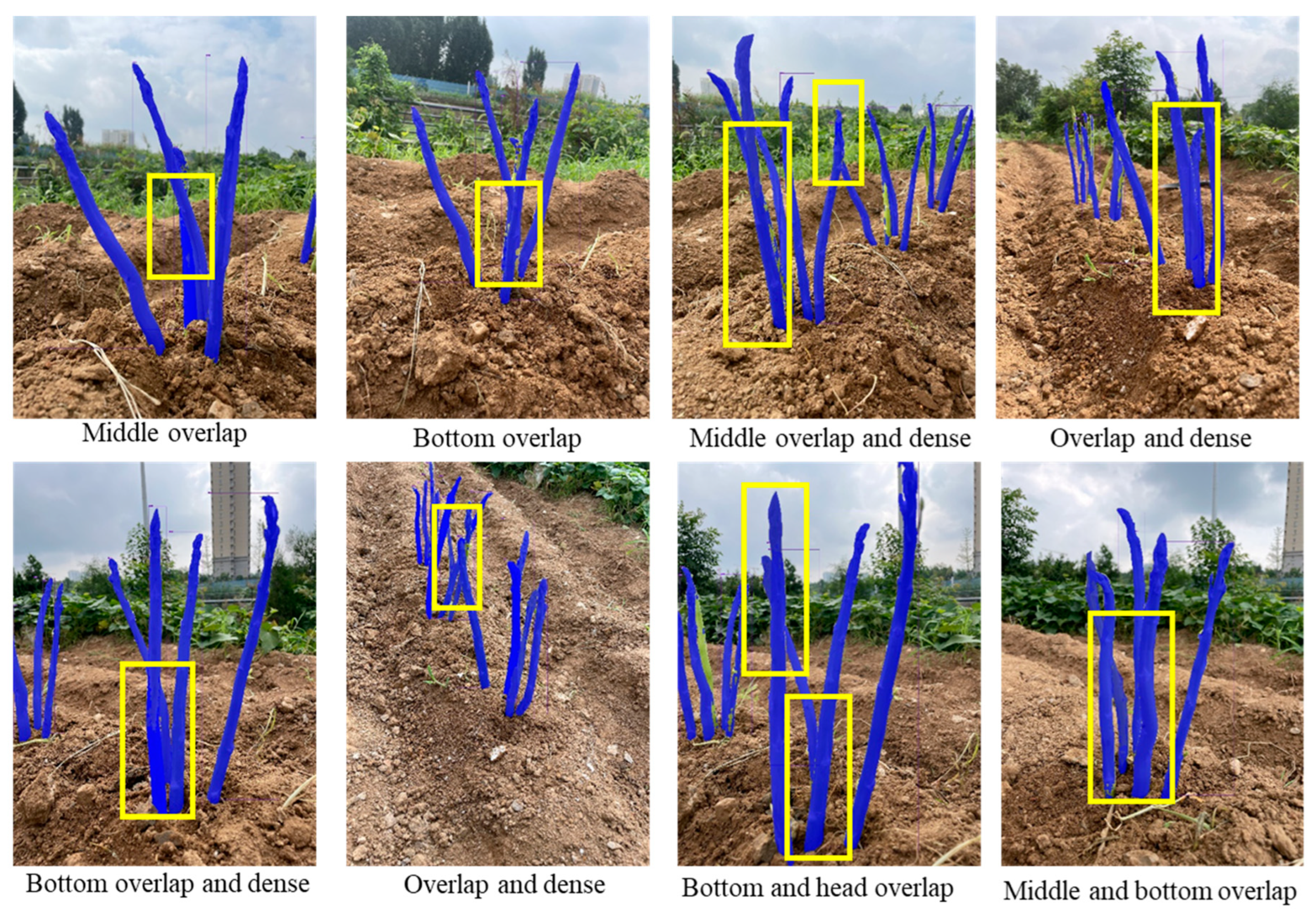
The data of green asparagus in this paper was acquired in July 2024, which was not the harvest period of green asparagus. Therefore, green asparagus grown outdoors was transplanted to two experimental farms at Panhe Campus of Shandong Agricultural University for outdoor simulation experiments. The images data used in this paper were acquired using an RGB-D sensor, RealSense D435i (Intel, Santa Clara, America) under both cloudy and sunny weather conditions. The collection periods included 7 a.m. to acquire green asparagus images of the low-light environment, and 5: 30 p.m. to the sunlight slanted. During these two periods, the camera collected a total of 730 original data, including 3182 green asparagus plants. In order to better simulate the visual system during the picking robot operation, we collected the images from multiple directions, and there were many large-area occlusion and coincidence phenomena in the image, including the facts that head, middle, and bottom were occluded. The specific images are shown in Figure 2.
2.2.2. Dataset Preparation
YS3AM was a multi-task network, it was required to detect green asparagus prediction box, key points, and their 3D positions. There were two types of data or dataset, namely RGB-D data, and point cloud data. The RGB-D data was obtained by camera directly. The RGB-D data was four-channel, the R, G, B channel for green asparagus segmentation and KeyPoints detection, and the key points on RGB image as an index in the depth image to read depth value. This point cloud data was used to evaluate the model performance of 3D reconstruction.
- (1)
- Labelling bounding boxes and Data augmentation
During the dataset creation phase, all target green asparagus in RGB images form RGB-D data were labeled using LabelImg v1.8.1 (https://github.com/tzutalin/labelImg), excluding those with occlusions exceeding two-thirds. To enhance the persuasiveness of the experimental results, this paper employed Augmentor and Imgaug (Bloice et al., 2017) to expand the dataset. Given the uneven outdoor terrain and the potential for blurring due to equipment movement, techniques like chamfer, gamma transformation, dilation, and Gaussian noise were used to realistically simulate the growth environment. The datasets were collected in sunny and cloudy conditions, and effects like rain, snow, fog, and clouds were added to simulate various weather scenarios, increasing dataset diversity. Six augmentation methods were randomly applied to single images (Figure 3), resulting in the Sunny dataset expanding from 388 to 2,328 images, totaling 10,488 green asparagus, while the Cloudy dataset grew from 342 to 2,052 images, containing 8,604 green asparagus. Both datasets were randomly divided into training and testing sets in a 3:1 ratio, with the details shown in Table 1. To reduce training complexity, the resolution of training images was adjusted to 640×640.
- (1)
- Generating color point cloud
The point cloud data was generated by RGB image, internal parameters of camera, and depth image. The coordinate value (u, v) in the pixels coordinate system were used to find the depth value z on the depth image, and the Equation (1) was used to deprojecting and calculating the coordinate value (x, y, z) in the camera coordinate system. And K is a 3×3 matrix containing the internal parameters of camera.
When all pixels were processed as above, a point cloud was generated. This full point cloud is just used to evaluate the results of 3D model detection. For effective consideration, during detection, only the (x, y, z) of some Key-Points in green asparagus was calculated. The subsequent 3D model results are described in the following chapters.
2.3. The Prediction Box Detection of Green Asparagus Stem
In the top-down detection mode, the small image containing a whole asparagus stem must be acquired. And the segmentation results of stem are highly dependent on the prediction box detection results. In the natural environment, the background interference is very strong. Therefore, the prediction box detection network must have a strong background exclusion ability.
Based on the application of the target detection algorithm mentioned in Section 1 in agriculture, the YOLO series network has a strong real-time detection speed. YOLOv7 (Bochkovskiy et al., 2020) is one of the most advanced single-stage target detection algorithms, which balances the conflict between the number of parameters, computational consumption, and performance, and achieves speed and accuracy in satisfactory results in terms of both speed and accuracy (Wang et al., 2022). In this paper, YOLOv7 served as the primary benchmark architecture, and a new design idea was proposed to solve the problems such as the large number of targets under the vision, the different shapes and sizes of stem at each growth stage, and many large-area occlusion and coincidence phenomena in the actual detection application. The Specific improvements from the following four aspects:
- (2)
- The lightweight CBH-S module
The SiLu function of the CBS convolution block in the original model, also known as Swish activation function, is an adaptive activation function. The Swish activation function has the characteristics of no upper bound and lower bound, smooth and non-monotonic, which improves the accuracy of the original model to a certain extent and alleviates the problem of gradient disappearance. However, the Swish activation function has high computational cost, complicated derivation and slow computation in quantization. The CBH-S module was constructed to alleviate the computational cost while ensuring the accuracy of the model. The HardSwish activation function was used to replace the Swish activation function, which was improved on the Swish basis, and reduced the computation by using the segmented linear function to replace the exponential type Sigmoid function with the ReLU6 function. The calculation process is shown in Equation (2).
- (3)
- Heavily parameterized ultra-lightweight feature extraction module
Feature reuse has been a key technique in lightweight convolutional neural network design. The MobileOne ultra-lightweight network module (Anasosalu Vasu et al., 2022) was used to replace the ELAN module of the YOLOv7 backbone to achieve heavy parameterization and ultra-lightweight network architecture.
Using MobileOne (Figure 4) to construct the YOLOv7 backbone network, it was able to extract more rich feature information of green asparagus from the shallow layer of the network, including the cases of not being occluded, roots being occluded, and green asparagus spears being occluded. During the network training process, the deep convolution of MobileOne made it possible to obtain a larger sensory field at different scales by 3×3 convolution kernel. By constructing multiple paths on different levels, each channel of the detected green asparagus feature map had certain information exchange, and the feature information of the lower layer is complemented with the richer feature information of the previous layers.
- (4)
- Lightweight Multi-path Convolution
In the past, attention mechanism only considered the encoding inter-channel information and ignored the importance of location information. Hou et al. Hou et al. (Hou et al., 2021) proposed a novel mobile network attention mechanism for lightweight networks, which embedded location information into channel attention, called CoordAttention (CA) .
The down-sampling process in the feature fusion stage has two transition modules MPConv. The improved MPConv structure is shown in Figure 5b. The plug-and-play CA attention mechanism was replaced the 1x1 convolution of the second branch of the MPConv module, which could reduce both the feature loss caused by the network feature processing and the computational overhead of the mobile device by accurately locating and identifying the target area. At the same time, a CBH-S convolutional module with step size of 2, 3×3 and a CBH-S convolutional module with step size of 1,1 ×1 was used to replace the Conv module, which could reduce the calculation amount and ensure the model had a better performance.
- (5)
- Cross-Scale Integration Strategy
Multi-scale fusion feature can capture the details and features of target objects at different scales and improve the performance of target detection and recognition tasks. Based on the growth pattern of green asparagus in clusters and the influence of the surrounding environment, in order to improve the feature extraction ability of the network for green asparagus, as well as the adaptability to light changes and scale changes, the cross-scale fusion feature diagram of the feature fusion layer and backbone layer was proposed in this paper, as shown by the red dashed arrows in Figure 6.
The stems of green asparagus grown in outdoor have features such as occlusion and overlap, and when two green asparagus are very close together, they can be easily mistaken as one object or similar objects. This strategy could expand the model acceptance field through cross-scale connection, and fused the target features obtained in the shallow feature extraction stage with the semantic information of the deep network, which could learn more detailed features during the fusion process.
The overall improved YOLOv7 model is shown in Figure 6.
Figure 6.
The improved YOLOv7.
2.4. Image Segmentation Network Architectures for Green Asparagus
After the improved YOLOv7 detected the RGB images acquired by the depth camera, the prediction boxes of each asparagus could be obtained, and then, the Segment Anything Model (SAM) was used to detect and segment green asparagus stem clusters.
SAM (Dosovitskiy et al., 2020; Kirillov et al., 2023) is a large-scale model of an innovative model developed by Facebook Research in 2023 for general segmentation tasks in computer vision. Trained on a large dataset, SAM can segment (cut-out) any morphological feature in any given image identifying which pixels belong to an object. The SAM comprises a vision transformer-based image encoder, a prompt encoder, and a lightweight mask decoder. The image encoder consists of a mask-based autoencoder (He et al., 2021) and a pre-trained vision transformer model (Dosovitskiy et al., 2020). Prompt Encoder (Prompt Encoder) has two categories: sparse (points, boxes, text) and dense (mask). Points and boxes can be represented by location coding, which combines learning embeddings from each prompt and arbitrary forms of text (processed using a multimodal pre-trained neural network CLIP). The mask is then combined with the image elements after being embedded by convolution. The lightweight mask decoder can effectively map image encoding, prompt encoding, and output token tokens to the mask. The decoder of the SAM model is based on the decoder block of Transformer, and the dynamic mask prediction head is added after the decoder. The modified decoder block uses prompt self-attention and cross-attention in both the prompt-to-image embedding and vice-versa directions. After running both blocks, the image coding is up-sampled and then the output labeled tokens are mapped to the dynamic linear classifier using MLP. And finally, the dynamic linear classifier calculates the mask prospect probability for each image location.
The transfer learning was utilized to test the detection boxes obtained by the improved YOLOv7 with the weights generated by the base segmentation model SAM on the SA-1B dataset without additional training. The chosen task was semantic segmentation, i.e., dividing the pixels of each image into two different semantic categories: green asparagus (foreground) and background. The process of recognition, and semantic segmentation for a natural color image of outdoor green asparagus captured by depth camera (Intel RealSense D435i) is shown in Figure 7. Although SAM was not specifically trained for the green asparagus image, SAM captured all the major features in the image, which demonstrated its effectiveness. In addition, accessing the geometric features of Mask allowed for further feature extraction of green asparagus.
2.5. Extracting Space Coordinates for Green Asparagus Stem Using Pixel Mapping
After segmenting green asparagus in the images, the SAM model output their binary mask and mapped it to the corresponding depth image to determine the area where the target was located. However, the initial depth data obtained in the unstructured environment was often mixed with noise and pixel information loss. The dense and noisy initial depth image must pass through a series of preprocessing steps before being used for subsequent analysis and calculations.
2.5.1. Mask-Based Deep Pixel Block Completion
Due to the limitations of the RealSense D435i, the output depth maps suffer from issues like reflections, semi-transparent and dark objects, and out-of-range measurements. These factors result in missing depth image pixels and noise, affecting the ability of the green asparagus harvesting robot to establish a complete working space. Therefore, referred the IP_BASIC method(Ku et al., 2018),and employed improved pixel dilation to fill in the missing pixel blocks in the depth data, thereby reducing the complexity of subsequent work and improving the accuracy of the algorithm. The specific process is as follows:
- (1)
- The depth camera was positioned forward to capture outdoor images of green asparagus. A distance threshold of 2 meters was set to filter out distant background, and the depth images were aligned with the RGB images (Figure 8b).
- (2)
- The captured RGB images were automatically segmented to create masks for each green asparagus. A pseudo-color was added to the depth map, which was then converted from RGB to HSV color space, separating the H, S, and V components into three independent grayscale images (Figure 8c). Due to light interference, the V component was chosen to eliminate darker and oversaturated pixels.
- (3)
- The mask images for each green asparagus undergone erosion with a 3×3 elliptical kernel to reduce fine noise and details at the edges (Figure 8d).
- (4)
Figure 8.
Pixel Block Completion for depth image.
The pseudocode for pixel block completion is presented in Table 2. The RGB image (RGBimg), depth image (Depthimg), and mask image (Maskimg) were obtained from the RGB-D sensor. The YS3AM algorithm processes RGBimg to generate Maskimg. The Depthimg was converted to HSV space (Depth_hsv_img), and the V channel was selected to create the processed depth image (Processed_Depthimg). Next, the maximum iteration count (Max_Iterations) and threshold (Threshold) are defined, and Processed_Depthimg was assigned to a temporary depth map (tempDepthMap). For each pixel (i, j) in Depthimg that is null, it checked whether Maskimg[i][j] was marked as an object (OBJECT). If it was, the neighboring pixel values (neighbors) were retrieved, and valid depth values (validDepths) were filtered out. A function named reduce_noise was created to apply erosion to the mask image. Another function named fill_missing_pixels was created to fill in the missing pixels in the depth image using dilation. If the maximum difference between tempDepthMap and Depthimg was less than Threshold, the loop exits. Finally, the processed depth map (completedDepthMap) was returned.
2.5.2. The Positional Transformation Relationship of Spatial Points of Clustered Green Asparagus
Before establishing the mapping relationship between the 2D images and the depth image, the camera was calibrated to obtain its internal and external parameters, such as the focal length, translation vector, and rotation matrix.
First, an image RGB-D image was split into a RGB image, and a depth image. In Figure 1, the RGB image (Figure 1a) was fed in the detect network (Figure 1b), and the prediction boxes of stem were generated. The evaluation metrics and results of prediction box detection was shown in Section 3.1. Then, according to these predicted prediction boxes, each small image contains one asparagus stem was fed into SAM to segment the green asparagus stem from the background. Finally, the contour of green asparagus in pixel coordinates could be obtained through OpenCV. Because the depth image was aligned to the RGB image, the pixel coordinates (U, V) of the contour on the image could be used as the index to find the corresponding depth value.
The mapping relationship between the 2D image and depth image can establish the spatial mapping relationship between the pixel and camera coordinate systems. Based on the principle of binocular visual localization, we used the depth camera intrinsic parameters to convert the contour area detected by the model to space coordinates. The mapping relationship is expressed as follows:
where (xi, yi, zi) are the 3D coordinates of pixel i in camera coordinates; (ui, vi) are the pixel coordinates of pixel i; D is the depth image; is the depth scale factor of the camera; (Ux, Uy) are the pixel coordinates of the IR camera principal point; and (fx, fy) are the focal lengths of the IR camera. The positional relationship of spatial points in the camera coordinate system is shown in Figure 9.
2.6. Adaptive-section modeling of clustered green asparagus stems
2.6.1. Visual 3D Section Modeling Approach
Rapid 3D modeling of green asparagus is crucial for efficient harvesting path planning. However, the varying thicknesses, tilting postures, and bending directions of the stems can lead to excessive computational demands if modeled too precisely, impacting efficiency and speed. Voxel modeling offers a more efficient solution by using fixed-length cubes to represent spatial point clouds. Given the upward growth and simple structure of green asparagus, voxel-like geometric modeling is ideal for balancing efficiency and accuracy. We used a cylindrical structure as the basic element, dividing each asparagus into N sections and combining these cylinders to create a precise 3D model of clustered asparagus. This approach lays the groundwork for effective harvesting planning.
As shown in Fig.10, through the network structure mentioned earlier, clusters green asparagus could be identification and localization and semantic segmentation, and the mask of each green asparagus could be detected by prediction boxes. The binary mask images were instrumental in extracting stem parameters, including the 2D coordinates of the bottom, the tip and the key point of the asparagus stem. These coordinates served as the projection of the three-dimensional object on the camera plane. Utilizing the alignment capabilities of an RGB-D sensor, these 2D coordinates were fused with depth information to determine the depth Du,v of the point Pu,v in the camera space. The Du,v was then converted to obtain the Z-axis coordinates in the camera coordinate system, yielding the spatial position information P (x, y, z) of point P.
For example, when dividing a stem into N cylindrical sections, each cylinder Ci had a radius Ri and length Li, represented as ∪Ci (Ri, Li). Given the stems’ inclination and curvature, each Li was calculated from fused depth data in the mask image, ensuring modeling accuracy. Specifically, the length Li of green asparagus was derived through mask and depth images, coordinate transformation, and spatial line fitting, then averaged into N sections with each segment length Lci/N. The radius Ri was similarly derived from the depth-fused mask. In camera space, the mask determined the bottom surface position of each Ci, with coordinates of both ends obtained from the bottom cutoff line in the mask image. Converting depth to camera coordinates gives world coordinates for each endpoint and a point on the cutoff line. Finally, Ci was fitted to find its center Oi (xoi, yoi, zoi) and Ri in cross-section, accurately positioning and linking each cylinder
Figure 10.
Schematic diagram for 3D section modeling of stems (e.g.: 6 equal sections).
The pseudocode for the section modeling of clustered green asparagus stems is presented in Table 3. Firstly, the RGB-D sensor acquired the RGB image and the Depth image, which were stored as RGBimg and Depthimg, respectively. Through the YS3AM proposed in this paper, target recognition, segmentation, and semantic information extraction were conducted on the RGBimg. The recognition boxes and masks were stored in Boxes and Maskimg respectively. Secondly, for each selected box each in Boxes, the SeparateAsparagus function was constructed to separate each green asparagus in Maskimg. The GetKeyPoint function was constructed to extract the key point coordinates of the top, bottom, left, and right of each green asparagus. The Calculate_L function was constructed to calculate the length of the asparagus. Thirdly, the green asparagus was divided into N sections. For each section i, the bottom position BottomPos of Ci was calculated. The Calculate_R and GetCenterPoint functions were respectively constructed to calculate the radius and center point of Ci based on each BottomPos. Finally, the MapPostoCamere function was constructed to convert the center point, length, and radius of Ci into camera coordinates (x, y, z) and plot Ci using the PlotCylinder function. This process was repeated until the modeling of the clustered green asparagus was accomplished.
2.6.2. Parameter Calculations of Section Modeling
(1) Length calculation of each section
To determine the length of the asparagus stem, this paper employed a scheme of fitting the outline curve of the asparagus stem. We first segmented the green asparagus within the prediction box using the SAM model. This segmentation allowed us to identify and isolate each individual asparagus stem, and obtain the contour of each green asparagus. Then, we addressed some missing pixels in the depth image using the method described in section 2.5.1. This process ensured that we had a complete and accurate depth image. Scanning each pixel point on the contour, the 3D coordinates (x, y, z) of each pixel point in the camera coordinate system were calculated using the method outlined in section 2.5.2, which provides a reliable way to transform the 2D pixel coordinates into their corresponding 3D spatial coordinates. Finally, to create a smooth and accurate representation of the asparagus stem, we fitted a spatial curve line to the pixel points on the contour. The spatial linear equation is fitted according to the least squares method:
where, (x0, y0, z0) is any point on the contour and (m, n, p) is the direction vector on the fitted line. An equivalent transformation of the above equation can be expressed as:
where,
Based on the principle of least squares fitting, the space curve equation fitted to the green asparagus can be expressed as:
where,
To determine the length of each approximate cylinder along the fitted line of the green asparagus stem, we needed start by identifying the top point and the bottom point of the stem section. Based on the idea of stem section, the fitted line connecting these two points was evenly divided into N section s. The length of each approximate cylinder section was the Euclidean distance between the endpoints of each section. For two spatial points Pi and Pi+1, the distance Li is calculated as:
Since the sections were evenly divided, this distance would be approximately the same for each section, Li could be considered the approximate length of the cylinder i. By using this method, we could determine the length of each section of the cylinder that approximates the green asparagus stem (Figure 11).
(2) Center and diameter calculation of each section
Next, it was necessary to calculate the center and radius of the approximate cylinder for each section of the asparagus stem. In the camera coordinate system, we assumed that each section was parallel to the y-axis. We then made m horizontal cuts parallel to the xoz-plane (Figure 12b). Each cut revealed that the intersection of the horizontal section with the cylinder maintained a circular surface. Due to the camera’s shooting angle, we only observed a portion of the arc of the circular surface at a time. To address this, we selected three points Pi1(xi1, zi1), Pi2 (xi2, zi2), Pi3 (xi3, zi3) on the circular arc of an intersecting circular surface (Figure 12c). Using these points, we determined the center o′ (xio, zio) of the circle that the arc belonged to, as well as its radius (r). The specific calculation method is as follows:
In Equations (6)–(8),
Based on the above equations, we could then construct the binary function on the radius (r), defined as:
From the definition of the limit of a binary function, all points Pi (xi, zi) on the visible arc should satisfy:
where, ε represented a given positive number, so A was the limit of when . Specifically, A corresponded the radius (r) of the circle in which the arc lied and o’ (xio, zio) was the center of the circle. After these calculations, we were able to determine the base circle (center: o’ (xio, zio) and radius: r) and length of each stem section.
Figure 12.
Calculating the width of each stem.
2.6.3. Section Modeling Accuracy Assessment Methods
The differences in the thickness and inclination angle of the stem will inevitably cause differences in the accuracy of section modeling. The accuracy of 3D modeling is usually measured by the RMSE (Root Mean Square Error) index, which is a commonly used indicator to measure the accuracy of prediction models. It is used to measure the degree of difference between the predicted value and the actual observed value, i.e.
where, is a point on the section cylinder, is the real measured value of a point on the shoot, and n is the number of samples. For the section number N, the RMSE index is statistically calculated for each section, and RMSEi is the index value of section Ci. The maximum value of RMSE is taken as the indicator of the modeling accuracy of the entire green asparagus stem, i.e., MAX(RMSEi).
When computing the RMSEi of the Ci section, theoretically, it is necessary to perform calculations for all points in space and those on the section cylindrical surface. However, this approach would reduce computational efficiency and is unnecessary, as RGB-D sensors can only collect depth information from one side, leaving the back of the asparagus stem invisible. Thus, it is impossible to obtain the complete 3D information of the asparagus stem, and it is also infeasible to take all points as the basis for calculating RMSE. Analyses reveal that assuming the cross-section of the green asparagus is circular, using the maximum offset as an indicator, the offset of the stem can be replaced by the axis offset. Therefore, finding the MAX(RMSEi) is equivalent to determining the offset of the cross-sectional center. We accelerated the calculation of the RMSEi index for each Ci section by using a small number of typical values instead of all points. These points consisted of the centers of the cross-sections passing through specific positions on the stem, including the extreme points on the depth map and the inflection points on the contour of the mask image.
The pseudocode in Table 4 illustrates the process for computing modeling indices of each green asparagus section. Correspondingly, the RGB image (RGBimg) and depth image (Depthimg) were acquired from the RGB-D sensor. Semantic extraction of RGBimg was performed using the YS3AM framework proposed in this paper, with masks subsequently stored in Maskimg. The sequences for KeyPoints and ModelPoints were initialized accordingly. To identify all extreme points within Maskimg and Depthimg, a function named findExtremePoints was developed to store these points in SpecialPoints. Additionally, two functions—CalculateCenter and MapModelCenter—were constructed to compute both the true cross-sectional centers and their corresponding model cross-sectional centers mapped to identical positions. And these results were recorded in KeyPoints and ModelPoints respectively. Following this, RMSE_Ci was then calculated by iterating over variable points, with the maximum RMSE across sections serving as the overall evaluation index for the asparagus stem.
2.6.4. Calculation of the Section Count for Adaptive Modeling
Variations in length, thickness, and posture among asparagus stems lead to differences in modeling accuracy when a fixed number of sections NNN is used uniformly. However, accurate and consistent modeling across all stems is essential for subsequent path planning and end-effector motion control. Therefore, selecting an appropriate number of sections for each stem is crucial. This paper introduced an adaptive-section modeling methodology focused on clustered green asparagus stems based on stem length. Specifically, it involved automatically selecting the number of sections according to stem lengths to ensure consistent modeling accuracy for all stems within the camera’s field of view. Assuming that the length of an intact stem was L and defining parameter n as the section count, we outlined expectations for different stems as follows:
where, P denoted the model accuracy evaluation function, Cs=∪Ci (Ri, Li) represented the N- section model, As referred to the artificially collected empirical data, and signified the allowable accuracy. Assuming that the positioning accuracy of the actuator was not taken into account, ε could be derived from the measurement precision of the RGB-D sensor. During practical measurements, due to the irregular surface of stems, the depth measurement error of the RGB-D sensor under illuminated conditions was 5 mm. Thus, could be approximated as =5×10⁻³. It was evident that n should be a function of asparagus stem length L. An increase in n correlated with enhanced modeling accuracy and greater model fidelity. However, a larger value for n also resulted in increased computational complexity. Therefore, for different asparagus stems i and j, there should be:
where, i, j∈N. The result of the function P determined the accuracy of the visual model of green asparagus, depending on the calculated values of the evaluation indicators in Section 2.6.3.
The pseudocode for calculating the adaptive modeling section count of asparagus stems is provided in Table 5. An iterative methodology was employed to ascertain the optimal number of section s. For green asparagus i, =5×10⁻³ was initialized as the termination criterion for iteration, and the initial section count was set to N (this paper beginned with N = 4). The CalculateP function was developed to compute the RMSE value of 3D modeling when the section counted equal 4, followed by an assessment of whether the modeling accuracy requirements was satisfied. If not, an iterative loop commences wherein the section count was incremented by one until satisfactory modeling accuracy was achieved. The resultant section count represented the optimal segmentation that meet the specified accuracy criteria.
3. Experimental Results
The multi-task network in YS3AM was a cascade of two networks, prediction box detection and mask segmentation. During prediction, these networks were interconnected in a head-to-tail configuration, resulting in an output that delineates the contour of asparagus stems within the full image. Therefore, both the structure of the network and its combination had an influence on the final visualizing the spatial location of each green asparagus. The comparative experiments were designed to select the best combination of networks. This encompassed the presentation of model recognition and segmentation results, ablation experiments assessing the detection accuracy of green asparagus using various improvement strategies. Furthermore, this paper validated the accuracy of the proposed adaptive spatial segmentation model for green asparagus. These included evaluations of key-point offset testing, measurements of stem length and width errors, and Laboratory Farm random stalk assessment.
The detection network in this paper was implemented using the Pytorch framework, the specific hardware configuration and experimental setup are detailed in the following Table 6.
3.1. Evaluation Metrics
This paper evaluated the performance of each group by comparing the precision, recall, F1 score, loss function, and detection time. Specifically, the Precision was defined as the ratio of the number of correct identifications of green asparagus on the image to the total number. The Recall was the proportion of correctly detected green asparagus to all green asparagus that should be detected. The F1 score was the harmonic mean of Precision and Recall, and it provided a balanced evaluation of a model’s performance. Additionally, the number of parameters represented the total count of parameters. The gradient was the maximum rate of change of the function along the gradient direction. GFLOPs represented the number of floating-point operations required for model inference.
This paper utilized binocular stereo vision technology to perform the localization and segmentation of clustered green asparagus, while also developing a 3D model for adaptive-section based on stem length. Inevitably, discrepancies arise between the actual positions of outdoor crops and their predicted locations, leading to deviations in the constructed visualization model from real-world conditions. Consequently, when assessing the green asparagus model, evaluation metrics such as the coefficient of determination (R²), root mean square error (RMSE), and Pearson’s correlation coefficient were recommended.
3.2. Model Performance Test
3.2.1. Detection and segmentation results
YS3AM could identify green asparagus under conditions of light variation, complex backgrounds, and interwoven overlaps, showing good recognition and segmentation results. In this section, we validated the recognition results of YS3AM using the Sunny and Cloudy datasets, as well as the total dataset of all images, following the method described in Section 2.4. Table 7 presented the detection results for the total dataset, including various metrics (Precision, Recall, F1, and mAP) at different confidence levels. Figure 13 illustrated a comparison of the various mAP and loss obtained by all models trained with images from the Sunny, Cloudy, and Total datasets (IoU = 0.2, Conf = 0.6). It could be observed from the figure that the mAP value (0.972) using the Total training set images was slightly higher than that of Sunny (0.966) and Cloudy (0.961). The box-loss (0.036) for the Total dataset images was higher than for Sunny (0.024) and Cloudy (0.028). The overall model performance was stable, with the obj-loss (0.068) being slightly higher than that of Sunny (0.021) and Cloudy (0.024), and the mIOU (0.874) was lower than Sunny (0.913) and Cloudy (0.900). After comparison, the overall performance of YS3AM was stable.
However, the overall metrics showed that the detection performance on the Sunny dataset was superior to that on the Cloudy dataset. Binocular stereo vision methods rely on natural light in the environment to capture images and is very sensitive to ambient lighting conditions. Due to the influence of environmental factors such as changes in light angle and light intensity, the brightness difference between two images captured by the depth camera is relatively large, which presents a considerable challenge to matching algorithms. The mAP detection rate for the Sunny dataset was 14.29% higher than that for the Cloudy dataset, the box-loss detection rate was 16.67% higher, the obj-loss detection rate was 2.52% lower, and the mIOU was 1.42% higher. Figure 14 illustrated the recognition and segmentation effect of our model on clustered green asparagus under different lighting conditions, such as dense, overlapping and occlusion, and the detection and segmentation accuracies of model were high.

Table 7.
Detection results of the total dataset for different confidence levels (IoU threshold set to 0.2)).
Table 7.
Detection results of the total dataset for different confidence levels (IoU threshold set to 0.2)).
| Conf | Precision (%) | Recall (%) | F1 | mAP (%) |
| 0.5 | 98.35% | 95.14% | 0.967 | 96.84% |
| 0.6 | 98.75% | 95.46% | 0.971 | 97.16% |
| 0.7 | 98.36% | 95.31% | 0.968 | 96.77% |
| 0.8 | 97.76% | 95.54% | 0.966 | 97.07% |
| 0.9 | 98.44% | 95.54% | 0.969 | 96.89% |
Figure 13.
Evaluation metrics for models on the three datasets.
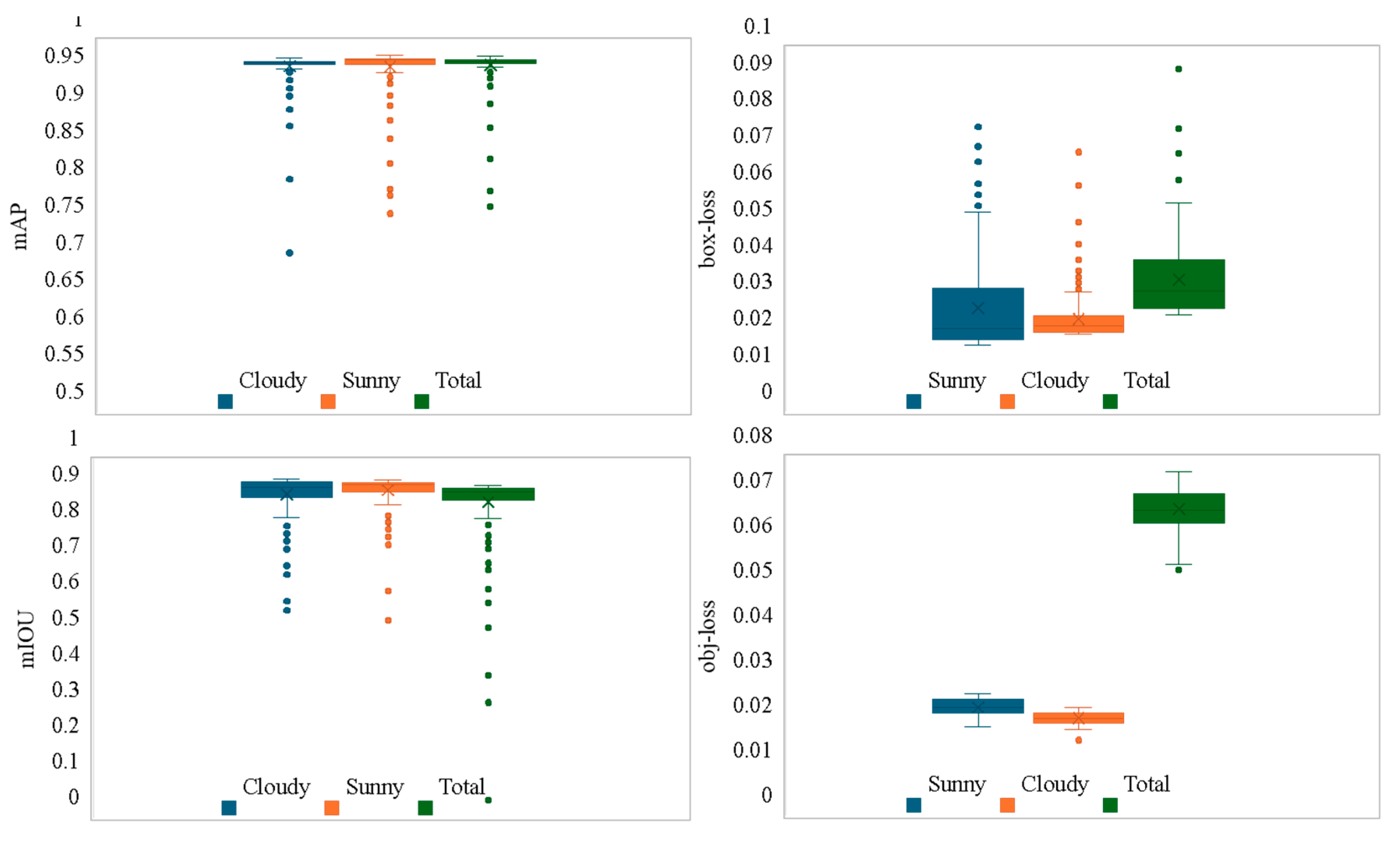
Figure 14.
Detection and Segmentation result of green asparagus. The overlaps of asparagus stem are marked with yellow boxes.
Figure 14.
Detection and Segmentation result of green asparagus. The overlaps of asparagus stem are marked with yellow boxes.
3.2.2. The Results of Ablation Studies
As previously mentioned, we made four main improvements to the original YOLOv7, including some structural changes to the network (e.g., lightweight CBH-S module, MobileOne ultra-lightweight module for obtaining a larger receptive field at different scales, lightweight down-sampling module (CAConv) that focused on location information, shallow -to-deep cross-scale fusion architecture). Therefore, we further performed ablation experiments to determine which modification contributed the most to the proposed YS3AM network, which leaded to better detection capability in this work. Model A represented the original YOLOv7 model, while models B to J represented varying degrees of improvement to model A under the most optimal hyperparameters. Model B implemented a lightweight model that replaced the CBS module with the CBH-S module. Model C implemented a lightweight MobileOne replacing the ELAN module of the YOLOv7 backbone. Model D implemented the use of lightweight CAConv modules that combined locational information and attention mechanisms to replace the MPConv module in the Neck section. Model E achieved multi-feature extraction from deep to shallow layers through cross-scale fusion. Model F was the fusion of models B and C, achieving multi-level feature extraction on the basis of lightweight. Model G was the fusion of models B, C, and D, achieving multi-path information fusion while being lightweight. Model H was the fusion of models B, C, and E, achieving lightweight cross-scale fusion. Model I was the fusion of models B, D, and E, achieving multi-information fusion across scales. Model J was the improved model proposed by us. Table 8 shows the results of the ablation study, which clearly indicates that these four structural improvements are beneficial to the performance of YS3AM. As expected, YS3AM performed the best in the ablation study because it combined structural and attention modifications.
As shown in Table 7 and Figure 15, the Precision of the YS3AM model is the highest, the YS3AM model achieved the highest Precision. Although the Recall of model was 0.07 percentage points lower than Model E, the F1 score remained superior to other models. The mAP of the YS3AM model was marginally lower than that of Model E, which suggested that cross-scale fusion methods could adequately capture the complex target in the model down-sampling process (e.g., stem interlacing) features. The cross-scale fusion strategy provided a more comprehensive understanding of the data. Replacing CBS with CBH-S further improved the metrics, and the total Loss of the model was reduced by 50.65%, reflecting the stronger generalization ability of the lightweight module. With the different modules introduced in YOLOv7, there was a relatively significant and proportional decrease in the computation of the model, especially with Model H being the lowest. This also illustrated the substantial contribution of lightweight structures to our model. Therefore, although all the above models were based on the YOLO architecture and had achieved good results in some cases, they were not generalizable and require special algorithms to be designed for different datasets and practical needs. The effectiveness of the YS3AM model in recognizing green asparagus growing in clusters outdoors was verified by comparing it with the above models.
3.3. Assessment of Spatial Information Visualization in Green Asparagus
3.3.1. Key-Point Deviation Detection Test Results
An experiment was performed in a laboratory environment to determine the optimal number of sections for the visualization model. Four set of 12 green asparagus (Figure 16) were used as targets for this test. The length standard for harvesting the stems of green asparagus varies according to the purpose. If used as raw materials for processing, the harvest is carried out when the stems reach a length of 14~21 cm. For domestic market sales, a length of 25~28 cm is appropriate. And for the winter market in the northern regions, the length of the asparagus stems is about 30~35 cm. Therefore, the length intervals we select are as follows: 15~20 cm, 21~25 cm, 26~30 cm, and 31~35 cm.
The targets were fixed in a vertical position. The camera was mounted on a tripod about 35-40cm from the test targets (Figure 17). In this paper, a section testing approach was adopted. Each green asparagus was equally divided into 4, 6, 8, and 10 sections respectively, and each section of the asparagus stem could be approximated as a cylinder. Furthermore, we selected certain key points on the edge of the bottom surface of each cylinder (including the leftmost, center, and rightmost points), and calculated the average RMSE of the predicted and point cloud true depths of each key point in different section methods in accordance with the precision evaluation method in 2.6.3. All RMSE results of the key-point test are summarized in Table 9. The section model is shown in Figure 18.
As could be seen by comparing Table 9, when exploring the optimal number of sections, both the MAX(RMSEi) and the limit of the maximum error needed to be taken into consideration. Firstly, for the three green asparagus stems with lengths ranging from 15 to 20 cm, the MAX(RMSEi) existed when No. 1 and No. 2 were equally divided into 4 sections; for No. 3, the MAX(RMSEi) existed when it was equally divided into 8 sections. Since the maximum error should not exceed =5×10⁻³ during the optimal section, the accuracy of No. 3 was the highest when it was equally divided into 4 sections. Then, observing the RMSE results of the three green asparagus stems with lengths ranging from 21 to 25 cm, the visualization model had the highest accuracy when No. 4 was equally divided into 6 sections; for No. 5, although the MAX(RMSEi) existed when it was equally divided into 4 sections, it obviously exceeded the maximum error, thus it was most appropriate to equally divide it into 6 sections; the situation of No. 6 was the same as that of No. 5, and finally it was most suitable to equally divide it into 6 sections. Next, for the three green asparagus stems with lengths ranging from 26 to 30 cm, the MAX(RMSEi) of No. 7 occurred when it was equally divided into 8 sections and did not exceed the maximum error; for No. 8 and No. 9, the MAX(RMSEi) occurred when they were equally divided into 6 sections, but due to the limit of the maximum error, the accuracy was the highest when they were equally divided into 8 sections. Finally, observing the three green asparagus stems with lengths ranging from 31 to 35 cm, when No. 10 was equally divided into 8 sections, it exceeded the maximum error, thus equally dividing it into 10 sections was the best choice; both No. 11 and No. 12 had the MAX(RMSEi) when equally divided into 10 sections and did not exceed the maximum error. The above 12 green asparagus stems could fully cover the length requirements of suitable harvestable green asparagus for different application needs. Therefore, a conclusion could be drawn. That was, green asparagus with lengths ranging from 15 to 20 cm could be equally divided into 4 sections; those with lengths ranging from 21 to 25 cm could be equally divided into 6 sections; green asparagus with lengths ranging from 26 to 30 cm could be equally divided into 6 or 8 sections; and those with lengths ranging from 31 to 35 cm could be equally divided into 8 or 10 sections.
3.3.2. The Length and Width Measurement Results
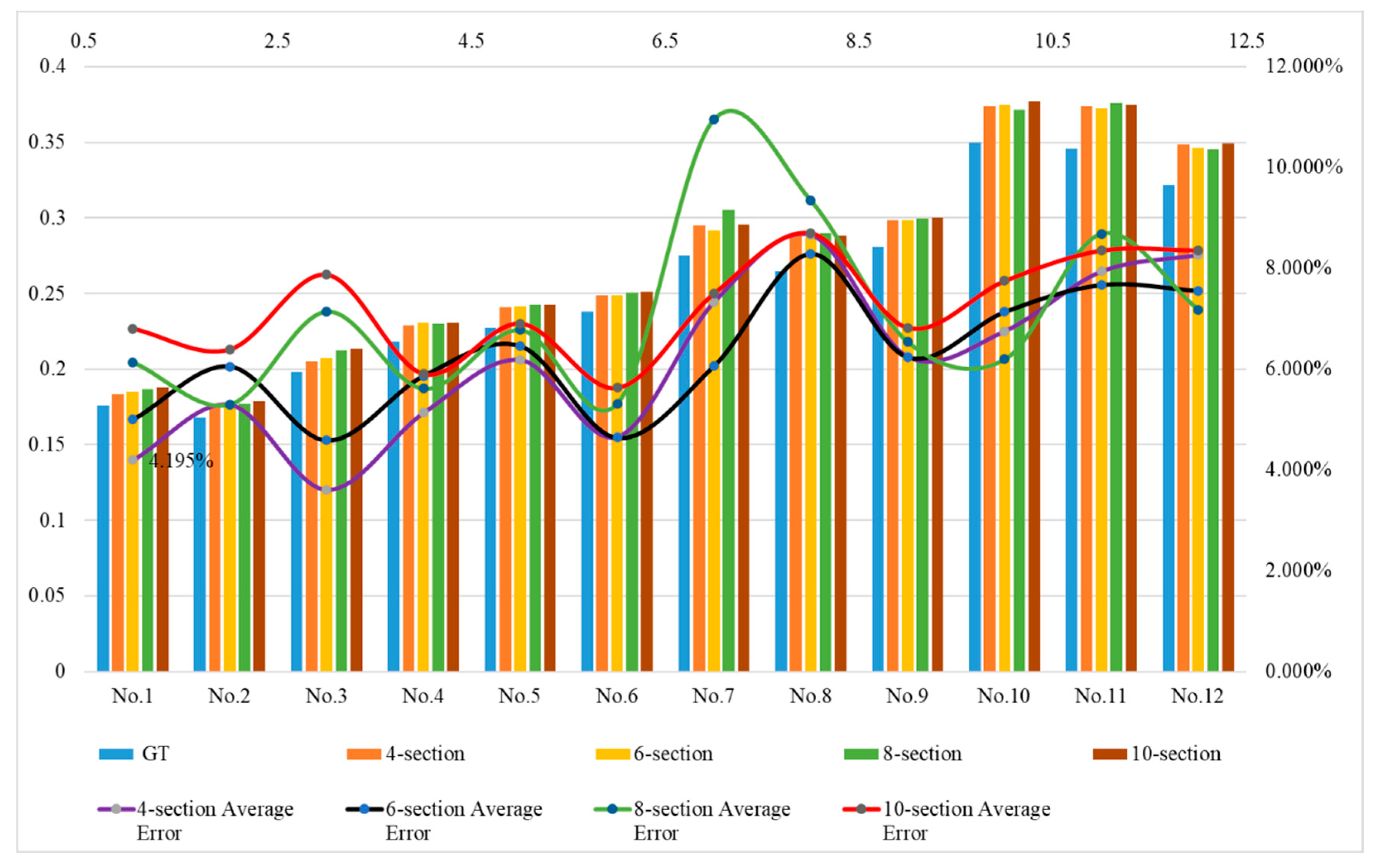
Through visits and investigations of multiple planting parks, mature green asparagus stems typically present an upright state, with a smooth and straight surface. Hence, apart from considering the deviation degree of some key points at the section parts of the asparagus stems, we can also conduct evaluations by judging the errors in the length and width of the stems. The 12 green asparagus stems in 3.3.1 were still subject to testing. All errors of the length test and width test are summarized in Table 10 and Tabel 11, also shown in Figure 19 and Figure 20 for better comprehension.
As it can be seen by comparing Table 11, the length error of the first group of tests was the smallest when divided into 4 equal sections, that of the second group was the smallest when divided into 4 and 6 equal sections, that of the third group was the smallest when divided into 6 equal sections, and that of the fourth group was the smallest when divided into 6 and 8 equal sections. Combining the results of 3.4.1, we discovered that shorter green asparagus could attain higher accuracy with a smaller number of sections. However, for longer green asparagus, a greater number of sections did not necessarily imply higher model accuracy. On the contrary, a larger computational volume would excessively occupy system resources. This result was approximately the same as that of 3.3.1.
Table 10.
Length analysis for different sections of table (unit: m).
| 4-section | 6-section | 8-section | 10-section | |||||||
|
GT (m) |
YS3AM (m) |
Error (%) |
YS3AM (m) |
Error (%) |
YS3AM (m) |
Error (%) |
YS3AM (m) |
Error (%) | ||
| Group 1 | 1 | 0.176 | 0.183 | 4.195 | 0.185 | 5.000 | 0.187 | 6.136 | 0.188 | 6.806 |
| 2 | 0.168 | 0.177 | 5.296 | 0.178 | 6.054 | 0.177 | 5.297 | 0.179 | 6.396 | |
| 3 | 0.198 | 0.205 | 3.607 | 0.207 | 4.584 | 0.212 | 7.140 | 0.214 | 7.878 | |
| Group 2 | 4 | 0.218 | 0.229 | 5.131 | 0.231 | 5.865 | 0.230 | 5.610 | 0.231 | 5.908 |
| 5 | 0.227 | 0.241 | 6.183 | 0.242 | 6.456 | 0.242 | 6.774 | 0.243 | 6.908 | |
| 6 | 0.238 | 0.249 | 4.659 | 0.249 | 4.636 | 0.251 | 5.317 | 0.251 | 5.628 | |
| Group 3 | 7 | 0.275 | 0.295 | 7.335 | 0.292 | 6.065 | 0.305 | 10.958 | 0.296 | 7.506 |
| 8 | 0.265 | 0.288 | 8.662 | 0.287 | 8.285 | 0.290 | 9.339 | 0.288 | 8.701 | |
| 9 | 0.281 | 0.299 | 6.245 | 0.299 | 6.234 | 0.299 | 6.536 | 0.300 | 6.823 | |
| Group 4 | 10 | 0.35 | 0.374 | 6.755 | 0.375 | 7.136 | 0.372 | 6.192 | 0.377 | 7.754 |
| 11 | 0.346 | 0.373 | 7.940 | 0.373 | 7.670 | 0.376 | 8.686 | 0.375 | 8.358 | |
| 12 | 0.322 | 0.349 | 8.267 | 0.346 | 7.552 | 0.345 | 7.180 | 0.349 | 8.360 | |
Abbreviations: GT (Ground True): Actual ground measured length of point cloud; YS3AM: Indicates the length of model testing; Error: Error rate of model and manual measurement error.
Figure 19.
Length measurement result.
As it could be seen by comparing Table 11, the first row indicated the number of sections of each green asparagus. The second row, where Mean (GT) and Mean (Model) respectively denoted the average width measured manually and the average width measured by the model test, and Error Std represented the standard deviation of the error between the two measurement methods. Mean Error represented the ratio of the error between the two measurement results to the true width. By comparing the results from Figure 20a to Figure 20h, the width error of green asparagus ranged between 0.45% and 16%, and the larger the width of the asparagus stem, the greater the error.
The measurement error of the width of each asparagus stem when equally divided into 4 sections was shown in Figure 20a. For short green asparagus, the error produced by the depth camera sensor when detecting the top and bottom points was relatively small (green area, approximately 6% - 8%). Therefore, the position error of the left and right key points of each contour section of the asparagus stem was relatively small. When the detection target was taller, the error of the sensor for the top and bottom points of the asparagus stem increased, inevitably causing an increase in the error of the key points of each section. Moreover, due to the smaller number of sections, the mean error and standard deviation also increase relatively (yellow area, 12%). Figure 20b more clearly reflected that the error increases as the asparagus stem grows, and the trend line of the standard deviation of the width of the asparagus stem showed a gentle growth. This deviation could be explained by the hardware issues of the depth camera sensor itself.
The measurement error of the width of each asparagus stem when equally divided into 10 sections was shown in Figure 20g. The green area indicates that the errors are relatively low (approximately 6% - 8%) on asparagus stalks of different lengths. However, an examination of the standard deviation trend line in Figure 20h revealed no discernible pattern when comparing the section of tall and thick green asparagus with that of shorter specimens, as seen between samples No. 1 and No. 2 versed No. 10 and No. 12. Consequently, this methodology was more advantageous for achieving optimal fitting in tall and thick green asparagus, thereby facilitating the establishment of a more accurate visualization model. Figure 20c to Figure 20f illustrated the errors associated with segmenting the asparagus stems into 6 and 8 equal sections. These results fall within the range observed for 4 and 10 sections. Given the relatively straight morphology of green asparagus stems and their inherent correlation between length and width, it could be inferred that measurements taken for width were essentially consistent with those taken for length.
Table 11.
Width analysis for different sections of table (unit: mm).
| NO | 4-section | 6-section | 8-section | 10-section | ||||||||||||
| Mean (GT) | Mean (Model) |
Error Std |
Mean Error (%) |
Mean (GT) | Mean (Model) |
Error Std (%) |
Mean Error |
Mean (GT) | Mean (Model) |
Error Std (%) |
Mean Error |
Mean (GT) | Mean (Model) |
Error Std (%) |
Mean Error (%) |
|
| 1 | 9.208 | 9.524 | 0.251 | 3.223 | 8.697 | 9.307 | 0.581 | 5.860 | 8.716 | 9.531 | 1.318 | 6.906 | 8.904 | 9.418 | 0.622 | 10.458 |
| 2 | 8.623 | 9.29 | 0.787 | 7.261 | 8.310 | 9.308 | 1.040 | 10.718 | 8.305 | 9.211 | 0.735 | 9.838 | 8.375 | 9.125 | 0.751 | 8.220 |
| 3 | 8.830 | 8.892 | 0.621 | 0.699 | 8.852 | 9.466 | 0.966 | 6.486 | 9.013 | 9.256 | 0.727 | 2.625 | 8.753 | 8.841 | 0.545 | 0.998 |
| 4 | 7.852 | 7.963 | 0.136 | 1.420 | 7.938 | 8.016 | 0.313 | 0.981 | 7.929 | 8.14 | 0.835 | 2.663 | 7.860 | 8.163 | 0.395 | 3.851 |
| 5 | 9.288 | 9.691 | 0.022 | 2.440 | 9.350 | 9.832 | 0.234 | 3.209 | 9.33 | 9.563 | 0.432 | 4.166 | 9.032 | 10.832 | 0.678 | 16.619 |
| 6 | 9.170 | 9.289 | 0.719 | 1.280 | 9.106 | 9.095 | 0.591 | 2.084 | 9.231 | 9.182 | 0.388 | 0.539 | 9.151 | 8.986 | 0.595 | 0.481 |
| 7 | 8.200 | 5.209 | 0.360 | 2.234 | 8.365 | 8.182 | 0.741 | 0.109 | 8.394 | 8.346 | 0.688 | 0.580 | 8.156 | 8.403 | 0.574 | 2.932 |
| 8 | 9.520 | 10.719 | 1.421 | 11.187 | 9.048 | 9.848 | 0.588 | 12.278 | 9.894 | 11.108 | 0.835 | 8.585 | 9.319 | 10.594 | 1.233 | 10.928 |
| 9 | 9.274 | 10.064 | 1.417 | 7.872 | 9.183 | 9.455 | 0.196 | 2.886 | 9.388 | 10.42 | 0.861 | 6.927 | 9.387 | 10.116 | 0.838 | 5.130 |
| 10 | 12.958 | 13.784 | 1.017 | 6.069 | 13.031 | 13.487 | 1.180 | 3.380 | 13.074 | 13.487 | 1.070 | 3.067 | 12.931 | 13.297 | 0.579 | 2.754 |
| 11 | 14.783 | 15.631 | 0.971 | 5.428 | 14.503 | 15.996 | 1.043 | 9.331 | 14.313 | 15.406 | 0.999 | 7.091 | 14.938 | 15.774 | 0.687 | 5.301 |
| 12 | 12.989 | 14.692 | 1.275 | 11.589 | 12.853 | 14.745 | 1.620 | 12.835 | 12.93 | 14.46 | 1.795 | 10.582 | 13.002 | 14.191 | 2.304 | 8.381 |
Figure 20.
Width measurement result.
3.3.3. Field Test Results
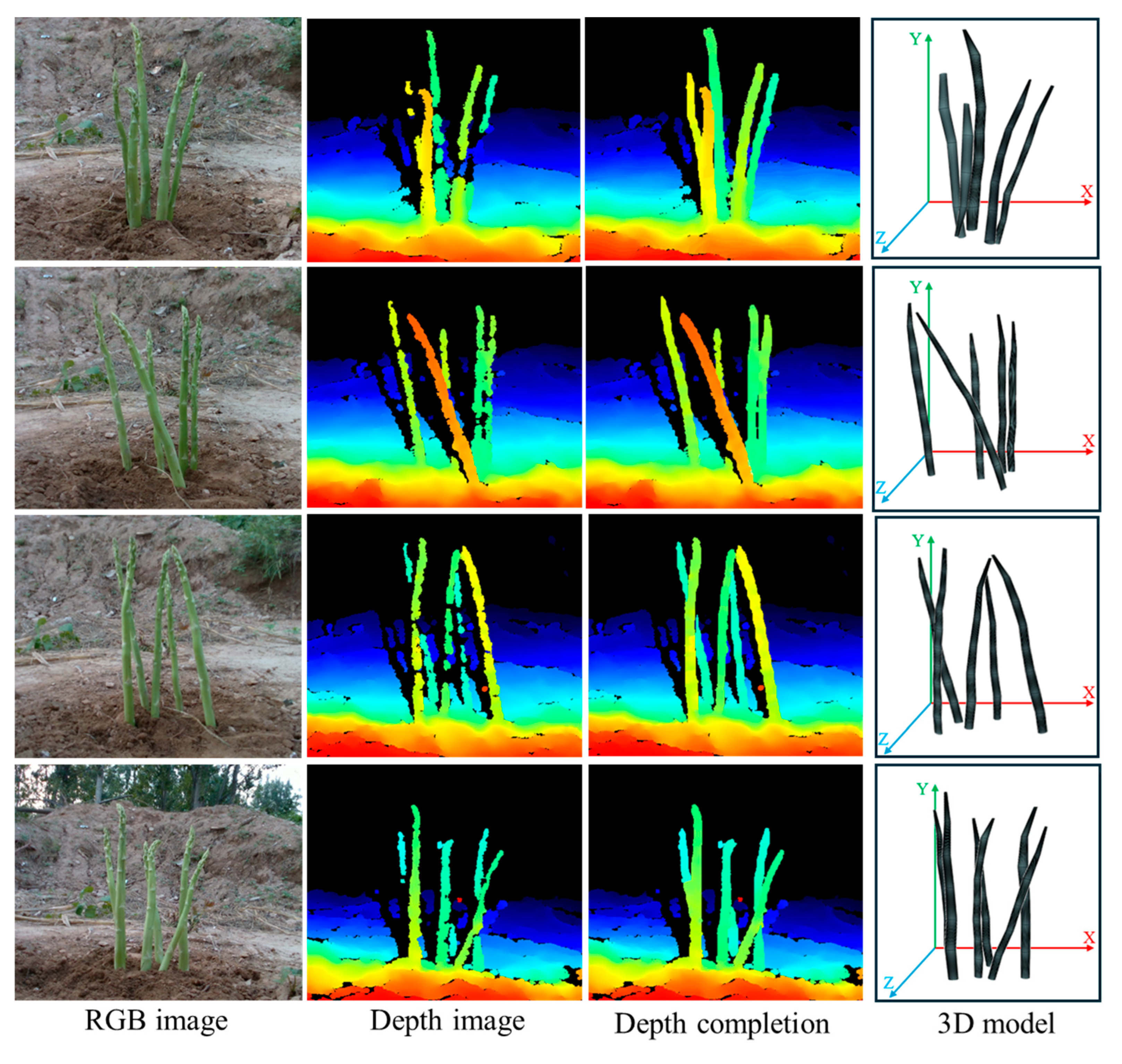
A test was performed to evaluate the visualize the spatial location information of clustered green asparagus in laboratory farm environment. Ten sets of green asparagus images (ranging from 40 to 50 green asparagus) were randomly selected from the sunny and cloudy datasets respectively. And then the actual length of the green asparagus stems and the depth of the distance from the camera were measured based on point cloud. The effects of adaptive-section modeling for some sample asparagus stems (with the bottom occluded, the middle occluded, and the top occluded) are as shown in Figure 21.
To evaluate the length error of green asparagus stems (Lest, cm), it was necessary to know the coordinates (pixels px) of the top point on the stem (utop, utop) and the bottom point on the ground (vbottm, vbottm), as well as the actual length measured on point cloud (Lgt,cm). After these 20 sets of green asparagus images were modeled by YS3AM, we converted the pixel coordinates of the top and bottom points of the stems in model to 3D coordinates under the camera coordinate system, which were the top point (xtop, ytop, ztop) and the bottom point (xbottm, ybottm, zbottm), respectively. Then, based on the research methods in section 2.6, the model-estimated lengths of green asparagus (Lest, the lengths of all detectable green asparagus stem in each image) were compared with the actual lengths measured by point cloud (Lgt), where gt represented the ground truth measurement. The Pearson’s coefficient, R², and Root Mean Square Error (RMSE) were used to compare the differences between the model-estimated stem lengths and the actual lengths.
To further determine the accuracy of the spatial information of green asparagus, the lowest (xbottm, ybottm, zbottm) and highest (xtop, ytop, ztop`) points on the ground of each recognized green asparagus stem were taken to test the depth values with the binocular camera in the Z-axis direction, respectively. Subsequently, the Pearson’s coefficient, R², and RMSE were also used to evaluate the model test results and the actual point cloud measurements.
Figure 21.
Adaptive-Section Modeling of Green Asparagus.
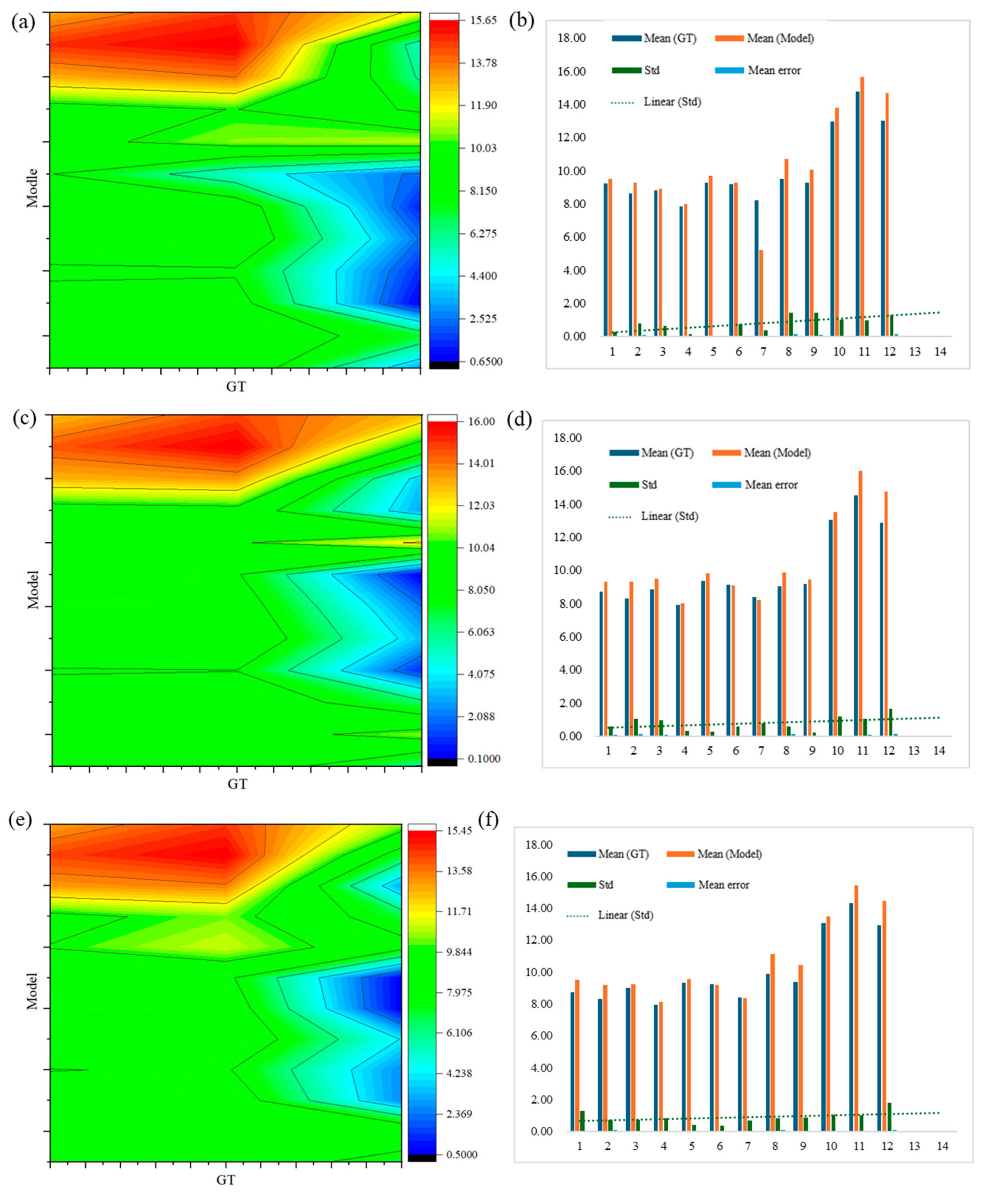
As could be seen from Table 12, in the Sunny dataset, a total of 54 green asparagus were labeled in 10 groups of data, and 40 were detected, with a detection rate of 74.07%. In the Cloudy dataset, a total of 49 green asparagus were labeled in 10 sets of data tested, and 34 green asparagus were detected, with a detection rate of 67.35%. The true-positive detection rate of Sunny environment is 9.98% higher than that of in the Cloudy dataset. The detection effect of Sunny dataset is better than that of Cloudy dataset, which was probably due to the image matching error caused by the change of natural light angle and light intensity. By comparing the spatial visualization results of green asparagus identified under two lighting cases, it was not difficult to find that the depth error of the bottom point in the Sunny dataset was much smaller than that in the Cloudy dataset (0.11cm<0.26cm), and the percentage of error was also much smaller than that in the Cloudy dataset (0.25%<0.68%). Similarly, the depth error of the top point of the stem in the Sunny dataset was smaller than that in the Cloudy dataset (0.90cm<1.87cm), and the percentage error was also much smaller than that in the Cloudy dataset (2.62%<3.22%).
The length results of asparagus stem estimated by the model in both Sunny and Cloudy dataset and the actual value measured in the field are shown in Fig.22. In the Sunny dataset, the R², RMSE and Pearson’s coefficient of the green asparagus stem length were 0.97, 0.71 and 0.99, respectively (Figure 22a). Following a similar pattern in the Cloudy dataset, the R², RMSE, and Pearson’s coefficient were 0.91, 0.77, and 0.91 for green asparagus stem length, respectively (Figure 22b). Overall, both light cases tended to overestimate or underestimate the size of the actual green asparagus, mainly due to light and surrounding background distortion. However, in all cases, the overestimated and underestimated green asparagus lengths compensated for each other, resulting in a slope close to 1:1 between the YS3AM estimated length and the actual measured length (the regression slopes ranging from 0.99 to 1.01).
The depth comparison results of bottom points and top points of the asparagus stem estimated by the model in both datasets with the real value measured in the field is shown in Figure 23. In the Sunny dataset, the R², RMSE, and Pearson’s coefficient of the bottom depth estimation were 0.96, 0.96, and 0.98 respectively (Figure 23a), while the R², RMSE, and Pearson’s coefficient of the top depth estimation were 0.836, 7.44, and 0.915 respectively (Figure 23c). In the Cloudy dataset, the R², RMSE and Pearson’s coefficient of the bottom depth were 0.76, 1.25 and 0.87 respectively (Figure 23b); the R², RMSE and Pearson’s coefficient of the top depth were 0.784, 4.435 and 0.889 respectively (Figure 23d). The slope between estimated bottom depth distance from the camera and the actual measured distance was slightly different in the two lighting environments, with a slope of 0.91 for Sunny dataset and 0.62 for Cloudy dataset. The slope of top point in the two light cases were 0.94 and 0.907 respectively. It was clear that the estimated depth values for the green asparagus all deviated from the actual measurements and were more prominent in the Cloudy dataset. This was because in the Cloudy dataset, the light intensity was not large, the color of the end of the stem was dark, and the color was similar to the land, and the image distortion was serious. As for the depth test of the highest point, due to the gradual thinning of the stem from bottom to top, the discernible area of the sensor in the stem tip became smaller, the gradient of depth information became steeper, and the data mutation was serious. Affected by the accuracy and error of the sensor, the detection error became larger.
Although the detection of clustered green asparagus in Sunny dataset might be the best solution for building 3D models, the effects caused by light and the hardware of sensor could not be completely ignored, even in manual-managed greenhouses. The YS3AM could optimize the detection of clustered green asparagus by obtaining a larger sensing field at different scales and combining the CA-attention mechanism to optimize the detection of outdoor occluded objects. The Cloudy dataset leaded to a decrease in the resolution of some image regions, and the distortion problem might be the main reason for the decrease in the detection accuracy of deep neural networks. In this paper, the detection of clustered green asparagus in the Sunny dataset was slightly better than in the Cloudy dataset. However, for harvesting under outdoor natural light conditions, the results of both methods were satisfactory.
4. Conclusions
To accurate obtain spatial positioning for automatic harvesting robot, this paper develops a novel 3D adaptive-section modeling method, YS3AM, to enhance the precision and efficiency of green asparagus harvesting, filling the gap in previous research. This model achieves precise segmentation of individual asparagus stems in RGB-D images and utilizes a voxel-based modeling approach, combining binary masks and depth maps, to reconstruct 3D models of green asparagus, which offers a viable pathway for real-time 3D modeling in harvesting robot for green asparagus. The conclusion s are as follows:
- (1)
- YS3AM demonstrates stable performance under varying lighting, with improved results on sunny days. Ablation tests shows that YS3AM increased precision by 0.81%, recall by 1.73%, mAP by 1.88%, F1 score by 1.27%, and reduced final loss by 0.032 over YOLOv7.
- (2)
- By segmenting asparagus stems into 4-10 sections based on length, the model meets MAX(RMSEi) requirements, significantly reducing discrepancies between point cloud measurements and model predictions.
- (3)
- Field tests shows that adaptive-section based on asparagus length provided a strong fit, with average RMSE in length (0.74) and bottom depth (1.105) under varied lighting.
- (4)
- YS3AM achieves near real-time detection with an average image processing time of 22 ms, making it suitable for deployment in the Robot Operating System (ROS).
Future work will refine occlusion handling and integrate decision-harvesting into the deep learning model to improve harvesting robustness. Enhancing camera calibration, binocular matching, and lighting stability will also be essential for accurate spatial positioning and consistent performance.
Author Contributions
Si Mu: Writing - original draft, Methodology, Data curation, Validation, Software. Jian Liu: Methodology, Investigation, Data curation, Validation. Ping Zhang: Methodology, Investigation, Validation. Jin Yuan: Writing - Review & Editing, Conceptualization, Funding acquisition, Supervision. Xuemei Liu: Methodology, Investigation, Resources, Project administration.
Data Availability Statement
Data will be made available on request.
Acknowledgments
This work was supported by National Natural Science Foundation of China (52275262) and Cotton Industry Technology System and Industrial Innovation Team Projects in Shandong Province (SDAIT-03-09).
Conflicts of Interest
The authors declare no conflict of interest.
References
- Anasosalu Vasu, P.K., Gabriel, J., Zhu, J., Tuzel, O., Ranjan, A.J.a.e.-p., 2022. MobileOne: An Improved One millisecond Mobile Backbone, p. arXiv:2206.04040.
- Bac, C.W., Henten, E.J.v., Hemming, J., Edan, Y., 2014. Harvesting Robots for High-value Crops: State-of-the-art Review and Challenges Ahead. J. Field Robotics 31, 888-911. [CrossRef]
- Bargoti, S., Underwood, J.J.a.e.-p., 2016. Deep Fruit Detection in Orchards, p. arXiv:1610.03677.
- Bloice, M.D., Stocker, C., Holzinger, A.J.a.e.-p., 2017. Augmentor: An Image Augmentation Library for Machine Learning, p. arXiv:1708.04680.
- Chen, M., Tang, Y., Zou, X., Huang, Z., Zhou, H., Chen, S., 2021. 3D global mapping of large-scale unstructured orchard integrating eye-in-hand stereo vision and SLAM. Computers and Electronics in Agriculture 187, 106237. [CrossRef]
- Clary, C.D., Ball, T., Ward, E., Fuchs, S., Durfey, J.E., Cavalieri, R.P., Folwell, R.J., 2007. Performance and Economic Analysis of a Selective Asparagus Harvester %J Applied Engineering in Agriculture. 23. [CrossRef]
- Dorj, U.-O., Lee, M., Yun, S.-s., 2017. An yield estimation in citrus orchards via fruit detection and counting using image processing. Computers and Electronics in Agriculture 140, 103-112. [CrossRef]
- Dosovitskiy, A., Beyer, L., Kolesnikov, A., Weissenborn, D., Zhai, X., Unterthiner, T., Dehghani, M., Minderer, M., Heigold, G., Gelly, S., Uszkoreit, J., Houlsby, N.J.a.e.-p., 2020. An Image is Worth 16x16 Words: Transformers for Image Recognition at Scale, p. arXiv:2010.11929.
- He, K., Chen, X., Xie, S., Li, Y., Dollár, P., Girshick, R.J.a.e.-p., 2021. Masked Autoencoders Are Scalable Vision Learners, p. arXiv:2111.06377.
- Hong, W., Ma, Z., Ye, B., Yu, G., Tang, T., Zheng, M., 2023. Detection of Green Asparagus in Complex Environments Based on the Improved YOLOv5 Algorithm. 23, 1562. [CrossRef]
- Hou, Q., Zhou, D., Feng, J.J.a.e.-p., 2021. Coordinate Attention for Efficient Mobile Network Design, p. arXiv:2103.02907.
- Hu, K., Chen, Z., Kang, H., Tang, Y., 2024. 3D vision technologies for a self-developed structural external crack damage recognition robot. Automation in Construction 159, 105262. [CrossRef]
- Irie, N., Taguchi, N., Horie, T., Ishimatsu, T., 2009. Asparagus harvesting robot coordinated with 3-D vision sensor, IEEE International Conference on Industrial Technology.
- Kennedy, G., Ila, V., Mahony, R., 2019. A Perception Pipeline for Robotic Harvesting of Green Asparagus. IFAC-PapersOnLine 52, 288-293. [CrossRef]
- Kirillov, A., Mintun, E., Ravi, N., Mao, H., Rolland, C., Gustafson, L., Xiao, T., Whitehead, S., Berg, A.C., Lo, W.-Y., Dollár, P., Girshick, R.J.a.e.-p., 2023. Segment Anything, p. arXiv:2304.02643.
- Kondo, N., Ting, K.C.J.A.I.R., 1998. Robotics for Plant Production. 12, 227-243. [CrossRef]
- Ku, J., Harakeh, A., Waslander, S.L.J.a.e.-p., 2018. In Defense of Classical Image Processing: Fast Depth Completion on the CPU, p. arXiv:1802.00036.
- Lecun, Y., Bottou, L., Bengio, Y., Haffner, P., 1998. Gradient-based learning applied to document recognition. Proceedings of the IEEE 86, 2278-2324. [CrossRef]
- Leu, A., Razavi, M., Langstadtler, L., Ristic-Durrant, D., Raffel, H., Schenck, C., Graser, A., Kuhfuss, B.J.I.A.T.o.M., 2017. Robotic green asparagus selective harvesting. 2401 - 2410. [CrossRef]
- Li, P., Liu, X., Li, Y., Liu, C., 2021. Visual Recognition of Green Asparagus in the Field Based on Dual-Channel Threshold Segmentation and CNN %J Journal of Agricultural Mechanization Research. 43, 19-25.
- Li, S., Zhang, S., Xue, J., Sun, H., 2022. Lightweight target detection for the field flat jujube based on improved YOLOv5. Computers and Electronics in Agriculture 202, 107391. [CrossRef]
- Liu, M., Jia, W., Wang, Z., Niu, Y., Yang, X., Ruan, C., 2022. An accurate detection and segmentation model of obscured green fruits. Computers and Electronics in Agriculture 197, 106984. [CrossRef]
- Mu, S., Dai, N., Yuan, J., Liu, X., Xin, Z., Meng, X., 2024. S2CPL: A novel method of the harvest evaluation and subsoil 3D cutting-Point location for selective harvesting of green asparagus. Computers and Electronics in Agriculture 225, 109316. [CrossRef]
- Peebles, M., Lim, S.H., Duke, M., McGuinness, B., 2019. Investigation of Optimal Network Architecture for Asparagus Spear Detection in Robotic Harvesting. IFAC-PapersOnLine 52, 283-287. [CrossRef]
- Ren, S., He, K., Girshick, R., Sun, J., 2017. Faster R-CNN: Towards Real-Time Object Detection with Region Proposal Networks. IEEE Trans Pattern Anal Mach Intell 39, 1137-1149. [CrossRef]
- Sakai, H., Shiigi, T., Kondo, N., Ogawa, Y., Taguchi, N., 2013. Accurate Position Detecting during Asparagus Spear Harvesting using a Laser Sensor. Engineering in Agriculture, Environment and Food 6, 105-110. [CrossRef]
- Wang, X., Li, W., Wang, L., Shi, Y., Wu, Y., Wang, D., 2023. Method of Detection-Discrimination-Localization for Mature Asparagus Based on Improved YOLACT++ %J Transactions of the Chinese Society for Agricultural Machinery. 54, 259-271.
- Xiang, R., Ying, Y., Jiang, H., 2013. Development of Real-time Recognition and Localization Methods for Fruits and Vegetables in Field %J Transactions of the Chinese Society for Agricultural Machinery. 44, 208-223. [CrossRef]
- Zheng, Y.Y., Kong, J.L., Jin, X.B., Wang, X.Y., Zuo, M., 2019. CropDeep: The Crop Vision Dataset for Deep-Learning-Based Classification and Detection in Precision Agriculture. Sensors (Basel) 19, 1058. [CrossRef]
Figure 1.
Methodology flow chart.
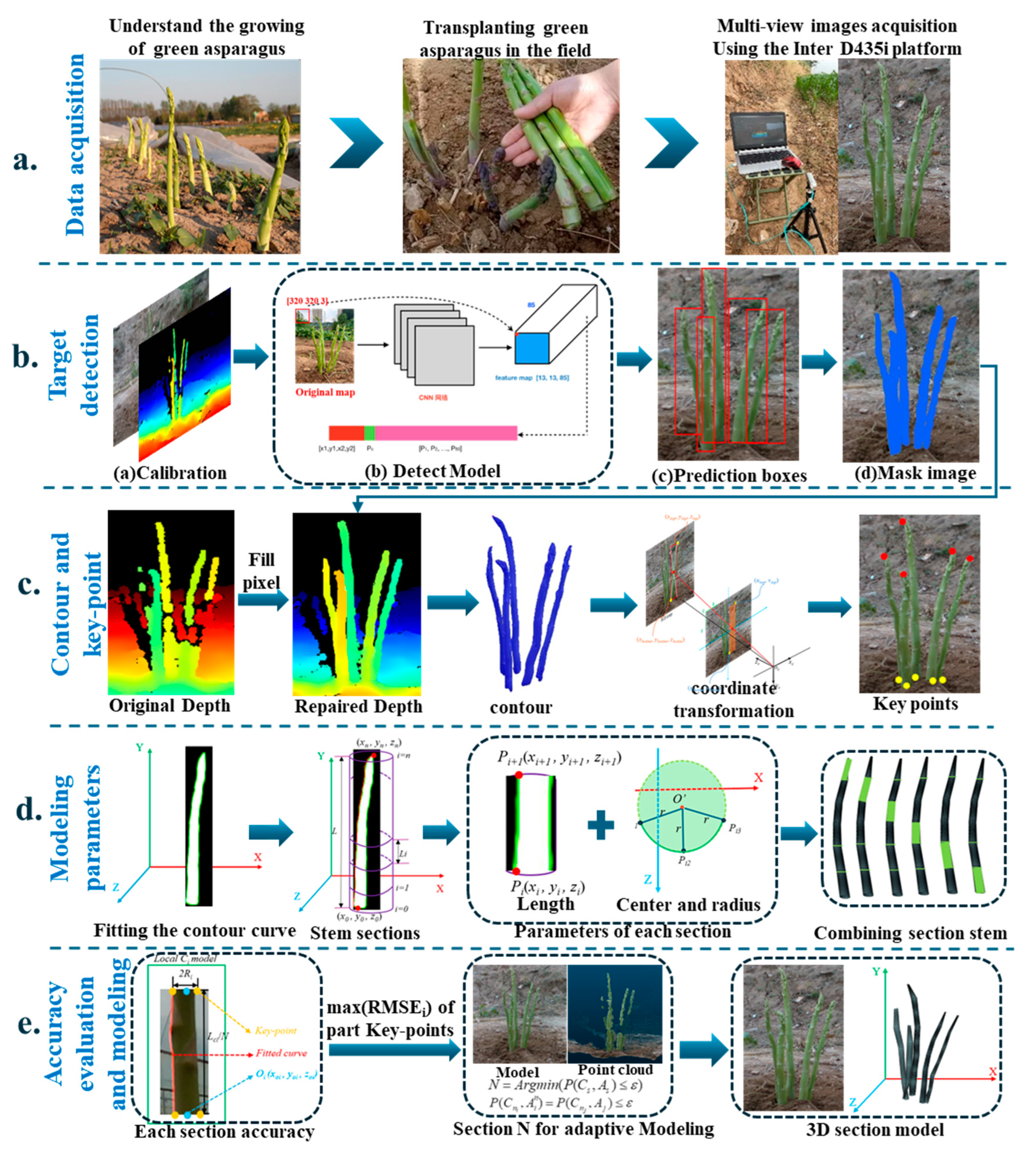
Figure 2.
Green asparagus images collected at different light conditions and at different angles.
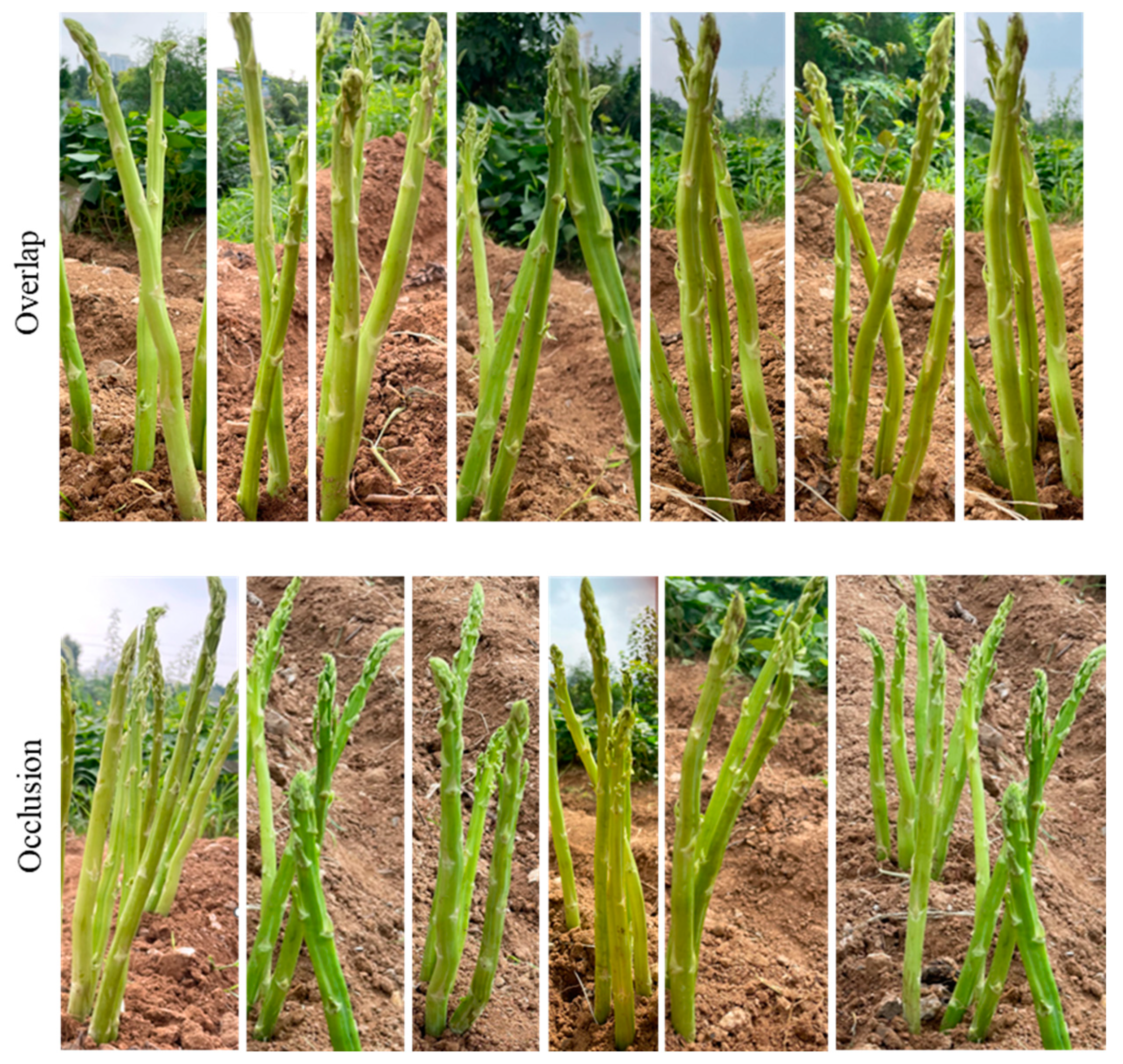
Figure 3.
Some augmentation effects of green asparagus.
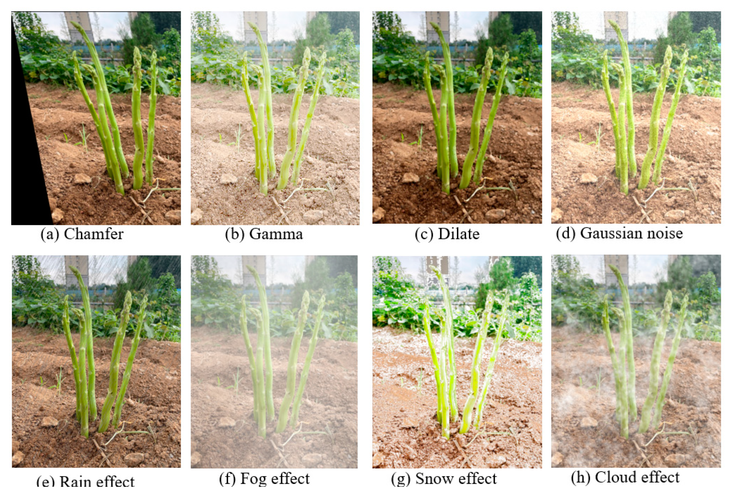
Figure 4.
The building block of MobileOne.
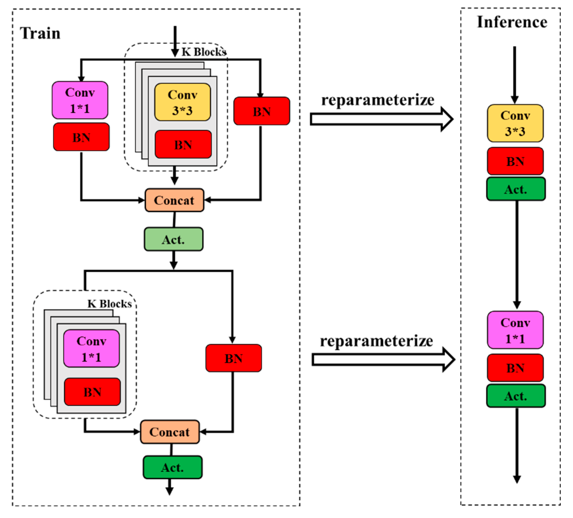
Figure 5.
CAConv. (a) MPConv. (b) Improved CAConv.
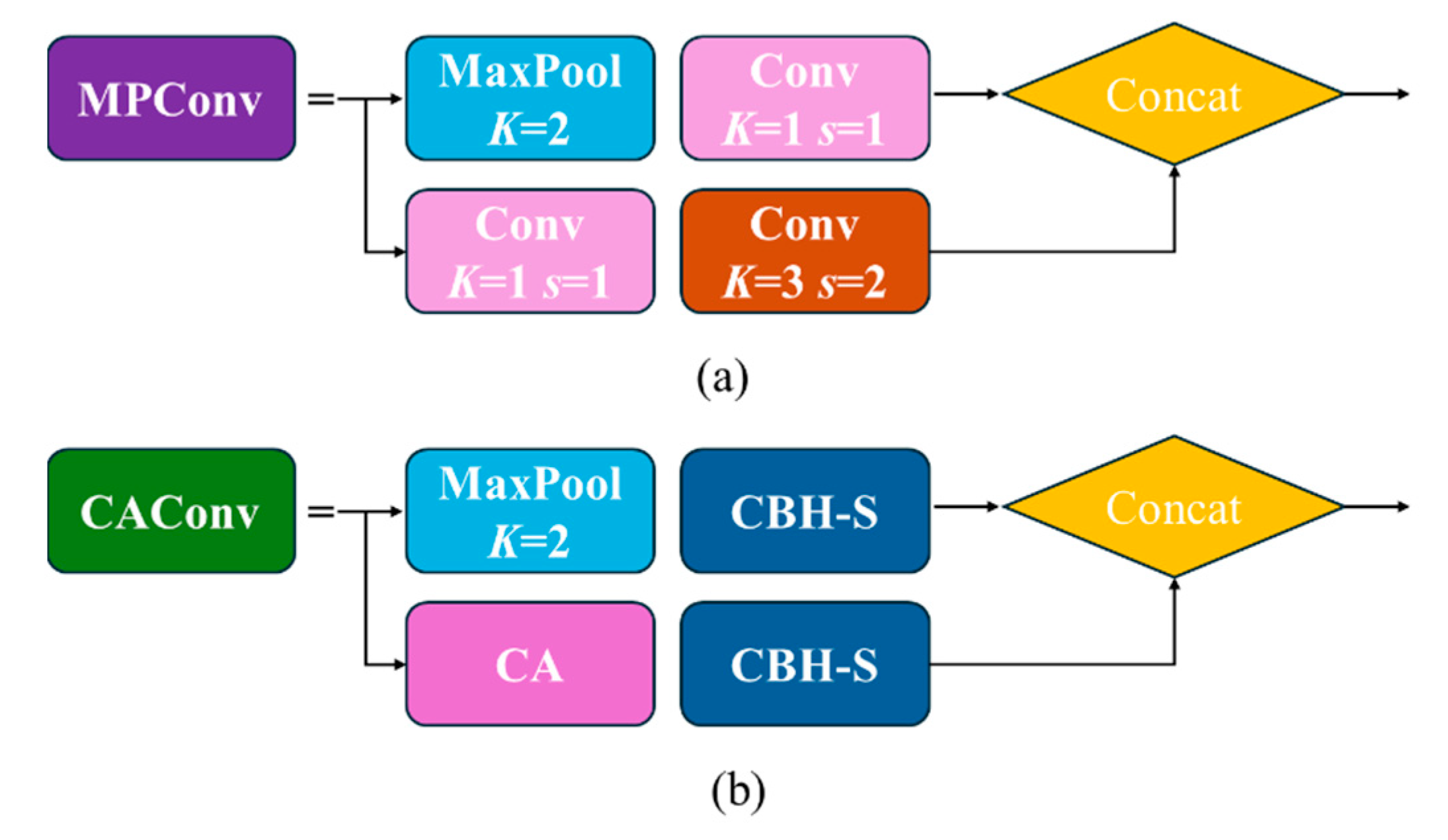
Figure 7.
Recognition and semantic segmentation of green asparagus.
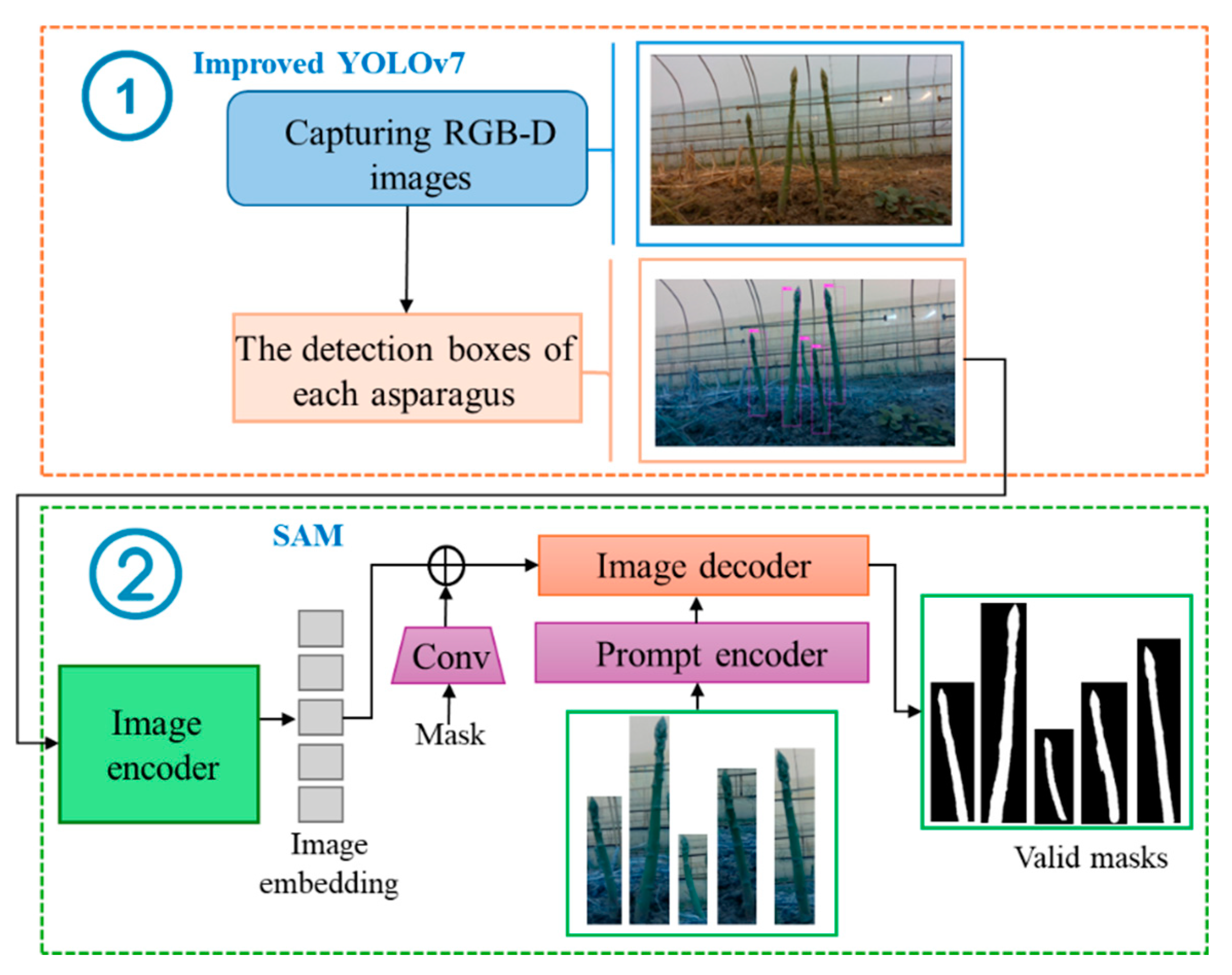
Figure 9.
Coordinate transformation of pixel points of green asparagus stems.
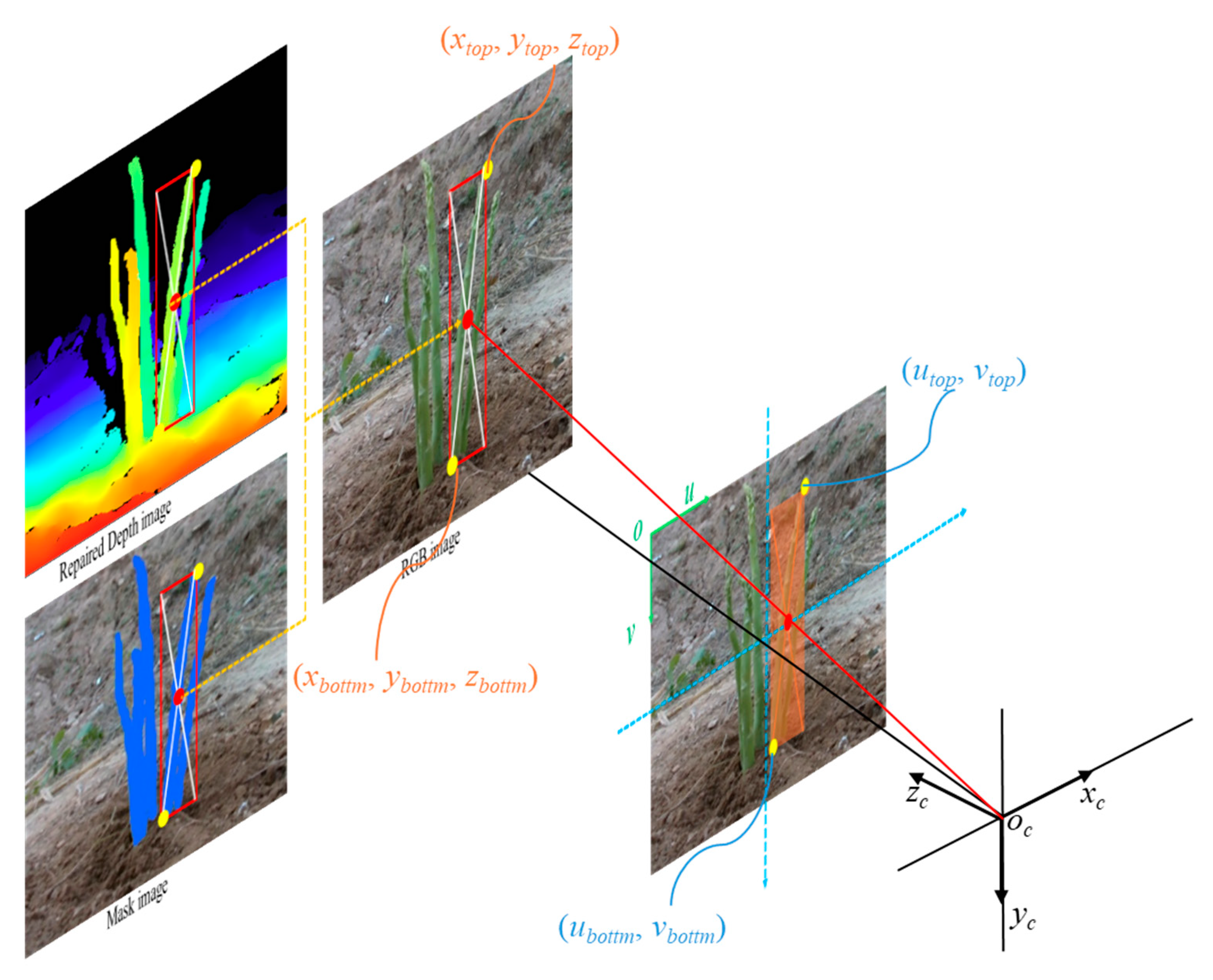
Figure 11.
Calculating the length of each stem using the least square fitting curve.
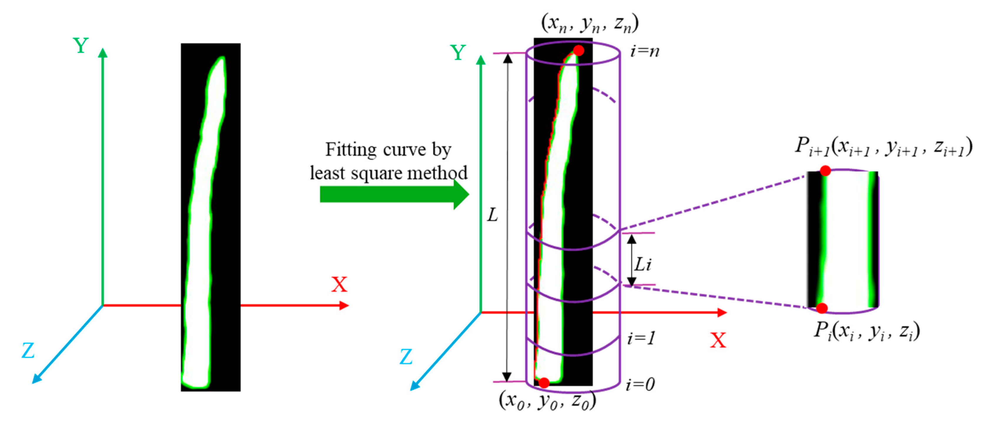
Figure 15.
Results of evaluation indicators for different models.
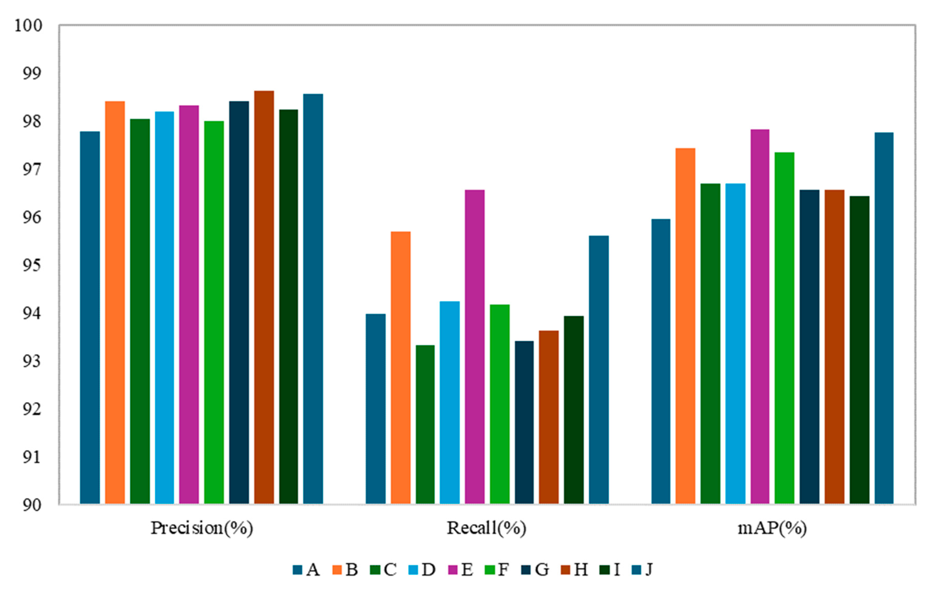
Figure 16.
Targets used for the key-point test. (a) 15~20cm, (b) 21~25cm, (c) 26~30cm, (d) 31~35cm.
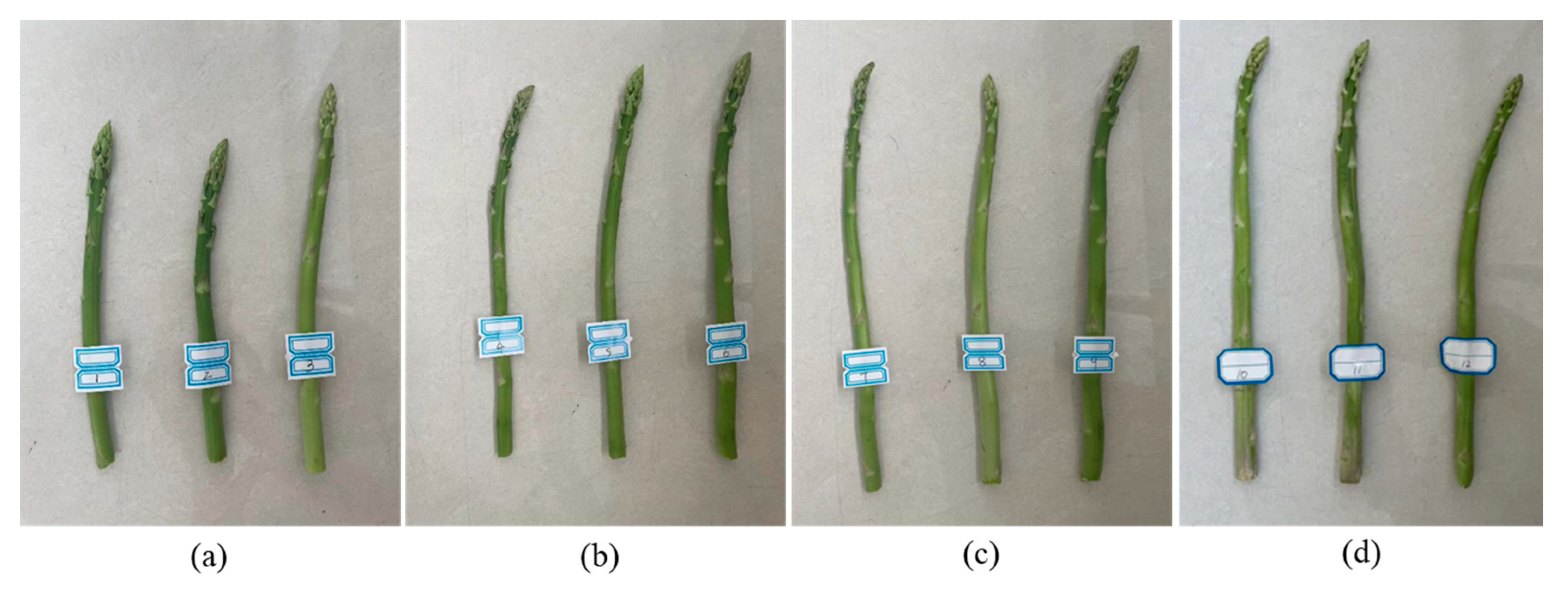
Figure 17.
Key-point test.
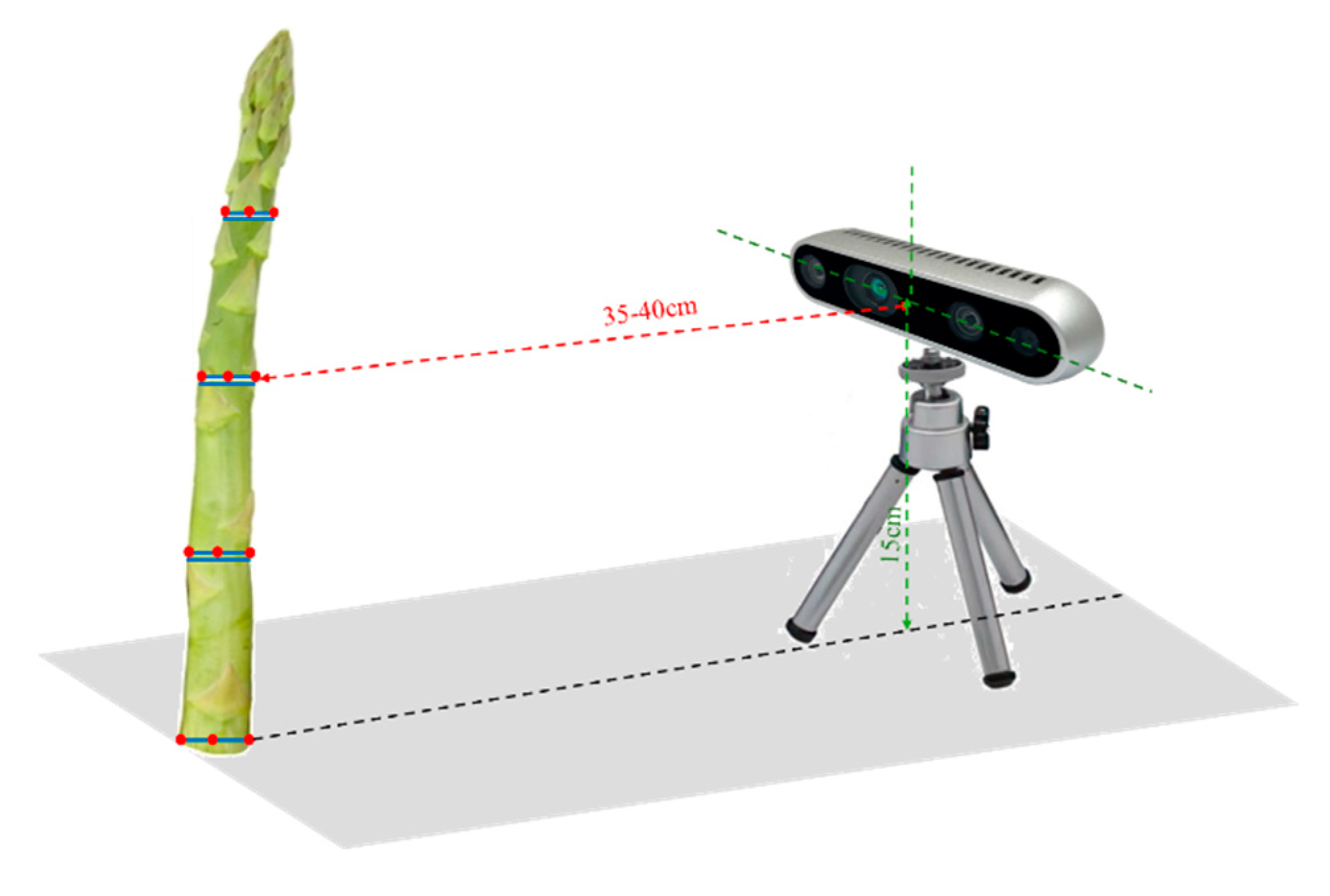
Figure 18.
Examples of different 3D Section Models. .
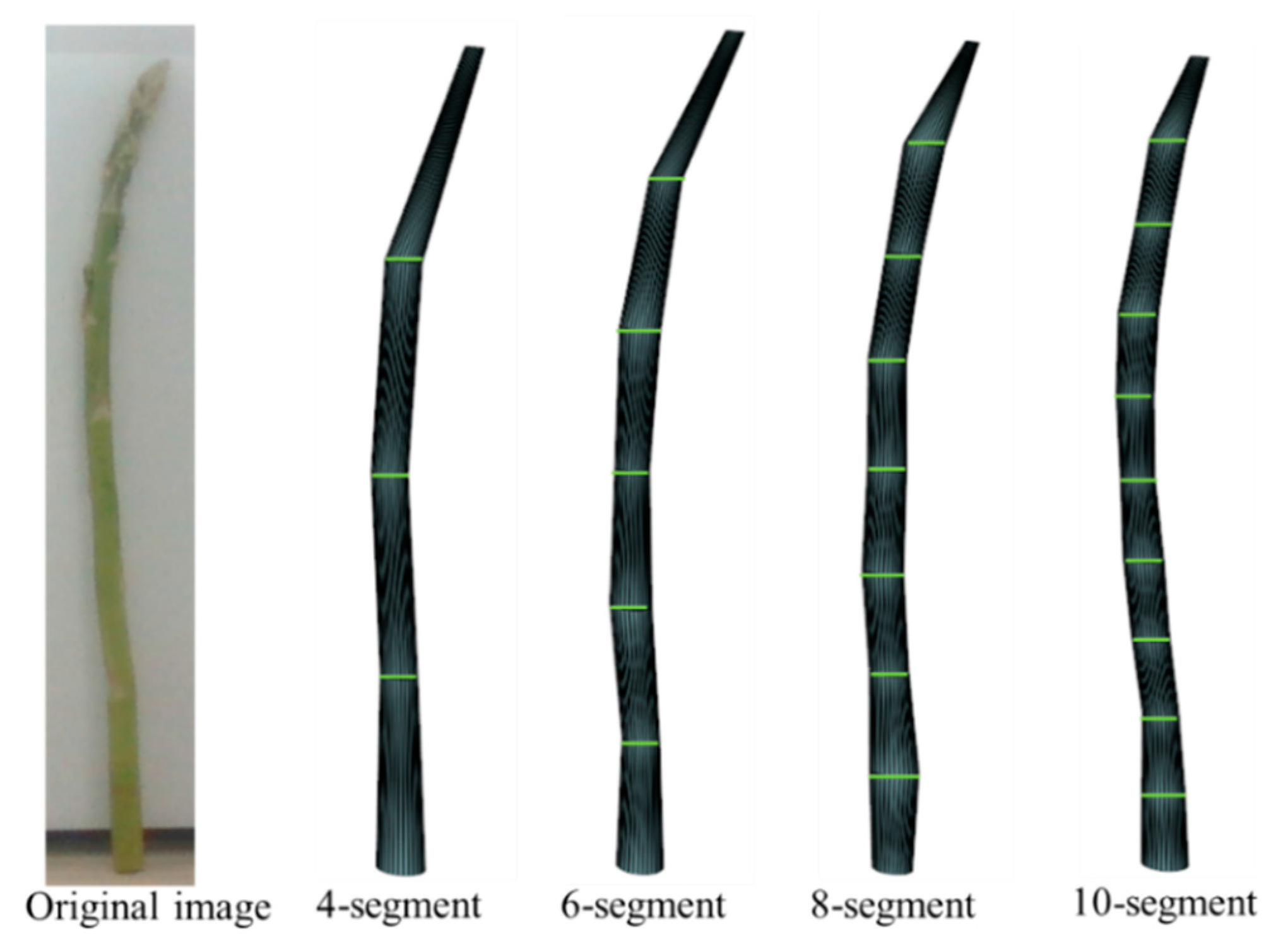
Figure 22.
The YS3AM estimated of green asparagus length (Lest) using (a) Sunny and (b) Cloudy datasets and compared it to the lengths of green asparagus (Lgt) measured manually on the ground. The shaded area indicated the size of the confidence interval for the regression estimates.
Figure 22.
The YS3AM estimated of green asparagus length (Lest) using (a) Sunny and (b) Cloudy datasets and compared it to the lengths of green asparagus (Lgt) measured manually on the ground. The shaded area indicated the size of the confidence interval for the regression estimates.

Figure 23.
YS3AM estimated the ground lowest points of green asparagus stem in (a) Sunny and (b) Cloudy datasets and compared them with the manual measurements. And estimated the highest points of the stem in (c) Sunny and (d) Cloudy datasets, comparing these as well with the manual measurements. The shaded area indicated the size of the confidence interval for the regression estimates.
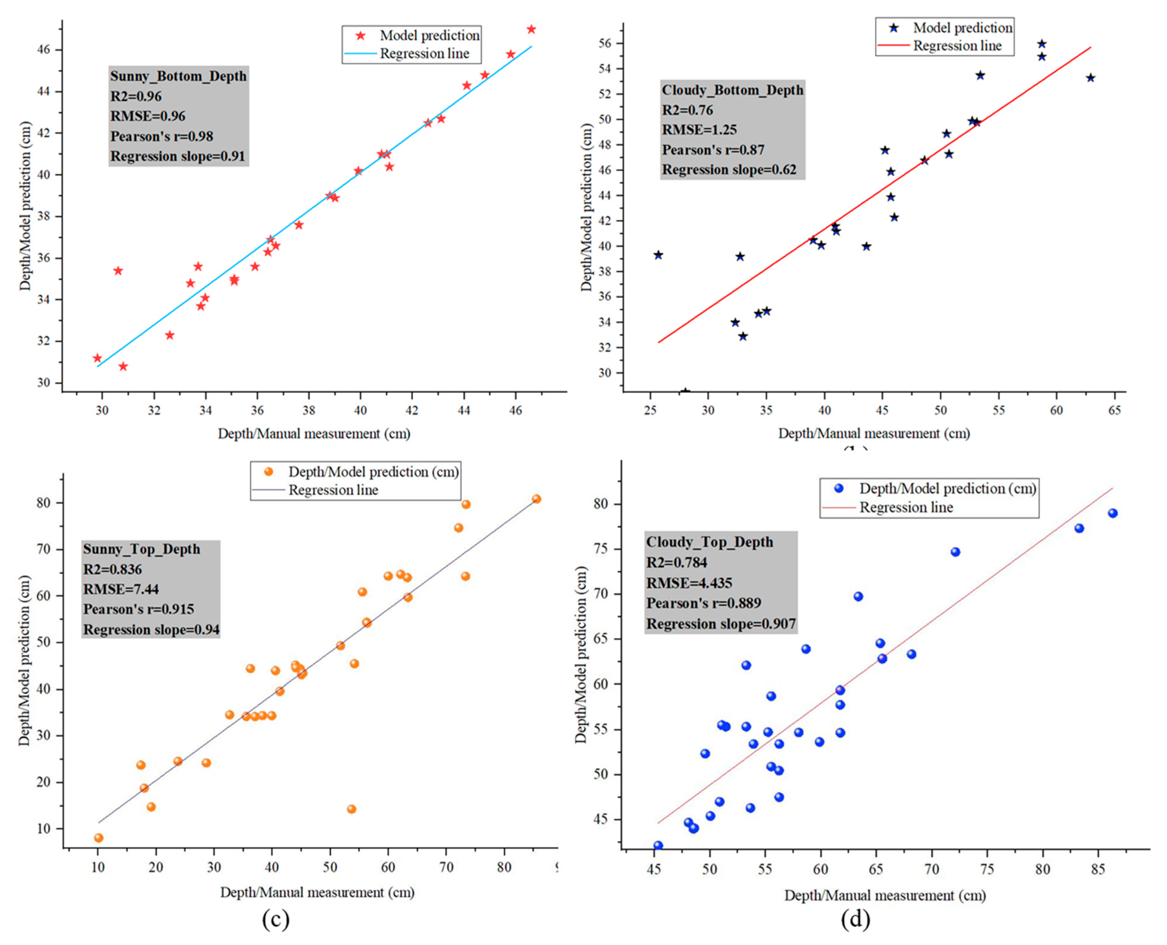
Table 1.
Dataset division.
| Data Set | Training Images/Instances |
Testing Images/Instances |
Total Images/Instances |
|---|---|---|---|
| Sunny | 1746/7888 | 582/2600 | 2328/10488 |
| Cloudy | 1539/6353 | 513/2251 | 2052/8604 |
| Total | 3285/14241 | 1095/4851 | 4380/19092 |
Table 2.
Pseudocode for Pixel Block Completion.
|
RGBimg, Depthimg, Maskimg; Maskimg ← YS3AM(RGBimg); Depth_hsv_img = convert_to_hsv (Depthimg); H_channel, S_channel, V_channel = split_hsv_channels (Depth_hsv_img); Processed_Depthimg = filter_depth_image (V_channel, Depthimg); Max_Iterations, Threshold tempDepthMap ← Processed_Depthimg FOR each pixel (i, j) = =null in Depthimg: IF Maskimg [i][j] = = OBJECT: neighbors = getNeighbors (tempDepthMap, i, j); validDepths = filterValidDepths(neighbors); IF validDepths is not empty: eroded_Maskimg [i][j] = reduce_noise (Maskimg, tempDepthMap [i][j], EROSION_KERNEL_SIZE); dilated_depth_image = fill_missing_pixels (tempDepthMap [i][j], DILATION_KERNEL_SIZE, eroded_Maskimg [i][j]); tempDepthMap [i][j] = average(dilated_depth_image[i][j]); IF maxDifference (tempDepthMap, Depthimg) < Threshold: BREAK; RETURN completedDepthMap; |
Table 3.
Pseudocode for 3D section of stem.
|
RGBimg, Depthimg; Boxes, Maskimg ← YS3AM(RGBimg); for each in Boxes: asp = SeparateAsparagus (each, Maskimg); Top, Bottom, Left, Right = GetKeyPoint(asp); L = Calculate_L (asp, Depthimg); for i in N: BottomPos = LofAsparagus* (i-1) /N+ Bottom; R = Calculate_R (asp, BottomPos, Depthimg); C = GetCenterPoint (asp, BottomPos, Depthimg); x, y, z = MapPostoCamera (C, R, L, Depthimg); PlotCylinder (x, y, z); endfor endfor |
Table 4.
Pseudocode for the computation of accuracy metrics in section modeling of stem.
|
RGBimg, Depthimg; Maskimg ← YS3AM(RGBimg); KeyPoints = []; ModelPoints = []; RMSE_Ci = 0; for pixel in Maskimg, Depthimg: SpecialPoints = findExtremePoints (Maskimg, Depthimg) KeyPoints ← CalculateCenter(SpecialPoints) ModelPoints ← MapModelCenter(SpecialPoints) endfor for Kpoint, Ppoint in KeyPoints, ModelPoints: RMSE_Ci += sqrt ((Kpoint - Ppoint) ^2); Endfor RMSE_Ci = RMSE_Ci/Sizeof (KeyPoints); |
Table 5.
Pseudocode for Calculating the Number of Sections for the Stem Adaptive Modeling.
|
ε = 5×10⁻³; ni = N; RMSE = CalculateP (); while not meet RMSE < ε: if ni > Nmax; ni = N+1; RMSE = CalculateP (); endwhile return ni; |
Table 6.
Hardware configuration and Experimental environment.
| Hardware | Configuration | Environment | Version |
| OS | Windows11 | Python | 3.8 |
| CPU | Intel(R) Core (TM) i9-12900H @2.50GHz | PyTorch | 1.12 |
| GPU | GeForce RTX 3060(6G) | PyCharm | 2022.3.1 |
| RAM | 16G | CUDA | 11.6 |
| HardDisk | 1T | cuDNN | 8.8.0 |
Table 8.
The ablation experiment results.
| Model | CBH-S | MobileOne | CAConv | Cross-scale fusion | Precision (%) |
Recall (%) |
mAP (%) |
Final loss | F1 (%) |
Detection time per image (ms) |
GFLOPs |
| A | 97.79 | 93.98 | 95.96 | 0.062 | 95.85 | 14.9 | 105.1 | ||||
| B | ★ | 98.42 | 95.69 | 97.45 | 0.031 | 97.04 | 13.2 | 103.2 | |||
| C | ★ | 98.05 | 93.34 | 96.71 | 0.059 | 95.64 | 16 | 43 | |||
| D | ★ | 98.19 | 94.25 | 96.71 | 0.059 | 96.18 | 14.7 | 55.1 | |||
| E | ★ | 98.32 | 95.68 | 97.82 | 0.030 | 96.98 | 95.6 | 104.8 | |||
| F | ★ | ★ | 98.00 | 94.19 | 97.36 | 0.061 | 96.06 | 14.9 | 47.9 | ||
| G | ★ | ★ | ★ | 98.41 | 93.42 | 96.56 | 0.061 | 95.85 | 14.1 | 50.7 | |
| H | ★ | ★ | ★ | 98.64 | 93.64 | 96.58 | 0.060 | 96.07 | 12.8 | 42.9 | |
| I | ★ | ★ | ★ | 98.25 | 93.95 | 96.43 | 0.059 | 96.05 | 13 | 53 | |
| J | ★ | ★ | ★ | ★ | 98.58 | 95.61 | 97.76 | 0.030 | 97.07 | 12 | 50.8 |
Table 9.
The RMSE result of key point location deviation.
| 4-section | 6-section | 8-section | 10-section | ||
| Group 1 | 1 | 0.00307 | 0.00299 | 0.0028 | 0.00206 |
| 2 | 0.00481 | 0.00461 | 0.00171 | 0.00296 | |
| 3 | 0.00468 | 0.00611 | 0.00662 | 0.00621 | |
| Group 2 | 4 | 0.00258 | 0.00301 | 0.00279 | 0.00288 |
| 5 | 0.00523 | 0.00389 | 0.00299 | 0.00303 | |
| 6 | 0.000763 | 0.00444 | 0.00659 | 0.00374 | |
| Group 3 | 7 | 0.00354 | 0.00281 | 0.00419 | 0.00274 |
| 8 | 0.01299 | 0.01358 | 0.00261 | 0.00177 | |
| 9 | 0.01646 | 0.05857 | 0.01982 | 0.00322 | |
| Group 4 | 10 | 0.01053 | 0.00751 | 0.01128 | 0.00347 |
| 11 | 0.00318 | 0.00392 | 0.00216 | 0.00397 | |
| 12 | 0.00248 | 0.00293 | 0.00252 | 0.00313 |
Table 12.
Comparison of asparagus detection results with two different datasets.
| Imaging method | Label asparagus count | True positive (correctly detected) | Length error (cm) |
Length error (%) | Bottom depth error (cm) | Bottom depth error (%) | Top depth error (cm) | Top depth error (%) | |
| Asparagus number | Accuracy (%) | ||||||||
| Sunny | 54 | 40 | 74.07 | 0.55 | 2.07 | 0.11 | 0.25 | 0.90 | 2.62 |
| Cloudy | 49 | 34 | 67.35 | 0.63 | 2.84 | 0.26 | 0.68 | 1.87 | 3.22 |
Disclaimer/Publisher’s Note: The statements, opinions and data contained in all publications are solely those of the individual author(s) and contributor(s) and not of MDPI and/or the editor(s). MDPI and/or the editor(s) disclaim responsibility for any injury to people or property resulting from any ideas, methods, instructions or products referred to in the content. |
© 2025 by the authors. Licensee MDPI, Basel, Switzerland. This article is an open access article distributed under the terms and conditions of the Creative Commons Attribution (CC BY) license (http://creativecommons.org/licenses/by/4.0/).
Copyright: This open access article is published under a Creative Commons CC BY 4.0 license, which permit the free download, distribution, and reuse, provided that the author and preprint are cited in any reuse.


