
Submitted:
03 January 2025
Posted:
06 January 2025
You are already at the latest version
Abstract
In arid and semi-arid regions, irrigation is extremely important for agricultural production. However, water salinity is a major threat both to the soil-plant combination and to the longevity of the materials that make up the irrigation system. Drip irrigation with direct and intermittent photovoltaic pumping can play a key role in optimizing irrigation with saline water. This article compares two pump models to understand which has the greatest capacity to reduce the risks of salinity in irrigated agriculture. The evaluation of the ideal pump was conducted using electrical and hydraulic parameters of the motor pump and quality parameters of the water applied by irrigation. The results indicate that the diaphragm pump is more sensitive to disturbances in irrigation management but makes the irrigation system with saline water more resistant to clogging.

Keywords:
solar energy
; chemical clogging
; brackish water
; positive displacement pump
; dynamic pumps
1. Introduction
In arid and semi-arid regions, irrigation is extremely important for agricultural production. However, water salinity is a major threat to both the soil-plant combination and the longevity of the materials that make up the irrigation system.
The salts come with the irrigation water and are accumulated and concentrated in the soil as the water evaporates. To ensure that salinity levels in the soil are not harmful to crop growth, the water applied must be sufficient to meet the plants’ needs and leach the salts from the root zone (Rhoades 1974; Burt and Isbell 2005). However, the implementation of this approach is limited on several occasions, such as when the water table in the area is shallow (Tanji 1990).
Drip irrigation, with its low flow rate and the possibility of frequent applications, makes it possible to maintain high soil moisture in the root zone without the need for leaching (Kang et al. 2010). The pattern of soil salinity depends on soil properties, water and fertilizer management and irrigation design. Several studies have investigated the effects of irrigation parameters with saline water.
Nightingale et al. (1991) concluded that increasing the amount of irrigation reduced salinity in the soil depth below the drip line. Experiments conducted by Khan et al. (1996) indicated that the concentration of solutes in the soil increased with the input concentration, the volume applied and the application rate. Meerbach et al. (2000) showed that salt accumulation in the root zone of cotton changes with the change in irrigation scheme. Souza et al. (2009) demonstrated the advantage of applying small amounts of solution at more frequent intervals to reduce losses through deep percolation of water and solutes. Guan et al. (2013) showed that the low uniformity of irrigation application leads to a large fluctuation in the salt content of the soil layers at a depth of 60 cm.
As well as being useful in developing the design, operation and management of drip irrigation systems with saline water, the results mentioned above are a guide to the development of new technologies and processes that can be applied to irrigation with saline water, such as drip irrigation with direct and intermittent photovoltaic pumping, the focus of this article.
Solar pumping projects first appeared in the late 1970s with applications aimed at supplying water to remote rural communities (CHANDEL et al. 2015). Its use has spread around the world, mainly in developed countries, and it currently has a reliable and consolidated technology with more than four decades of accumulated experience.
Several photovoltaic pumping projects have already been developed and tested (MOECHTAR et al., 1991). These systems work with alternating or direct current, with voltage variation, connected directly or with batteries, using different types of pumps and, above all, operating in different climatic conditions. Kumar et al. (2015) proposed a gravity-fed drip irrigation system integrated with a low-cost solar pumping system. Pande et al. (2003) recommended a project size based on the uniformity of an application. Reça et al. (2016) and Zavala et al. (2020) investigated the multisectoral application of this irrigation model. Ceryera-Gasco et. al. (2020) set out to develop mathematical models to design drip irrigation systems conditioned to this energization system.
In particular, the direct and intermittent application of photovoltaic pumping, i.e. without the use of batteries or water storage tanks, and with the aid of a timer to apply the blade in pulses, it is worth noting that the opportunity to operate the system throughout the morning and part of the afternoon means that irrigation benefits from a long operating time and fluctuating pressure because of fluctuating irradiance. According to Quiang Li (2019), the effect of drip irrigation with a longer floating pressure period was better in reducing clogging by chemical precipitates. Calcium and magnesium precipitates, for example, are mainly formed when the system stops working, in the wet and dry alternation of long-term drip irrigation, the adhesion layer of the chemical deposit on the inner wall of the flow channel gradually thickens, and the adhesive force of the wall increases and causes the capacity of the flow channel emitter to gradually decrease (Liu et al., 2017).
In terms of technology, photovoltaic water pumping systems have made significant advances in the last decade. According to Protoger & Pearce (2000) there are two photovoltaic pumping technologies: the first uses centrifugal (dynamic) pumps, with hydraulic efficiency ranging from 25 to 35%, and low efficiency in situations of low solar radiation. The second technology uses positive displacement pumps (diaphragm pumps), characterized by lower power requirements, high hydraulic efficiency, which can reach up to 70%, but the flow rate is directly proportional to the amplitude of the applied voltage.
In addition, photovoltaic solar pumping projects make use of electronic converters and controllers capable of optimizing the system’s efficiency. By operating directly coupled to the photovoltaic panel, the pump can work in overload at times of high irradiance, and low power when the irradiance is low. Thus, according to Chandel et al. (2015), the use of electronic systems that can optimize the power delivered to the pump available at each moment of operation in the day results in better system performance. Centrifugal pumps, for example, have the load characteristic of being very close to the point of maximum photovoltaic power, making them operate well in this connection model. Positive displacement pumps, on the other hand, have different speed-torque characteristics and are not suitable for direct connection to photovoltaic panels. When these pumps are used, it is advisable to use a power conditioning unit and a power point tracking system.
Against this background, this work is divided into two stages. Firstly, the aim is to find out about the performance of a bench drip irrigation system with direct and autonomous photovoltaic pumping, operating under two pumps with similar powers and different technologies. And finally, to ascertain the quality of irrigation using the most suitable pump for application with saline water in a pulsed pumping system.
2. Materials and Methods
2.1. Site Characterization
The experiment took place from October 2023 to November 2024 in two different locations. The first stage was carried out at the Irrigation and Fertigation Laboratory of the State University of Western Paraná (UNIOESTE), in Cascavel, Paraná, Brazil, geographical coordinates 24° 58’ 0’‘ South and 53° 31’ 48’‘ West. And the last stage was carried out at the training center of the Agricultural Research and Rural Extension Company of Santa Catarina (EPAGRI), in Florianópolis, Santa Catarina, Brazil, geographical coordinates 27° 34’ 54’‘ South and 48° 30’ 22’‘ West.
2.2. Irrigation System
The dripper model used was Netafim’s Aries 16200, with emitters spaced 0.40 m apart and an average flow rate of 1.5 L at 1 bar. The emitter has an internal diameter of 15.5 mm, a thickness of 0.5 mm, a maximum working pressure of 2.5 bar, a filter area of 53 mm², a discharge coefficient of 0.52 and a discharge exponent of 0.46, resulting in a characteristic flow-pressure equation represented by potential equation 01.
where q is the flow rate of the emitter (L.); h is the hydraulic pressure at the water inlet to the emitter (KPa).
A Rain Bird 200 mesh disk filter, a vertical 2.5 bar stainless steel pressure gauge with glycerine and a RainPoint digital flow meter were installed. The measuring range and accuracy of the flow and pressure sensors are shown in Table 1.
To test the irrigation, the system was powered by solar energy with a Resun Solar RS6E 150P module. Precautions were taken to keep the panel clean and avoid external influences. The specifications of the photovoltaic panels are detailed in Table 2.
Energy production data was collected with an M430 DSN VC288 DC 0100 V 10A dual digital voltmeter. Radiation levels were recorded with a portable solar energy meter model SM206. The measuring range and accuracy of the irradiance, voltage and current sensors are shown in Table 1.
This research used two Seaflo motor pumps, the first model SFSP-G500-02A, a centrifugal pump, with a flow rate of 31 L/min, height of 7m, voltage of 12v, nominal current of 4.5A and maximum current of 7.5A. The second model SFDP1-010-035-21, a diaphragm pump, with a flow rate of 3.8 L/min, voltage of 12v, nominal current of 1.6A, maximum current of 2.5A, height of 28m.
The converter under study is an XL4016 voltage regulator (12A, 100W) that converts an input voltage of 8V to 40V to provide a stable output voltage of 1.25V to 36V. It uses the XL4016 switching regulator chip.
The first stage of the project was carried out with the irrigation system installed on a test bench (Figure 1). This bench is 5.0 m long, with four lateral lines spaced 0.5 m apart, where the lateral line can be turned by means of pulleys, making it 10.0 m long. It also has a gutter to return the water to a 200-liter reservoir. The last stage was carried out with an irrigation system installed in the field, under the open sky, with the same dimensions as the first stage.
2.3. Experimental Design
The experimental project was carried out in two stages. Firstly, in order to evaluate the system’s power, efficiency, current and voltage, a 2x2x2 factorial scheme was proposed, in which the first factor consisted of two hydraulic designs: one was connected to an irrigation system consisting of four 10-meter lateral lines, a filter and 30 meters from the main line, and the other was disconnected from the lateral lines of the same irrigation system; the second factor was the absence and presence of the DC converter and the third factor was the type of pump, varying between a centrifugal pump and a diaphragm pump. In this first stage, 25 samples were taken in four irradiance ranges (0 to 300 W.301 to 600 W.601 to 900 W.901 to 1200 W.).
In the second stage, 25 samples were taken to determine the uniformity of the irrigation blade applied under irradiation from 0 to 300 W. with the treatments without the DC converter. Finally, these same 25 uniformity tests, under irradiation from 0 to 300 W. , were carried out with the treatments involving the diaphragm pump with the presence of the DC converter, and the centrifugal pump without the presence of the DC converter, both with intermittent application with 5-minute pulses and saline water.
The saline water came from mixing fertilizers in drinking water. The dilutions were urea at 5 g. and calcium nitrate, magnesium sulphate, potassium chloride, sodium nitrate and iron sulphide, all at a concentration of 1.2 g.. The physicochemical analysis of the saline water used was carried out following the APHA methodology (2012), by the analysis laboratory (LABCAL) and the Integrated Environmental Laboratory (LIMA), both based at the State University of Santa Catarina (UFSC). The parameters are described in Table 3.
It is worth adding that before carrying out the 25 uniformity tests with saline water, the irrigation system was fed with the same water for two months, also in a pulsed manner, twice a week. To do this, 200 liters of saline water were separated in a reservoir and applied until the reservoir was completely empty. The pulsed regime was carried out manually using a stopwatch, alternating between 5 minutes on and 10 minutes off.
2.4. Experimental Procedure
Table 4 shows the equations used to calculate the performance factors used in this study. These are: solar energy (Eq. 02), electrical energy from the panel-pump assembly (Eq. 03), hydraulic energy (Eq. 04), motor assembly efficiency (Eq. 05) and total system efficiency (Eq. 06).
The flow versus head curve for the proposed photovoltaic pumping system was also created under irradiance rates above 1000 W. To do this, the methodology proposed by Cossich et al (2024b) was used to know the flow rate and pressure at the pump outlet under different manometric heights and compare them with the reference heights provided by the manufacturer. 10 repetitions were carried out at 7 different heights with the plate facing north and inclined at 15°, always between 11:30 and 12:30 on clear, sunny days.
To calculate the application uniformity of the irrigation system, data was collected following the methodology of Keller and Karmeli (1974). This approach involves measuring the flow in four drippers per lateral line, including the first dripper, those located 1/3 and 2/3 along the line and the last dripper in four lines. The flow of the drippers was accurately measured using the gravimetric method, collecting volume from the emitters for 5 minutes. The samples were weighed on a digital scale, accurate to 0.1g, and the volumes calculated based on the density of water (1000 kg).
The ISO standard (2006) was used for the hydraulic evaluations. The average flow rate was calculated according to Equation 07.
where q is the Dripper flow rate, L.; V is the collected volume, mL; and t is the collection time, minutes.
The distribution uniformity coefficient (DUC) proposed by (Merrian & Keller 1978) was used, as shown in Equation 08.
where DUC is the distribution uniformity coefficient, in %; is the average of the lowest quartile of the volumes of water contained in the collectors, in mm; and is the overall average of the values of the volumes of water collected, in mm.
The division developed by Keller and Bliesner (1990), shown in Table 5, was adopted to classify the efficiency of the irrigation system.
The methodology of Montgomery (2016) was used to interpret Shewhart and EWMA control charts of the DUC values.
According to the Shewhart control chart, the number of observations in the sample is n = 1, consisting of a single individual unit. Control charts are used for individual measurements, based on the moving interval of two consecutive observations as an estimate of process variability, calculated by MR = |xi - xi-1|, where i is the observed point (Montgomery, 2016). The upper and lower control limits were calculated by Equations 09 and 10, respectively (Montgomery 2016).
In the Shewhart control charts, the control limits are calculated considering L = 3, which means that 370 samples are needed to indicate an out-of-control condition, and that 99.73% of the samples will be within the control limits. With L = 2 and only 25 samples, 95.45% of the samples will be within the control limits, indicating an out-of-control condition after 22 samples taken. These values are based on common causes acting in the system and a normal distribution, according to Montgomery (2016).
The EWMA control chart is ideal for dealing with the accumulation of successive data, giving more weight to recent data. It produces a weighted average of all past and current observations and is more robust than the Shewhart chart to non-normality of data. It is defined as follows:
In which: 0 < λ ≤ 1; (target value or average value in control xi). The variance of the Z variable is expressed as Equation 12.
where σ is the standard deviation of the data in relation to the mean, λ is the weight assigned to each sample, and i is the order of the sample used.
The UCL and LCL of the EWMA control table can be calculated by Equations 13 and 14, respectively.
where is the mean of the data; λ is the weight assigned to each sample, which varies from 0 to 1; L is the number of standard deviations used to control the mean to be detected; and i is the order of the sample used. The sample weight constant is 0.25 and the limit amplitude factor λ is L = 2, chosen as in the Shewhart control chart.
In general, values of 0.05 ≤ λ ≤ 0.25 perform well, with λ = 0.05, 0.10 and 0.20 being the most popular. Lower values of λ detect smaller changes, while λ = 1 turns the EWMA into a Shewhart chart (Crowder 1989).
Finally, it is important to note that the normality of the data was checked to determine the statistical comparison tests to be used. The Anderson Darling normality tests were carried out. Subsequently, in the event of non-normality, the Kruskal-Wallis test was applied, followed by the Mann-Whitney multiple comparison test, both with a significance level of 5%. The graphs were calculated using MINITAB software, version 16.
3. Results and Discussion
Figure 2 shows the graphs of the electrical power supplied to the motor pump in relation to the momentary irradiance for the two pump models operating without the aid of controllers and disconnected from the irrigation. It should be noted that the two pumps stabilize in a power range (50W for the centrifugal pump and 24W for the diaphragm pump), even with the increase in irradiance. However, the first difference between the two pumps is the equivalent circuit formed in conjunction with the photovoltaic panel. Due to the difference between the equivalent resistance, the current and voltage supplied to the motor pumps are different to the point where the centrifugal pump reaches a maximum of 52.6W and the diaphragm pump 25.2W.
Vick et. al. (2011) investigated similar curve patterns when investigating the SHURflo Model 9325, Sun Pumps Model SDS-D-228, Robison Model BL40Q and Sun Pumps Model SDS-Q-128 diaphragm pumps in photovoltaic solar pumping.
The choice of a motor pump for application connected directly to the photovoltaic panel is not made by comparing the electrical power supplied to the pump, since they differ in structure and operating mechanisms and do not directly reflect their hydraulic efficiency. However, it can be seen in Figure 2 that the diaphragm pump approaches its maximum electrical power values at lower radiation rates (200W. ) compared to the diaphragm pump (580W. )).
This characteristic of the electrical power reaching its maximum early favors the diaphragm pump for applications in irrigation with saline water, since operating with lower irradiations makes the system stay on for more hours of the day. According to Liu et al. (2017) calcium and magnesium precipitates, for example, are formed mainly when the system stops operating, in the wet and dry alternation of long-term drip irrigation, the adhesion layer of the chemical deposit on the inner wall of the flow channel gradually thickens, and the adhesive force of the wall increases and causes the capacity of the flow channel emitter to gradually decrease.
Since all the treatments showed similar curves of power supplied versus irradiance, Figure 3 shows the maximum electrical power values achieved for each treatment. According to the graph, the power of the pump operating at zero head is 54W for the centrifugal pump and 48W for the diaphragm pump, according to the manufacturer’s information. With photovoltaic pumping, the centrifugal pump obtained power with a variation of less than 10% in relation to the manufacturer, even with the increase in pressure drop, and the diaphragm pump reduced between 34 and 64%, also in relation to the manufacturer’s characteristics.
Still in relation to Figure 3, the use of the inverter increased electrical power by around 10% when using the centrifugal pump, and with the diaphragm pump there was a decrease of between 40 and 56%. Finally, it should be noted that only with the diaphragm pump did the electrical power change when connected to the lateral irrigation lines, with an increase of between 24 and 37%.
Studying a centrifugal pump, Mokeddem et al. (2011) found similar results when investigating a photovoltaic water pumping system at a fixed height of 11m. With a 750W pump, the electrical power supplied reached around 850W, i.e. 13% more than the nominal electrical power.
In relation to diaphragm pumps, Vick et al. (2011) found a drop of approximately 54% when using a 150W pump at a height of 20m, with the power supplied stabilizing at approximately 70W.
This sensitivity in the electrical power present in the diaphragm pump as a function of the addition of the converter or loss of load, here specifically the irrigation system, highlights the importance of preventive maintenance in the case of its use in irrigation with saline water. Corrosion of internal parts, as well as clogging of the irrigation system, can increase the power of the motor pump, causing it to break down long before the useful life calculated by the manufacturer. Vick et al. (2011) point out that one diaphragm pump manufacturer recommends that after one or two years the pumps should be retrofitted with new parts.
Table 6 shows the behavior of the flow rate and pressure on the pipe wall at the motor pump outlet, according to the manufacturer, as well as when the pump operates autonomously with the photovoltaic system. The photovoltaic system proposed in this project reduced the flow rate of the centrifugal pump, for example, to zero head, this reduction was 50%. With the diaphragm pump, the flow rate increased by around 20%.
According to Cossich et. al (2024b) the pressure values measured with a manometer on the pipe wall near the pump outlet are not equal to the total height of the system. Figure 4 shows the relationship between total head and pressure at the outlet for the two pumps. At a significance level of 5%, the linear model correctly explained around 95 and 90% of the relationship between total head and pressure at the pump outlet for the diaphragm and centrifugal pumps, respectively.
According to the behavior of the total height or manometric height, shown in Figure 5, the average total height of the photovoltaic irrigation system with the diaphragm pump stands out. While in the other treatments the total height did not exceed 5m, in the treatment with the diaphragm pump connected to the irrigation lines the height was 26.3 and 19.7m for the treatments disconnected and connected to the DC converter, respectively.
This is because diaphragm pumps experience little variation in flow as the load increases, and in the case of irrigation, part of this energy is converted into pressure. According to Chandel et al (2015) centrifugal pumps operate with a diffuse flow passage and the diaphragm pump operates by propelling the water radially against a molded casing in such a way that the momentum of the water is converted into useful pressure for lifting, making the water output directly proportional to the pump speed.
This high overall height of the diaphragm pump is extremely beneficial for drip irrigation with saline water, because combined with the high operating time mentioned above, and the possibility of pulsed operation, the irrigation equipment runs less risk of clogging, since the amplitude of the fluctuating pressure is greater. According to Quiang Li (2019) the effect of drip irrigation with a longer floating pressure period was better in reducing clogging by chemical precipitates.
This characteristic of each pump under study is reflected in the median total flow of the system, shown in Figure 6. Due to the diffuse flow, when the centrifugal pump was added to the irrigation system, the flow rate fell by approximately 57%, while with the centrifugal pump and its proportional speed, this drop was 30%, but it is worth noting that the head increased by approximately 90%.
Comparing flow rates to decide which pump to use when applying low-quality water, such as saline water, is not advisable as it comes with different advantages. The advantage of choosing a centrifugal pump is that, because its flow rate is low, it allows you to use a higher flow rate emitter and, as a result, reduces the risk of physical clogging, since the diameter of the emitter orifice is larger (Cossich et al., 2024a). The advantage of opting for a diaphragm pump, on the other hand, is that because it has higher flow rates, there is the opportunity to operate the system in pulsed mode, with shorter pulse times.
Comparing the flow rates and pressures in the graphs in figures 5 and 6, in the diaphragm pump, both the total head and the total flow rate decrease with the use of the converter.
Evaluating the hydraulic power, shown in Figure 7, when disconnected from the irrigation system, the two pumps under study achieve similar power outputs of between 1,6 and 3,2W. However, when the lateral irrigation lines are connected to the pumping system, the way in which each pump exerts pressure on the system explains why the hydraulic power decreases with the centrifugal pump to 1,4W and increases with the membrane pump to 9,1 to 15,5W.
In relation to the efficiency values shown in Figure 8, hydraulic efficiency is higher when the diaphragm pump is used and is even higher when it is coupled to the irrigation system. The maximum values found were 12.7%, 10.6%, 5.3% and 4.3%, 17.7%, 18.3%, 55.2% and 50.6% for treatments T01, T02, T03, T04, T05, T06, T07 and T08, respectively.
Similar hydraulic efficiency results were found by Mokeddem (2011) with a centrifugal pump at 11m head, achieving hydraulic efficiency in the range of 12%. Vick et al. (2011) investigating the behavior of two diaphragm pumps achieved efficiencies of 25 to 48% at heights of 20 and 70m.
Evaluating hydraulic pump technologies by comparing their hydraulic efficiencies is not correct, since the centrifugal pump usually has different electrical characteristics and is at a disadvantage because it has higher electric current values. In this sense, to get a better picture, the total efficiency values are used.
Figure 9 shows the total efficiency values for the two pumps in this study. It is worth noting that the median of the treatments disconnected from irrigation was close to 1%, and the median total efficiency of the diaphragm pump connected to irrigation was higher than the other treatments, but with a smaller difference compared to the hydraulic power values.
Considering that the total efficiency of the centrifugal pump connected to irrigation reached 0.4% and that the total efficiency of the diaphragm pump reached medians in the range of 1 to 2%, it can be said that in general diaphragm pumps are more advisable for irrigation applications, since being more efficient, in more robust designs, they will require fewer solar panels, or smaller pumps, which usually cost less.
Similar hydraulic efficiency results were found by Hamidat & Benyoucef, (2008) for both hydraulic and total efficiencies involving both centrifugal and diaphragm pump models. Vick et. al (2011) also had similar results with a peak total system efficiency measured for diaphragm pumps of 5%.
Different results were found involving the centrifugal pump. Kolhe (2004) achieved total efficiencies close to 3%. Benghanem et al (2012) achieved total efficiencies of around 8%. According to Cossich et al (2024b) this difference is linked to the fact that the authors used associations of photovoltaic panels, which allows the motor to operate close to its maximum power point, thus increasing the total efficiency of the system.
The graphs in Figure 10 show the electric current of the motor pump in relation to the voltage for the treatments connected to the irrigation lines. The converter reduced the centrifugal pumps voltage from 13.7V to 12.1V and increased the current from 4A to 4.8A. And with the diaphragm pump, the converter reduced the voltage from 17.4V to 12.1V and increased the current from 1.8A to 2A. This change caused by the converter reveals the need for its use, since pumps are not recommended to operate above 12V, according to the manufacturer. According to Hilali et al. (2022) the use of a controller in the direct coupling of a pump with a solar panel offers good performance in terms of efficiency, stability and robustness.
Figure 11 shows the graphs overlaying the current versus voltage curve of the pump with the curves of the photovoltaic panel, for the system operating with the DC/DC converter. This graph shows more clearly whether the photovoltaic arrangeme
nt is the most suitable for the proposed irrigation pumping system. In both cases it would be possible to associate panels with a lower power of 150W in parallel, to achieve currents closer to 7.5A and 4A for the centrifugal and diaphragm pumps, respectively.
About irrigation quality, attention should be paid to application uniformity when the hydraulic power of drip irrigation with photovoltaic pumping is low (Cossich et al 2024b). As can be seen in Figure 12, the hydraulic power when the irradiance is less than 300 W.is unstable and increasing. According to Cossich et al (2024b), if application uniformity is satisfactory at this stage of hydraulic power instability, irrigation quality will be guaranteed for all periods of system operation.
Figure 13 shows the Shewhart control charts and the exponential weighted moving average chart for irradiance in the range 0 to 300 W. for the irrigation system pumped without a DC/DC converter for the two pumps under study.
In Figure 13a, we can see that, with the two pump technologies, the behavior of the system over the 25 tests was above the Shewhart lower control limit. Furthermore, the tests are under statistical control because, as can be seen in Figure 13b, none of the tests fell below the lower control limit of the exponential weighted moving average graph.
Therefore, even with an average uniformity of 96.2% and 97.3% for the centrifugal and diaphragm pumps, respectively, if we only consider the lower control limit, under these irradiance conditions we would have uniformities above 90.7%, considered excellent according to the irrigation quality classification criteria proposed by Keller and Bliesner (2009).
However, comparing the uniformity of the two pumps, to help choose the best pump for drip irrigation with saline water, the diaphragm pump would be adopted, as its lower control limit was higher in both the Shewhart control chart and the EWMA chart, equal to 94.5% and 96.4% respectively.
Santra (2021) investigating the performance of small solar photovoltaic pumps with a capacity of 1 HP also measured good irrigation uniformity, stating that this pumping system can be successfully used to operate Mini sprinklers, microsprinklers and drippers to lift and irrigate shallow water resources. The authors also point out that low-power solar photovoltaic pumping systems can be a viable solution for small and marginal farmers in the context of water scarcity and are useful for mitigating the effects of climate change on farms. It is worth remembering that it is in this context of water scarcity that we find a high percentage of regions with high levels of brackish water.
Figure 14 shows the Shewhart control charts and the exponential weighted moving average chart for irradiances in the range of 0 to 300 W.for the irrigation system with the diaphragm pump with the presence of the DC converter, and the centrifugal pump without the presence of the DC converter, both with saline water and pulsed application.
In Figure 14a, we can again see that with both the diaphragm pump and the centrifuge, the system’s behavior was above the lower Shewhart control limit. In addition, it can be seen in Figure 14b that none of the tests were below the lower control limit of the exponential weighted moving average graph, indicating that the tests are under statistical control.
Thus, the centrifugal pump had an average uniformity of 85% and the diaphragm pump 94.3%. And considering only the lower control limits, according to Keller and Bliesner (2009), irrigation quality would be “acceptable” when using the centrifugal pump, and “good” with the diaphragm pump.
Comparing the graphs in Figure 13 and Figure 14, the uniformity of application with the centrifugal pump decreased by approximately 11%, while with the diaphragm pump the decrease was only 3%. This difference shows that the centrifugal pump is not the most suitable for pulsed application with saline water. One of the hypotheses for this difference in the decrease in uniformity between pumps lies in the fluid retention capacity in the discharge pipe, which the diaphragm pump can maintain, and the centrifugal pump cannot. According to Lozano (2020), the longer the filling time of the irrigation hoses in a pulsed application, the lower the application uniformity.
Evaluating Figure 14, it was not possible to identify a variation in irrigation behavior caused by water salinity. The hypothesis that there was no clogging of the emitters by chemical precipitation may have been caused by the pressure fluctuation, but the application time of the experiment may have been insufficient to create enough obstruction to reduce the quality of the application uniformity.
However, even with a short application time, it was possible to observe an accumulation of precipitates inside the irrigation system. Figure 15 shows the state of the filter and the last emitters of the lateral line after the end of the tests.
Several factors can cause partial or total clogging of emitter nozzles and pipes, affecting their distribution along lateral lines. These factors include chemical precipitation by ions such as calcium and magnesium carbonates, which are common in arid regions (Meló, et. al., 2008).
Chemical precipitates form when the pH, temperature and dissolved solids of the water change, especially due to evaporation, which causes the concentration of salts to rise above the solubility limit. Obstructions form gradually and are difficult to detect (Plugging, 1990; Pizarro Cabello, 1996).
Among the studies carried out to observe and prevent carbonate precipitation, Hills et al. (1989) stand out. They analyzed the effect of chemical precipitates on emitter clogging and irrigation uniformity for 100 days. They noted clogging in all water managements with a high concentration of salts and a high pH.
Within this scenario, the recommendation for future studies involving direct and intermittent photovoltaic pumping with saline water is to evaluate the irrigation system over a longer period of use, and with water with different salt concentrations. It is worth noting that the concentration of the chemical elements (Table 05) that increase the risk of emitter clogging present in the water used in this experiment were above the limits for severe risk, however the Ph of 4.97 indicates a low risk of clogging according to Gilbert and Ford (1986).
4. Conclusions
The diaphragm pump reaches its maximum efficiency under low irradiances, which makes it ideal for saline water irrigation applications, since the system is on for longer hours of the day.
The diaphragm pump requires continuous monitoring if it is to be used for irrigation with saline water, as it shows fluctuations in electrical power when the system is disturbed by the addition of new equipment or loss of load.
The total height and high total flow rate of the diaphragm pump is extremely beneficial for drip irrigation with saline water, as it adds up to the possibility of pulsed operation, which means that the irrigation equipment is less at risk of clogging.
Diaphragm pumps are more suitable for use in irrigation, as they have a higher total efficiency and, in more robust projects, will require fewer solar panels and lower-power pumps, reducing the final cost.
The diaphragm pump has better distribution uniformity than the centrifugal pump, making it more reliable for irrigation with low quality water.
Pulsed application combined with direct photovoltaic pumping using the diaphragm pump is more advisable for drip irrigation with saline water.
Acknowledgments
This work was carried out with the support of the National Council for Scientific and Technological Development (CNPq) and the Coordination for the Improvement of Higher Education Personnel - Brazil (CAPES) - Financing Code 001.
References
- American Public Health Association - APHA. 2012 Standard methods for the examination of water and wastewater. Washington. 1496 p.
- Benghanem, Mohamed, 2013. Performances of solar water pumping system using helical pump for a deep well: A case study for Madinah, Saudi Arabia. Energy Conversion and Management. 65, 50-56. [CrossRef]
- Burt, CM. , Isbell, B, 2005. Leaching of accumulated soil salinity under drip irrigation. Transactions of the ASAE, 48, 2115-2121. [CrossRef]
- Cervera-Gascó, J. , Montero, J., del Castillo, A., Tarjuelo, J. M., & Moreno, M. A, 2020. EVASOR, an integrated model to manage complex irrigation systems energized by photovoltaic generators. Agronomy, 10(3), 331. [CrossRef]
- Chandel, SS. , Naik, MN., Chandel, R, 2015. Review of solar photovoltaic water pumping system technology for irrigation and community drinking water supplies. Renewable and Sustainable Energy Reviews 49, 1084-1099. [CrossRef]
- Cossich, V. , Boas, MAV., Kepp, NC., Lopes, AR., & Machado, D, 2024a. Statistical process control in pulsed drip irrigation systems. Revista Ambiente & Água 19, e2933.
- Cossich, V., Boas, MAV., Kepp, NC., Lopes, AR., & Junior, DM, 2024b. Methodology for validating autonomous and direct photovoltaic pumping in drip irrigation. 1432-1319. [CrossRef]
- Crowder SV, 1989. Design of Exponentially Weighted Moving Average Schemes. Journal of Quality Technology 21, 155-162. [CrossRef]
- Guan, Hong-jie; LI, Jiu-sheng; LI, Yan-feng, 2013. Effects of drip system uniformity and irrigation amount on water and salt distributions in soil under arid conditions. Journal of Integrative Agriculture 12, 924-939. [CrossRef]
- Gilbert, R. G. , & Ford, H. W. 1986. Operational principles/emitter clogging. NAKAYAMA, FS; BULKS, DA Trickle irrigation for crop production. Amsterdam: Elsevier, 142-163. [CrossRef]
- Hamidat, A. , & Benyoucef, B, 2008. Mathematic models of photovoltaic motor-pump systems. Renewable Energy 33, 933-942. [CrossRef]
- Hilali, A. , Mardoude, Y., Essahlaoui, A., Rahali, A., El Ouanjli, N, 2022. Migration to solar water pump system: Environmental and economic benefits and their optimization using genetic algorithm Based MPPT. Energy Reports 8, 10144-10153. [CrossRef]
- Hills, D. J. , Nawar, F. M., & Waller, P. M. 1989. Effects of chemical clogging on drip-tape irrigation uniformity. Transactions of the ASAE, 32(4), 1202-1206. [CrossRef]
- ISO, ABNT NBR. 9261, 2006. Equipamentos de irrigação agrícola-emissores e tubos emissores-especificações e métodos de ensaio. São Paulo.
- Kang, Y. , Chen, M., Wan, S, 2010. Effects of drip irrigation with saline water on waxy maize (Zea mays L. var. ceratina Kulesh) in North China Plain. Agricultural Water Management 97, 1303-1309. [CrossRef]
- Khan, AA,. Yitayew, M,. Warrick, AW, 1996. Field evaluation of water and solute distribution from a point source. Journal of Irrigation and Drainage Engineering, 122, 221-227. [CrossRef]
- Kolhe, M. , Joshi, JC., Kothari, DP, 2004. Análise de desempenho de um sistema fotovoltaico de bombeamento de água diretamente acoplado. Transações IEEE sobre Conversão de Energia 24, 613-618. [CrossRef]
- Keller, J. , Karmeli, D, 1974. Trickle irrigation design parameters. Rain Bird Sprinkler Manufacturing Corporation 17, 0678-0684.
- Keller, J. , Bliesner, ID,.1990. Sprinkler and trickle irrigation. New York: Van Nostrand Reinhold.
- Kumar, M. , Reddy, KS., Adake, RV., Rao, CVKN, 2015. Solar powered micro-irrigation system for small holders of dryland agriculture in India. Agricultural Water Management, 158, 112-119. [CrossRef]
- Liu, L. , Niu, WQ., Wu, ZG, 2017. Risk and inducing mechanism of acceleration emitter clogging with fertigation through drip irrigation systems. Trans. Chin. Soc. Agric. Mach. 48, 228–236. [CrossRef]
- Li, Qiang., Song, P., Zhou, B., Yang, X., Mihammad, T., Liu, Z., Zhou, H., Li, Y, 2019. Mechanism of intermittent fluctuated water pressure on emitter clogging substances formation in drip irrigation system utilizing high sediment water. Agricultural Water Management. 215, 16-24. [CrossRef]
- Lozano, D. , Ruiz, N., Baeza, R., Contreras, J. I., & Gavilán, P. 2020. Effect of pulse drip irrigation duration on water distribution uniformity. Water, 12(8), 2276. [CrossRef]
- Ma, K. , Wang, Z., Li, H., Wang, T., Chen, R, 2022. Effects of nitrogen application and brackish water irrigation on yield and quality of cotton. Agricultural Water Management, 264, 107512. [CrossRef]
- Meerbach, D. , Dirksen, C., Cohen, S., Yermiyahu, U., Wallach, R, 2000. Influence of drip irrigation layout on salt distribution and sap flow in effluent irrigated cotton. In: ISHS Acta Hortculturae 537, III International Symposium on Irrigation of Horticultural Crops. Lisbon, Portugal.
- Moechtar, M. , Juwono, M., Kantosa, E, 1991. Performance evaluation of a.c. and d.c. direct coupled photovoltaic water pumping system. Energy Convers Manage. 31, :521–7. [CrossRef]
- Mokeddem, Abdelmalek, 2011. Performance of a directly coupled PV water pumping system. Energy conversion and management 52, 3089-3095. [CrossRef]
- Montgomery, DC, 2016. Introdução ao controle estatístico de qualidade. 7th ed. Rio de Janeiro.
- Merrian, JL. , Keller, J, 1978. Farm irrigation system evaluation: a guide for management. Civil and Environmental Engineering Faculty Publications. Utah: Logan.
- de Mélo, R. F. , Coelho, R. D., & Teixeira, M. B. 2008. Entupimento de gotejadores convencionais por precipitados químicos de carbonato de cálcio e magnésio, com quatro índices de saturação de Langelier. Irriga, 13(4), 525-539. [CrossRef]
- Nightingale, HI. , Hoffman, GJ., Rolston, DE., Biggar, JW, 1991. Trickle irrigation rates and soil salinity distribution in an almond (Prunus amygdalus) orchard. Agricultural Water Management, 19, 271-283. [CrossRef]
- Protoger, C. , Pearce, S, 2000. Laboratory evaluation and system sizing charts for a second generation direct PV-powered, low cost submersible solar pump. Solar Energy. 68, 453–74. [CrossRef]
- Plugging, C. O. E. 1990. Causes and Prevention of Emitter Plugging In Microirrigation Systems1.
- Pizarro Cabello, F. 1996. Riegos localizados de alta frecuencia RLAF: goteo, microaspersión, exudación.
- Reca, J. , Torrente, C., López-Luque, R., Martínez, J, 2016. Feasibility analysis of a standalone direct pumping photovoltaic system for irrigation in Mediterranean greenhouses. Renewable Energy, 85, 1143-1154. [CrossRef]
- Rhoades, JD, 1974. Drainage for salinity control. In: van Schilfgarde J, ed., Drainage for Agriculture. ASA Monograph. No. 17. Amer Soc Agronomy, Madison, Wis. 433-467. [CrossRef]
- Santra, P, 2021. Performance evaluation of solar PV pumping system for providing irrigation through micro-irrigation techniques using surface water resources in hot arid region of India. Agricultural Water Management, 245, 106554. [CrossRef]
- Souza, CF. , Folegatti, MV., Or, D, 2009. Distribution and storage characterization of soil solution for drip irrigation. Irrigation Science, 27, 277-288. [CrossRef]
- Tanji, KK, 1990. Nature and extent of agricultural salinity and sodicity. In: Tanji K K, ed., Agricultural salinity assessment and management. ASCE Manuals and Reports on Engineering Practice No. 71. American Society of Civil Engineers, New York. 1-17.
- Vick, BD. , Clark, RN, 2011. Experimental investigation of solar powered diaphragm and helical pumps. Solar energy, 85, 945-954. [CrossRef]
- Zavala, V. , López-Luque, R., Reca, J., Martínez, J., Lao, MT, 2020. Optimal management of a multisector standalone direct pumping photovoltaic irrigation system. Applied Energy, 260, 114261. [CrossRef]
Figure 1.
- Illustration of the drip irrigation system test bench.
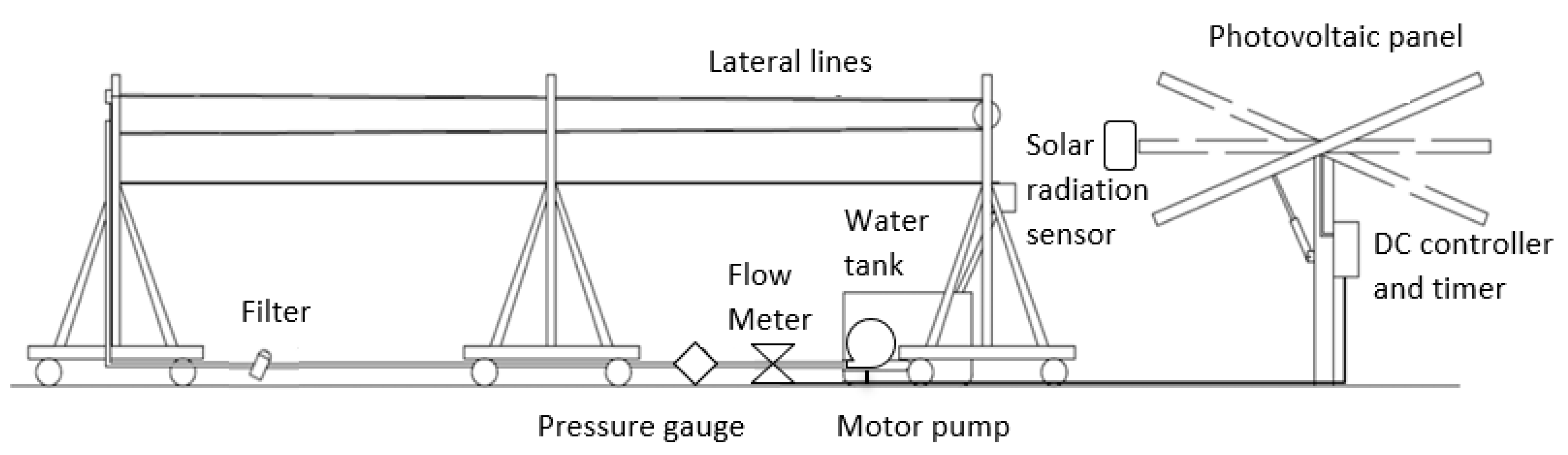
Figure 2.
- Electrical power supplied by pumping without a DC/DC converter, disconnected from irrigation.
Figure 2.
- Electrical power supplied by pumping without a DC/DC converter, disconnected from irrigation.
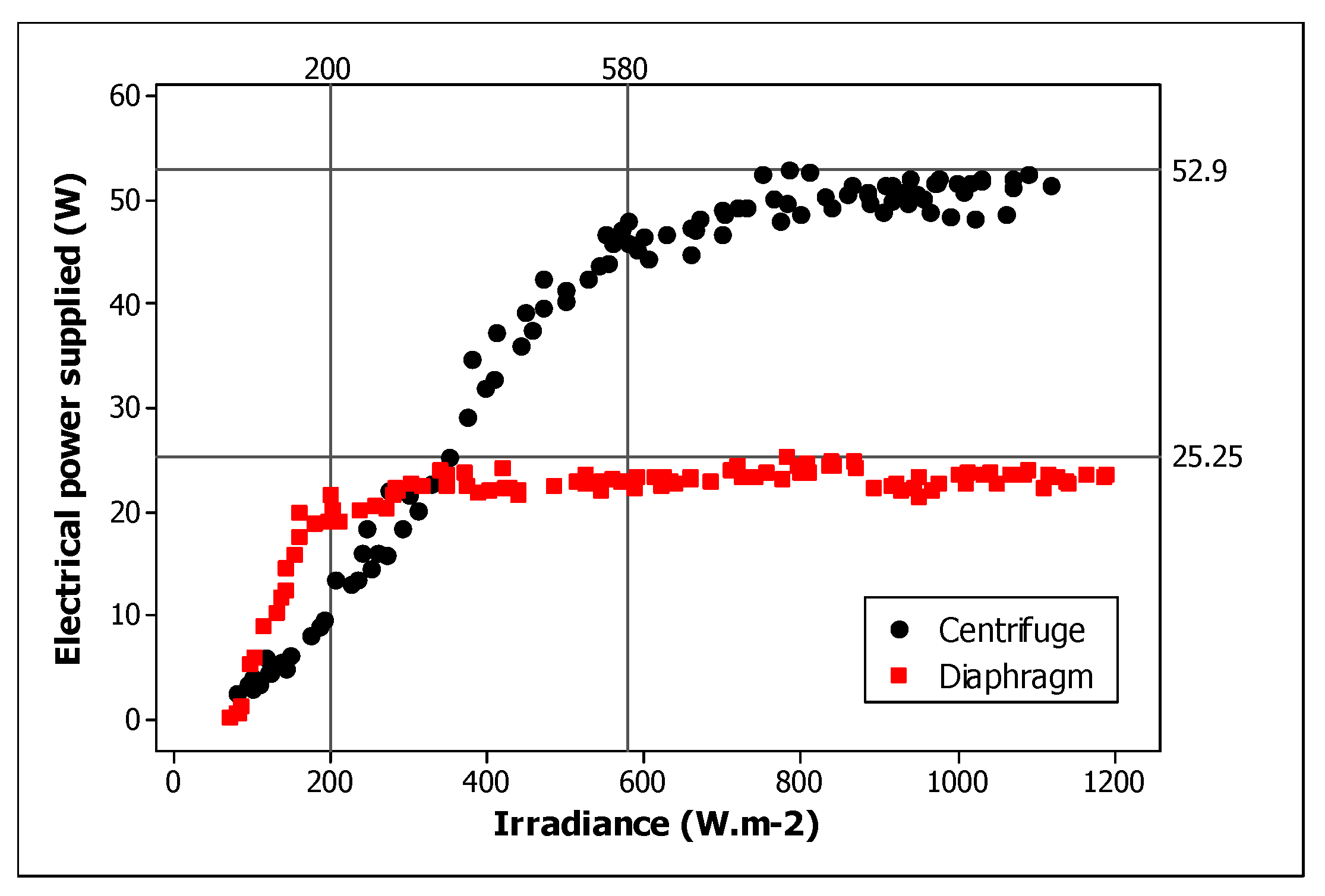
Figure 3.
– Maximum values of electrical power supplied .
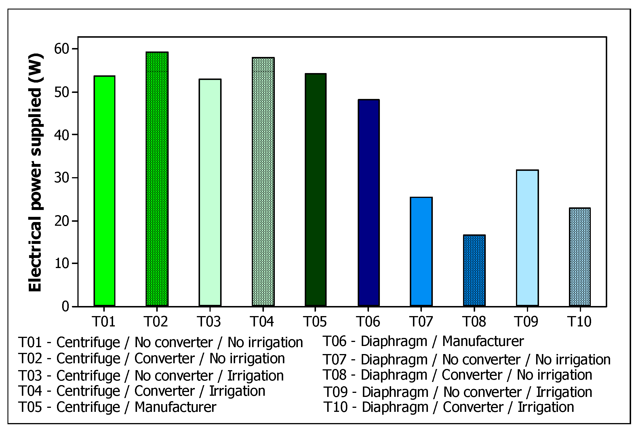
Figure 4.
Total head of the pumping system with a DC/DC converter (a) connected to irrigation and (b) disconnected from irrigation.
Figure 4.
Total head of the pumping system with a DC/DC converter (a) connected to irrigation and (b) disconnected from irrigation.
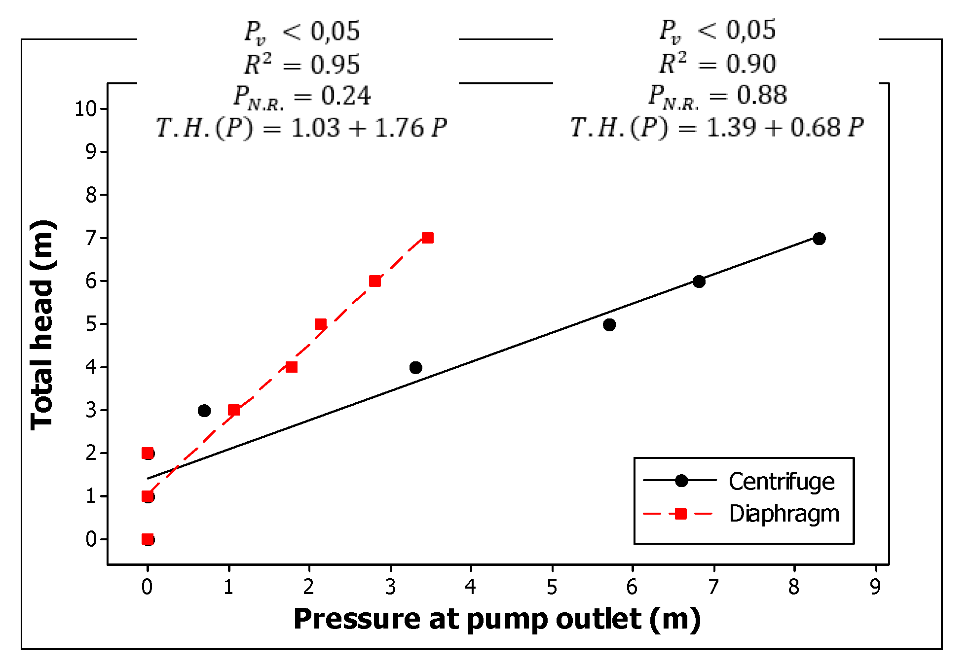
Figure 5.
Average total height.
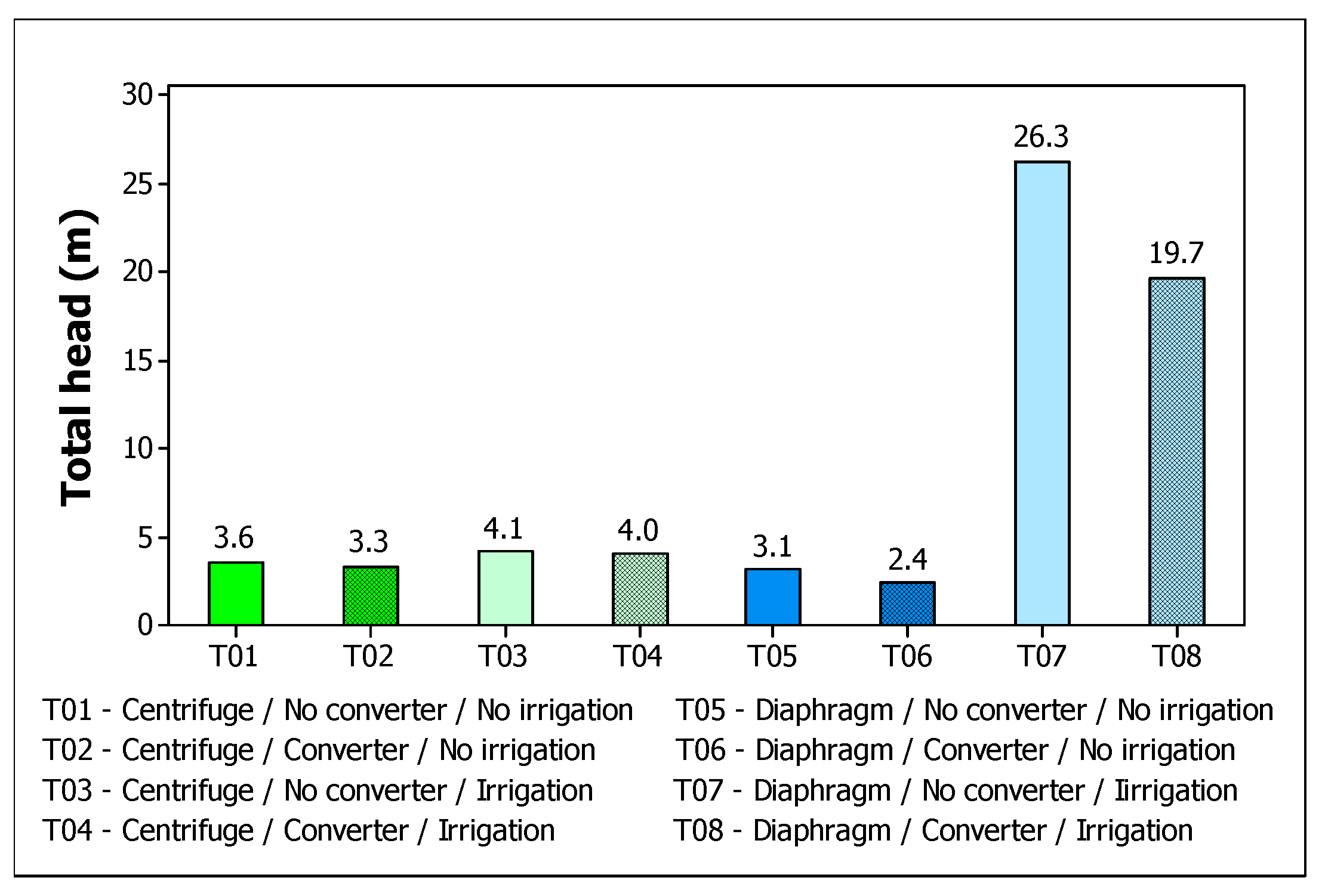
Figure 6.
Median total flows.
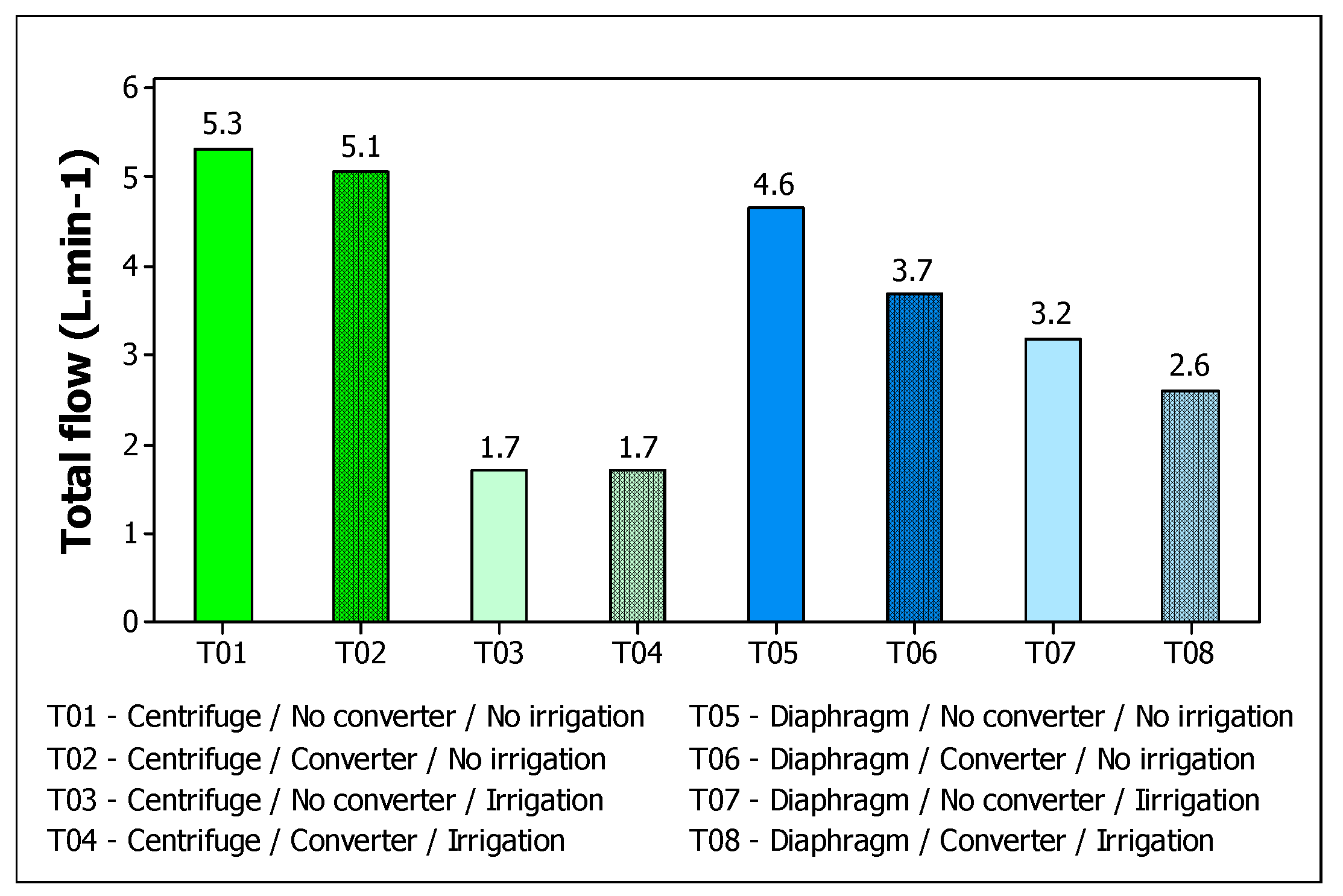
Figure 7.
Hydraulic power.
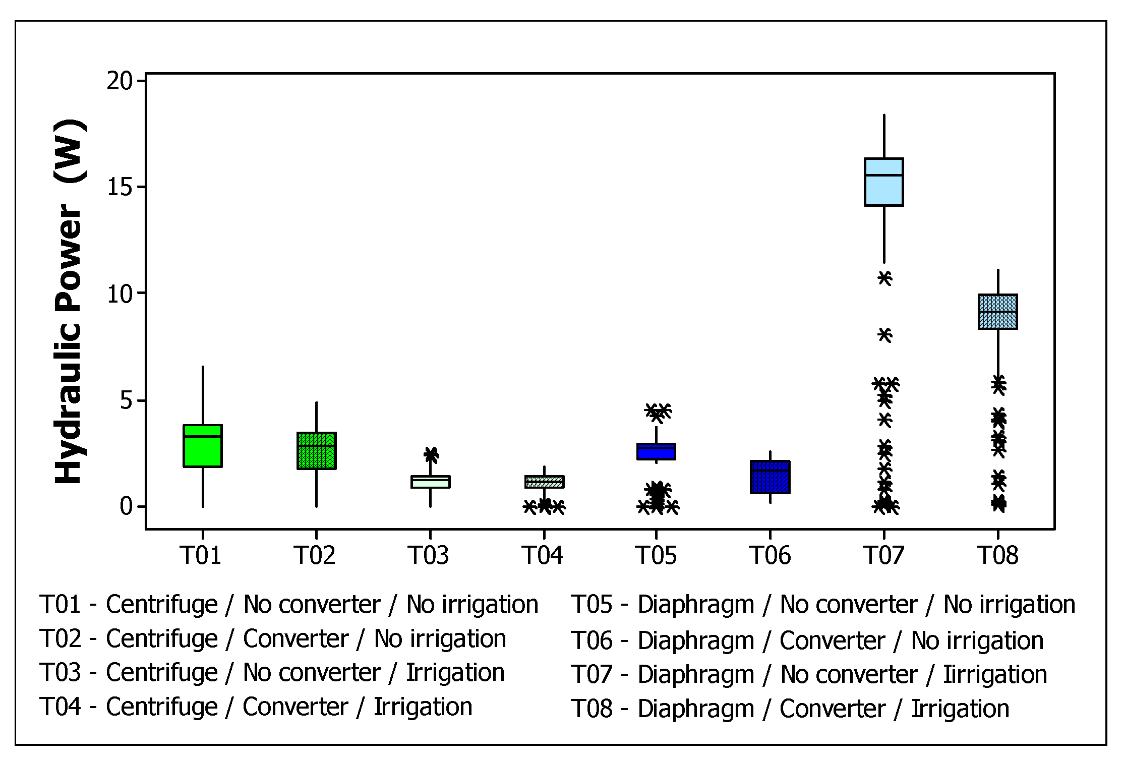
Figure 8.
Hydraulic power.
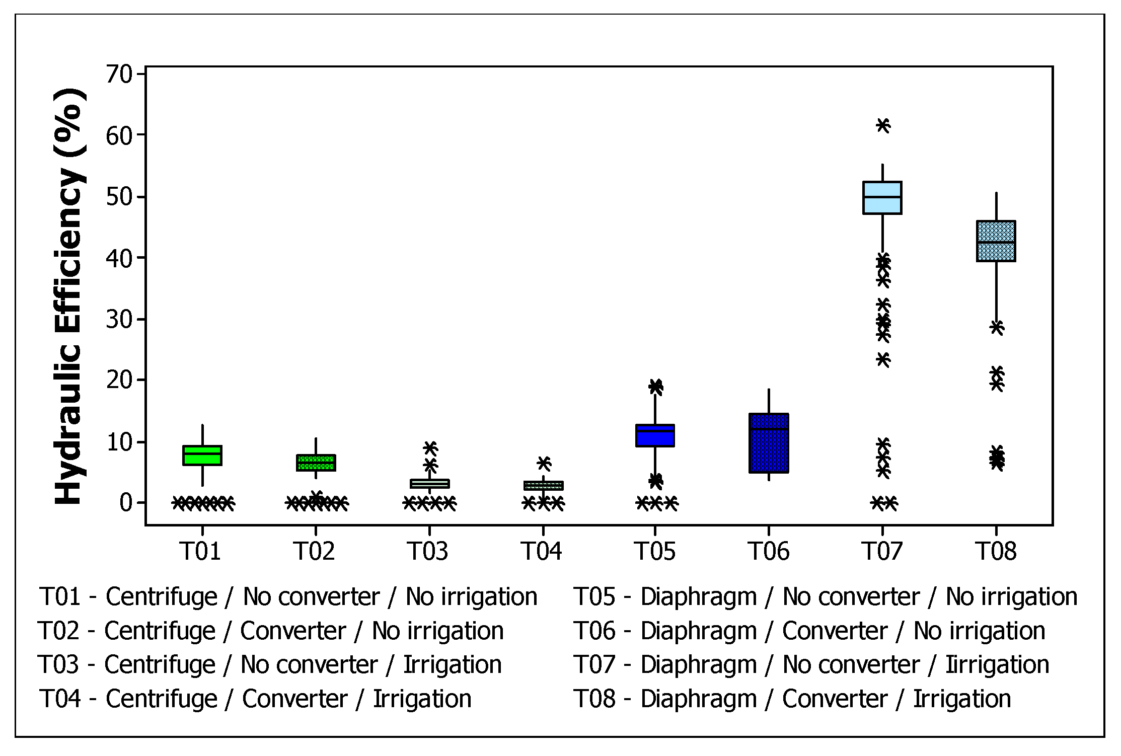
Figure 9.
Total efficiency.
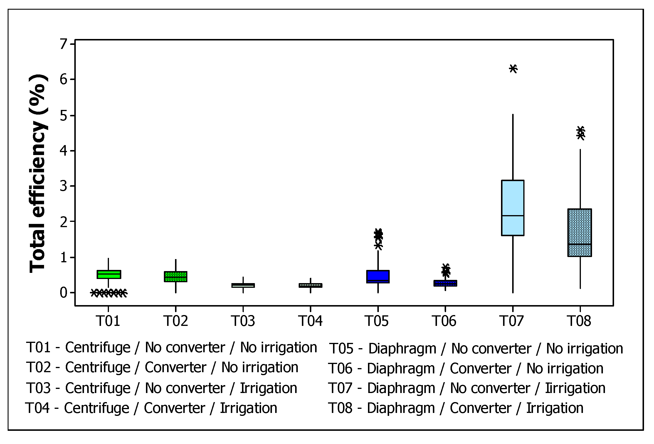
Figure 10.
- Voltage and current characteristics of the pump operating.
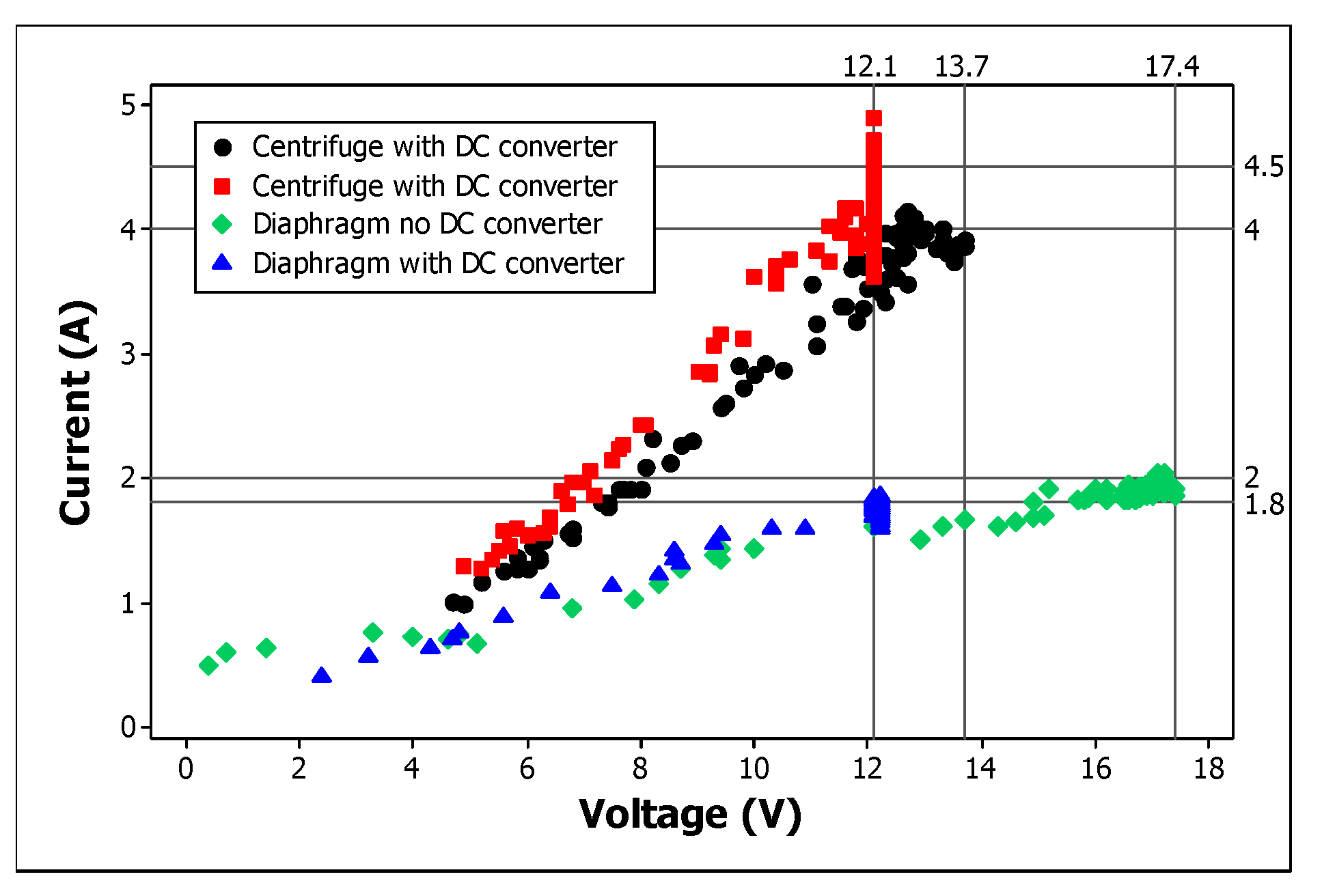
Figure 11.
- Superimposition of the current versus voltage curve for the pump with the curves for the photovoltaic panel.
Figure 11.
- Superimposition of the current versus voltage curve for the pump with the curves for the photovoltaic panel.
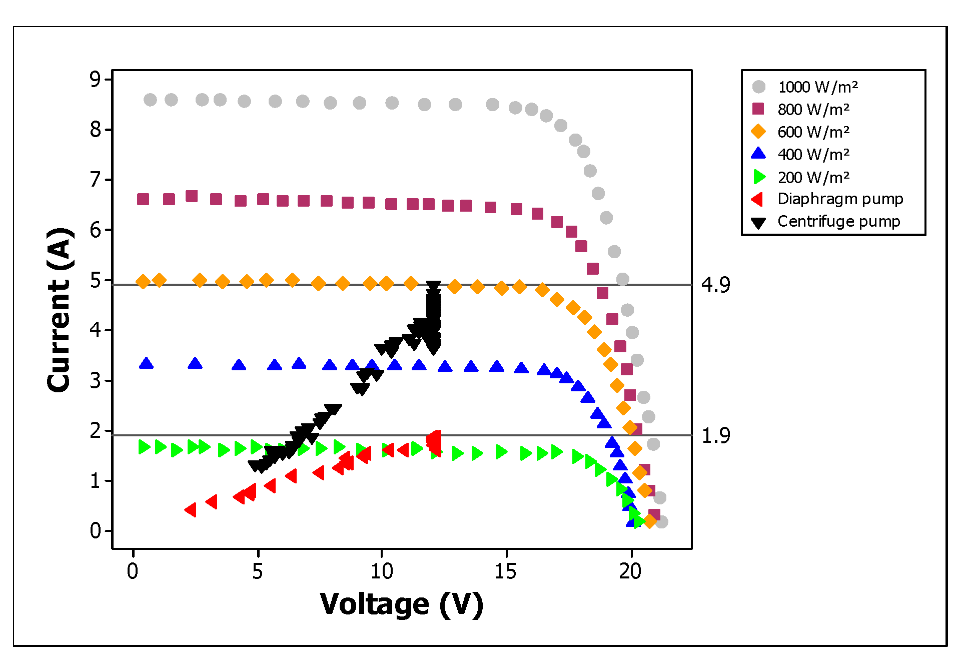
Figure 12.
- Hydraulic power vs. irradiance for the treatments connected to the lateral irrigation lines.
Figure 12.
- Hydraulic power vs. irradiance for the treatments connected to the lateral irrigation lines.
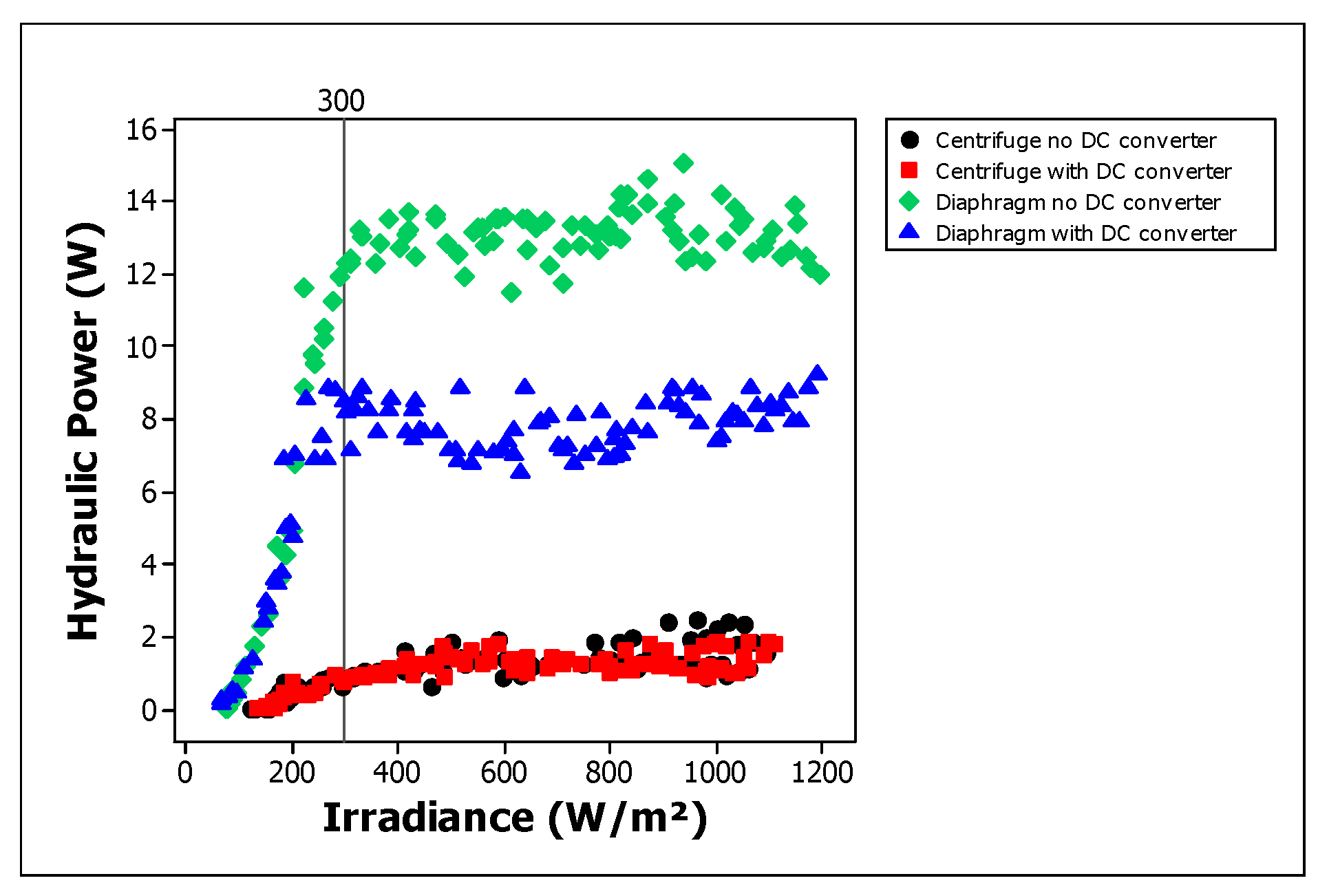
Figure 13.
- (a) Shewhart control chart and (b) exponential weighted moving average (EWMA) chart, of the DUC of irrigation with potable water and continuous application.
Figure 13.
- (a) Shewhart control chart and (b) exponential weighted moving average (EWMA) chart, of the DUC of irrigation with potable water and continuous application.
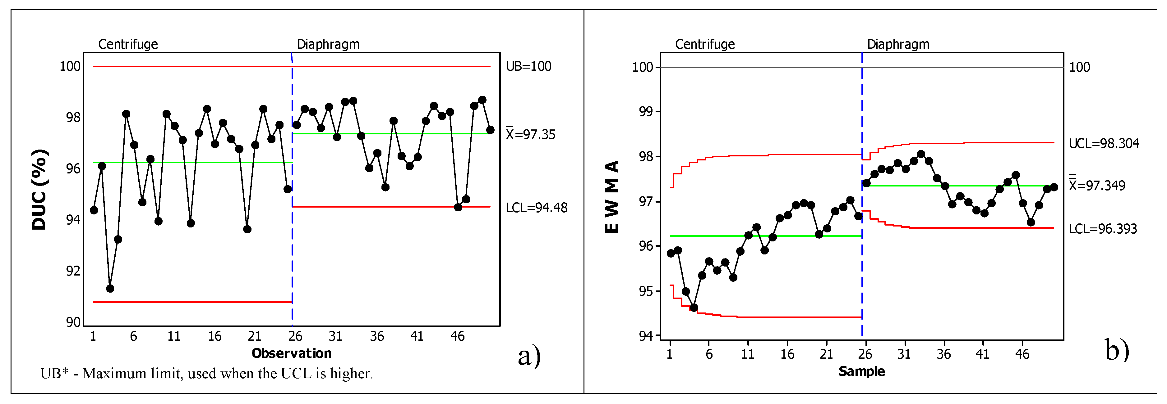
Figure 14.
– (a) Shewhart control chart and (b) exponential weighted moving average (EWMA) chart, of the DUC of irrigation with saline water and pulsed application.
Figure 14.
– (a) Shewhart control chart and (b) exponential weighted moving average (EWMA) chart, of the DUC of irrigation with saline water and pulsed application.
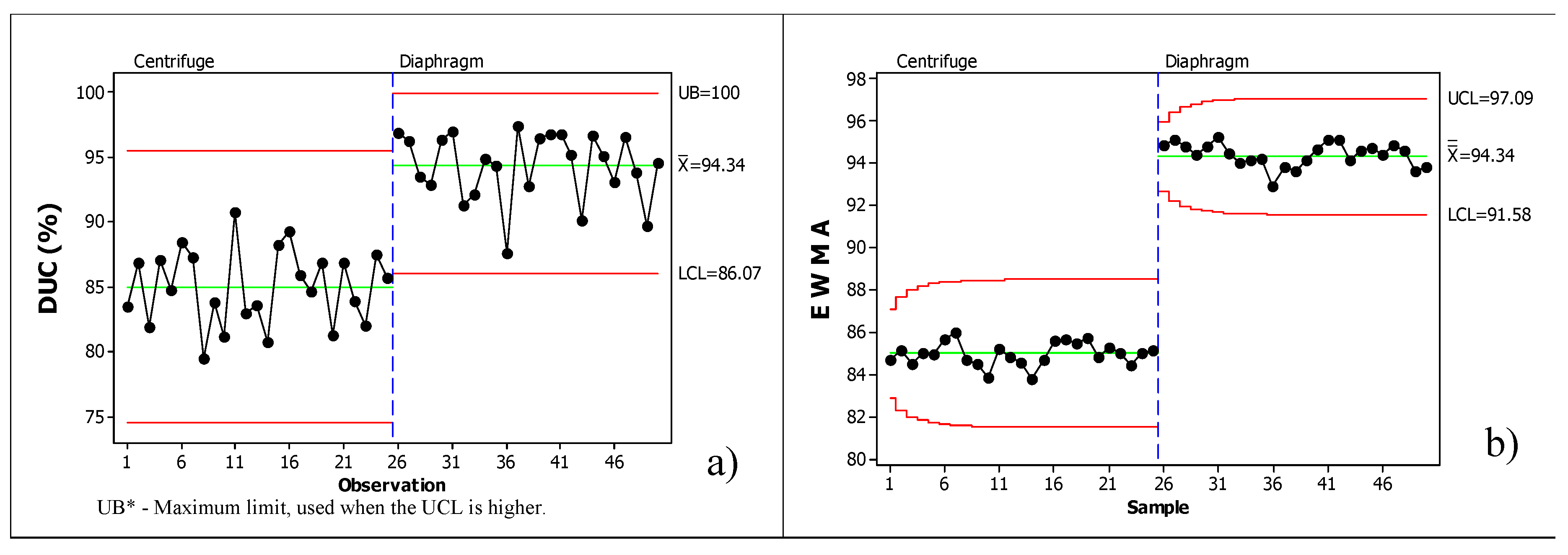
Figure 15.
– State of the filter and the last emitters of the lateral line after the end of the tests.
Figure 15.
– State of the filter and the last emitters of the lateral line after the end of the tests.
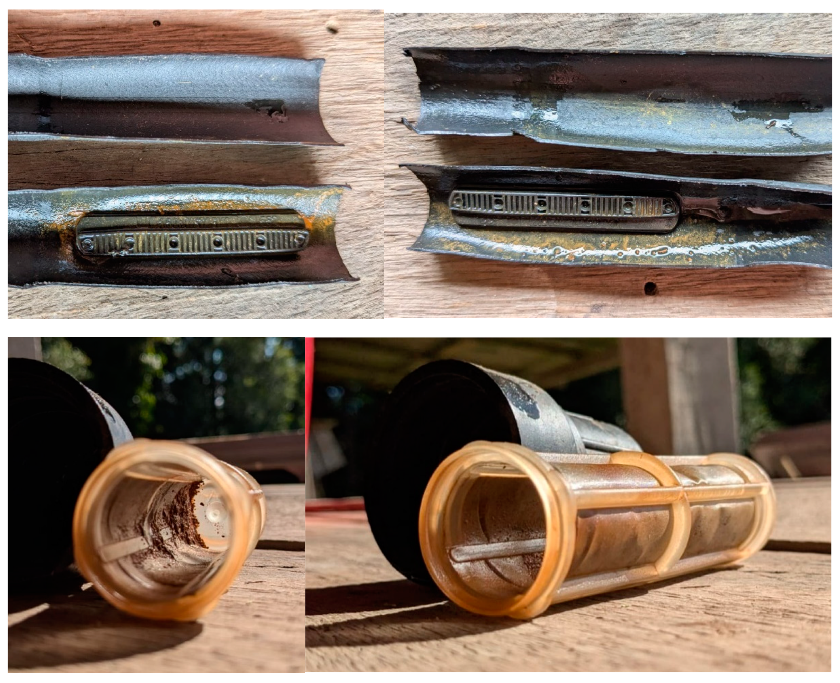

Table 1.
- Measuring instruments and their accuracy.
| Parameter | Instrument | Measuring range (accuracy) |
|---|---|---|
| Flow | RainPoint Smart HCS008FRF | 20 - 2400 L. (5%) |
| Pressure | DN63 REF 3822 - GENEBRE | 0 – 2.5 bar (2,5%) |
| Irradiance | SM206 | 1 – 3999 W. (5%) |
| Voltage | M430 DSN VC288 DC 0100 V 10A | 0-100 V (1%) |
| Current | M430 DSN VC288 DC 0100 V 10A | 0-10 A (1%) |
Table 2.
- Characteristics of the RS6E 150P photovoltaic module.
| Maximum power | 150 W |
| Open circuit voltage | 22.3 V |
| Short-circuit current | 8.82 A |
| Maximum power point voltage | 17.91 V |
| Maximum power point current | 8.38 A |
| Efficiency (module area) | 15.29% |
| Number of cells | 36 [4x9 (156x156 mm)] |
| Cell type | Polycrystalline, 4 or 5BB |
| Module dimensions | 1487 x 666 x 35 mm |
*All electrical characteristic parameters were tested under STC conditions: 1000 W/m², AM1.5, 25°C. Source: Resun Solar Energy 2024. Source: Gilbert e Ford (1986). Source: (Kolhe et al. 2004).
Table 3.
- Physico-chemical parameters of the saline water used in the pulsed drip experiment.
| Clogging factor | Severe Risk | Sample | Water quality | Severe use restriction | Sample |
|---|---|---|---|---|---|
| Suspended Solids | > 100 mg. | 112 mg. | Conductivity (EC) | > 3.0 dS. | 9.84 dS. |
| Dissolved Solids | > 2000 mg. | 5082 mg. | Nitrogen () | > 3 mg. | 1280.1 mg. |
| Total iron | > 1.5 mg. | 261.6 mg. | RAS | > 9 | 15,4 |
| Manganese | > 1 mg. | 366.8 mg. | Sodium | - | 231 mg. |
| ph | > 8.0 | 4.97 | Calcium | - | 264 mg. |
| Magnesium | - | 186.8 mg. |
Source: Gilbert e Ford (1986).
Table 4.
Performance factors, equations, and variables.
| Factors | Equation | Variables | N of equation |
|---|---|---|---|
| Solar power |
- Solar power (W) A - Area of the photovoltaic panel (m²) Irr - Irradiance (W. |
02 | |
| Electrical power |
- Electric power (W) I - electric current (A) U - voltage (V) |
03 | |
| Hydraulic power |
- Hydraulic power (W) ρ - Specific mass of water (kg) g - Gravitational strength (m. ) H - Height (m.c.a.) |
04 | |
| Motor pump efficiency |
- Motor pump efficiency (%) is the electrical power is the hydraulic power |
05 | |
| Total efficiency |
- Total efficiency (%) is the electrical power is the solar power |
06 |
Source: (Kolhe et al. 2004).
Table 5.
- Criteria for classifying DUC.
| Rating | DUC (%) |
| Excellent | > 90 |
| Good | 85 – 90 |
| Acceptable | 65 – 85 |
| Poor | < 65 |
Source: (Keller and Bliesner 1990).
Table 6.
- Performance characteristics of centrifuge and diaphragm pumps.
| Centrifuge | Diaphragm | |||||
| Height (M) | Manufacturer | Photovoltaic pumping | Manufacturer | Photovoltaic pumping | ||
| Flow (L.) | Flow (L.) | Pressure* (m) | Flow (L.) |
Flow (L.) | Pressure* (m) | |
| 0 | 31.0 | 15.5 | 0.0 | 4.1 | 4.9 | 0 |
| 1 | 25.1 | 14.0 | 0.0 | 3.9 | 4.8 | 0 |
| 2 | 23.9 | 12.1 | 0.0 | 3.75 | 4.7 | 0 |
| 3 | 20.0 | 9.9 | 0.7 | 3.63 | 4.7 | 1.07 |
| 4 | 16.0 | 8.0 | 3.3 | 3.51 | 4.6 | 1.78 |
| 5 | 10.6 | 7.0 | 5.7 | 3.42 | 4.5 | 2.14 |
| 6 | 2.0 | 2.8 | 6. | 3.35 | 4.5 | 2.80 |
| 7 | 0.0 | 0.7 | 8.3 | 3.3 | 4.4 | 3.46 |
*Pressure at the pump outlet. Source: (Seaflo 2024).
Disclaimer/Publisher’s Note: The statements, opinions and data contained in all publications are solely those of the individual author(s) and contributor(s) and not of MDPI and/or the editor(s). MDPI and/or the editor(s) disclaim responsibility for any injury to people or property resulting from any ideas, methods, instructions or products referred to in the content. |
© 2025 by the authors. Licensee MDPI, Basel, Switzerland. This article is an open access article distributed under the terms and conditions of the Creative Commons Attribution (CC BY) license (http://creativecommons.org/licenses/by/4.0/).
Copyright: This open access article is published under a Creative Commons CC BY 4.0 license, which permit the free download, distribution, and reuse, provided that the author and preprint are cited in any reuse.


