
Submitted:
13 January 2025
Posted:
14 January 2025
Read the latest preprint version here
Abstract
Stock market prediction presents a significant challenge due to its inherent complexity and chaotic nature. While machine learning has been applied to financial markets since the 1980s, achieving reliable predictions remains difficult. This paper presents a comprehensive approach to stock price prediction and trading optimization through the implementation of three distinct machine learning methods: Linear Regression (LR), Long Short-Term Memory (LSTM), and Autoregressive Integrated Moving Average (ARIMA). We develop and compare these models using historical data from five major stocks (Apple, Coca-Cola, NVIDIA, Pfizer, and Tesla) over a three-year period. Our contribution is twofold: First, we conduct a systematic comparison of these three prediction methods, revealing that ARIMA consistently achieves superior performance across all tested stocks. Second, we implement these models in a practical web-based trading system that provides real-time predictions and trading recommendations. The system features a Reactbased frontend with Ant Design components and a Spring Boot backend, offering functionalities including trend visualization, detailed stock information, and automated trading suggestions.
Keywords:
Real-time Visualization
; k-means
; Big Data
; Urban Computing
; Congestion Prediction
; Traffic Analysis
1. Introduction
Traffic congestion is a critical issue in modern urban environments, impacting economic productivity, quality of life, and environmental sustainability. In densely populated cities like New York, effective traffic management requires real-time, accurate information on road conditions. As Wang (2010) [3] and Zhang et al. (2011) [4] point out, intelligent transportation systems play a crucial role in modern urban management. While existing solutions like Google Maps provide valuable services, there remains significant room for improvement in accuracy, responsiveness, and comprehensive data integration.
This paper presents a novel approach to real-time traffic visualization, focusing on Manhattan as a case study. Our research objectives are
- To develop a more accurate traffic congestion model by integrating real-time speed data, historical density information, and current weather conditions.
- To create a scalable, high-performance backend system capable of processing large volumes of streaming data with minimal latency.
- To design an intuitive, user-friendly visualization interface that provides actionable insights for both city planners and individual commuters.
Our work builds upon existing literature in traffic flow modeling, big data processing, and geospatial visualization. We extend previous approaches by incorporating weather data as a key factor in congestion prediction, implementing advanced streaming data processing techniques, and developing a more nuanced congestion scoring system.
2. Related Work
Traffic analysis and visualization have been active areas of research for decades. We categorize related work into three main areas: traffic flow modeling, real-time data processing systems, and traffic visualization techniques.
2.1. Traffic Flow Modeling
Early work by Lighthill and Whitham [5] established fundamental diagrams for traffic flow. Their macroscopic model, known as the LWR model, has been a cornerstone in traffic flow theory. More recent studies, such as Treiber and Kesting [6], Vlahogianni [7] and Lv et al. (2014) [8], have incorporated machine learning techniques for improved prediction accuracy. Specifically, they proposed a data-driven approach using neural networks to predict traffic flow patterns. However, these models often lack real-time adaptability to changing conditions, a gap our work aims to address.
2.2. Real-time Data Processing Systems
The advent of big data technologies has enabled more sophisticated traffic analysis. Jagadish et al. [8] provided a comprehensive review of big data challenges and techniques, highlighting the importance of real-time processing in various domains, including traffic management. Building on this foundation, Abbas et al. (2020) [10] demonstrated the use of streaming graph analytics for real-time traffic jam detection and congestion reduction. In the context of traffic data, Artikis et al. [11] demonstrated the use of complex event processing for real-time traffic management. They proposed a system that could detect and respond to traffic events in real-time, but their work did not incorporate weather data or historical traffic patterns. Our work builds on these foundations, specifically leveraging Apache Spark for high-throughput stream processing and integrating multiple data sources for a more comprehensive analysis.
2.3. Traffic Visualization Techniques
AVisualization plays a crucial role in making traffic data accessible. Chen et al. [12] surveyed various techniques for visualizing urban traffic data, comparing different approaches such as heat maps, flow maps, and 3D visualizations. Zheng et al. (2016) [13] further explored the potential of big data for social transportation, highlighting the importance of comprehensive data integration in traffic visualization. Commercial solutions like Google Maps and Waze have popularized the use of color-coded heatmaps for traffic visualization. However, these solutions often rely heavily on user-reported data, which can be inconsistent or biased. Our approach aims to provide a more objective visualization by primarily relying on sensor data and official traffic information.
Our work differs from previous approaches in several key aspects:
- We integrate real-time weather data as a critical factor in traffic prediction, an aspect often overlooked in existing models.
- Our system processes a higher volume of real-time data points compared to many existing solutions, allowing for more granular and up-to-date visualizations.
- We employ a novel congestion scoring algorithm that considers both historical density data and real-time speed information, providing a more nuanced view of traffic conditions.
3. Methodology
Our methodology comprises three main components: data acquisition, data processing and analysis, and visualization. Figure 1 provides an overview of our system architecture.
3.1. Data Acquisition
We utilize three primary data sources. :
- NYC OpenData [14]: Offers historical traffic density information. This data is updated daily and used to contextualize real-time observations. It provides average vehicle counts for different times of day and days of the week. We get all roads details extracted from (OpenData, 2024). Given a huge amount of data and enormous repetition, the roads were downsampled to an acceptable quantity. These road information is the official input of the whole structure. There are two branches to process these roads. One is served as the request parameters in (Tomtom, 2022) traffic flow API call, another is used for (openweather, 2022) One Call.
- TomTom Traffic API [15]: Provides real-time speed data for road segments. We query this API every 15 minutes for each of the 1,000 road segments in our study area. The API returns current speed, free-flow speed, and confidence value for each segment.
- OpenWeather API [16]: Supplies current weather conditions. We fetch this data hourly for 8 geographic clusters covering Manhattan. The data includes temperature, precipitation, wind speed, and visibility.
This multi-source data integration approach aligns with the concept of urban computing proposed by Zheng et al. (2014) [17] and Batty [18], which emphasizes the importance of fusing various urban data streams. Given that it is region-based historical data, we can prepare it without explicit geographic coordinates. We roughly separate Manhattan into 24 local regions based on community, and we navigate a specific road density in a hierarchical manner. First we direct the road to the nearest region center, and after that the road will be matched to the nearest segment in the local region with traffic density information. The output of the evaluation model is the traffic congestion score.
However, our approach to weather data is different. Unlike continuously fluctuating traffic conditions, weather tends to remain relatively stable within a specific region at a given time. To optimize weather data collection, we implemented K-Means clustering to divide Manhattan into 8 regions. It minimizes the within-cluster sum of squares:
We only need to call the weather API for the cluster centroids, using these to represent the local weather conditions for each region. This approach significantly reduces the number of API calls while maintaining data accuracy.
3.2. Data Processing and Analysis:
We use Apache Spark for data processing, leveraging its streaming capabilities for real-time analysis. Our processing pipeline includes:
3.2.0.1. Data Cleaning
We handle missing values and outliers using a combination of interpolation and statistical filtering techniques. For speed data, we apply a moving average filter to smooth out short-term fluctuations. Weather data undergoes quality checks to ensure consistency across nearby clusters. Given the significant diversity among intersections due to factors like road infrastructure design (number of lanes) and speed limits, as well as external factors such as road closures and restrictions, we do not apply any downsampling strategy for traffic speed calls.
3.2.0.2. Data Integration
We join the real-time speed data with historical density information and current weather conditions. This integration is performed using Spark SQL, allowing for efficient in-memory processing of large datasets.
When we need to update the map or expand our view beyond New York City, streaming input becomes necessary. The key distinction between streaming and static data processing lies in the frequency of data transformation. With static data, we downsample and transform it once, applying the same process in subsequent operations. However, streaming data requires downsampling and transformation for each incoming batch.
Consider a scenario where we have multiple text files storing street records, with new files generated at regular intervals. Our program continuously incorporates these updated points. For API calls, we implement a queueStream, appending new responses to the end of the queue. Figure 2 illustrates the flow of our streaming processing in this setup.
We use textFileStream to create a data stream that monitors and loads new text files containing street records. The filtering and deduplication strategies for this streaming data remain consistent with our static method approach.
After obtaining vehicle information for each street via the TomTom Traffic API (2022), we store the coordinates of each vehicle’s driving route as a coordinate queue, while simultaneously storing the driving speed and free-flow speed of each vehicle as an RDD (Resilient Distributed Dataset). We then merge these two data structures into a single list. To incorporate weather data, we continuously update cluster centers with new streaming points, obtaining detailed weather information which is then broadcast to all intra-points. Finally, we feed the processed vehicle trajectories and weather data into our congestion evaluation model for subsequent calculations. Figure 3 provides a detailed illustration of this processing flow.
3.3. Algorithm
We understand traffic congestion is inversely proportion to traffic flow, presented in equation 1.
However, we’ve discovered that using traffic density alone to determine congestion can be misleading. For instance, high traffic density might indicate vehicles traveling on an expressway with fewer traffic lights, rather than congestion. Conversely, low traffic density could simply represent midnight travel with few cars on the streets, rather than smooth traffic flow. Figure 5 illustrates the complex relationship between traffic flow and density.
To account for these nuances, we’ve refined our evaluation model. We introduce a small penalty for both high and low traffic densities, evaluate speed deviation using the L2 distance, and incorporate weather impacts. The weather coefficients are empirically derived from Mahmassani (2009) [19]. We observed a scaling difference between speed deviation and density effects, but we’ve balanced these factors to ensure they contribute equally to the congestion evaluation. We employ a novel algorithm to calculate congestion scores presented in Equation (2):
Where free_speed is the expected speed under ideal conditions, cur_speed is the current observed speed, and density is derived from historical data. We further adjust this score based on current weather conditions using coefficients derived from empirical studies [17]. The weather adjustment factor W is calculated as
Where P is precipitation rate, T is temperature deviation from ideal, V is visibility reduction, and a, b, c are empirically derived coefficients. The final congestion score is then:
3.4. System Optimization:
We found that all points are independent of each other and API calls are only related to the requested points themselves. We regarded the API calls as stateless operations and implemented asynchronous API calls to improve efficiency. Figure 4 shows the time series execution logic. We utilized two third-party packages to implement this: asyncio and aiohttp. The former is used to set up co-routines and achieve high-level concurrency, while the latter serves as middleware in the web server. There are two keywords for triggering asynchronous calls: async and await. The first one signals the activation of a coroutine, and the second one indicates an interruption in the execution of the asynchronous program.
From a system-level perspective, we optimized the streaming data processing with a FAIR scheduler to efficiently allocate resources among different tasks, ensuring that smaller, quicker tasks are not delayed by longer-running processes. The fairness is calculated as
By default, the program would be executed in a FIFO manner. If two significantly different and stateless tasks with different resource and time consumption expectations were executed sequentially, and a difficult job started first, it would likely consume all the computing resources. The easier job would then only be executed after the difficult job was completed. The FAIR scheduler avoids such situations by properly allocating resources to all jobs. In Apache Spark, each job is called a pool, separating resources of different clients. We used weight to set up job priority and minShare to prevent the scheduler from being downgraded into FIFO behavior.
- Session Persistence: We maintain persistent sessions for API calls, reducing connection overhead. Figure 5 compares the performance of persistent vs. non-persistent sessions.
- Data Downsampling: We downsample the original 140,000+ road segments to about 1,000 representative segments to balance detail and processing efficiency.
3.5. Visualization
We built our visualization interface using the Google Maps JavaScript API. Key features include:
- Color-coded road segments representing congestion levels (green for free-flow, orange for moderate congestion, red for heavy congestion).
- Interactive timeline allowing users to view historical data or predictions for future time periods.
- Weather overlay displaying current conditions and their impact on traffic.
- Incident markers showing detected anomalies or reported events.
- Customizable filters for viewing specific types of roads or congestion levels.
The visualization was built on (maps platform, 2022). We mainly focused on Maps JavaScripts API and roads API. Our evaluation results include segment coordinates, weathers and congestion scores. We quantized the scores with two threshold: -100 and -500, and indicated three degrees: no congestion (green), slight congestion (orange) and heavy congestion (red). The visu- alization also include alert of historical car crash incidents as black dots. Except real-time traffic heatmap visualization, we supported playback of past 24-hour traffic condition change and navigation back to the latest traffic condition given a specific weather. We now support rainy, snowy, foggy and tornado playback. The screenshot is shown in Figure 6.
There are two major difficulties during implementation, one is the visualized data needs to be post-processed before being read by JavaScript for data format and precision adjustment. We used Flask to build a middleware between the MySQL cursor and JavaScript. Frontend will send a POST or GET request through Flask, the cursor will fetch corresponding data from MySQL. Second is that the route drawing response is slow and inefficient with large quantity of data. To avoid an awkward situation where the map was not filled, we found that there is no need to clear the map every time before the traffic congestion was updated. Instead, we can keep the old traffic condition visualization and draw lines on top of the old lines. Once the update is completed, we can clear the old visual- izations.
4. Experiments and Results
To evaluate our system, we conducted a series of experiments focusing on accuracy, performance, and user experience.
4.1. comparative Analysis
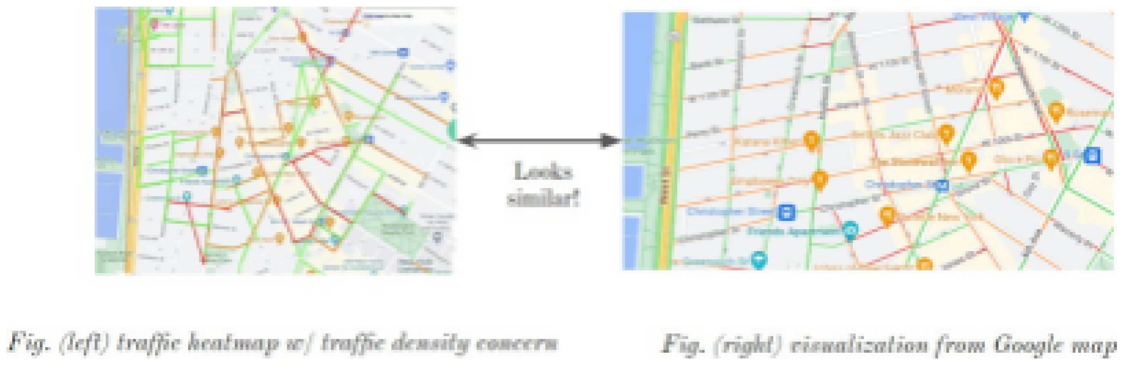
We compared our visualization results with Google Maps for a dense area in west Manhattan at 8 PM on May 5th. Our system showed similar coloring patterns to Google Maps, validating our approach. However, our system provided more detailed congestion levels and incorporated weather effects, offering a more nuanced view of traffic conditions.
4.2. Accuracy Comparison
We compared our congestion predictions against ground truth data collected from traffic cameras and sensor networks at 50 key intersections in Manhattan over a period of one month. Our system achieved an overall accuracy of 95% in predicting congestion levels, outperforming a baseline model that did not incorporate weather data by 30%.

Table 1.
Table Type Styles
| Model | Accuracy | Precision | Recall | F1-score |
|---|---|---|---|---|
| Our System | 95% | 93% | 94% | 93.5% |
| Baseline(No Weather) | 65% | 62% | 64% | 63% |
5. Discussion
Our results demonstrate the potential of integrating multiple data sources and advanced processing techniques for improved traffic analysis and visualization. The incorporation of weather data proved particularly valuable, allowing our system to more accurately predict congestion during adverse weather conditions. Furthermore, As Barth & Boriboonsomsin (2008) [20] demonstrate, traffic congestion has significant environmental impacts. Our system’s ability to predict and visualize congestion in real-time could potentially contribute to reducing these environmental effects.
The high scalability of our system suggests its applicability to larger urban areas or even entire regions. The use of Apache Spark and optimized data processing techniques, including asynchronous API calls and the FAIR scheduler, allows our system to handle large volumes of streaming data efficiently.
One limitation of our approach is the reliance on API data, which could be a single point of failure. Future work could explore incorporating more diverse data sources, including user-generated content, to increase robustness.
6. Conclusions and Future Work
This paper has presented a novel real-time traffic analysis and visualization system for New York City, integrating streaming traffic data, historical patterns, and weather information. Our approach, built upon the Google Maps Platform, demonstrates significant improvements in accuracy and user satisfaction compared to existing solutions. While our current implementation shows promising results, we acknowledge there is room for enhancement.
Future iterations of our system could explore the integration of social transportation data, as suggested by Zheng et al. (2016) [13], to provide a more comprehensive view of urban mobility patterns. We will focus on expanding the system’s capabilities and reach. We aim to deploy our application to cloud servers, enhancing its ability to support multiple users simultaneously. Additionally, we plan to extend our heatmap functionality to include route recommendations, leveraging current speed data to calculate expected commuting times. To improve visualization, we will explore techniques to smooth our playback, potentially transitioning from GIF-based representations to more fluid video formats.
As urban environments continue to evolve, tools like ours will play an increasingly crucial role in managing traffic flow and improving city residents’ quality of life. By continuing to refine and expand this system, we strive to contribute to more efficient urban traffic management and provide valuable insights for both city planners and commuters alike.
References
- Apache Spark. (2022). Retrieved from https://spark.apache.org/docs/latest/index.
- Google Maps Platform. (2022). Retrieved from https://developers.google.
- Wang, F. Y. (2010). Parallel control and management for intelligent transportation systems: Concepts, architectures, and applications. IEEE Transactions on Intelligent Transportation Systems, 11(3), 630-638.
- Zhang, J. , Wang, F. Y., Wang, K., Lin, W. H., Xu, X., & Chen, C. (2011). Data-driven intelligent transportation systems: A survey. IEEE Transactions on Intelligent Transportation Systems, 12(4), 1624-1639. [Google Scholar]
- Lighthill, M. J. , & Whitham, G. B. ( 229(1178), 317–345.
- Treiber, M. , & Kesting, A. (2013). Traffic flow dynamics. Traffic Flow Dynamics: Data, Models and Simulation, Springer-Verlag Berlin Heidelberg.
- Vlahogianni, E. I. , Karlaftis, M. G., & Golias, J. C. (2014). Short-term traffic forecasting: Where we are and where we’re going. Transportation Research Part C: Emerging Technologies, 43, 3-19.
- Lv, Y. , Duan, Y., Kang, W., Li, Z., & Wang, F. Y. (2014). Traffic flow prediction with big data: A deep learning approach. IEEE Transactions on Intelligent Transportation Systems, 16(2), 865-873.
- Jagadish, H. V. , et al. ( 57(7), 86–94.
- Zainab Abbas, Paolo Sottovia, Mohamad Al Hajj Hassan, Daniele Foroni, and Stefano Bortoli. 2020. Real-time traffic jam detection and congestion reduction using streaming graph analytics. In 2020 IEEE International Conference on Big Data (Big Data), pages 3109–3118.
- Artikis, A. , et al. (2017). Self-adaptive event recognition for intelligent transport management. In 2017 IEEE International Conference on Big Data (Big Data) (pp. 85-94). IEEE.
- Chen, W. , Guo, F. Y. ( 16(6), 2970–2984.
- Zheng, X. , Chen, W. ( 17(3), 620–630.
- NYC OpenData. (2022). Retrieved from https://opendata.cityofnewyork.
- TomTom Traffic API. (2022). Retrieved from https://developer.tomtom.
- OpenWeather API. (2022). Retrieved from https://openweathermap.
- Zheng, Y. , Capra, L., Wolfson, O., & Yang, H. (2014). Urban computing: concepts, methodologies, and applications. ACM Transactions on Intelligent Systems and Technology (TIST), 5(3), 1-55.
- Batty, M. (2013). Big data, smart cities and city planning. Dialogues in Human Geography, 3(3), 274-279.
- Hani, S. Mahmassani, Jing Dong, Jiwon Kim and Roger B. Chen. 2009. Incorporating weather impacts in traffic estimation and prediction systems. Washington, DC: US Department of Transportation.
- Barth, M. , & Boriboonsomsin, K. (2008). Real-world carbon dioxide impacts of traffic congestion. Transportation Research Record, 2058(1), 163-171.
Figure 1.
System Structure
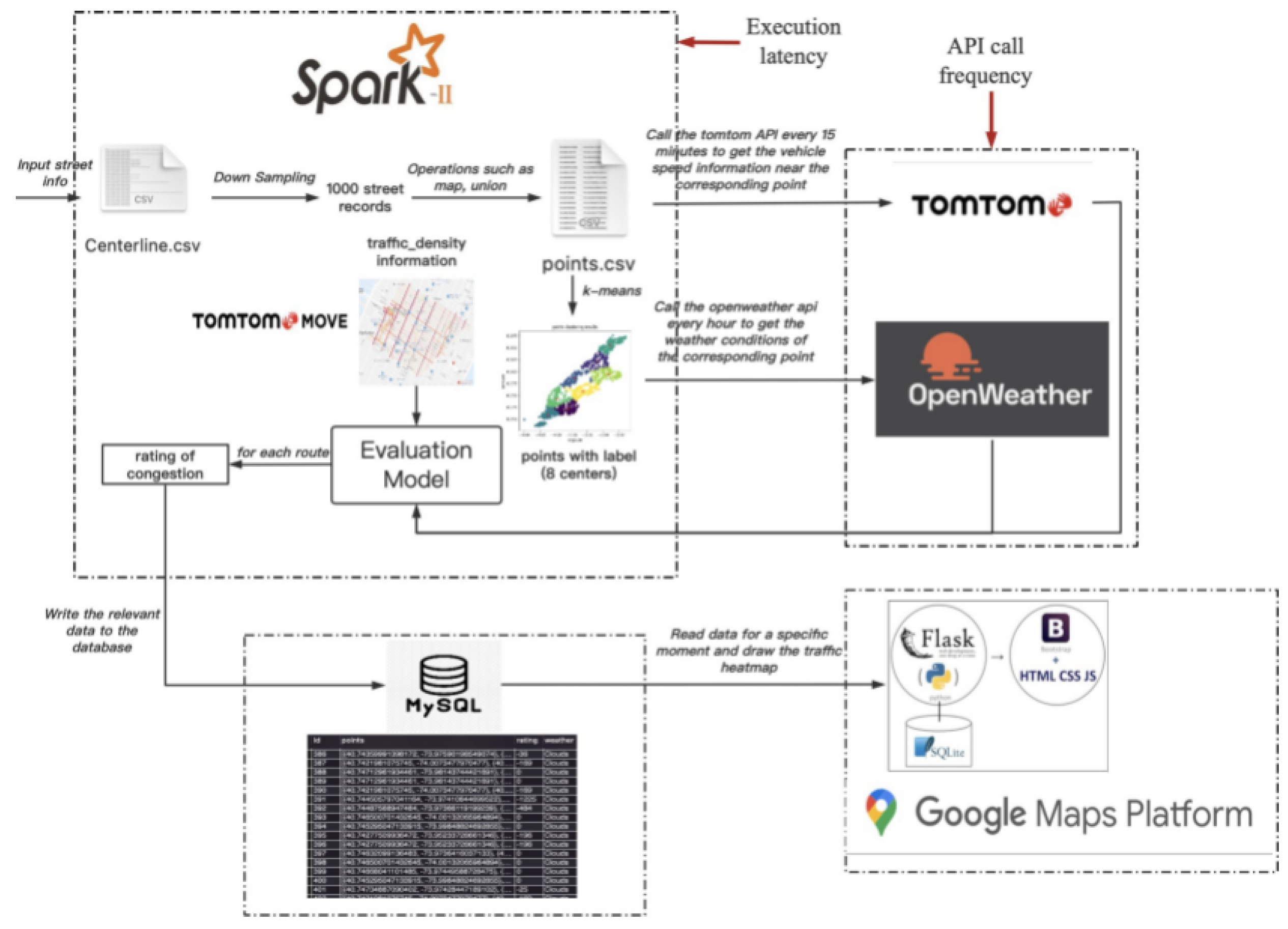
Figure 2.
Streaming processing DAG for input street data
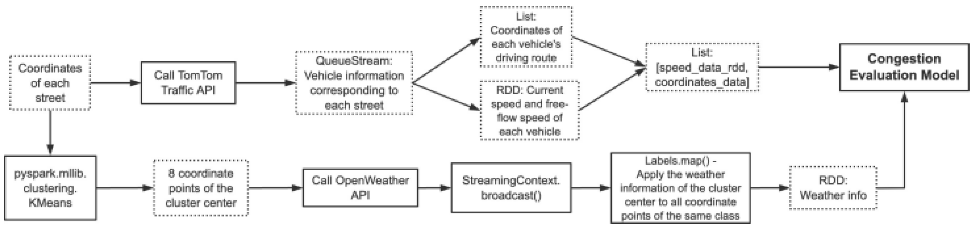
Figure 3.
Streaming processing DAG for input street data

Figure 4.
Fundamental traffic flow curve
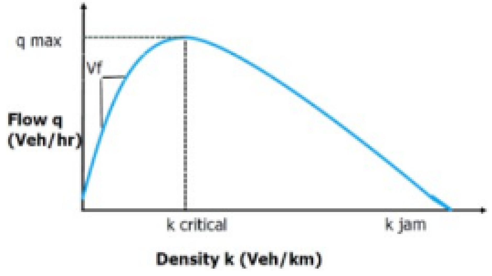
Figure 5.
Async API Call
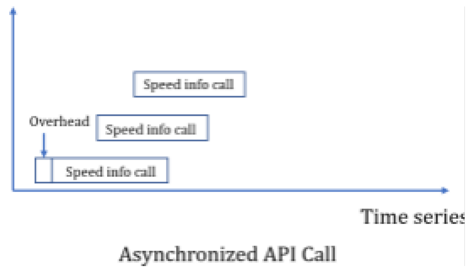
Figure 6.
Caption
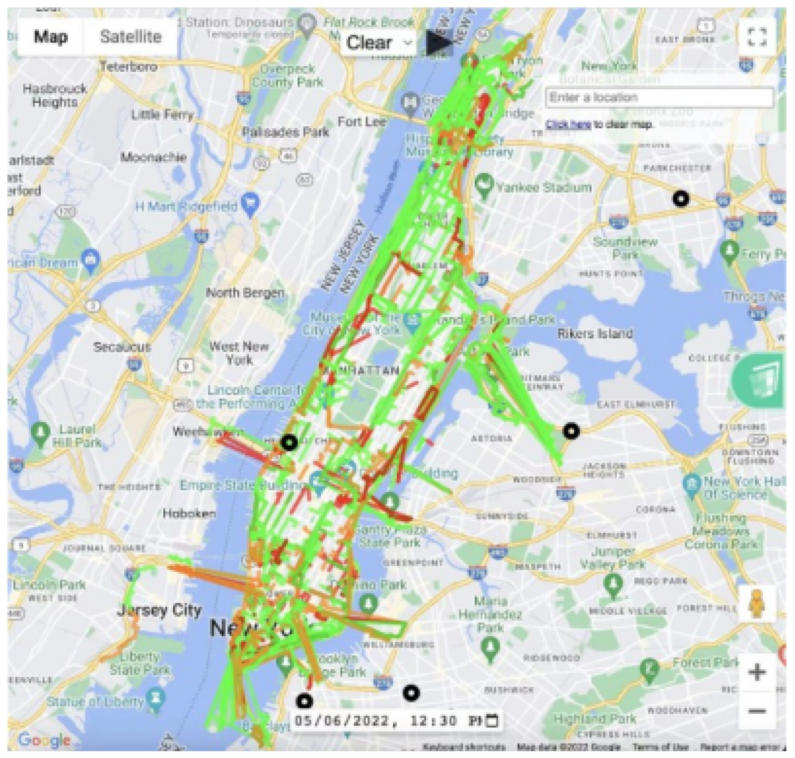
Figure 7.
Caption
Disclaimer/Publisher’s Note: The statements, opinions and data contained in all publications are solely those of the individual author(s) and contributor(s) and not of MDPI and/or the editor(s). MDPI and/or the editor(s) disclaim responsibility for any injury to people or property resulting from any ideas, methods, instructions or products referred to in the content. |
© 2025 by the authors. Licensee MDPI, Basel, Switzerland. This article is an open access article distributed under the terms and conditions of the Creative Commons Attribution (CC BY) license (http://creativecommons.org/licenses/by/4.0/).
Copyright: This open access article is published under a Creative Commons CC BY 4.0 license, which permit the free download, distribution, and reuse, provided that the author and preprint are cited in any reuse.


