
Submitted:
11 January 2025
Posted:
15 January 2025
You are already at the latest version
Abstract
Accurate forecasting of exchange rates plays a huge role in the lives of the vast majority of the population. The work of various businesses, policymakers and economists is extremely dependent on the right tools for forecasting exchange rates, due to their significant implications for domestic and foreign trade, investment strategies, and economic planning. This paper focuses on modelling daily exchange rates between Kyrgyz som (KG som) and US dollar, and compares the actual data with developed forecasts using time series analysis over the period from 2010 to 2023. The official daily currency exchange data of National Bank of the Kyrgyz Republic is processed in the study. Three ML algorithms, Random Forest regressor, CatBoost regressor and multiple linear regression (MLR), are compared with triple exponential smoothing (Holt-Winters) and Prophet models. The goal of the study is to define how effectively the above methods predict changes in the exchange rate of the KG som to the US dollar. The accuracy of the forecasts is evaluated by Mean Absolute Error (MAE), and Mean Absolute Percentage Error (MAPE). This study can be considered as the first academic study on time series forecasting of the national currency of Kyrgyzstan. The implicit idea of the work is to open up this area to researchers. Therefore, the study can be extended in the future by adding other methods and models.
Keywords:
Time series
; forecasting
; exchange rate
; Kyrgyz som
; machine learning
1. Introduction
Today in the global economy, the research in the field of currency exchange rate (CER) forecasting plays a key role due to its significance in managerial and financial decision making. Accuracy in forecasting currency exchange rates is important in many fields: international trade, investments, policy making, transnational businesses and global markets. Currency Exchange provides a rate of currencies in pair of currency of two countries e.g. USD to KGS for U.S. Dollar and Kyrgyz som. According to this rate, all stakeholders and agents buy or sell on the foreign exchange.
The Kyrgyz Republic, a mountainous country in Central Asia, has undergone significant economic transformation since receiving independence from the Soviet Union in 1991. The main sectors of the economy of Kyrgyzstan are: agriculture, mining, garment industry, and services [1] [pp 43-50]. Other sources of income include migrant remittances and foreign aid [2] [pp 2-24]. The Kyrgyz som (KGS), introduced in 1993, has experienced various degrees of volatility due to internal economic policies, external economic shocks, and regional geopolitical dynamics.
This Thesis utilizes a range of time series forecasting methods, including traditional approaches such as exponential smoothing and Prophet, as well as advanced machine learning-based techniques, decision tree ensembles, and linear regression. These models are trained on historical exchange rate data over the period of 14 years (2010–2023).
The main goal of this study is to compare the effectiveness of several models in predicting the KGS exchange rate volatility against the US dollar. By evaluating the performance of different forecasting methods, the study helps identify a leading model. This research can be considered as the first academic work on KGS time series analysis and forecasting.
The thesis has the following structure:
- Chapter 1 is an introductory part to the topic. It provides some economic context of Kyrgyzstan and defines the main objective of the study.
- Chapter 2 reviews the existing literature on time series analysis and forecasting.
- Chapter 3 is devoted to methodology—the practical implementation of various models based on the currency data.
- Chapter 4 is a combination chapter of presenting the results and their interpretation, discussion and conclusions.
2. Background
2.1. Time Series Forecasting
Historically, time series (e.g. CER) forecasting has been approached by various disciplines, including economics, statistics, and mathematics. In the past, traditional econometric models, such as ARIMA (autoregressive integrated moving average and its types) and VAR (vector autoregression), have been widely used for time series prediction. Besides, such models provided relatively accurate results with respect to exogenous factors, e.g. interest rates, inflation, or GDP level [1]. However, the volatility and complexity of CER fluctuations require new solutions. Rapidly developing machine learning (ML) and deep learning (DL) techniques are providing a new approach to time series forecasting problems.
2.2. ARIMA
ARIMA is a family of time series forecasting methods that includes not only ARIMA itself, but also methods such as SARIMA and SARIMAX. ARIMA (autoregressive integrated moving average) contains of three major components: AR–the number of past values as lags, I–means that data is stationary, and MA–the calculation of past forecasting errors [3] [p. 525]. Other forms and extensions of ARIMA methods can take into account such variables as seasonality, trend, and exogenous factors.
The main disadvantage of ARIMA models is the complexity of their application. The entire implementation process includes such steps, as checking the time series data for stationarity using Augmented Dickey Fuller (ADF), KPSS, or other statistical tests; in case of non-stationary - complex transformation of data into stationary; utilizing ACF (autocorrelation function) and PACF (partial autocorrelation function) to find right parameters for non-seasonal and seasonal order [3] [p. 529]. Whereas ARIMA methods have a strong statistical background, can capture various types of time series’ patterns and behaviors, they’re still weak to handle non-linear data with complex relationships. Additionally, these methods are time-consuming and require specific knowledge of statistics [4] [p. 1395].
2.3. Exponential Smoothing
Exponential smoothing methods are widely used in time series forecasting due to their effectiveness in short-period forecasting. These models are relatively simple. Their components and parameters are intuitively understandable. Another advantage is that exponential smoothing requires only limited data storage and computational effort.
Compared to classic ARIMA, exponential smoothing shows relatively good accuracy [5] [p. 3]. Methods such as triple exponential smoothing are available to work with limited historical data, and show relatively high effectiveness in predicting time series with relatively large noise in data. Additionally, unlike linear regression-based models (such as ARIMA), exponential smoothing methods can be adjusted to account for effects such as trend line decay over time (damped trend).
2.4. Machine Learning
According to Masini et al., machine learning (ML) methods are “the combination of automated computer algorithms with powerful statistical methods to learn (discover) hidden patterns in rich data sets” [6] [p. 77]. ML algorithms can be divided into three major subgroups: supervised, unsupervised, and reinforcement learning. In supervised learning all data is organized in the form of input-output pairs. The task of an ML method is to learn a function that maps an input (explanatory variables) to an output (dependent variable). This subgroup includes various types of regression algorithms, decision trees and their ensembles, forms naive Bayes, and other algorithms. On the other hand, in unsupervised learning, the data is not organized. These ML methods work on unlabeled data and their goal is to cluster (e.g. k-means or other methods) or compress (e.g. PCA and other methods) the data. The third subgroup, reinforcement learning, encompasses algorithms based on Markov Decision Process (MDP). In these methods, an agent learns to take actions in an environment with the purpose to maximize a reward. The agent explores knowledge in trial and error manner. This subgroup includes such methods, as Q-learning, Policy Gradient methods, Deep Q-Networks (DQN), etc. [6] [pp 76-79].
2.5. Deep Learning
Artificial Neural Network (ANN): A neural network consists of at least three layers namely: 1) an input layer, 2) hidden layers, and 3) an output layer [4] [p. 1396]. In general, there are many neural network (NN) architectures utilized in tasks of time series prediction: researchers attempt to work with CNNs (convolutional neural networks) and RNNs (recurrent neural networks), and even more, they combine these NNs into C-RNNs [7] [p. 647]. The basic structure of CNN consists of input layer, convolution layer, pooling layer, fully connected layer, and output layer [7] [p. 649]. At the first step the input layer containing input neurons receives the raw data, and passes them into the convolutional layer. In this layer, a filter, also known as a kernel, slides like a window across the data input, and scans for specific patterns and features in data. Each filter is a small matrix of parameters. After scanning the data with multiple filters, the CNN creates ‘feature maps’ (extracts features) and passes them through layers of neurons of the next – pooling layer. The pooling layer reduces the spatial dimensions of the ‘feature maps’ while retaining important information. Typically, the interconnected convolution and pooling layers are combined into a single mechanism. After several convolutional and pooling layers, the network typically ends with one or more fully connected layers. These layers serve as classifiers, combining features learned by previous layers to make predictions about the input data. While CNNs are effective in capturing non-linear spatial characteristics of data, they’re relatively weak in mining characteristics of temporal data [7] [p. 649]. Another disadvantage of CNNs is their tendency to over-fit.
RNNs are great in handling sequential data, including time series forecasts [3] [p.525]. Data is processed one element at a time, such as one word in a sentence or one timestamp in a time series. The main strength of RNNs lies in their hidden states and recurrent connections. The hidden states are vectors that represent the network’s memory or internal state at a specific timestamp. Unlike simple neural networks, it can capture information from previous timestamps and thus influence the network’s predictions at the current timestamp. As new inputs are received, the RNN updates its hidden state based on both the current input and the previous hidden state. The recurrent connection mechanism allows information to flow from one timestamp to the next. This connection forms a loop that connects the hidden state from the previous timestamp to the current timestamp. This loop allows information to persist over time and influence future predictions. RNNs are trained by adjusting parameters (weights) using a process called backpropagation through time (BPTT) [8] [pp 3-11] [9] [pp 2-7].
3. Methodology
3.1. About the Dataset
3.1.1. Dataset – General Information
The purpose of this paper is to investigate how effectively different classes of time series forecasting models predict daily KG som to US dollar exchange rates. Thus, data with exchange rates of KG soms to other currencies for 2010-2023 were downloaded from the official website of the National Bank of the Kyrgyz Republic [NBKR]. After that these data were preprocessed. During preprocessing, all non-target columns (all currencies except the som/US dollar exchange rate and the dates) were removed. Then all files (14 files for 14 years 2010-2023) were converted to .csv format. Using Python packages (pandas and numpy) these files were concatenated into one big file with 5113 elements (a dataframe object was saved in .csv format). Data types were converted (date to datetime, KGZ/USD to float), N/A values (in total, 12 cells out of 5113 KGZ/USD were empty) were replaced by nearest neighbor values.
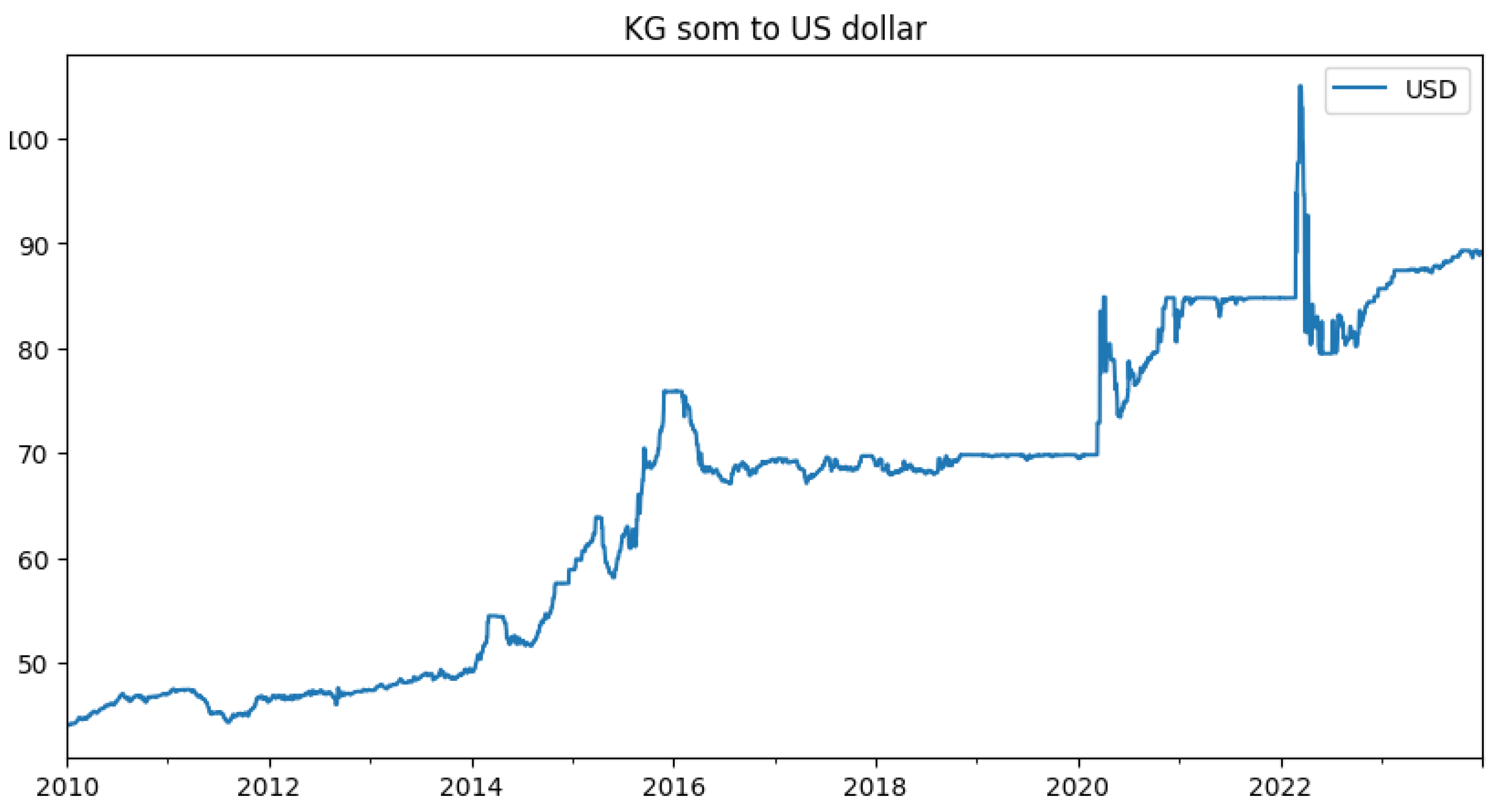
Here is a plot of the volatility of the KG som to US dollar currency pair:
Figure 1.
KG som to US dollar volatility 2010 - 2023
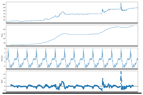
3.1.2. Trend/Seasonal Decomposition
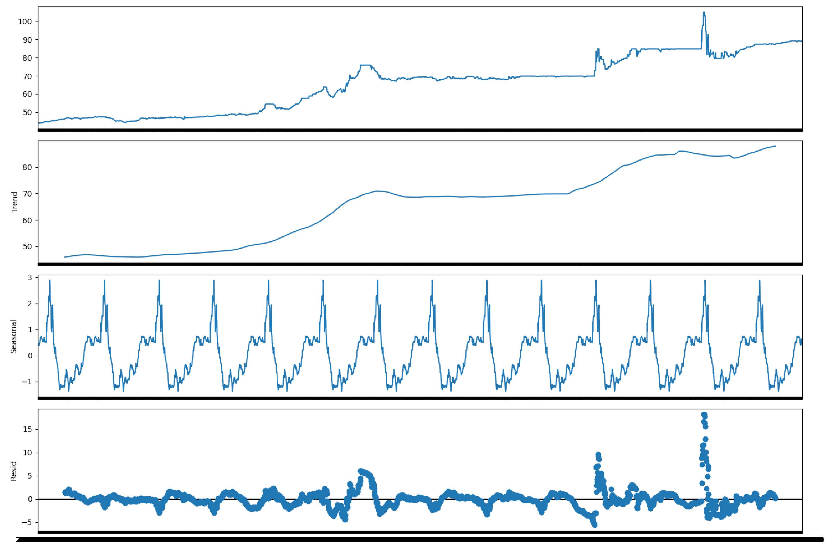
Here is a group of plots after a trend/seasonal decomposition performed on the time series (seasonal_decompose of the statsmodels tool).
Figure 2.
Time series trend/seasonal decomposition
3.2. Stationarity Test
3.2.1. ADF – General Information
In many time series forecasting models, the data should be tested for stationarity before fitting them. Especially if the models are highly dependent on trends and seasonal factors (mostly linear models, such as ARIMA, SARIMA, SARIMAX, VAR) [3] [pp 527-528] [10] [pp 82-84]. In this study, the Augmented Dickey-Fuller (ADF) test was used to test the stationarity of the data before models’ implementation. The ADF-test was imported from the statsmodels library. Here are the results of the test:
- ADF : -0.6919280523080794
- P-Value : 0.8488292899101373
- Num Of Lags : 32
- Num Of Observations Used For ADF Regression and Critical Values Calculation : 5080
-
Critical Values:
- (a)
- – 1% : -3.4316379148442406
- (b)
- – 5% : -2.8621091210661658
- (c)
- – 10% : -2.567072943494637
3.2.2. ADF Interpretation
ADF : -0.6919280523080794 - Critical value of the data according to the ADF-test. P-Value : 0.8488292899101373 - p-value of 0.85>0.05(if we take 5% significance level or 95% confidence interval), null hypothesis (the time series is non-stationary according to ADF) cannot be rejected. Since critical value -0.69>-3.43,-2.86,-2.57 (t-values at 1%,5%and 10% confidence intervals), null hypothesis cannot be rejected. Therefore the dataset is non-stationary
The code with ADF implementation is provided in the Appendix A to the research.
3.3. Prophet Model Instead ARIMA
3.3.1. Prophet Model Explained
Since the data is non-stationary, it should be converted to stationary to implement the ARIMA model (using such techniques, as, for example, differencing). In addition, to obtain reliable and robust model inference, parameters such as order for ARIMA or order and seasonal order for SARIMA/X should be fine-tuned (usning, for example, autocorrelation (ACF/PACF), or mutual information (MI)) [11] [p. 3].
Taking these steps into account, the main limitation of ARIMA methods is the complexity of their implementation. Therefore, it is reasonable to replace them with other methods, such as Prophet and linear regression.
Prophet model: this model was introduced by Facebook (since October 2021 – Meta) in 2017. The model is available in Python and R, and can handle time series data with seasonality, holidays, and trends [10] [p 82].
Prophet can be considered as a nonlinear regression model, of the form:
where:
- g(t) describes a piecewise-linear trend (or “growth term”);
- s(t) describes the various seasonal patterns;
- h(t) captures the holiday effects; and
- is a white noise error term.
3.3.2. Prophet Implementation
Here is a plot with a prediction from the Prophet model:
Figure 3.
Forecast from the Prophet model
The Prophet model was imported from the ETNA library. Using the ETNA library, the data were divided into training and test sets with a forecast horizon of 1 year (horizon = 365 days). Then a Prophet model, imported from ETNA, was fitted and a prediction made for the forecast horizon. Finally, using the mean absolute percentage error (MAPE) and mean absolute error (MAE), the received predicted data were compared to the test set. Comparing to ARIMA models, the Prophet model is simple, and does not require complex preprocessing.
3.4. Exponential Smoothing
3.4.1. About Popular Exponential Smoothing Methods
Exponential smoothing methods are another branch of algorithms used for time series forecasting. Compared to other methods, such as ARIMA, exponential smoothing methods are relatively simple. These methods are particularly successful in short-term forecasting [5][pp 1-2].
There are three most popular exponential smoothing methods: 1) simple exponential smoothing (SES); 2) double exponential smoothing (Holt model); 3) triple exponential smoothing (Holt-Winters model).
3.4.2. Simple Exponential Smoothing
Here is a simple exponential smoothing formula:
In this formula:
- represents the forecast for the next period ;
- represents the actual value at time t;
- represents the forecast for time t;
- is the smoothing parameter, with .
The SES method is considered a naive and weak method that does not take into account any clear trend or seasonality. It only considers the level component (the average value of the series), and uses a single smoothing parameter () to control the weight of the most recent observation in the forecast.
3.4.3. Double Exponential Smoothing (Holt)
Here is a double exponential smoothing formula:
In this formula:
- represents the forecast for h periods ahead at time t;
- represents the level component at time t;
- represents the trend component at time t;
- represents the actual value at time t;
- is the smoothing parameter for the level component, with ;
- is the smoothing parameter for the trend component, with ;
- h is the number of periods ahead for forecasting.
The Holt method is considered as an extension of the SES method. It can successfully handle data with a linear trend, and it updates the level, trend, and seasonal components at each time step. However, this method is unable to capture seasonality. Another weakness of the classical Holt model is the reduction in forecast accuracy when processing data with a damped or exponential trend.
3.4.4. Triple Exponential Smoothing (Holt-Winters)
Here is a triple exponential smoothing formula:
In this formula:
- represents the forecast for h periods ahead at time t;
- represents the level component at time t;
- represents the trend component at time t;
- represents the seasonal component at time t;
- represents the actual value at time t;
- is the smoothing parameter for the level component, with ;
- is the smoothing parameter for the trend component, with ;
- is the smoothing parameter for the seasonal component, with ;
- m represents the number of seasons in a cycle;
- represents the seasonal index for the forecast horizon.
The Holt-Winters method incorporates seasonality in addition to the level and trend components. This method captures repeating patterns in data (seasonal component). Due to the seasonal component, this method is effective in capturing exponential trends (especially the method with multiplicative seasonality). Finally, both the Holt and Holt-Winters methods can be fine-tuned to detect a damped trend.
3.4.5. Exponential Smoothing in this Study
This study uses only the triple exponential smoothing method because this method is able to capture both seasonality and trend [12][p.1515].
Here is a plot with a prediction from the Triple Exponential Smoothing model:
Figure 4.
Forecast from the Holt-Winters model
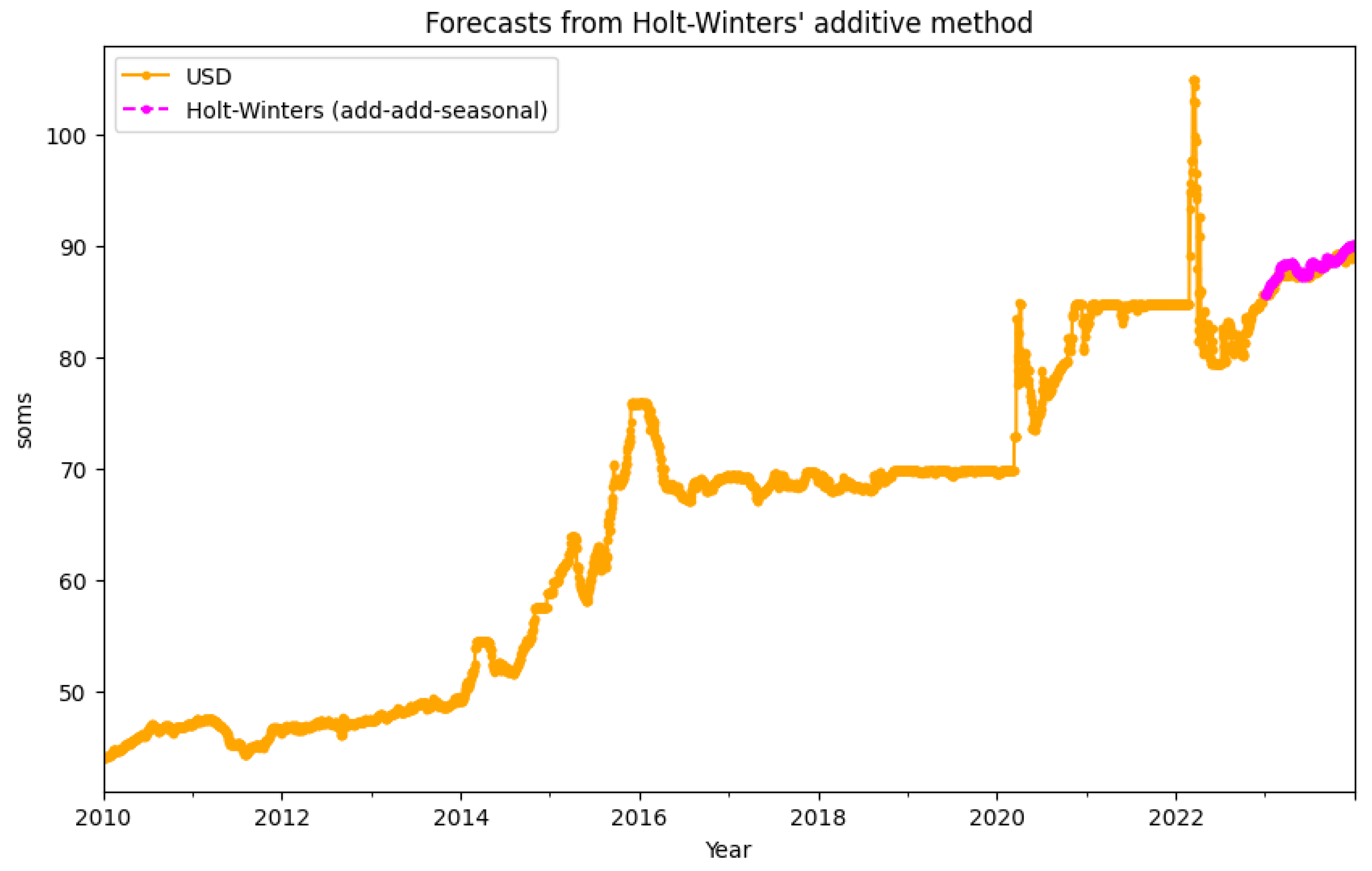
While working on this method, the data were manually divided (using the Python loc() function) into training and test sets. 13 years were allocated for the training set (2010-2022), and 1 year (2023) for the test set. A model of the triple exponential smoothing was taken from the statsmodels Python library, and fitted with following parameters: seasonal periods - 365 (days in a year), trend and seasonality - additive. In addition, the distribution of the data during fitting was normalized using the Box-Cox transformation. Finally, using the mean absolute percentage error (MAPE) and mean absolute error (MAE), the received predicted values were compared to the test set.
3.5. Machine Learning
3.5.1. Preprocessing
This study focuses on supervised ML methods. According to Masini et al., the supervised ML methods can be generally divided in two groups: linear and non-linear methods [6] [p. 2]. Thus, the study examines the performance of two machine learning (ML) algorithms: multiple linear regression (MLR) as an instance of the linear class of methods and decision tree ensembles as an instance of the nonlinear class of methods.
Before building and fitting the models, the data set was divided into training and test sets using a specially created function - data preprocessing with an argument test_size, which splits the data sequentially. So, 80% of the entire dataset, or 4090 rows (up to row index 4090), were placed into the training set (test_size=0.2). In addition, this function was used to add lags and aggregated averages to form a preprocessed dataset.
Lagging a time series means to shift its values forward one or more time steps, or equivalently, to shift the times in its index backward one or more steps. It is worth noting that for better model output, lagged features should be fitted (selected) using different techniques such as ACF/PACF, AIC/BIC, or MI (mutual information). In order to save time and efforts of the researchers, this study skipped the step of selecting better features for lagging. Thus, the Results section of this study presents the results of models fitted with lags selected using the "trial and error" technique. After this, all NaN values that appeared after the lagging process were removed.
Finally, weekday (for each day of the week), monthly and yearly mean values were grouped and added as aggregated features. When grouping aggregated features, only data from the training set were used to avoid data leakage and possible overfitting.
3.5.2. Linear Regression
Linear regression algorithms have been successfully used for time series prediction. This study presents the performance of multiple linear regression (MLR). MLR takes two or more independent variables as predictors, and tries to find relationship between these predictors and a single dependent variable. Here is a general formula of MLR:
In this formula:
- Y - is the dependent variable;
- - are the independent variables;
- - are the coefficients, representing the effect of each independent variable on the dependent variable;
- - is the error term.
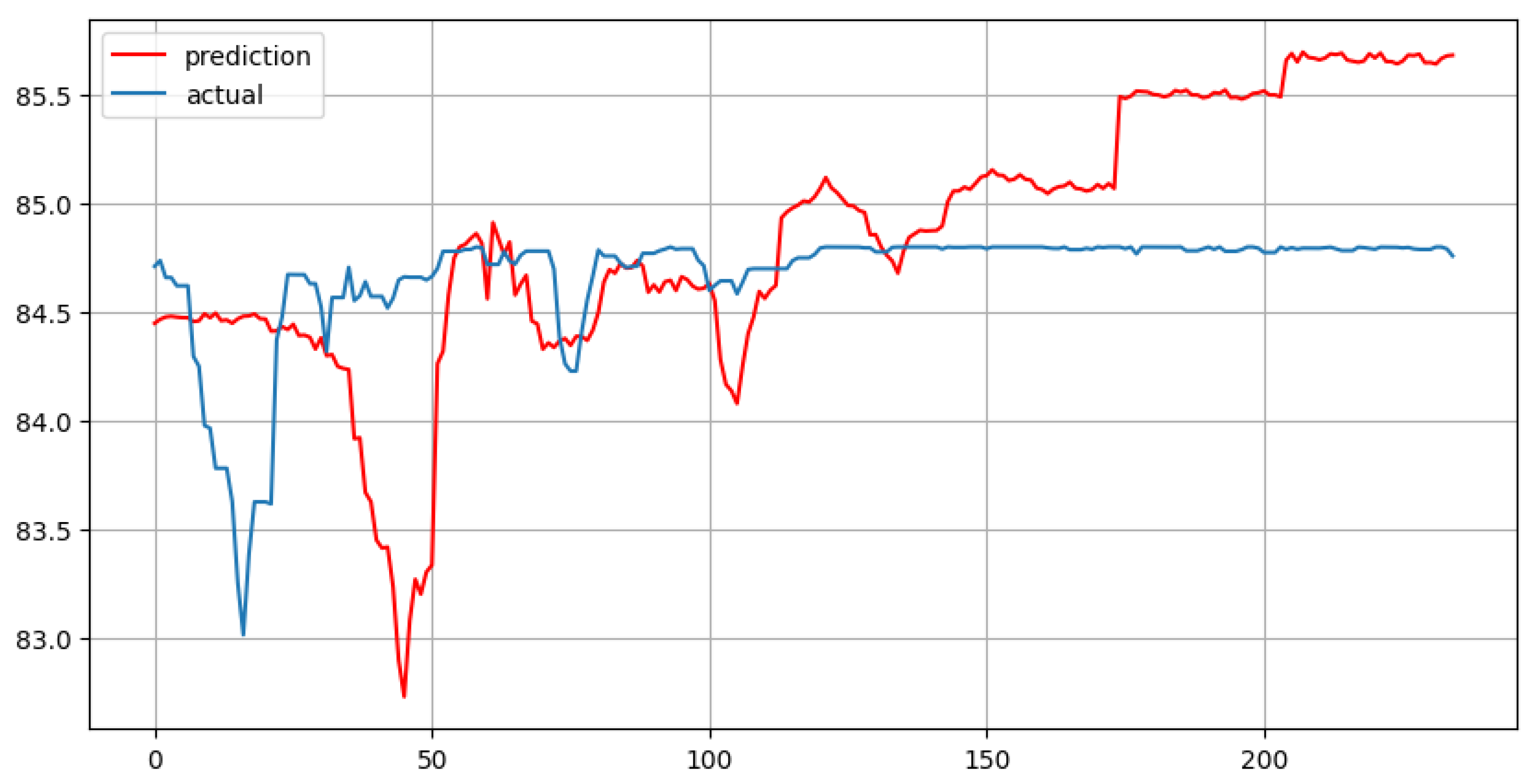
Two groups of lags were used in the MLR implementation process: number of 7 lags (lag_start=7 and lag_end=14) and number of 30 lags (lag_start=29 and lag_end=59) as features (days representing a duration of 1 week and 1 month, respectively). In addition, three more features were added as columns with mean values (weekday, monthly and yearly averages) into each of the two sets. Final sets prepared for fitting an MLR contained 10 (7+3) and 33 (30+3) features, respectively.
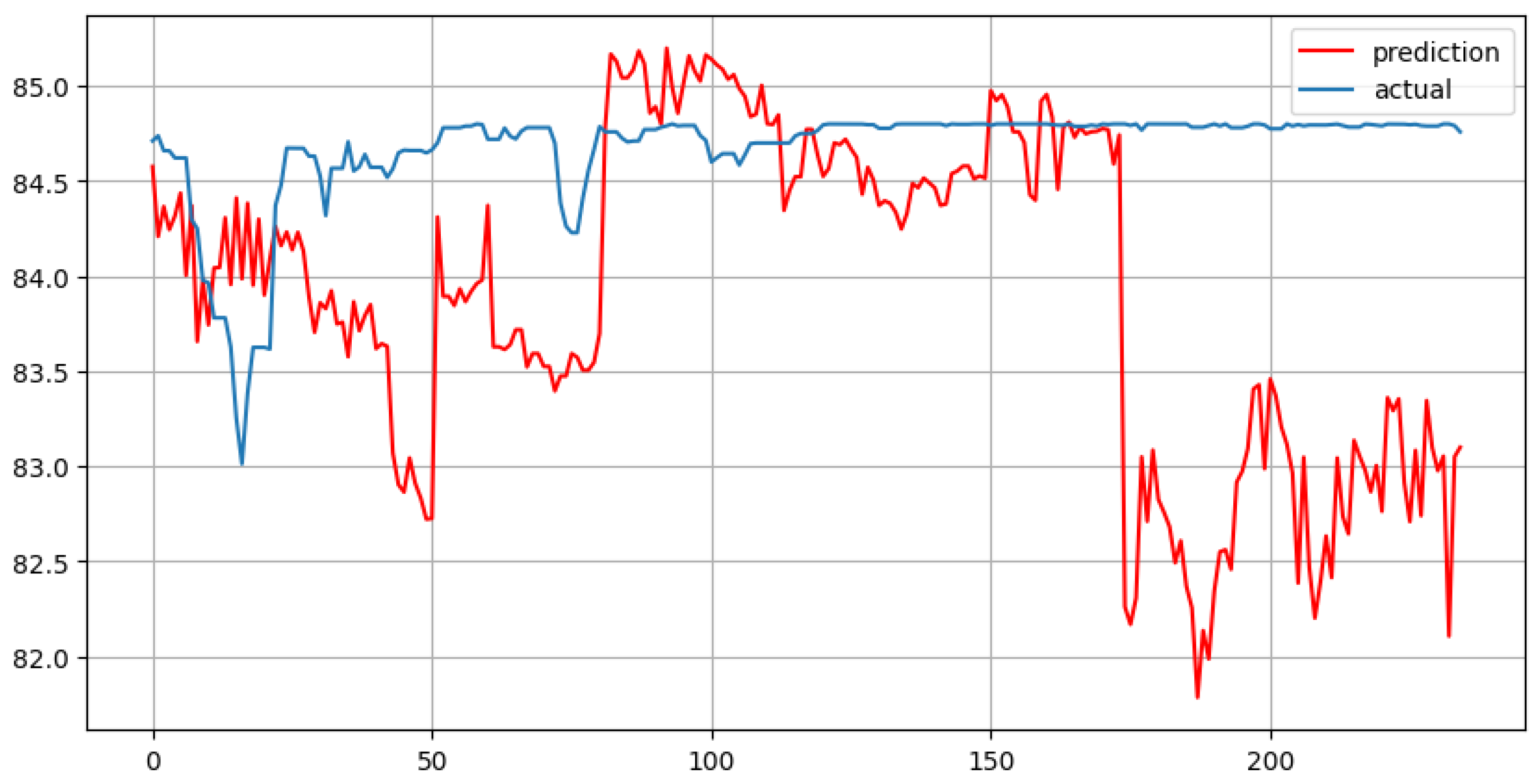
At the next stage, the Linear Regression model, imported from scikitlearn library, was fitted using the training data, and a prediction was made for a horizon of 280 (for the dataset containing 10 features) and 235 (for the dataset containing 33 features) days. The difference between forecast horizons is due to the difference in the creation of lags, as well as the logic of the data_preprocess function (see the code in the research Appendix A).
Figure 5.
Multiple Linear Regression with 7 lags and forecast horizon of 280 days
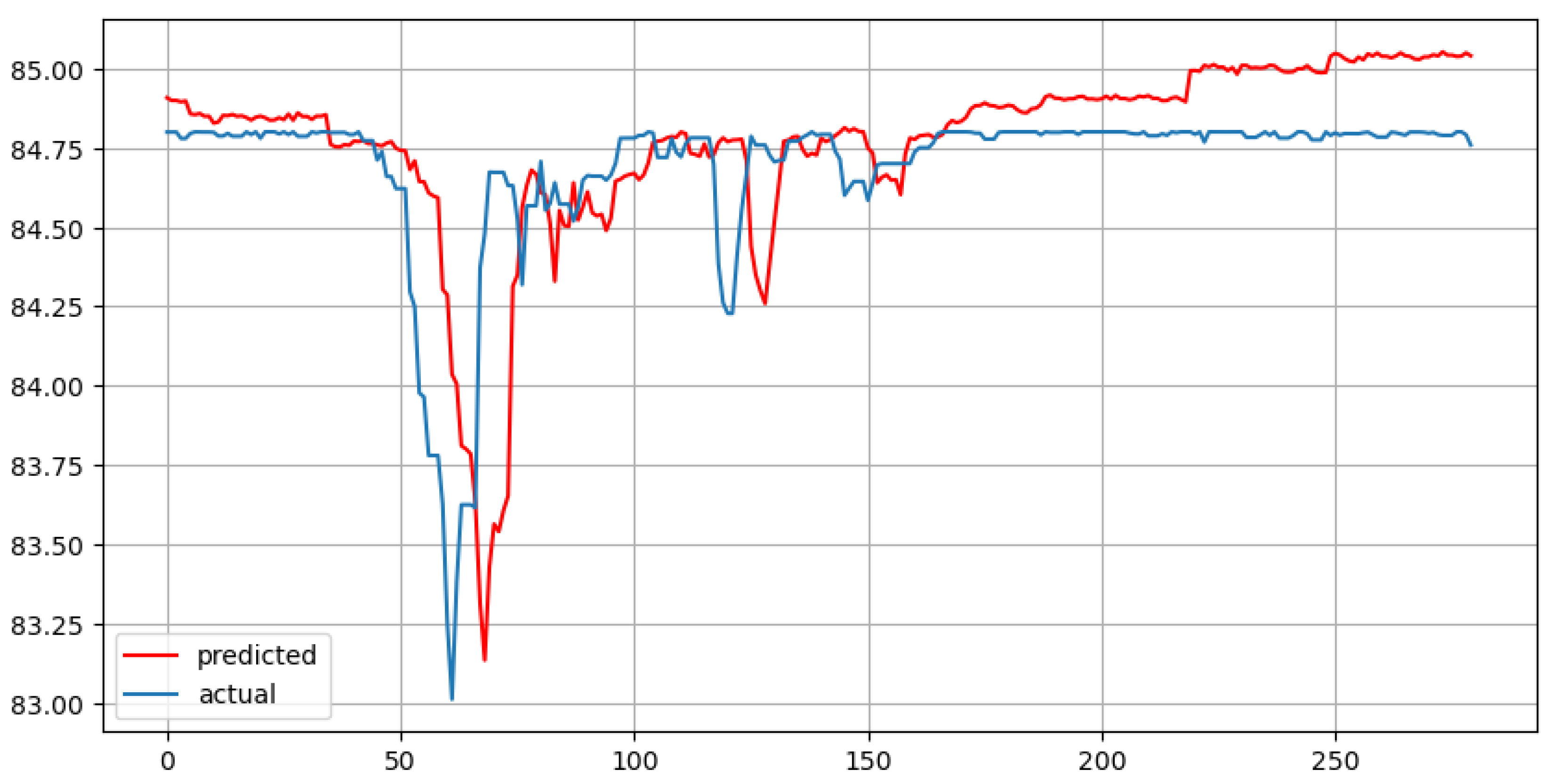
Figure 6.
Multiple Linear Regression with 30 lags and forecast horizon of 235 days
3.5.3. Overfit of MLR
Looking at the charts above, it should be noted that both MLR models (with 7 and 30 lag features) are likely to present overfitting. MLR deals with multiple independent variables. Therefore, quite often researchers can observe the phenomenon of multicollinearity (strong correlation) between independent features, especially when using lags.
The VIF is a standard technique for detecting and quantifying multicollinearity [13] [p. 1]. As a rule of thumb, a VIF greater than 5000 means that independent variables are highly correlated. According to the results provided in the both tables above, all the lag features are significantly (more than 10000) correlated. That means that the model is prone to overfitting. To avoid such a situation, the MLR model should be penalized, using one of the following techniques: LASSO or ridge regression, or their combination called Elastic Net [6] [pp 4-6].
Here are two tables (for 10 features and for 33 features) with results on the VIF (variance inflation factor) metric:

Table 1.
VIF on dataset with 7 lags
| No. | feature | VIF |
|---|---|---|
| 0 | lag_7 | 48246.3 |
| 1 | lag_8 | 101696.7 |
| 2 | lag_9 | 101732.8 |
| 3 | lag_10 | 100864.0 |
| 4 | lag_11 | 101666.9 |
| 5 | lag_12 | 101559.6 |
| 6 | lag_13 | 48088.3 |
| 7 | weekday_avg | 3716.3 |
| 8 | month_avg | 3707.3 |
| 9 | year_avg | 739.7 |
Table 2.
VIF on dataset with 30 lags
| No. | feature | VIF |
|---|---|---|
| 0 | lag_29 | 53463.2 |
| 1 | lag_30 | 115981.8 |
| 2 | lag_31 | 116458.5 |
| 3 | lag_32 | 117514.1 |
| 4 | lag_33 | 119585.7 |
| 5 | lag_34 | 119619.6 |
| 6 | lag_35 | 118806.4 |
| 7 | lag_36 | 118357.1 |
| 8 | lag_37 | 118252.4 |
| 9 | lag_38 | 116112.4 |
| 10 | lag_39 | 114195.0 |
| 11 | lag_40 | 115384.8 |
| 12 | lag_41 | 115613.3 |
| 13 | lag_42 | 115651.6 |
| 14 | lag_43 | 115478.3 |
| 15 | lag_44 | 115439.0 |
| 16 | lag_45 | 115534.6 |
| 17 | lag_46 | 115417.0 |
| 18 | lag_47 | 115109.5 |
| 19 | lag_48 | 113850.2 |
| 20 | lag_49 | 115684.6 |
| 21 | lag_50 | 117737.2 |
| 22 | lag_51 | 117760.6 |
| 23 | lag_52 | 118130.2 |
| 24 | lag_53 | 118858.3 |
| 25 | lag_54 | 118742.7 |
| 26 | lag_55 | 116604.2 |
| 27 | lag_56 | 115483.5 |
| 28 | lag_57 | 114932.2 |
| 29 | lag_58 | 52856.5 |
| 30 | weekday_avg | 3601.7 |
| 31 | month_avg | 3590.7 |
| 32 | year_avg | 814.1 |
Another way to deal with the problem of multicollinearity (high correlation between independent variables) in linear models is through careful feature selection and feature engineering. For example, other values could be selected for the lagging (using such tools, as ACF/PACF or AIC/BIC). Other exogenous factors (e.g., other currencies or some macroeconomic indicators and parameters) could be added as features to improve robustness of the model. Thus, the MLR model would provide more reliable results than those presented.
3.5.4. Decision Tree Ensembles
Decision trees are good examples of a branch of nonlinear supervised ML methods. The main advantage of these methods is that they are intuitive and easy to interpret. However, these algorithms are prone to overfitting, so ensembles of decision trees (bagging or boosting methods) are usually used to solve that problem [6] [pp 19-22].
This study examines the performance of two decision tree algorithms: Random Forest (RF) as an example of bagging ensembles and Catboost as an example of boosting ensembles. The first algorithm was chosen because of its popularity, the second because of its relatively better performance compared to other boosting methods on some benchmarks and metrics [Catboost].
To build the models, the same training and test sets were used (test_size=0.2) as for the MLR. Also, two groups of lags were used as features as in the MLR: number of lags = 7 + 3 aggregated mean features (lag_start=7, lag_end=14) and number of lags = 30 + 3 aggregated features (lag_start=29, lag_end=59).
At the next stage, the Random Forest Regressor (imported from scikitlearn library) and the CatBoost Regressor (imported from catboost library), were fitted using the training data, and a prediction was made for a horizon of 280 (for the dataset containing 10 features) and 235 (for the dataset containing 33 features) days. To make the RF models robust for evaluation, the number of trees is set to 1000 (n_estimators=1000) and the random state is set to 42 (np.random.seed(42), random_state=42). The best number of trees for the CatBoost models using trial and error is 165 (n_estimators=165). In both cases Regressors are used because the purpose of the model is to predict continuous variables (KG som to US dollar daily currency exchange rate). The difference between forecast horizons is due to the difference in the logic of processing lags, as well as the logic of the data_preprocess function (see the code in the research Appendix A).
3.5.5. Selecting Parameters for Decision Tree Ensembles
Choosing the right values of hyperparameters (max_depth, n_estimators, max_features, etc) plays a huge role in the effectiveness of decision tree algorithms. Considering this, the study used a hyperparameter selection method called Random Search Cross-Validation (RSCV), to find best hyperparameters for the models. Surprisingly, the models with default hyperparameter values performed better than the models with values selected with RSCV. One possible reason for this is that RSCV performs a random grid search of proposed hyperparameter options. In addition, it should be taken into account that these results were obtained with the test_size=0.2 (80% of the entire dataset is used as a training set). In case the size of the training set is different, the RSCV provides other values of hyperparameters. Implementation results and comparison of accuracy of different models (basic models with default hyperparameters and models with hyperparameters selected with RSCV; number of features = 3 (no lags added), number of features = 10, and number of features = 33 - only for the CatBoost algorithm) for both algorithms, Random Forest and CatBoost, are provided in the Appendix A part of the research.
3.5.6. Random Forest and CatBoost Charts
Figure 7.
Random Forest with 7 lags and forecast horizon of 280 days
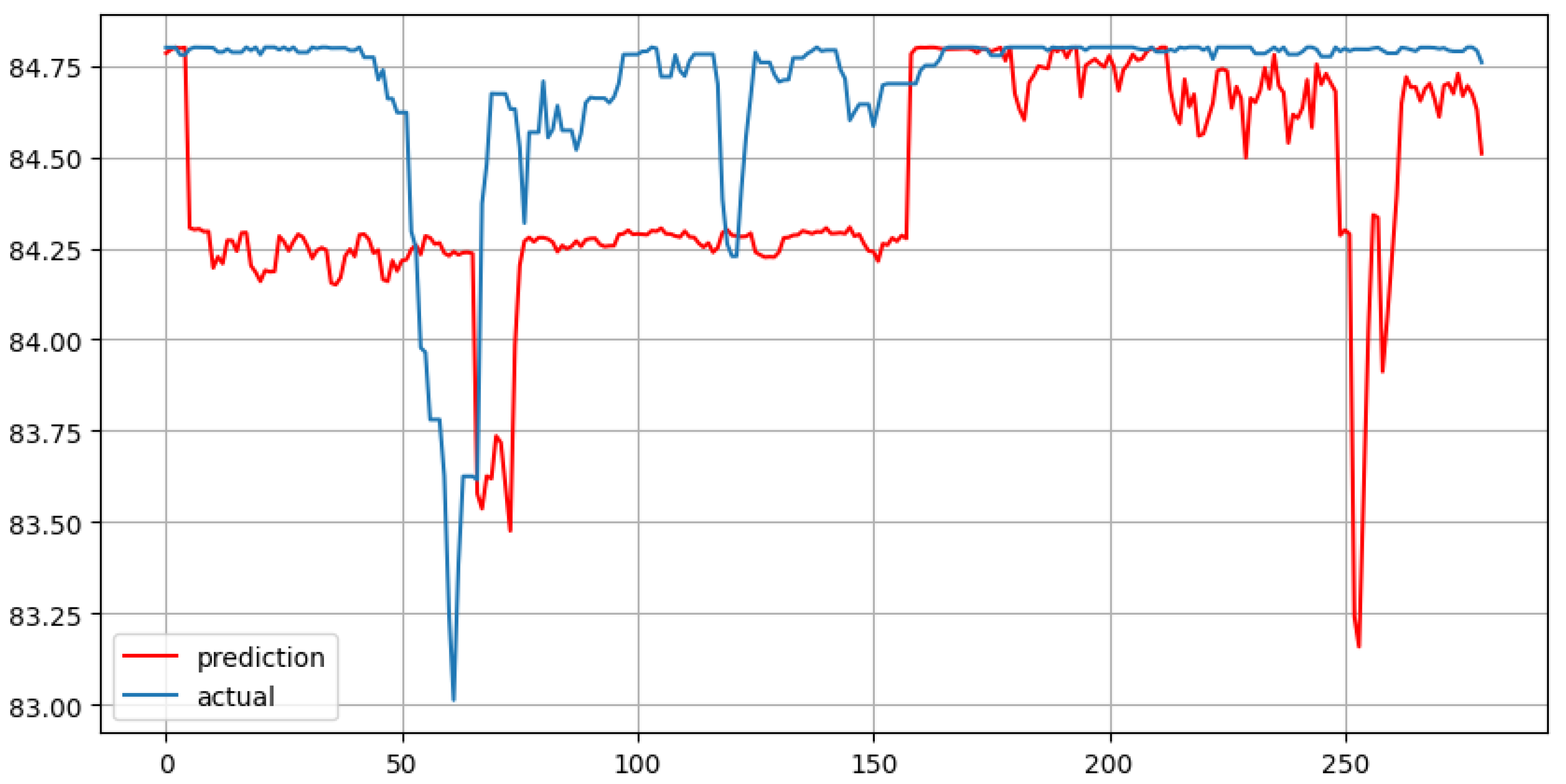
Figure 8.
Random Forest with 30 lags and forecast horizon of 235 days
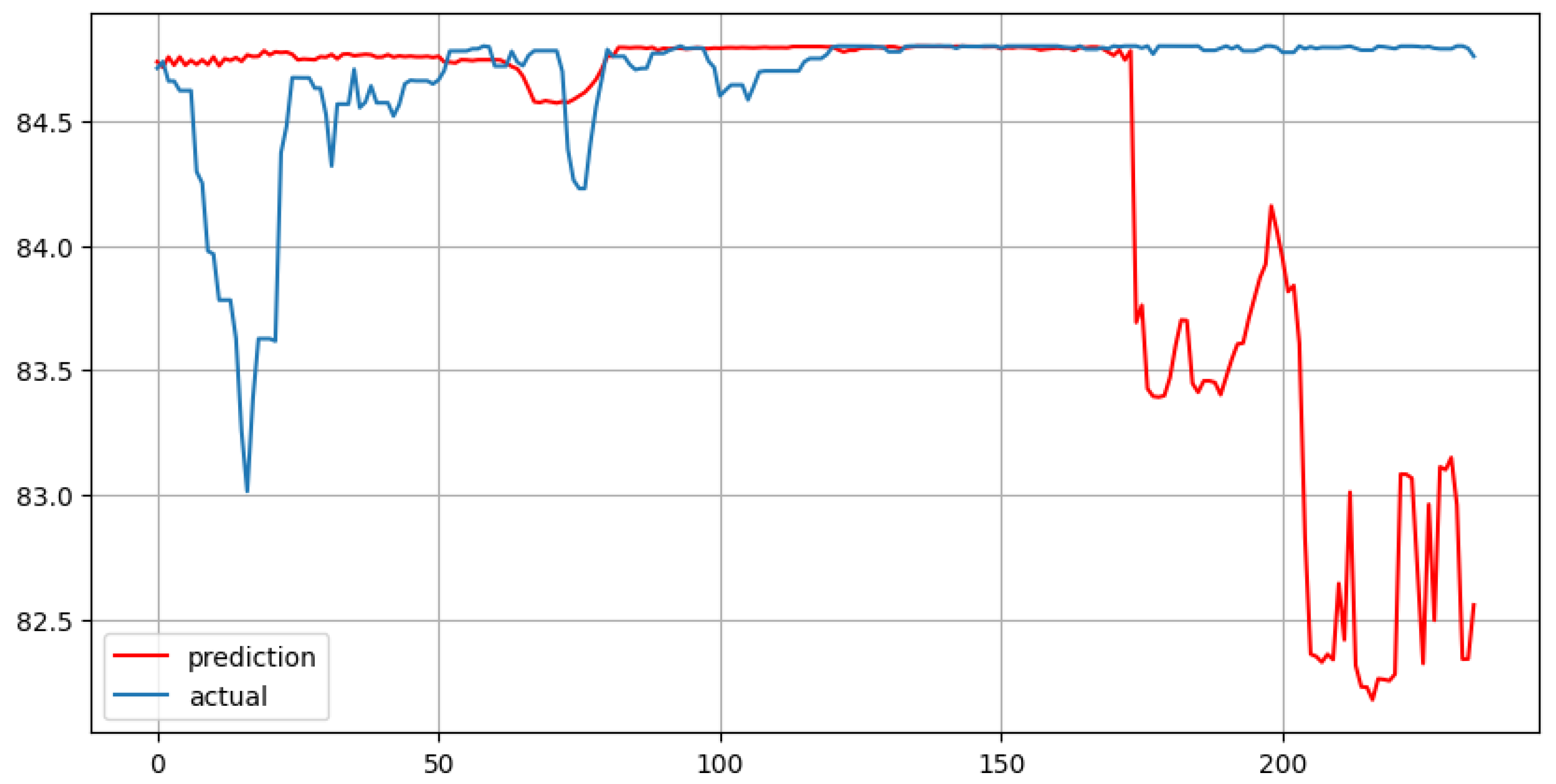
Figure 9.
CatBoost with 7 lags and forecast horizon of 280 days
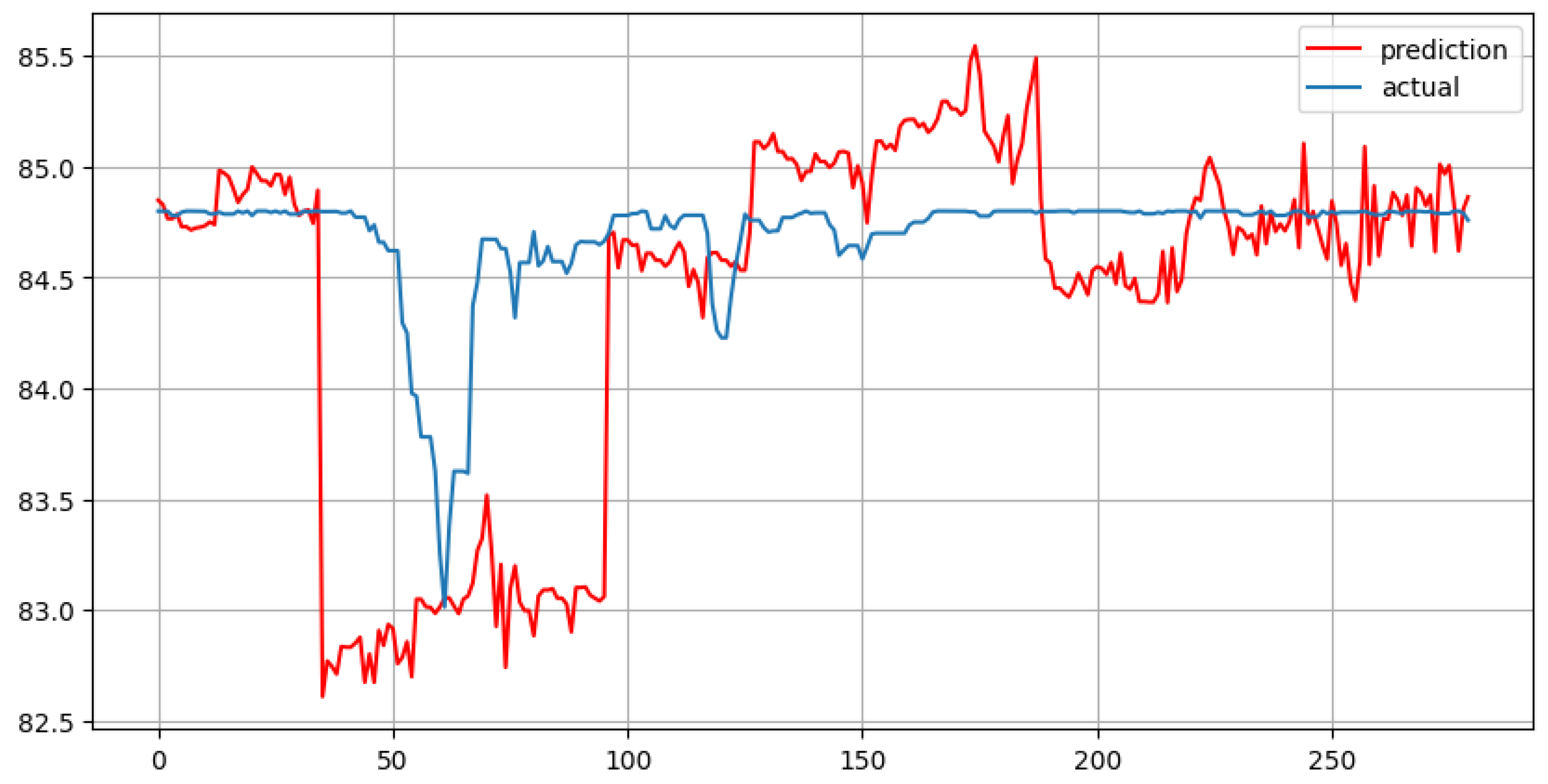
Figure 10.
CatBoost with 30 lags and forecast horizon of 235 days
4. Results and Conclusion
4.1. Table of Results
| Methods’ performance according to metrics | ||
| Method name | MAE | MAPE |
| Prophet | 1.377 | 0.016 |
| Holt-Winters | 0.501 | 0.006 |
| MLR (7 lags) | 0.177 | 0.002 |
| MLR (30 lags) | 0.458 | 0.005 |
| RF (7 lags) | 0.332 | 0.004 |
| RF (30 lags) | 0.558 | 0.007 |
| CatBoost (7 lags) | 0.487 | 0.006 |
| CatBoost (30 lags) | 0.897 | 0.011 |
4.2. MAE and MAPE
The Mean Absolute Error (MAE) is defined as:
where is the actual value, is the predicted value, and n is the number of observations.
——————————————————————–
The Mean Absolute Percentage Error (MAPE) is defined as:
where is the actual value, is the predicted value, and n is the number of observations.
In general, both metrics calculate errors – the difference between the actual values and the values predicted by models. Thus, the lower the MAE and MAPE, the better the model performs.
4.3. Interpretation of Results
According to the Results Table, the best model among all presented in this study is MLR with 7 lags. It demonstrates the lowest MAE and MAPE scores. However, after analyzing VIF results, it should be noted that MLR with 7 lags is prone to overfitting.
As expected, the highest MAE and MAPE scores were obtained for the Prophet model. Holt-Winters, MLR with 30 lags, Random Forest with 30 lags, CatBoost with 7 lags are in the middle with MAE and MAPE around 0.5 and 0.006 respectively.
One interesting detail is that all the machine learning models presented in this study perform better when the number of lag features is lower. Handling multiple lags is not always better, and careful selection of lag features should be performed to obtain better and more robust model results.
4.4. Discussions and Conclusion
Several areas that can be discussed and explored in future research:
- Prophet model is naive and provides relatively worse results. It makes sense to test ARIMA models instead of Prophet [3].
- The Holt-Winters model with other parameters can be tested in the future. Other exponential smoothing methods or models from specialized tools can be used to obtain more accurate and reliable results.
- Lag features for machine learning models can be selected accurately. Model hyperparameters (especially for decision tree ensembles) should be properly tuned. Other machine learning algorithms can be implemented for obtaining better results.
- In this study, lags and aggregated averages were used to fit the models. However, it is reasonable to explore the influence of external factors, including geopolitical events, economic policies, regional economic integration, and other global trends. These factors can be measured and added as features for modelling.
- Finally, this study does not explore the broad scope of using deep learning for time series forecasting. Neural network architectures such as RNNs perform relatively well in time series forecasting tasks. Thus, the use of LSTM or GRU along with performance evaluation using other sophisticated metrics can be considered as the right direction to expand this area of research [4] [8].
The research is not ideal and needs to be supplemented and restructured. As it is stated in the introductory chapter to the paper, the main objective of this study is to compare the performance of several time series models in predicting the volatility of the Kyrgyz som exchange rate against the US dollar. More significant, however, is the implicit idea presented in the abstract of this work - to open up this area to local and international research.
Appendix A. Trend/Seasonal Decomposition
- from statsmodels.tsa.seasonal import
- seasonal_decompose
- decompose_data = seasonal_decompose(data,
- period=365, model="multiplicative")
- decompose_data.plot()
- data – the dataset;
- period = 365 – because the decomposition is made on the period of 1 year (365 elements/days);
- Both models, additive and multiplicative, are tested. There are no significant changes in the plots of both models. Therefore, this attribute change is optional.
Appendix A.1. ADF-Test
- from statsmodels.tsa.stattools import adfuller
- dftest = adfuller(data.USD, autolag = ’AIC’)
- print("1. ADF : ",dftest[0])
- print("2. P-Value : ", dftest[1])
- print("3. Num Of Lags : ", dftest[2])
- print("4. Num Of Observations Used For
- ADF Regression and Critical Values
- Calculation :", dftest[3])
- print("5. Critical Values :")
- for key, val in dftest[4].items():
- print("\t",key, ": ", val)
- data.USD – the USD column of the dataset;
- autolag – according the documentation to the statsmodels tool, this method automatically determines the lag length in the range 0, 1. AIC is a default method.
Appendix A.2. Prophet Model
- from etna.models import ProphetModel
- from etna.metrics import MAE, MAPE
- HORIZON=365
- modelProphet=ProphetModel()
- modelProphet.fit(train_ts)
- future_ts=train_ts.make_future(HORIZON)
- forecast_ts=modelProphet.forecast(future_ts)
- The Prophet model for this study is taken from the ETNA library. Therefore, transformations from the original dataset to a TS dataset object and other transformations must be performed before implementing the Prophet model from ETNA.
- In addition, formulas of some metrics in ETNA differ from the original ones. For example, the MAPE formula in ETNA is different from the MAPE formula in sklearn. So, the MAPE for the Results chapter of this study is obtained by dividing the MAPE from ETNA (1.5645) by 100 and rounding.
Appendix A.3. Holt-Winters Model
- from sklearn.metrics import mean_absolute_error,
- mean_absolute_percentage_error
- from statsmodels.tsa.api import
- ExponentialSmoothing
- fit_HW_add = ExponentialSmoothing(
- train_df,
- seasonal_periods=365,
- trend="add",
- seasonal="add",
- use_boxcox=True,
- initialization_method="heuristic",
- ).fit()
- fcast_HW_add = fit_HW_add.forecast(365)
- trend and seasonal components are additive, seasonal_ periods = 365 due to the fact that the model should forecast daily numbers rather than monthly (12), or quarterly averages (4).
- during the study several popular initialization methods from the statsmodels were tested: "heuristic", "legacy-heuristic", "None", "known", and "estimated". The plot and metric values presented in this study are built using a “heuristic” initialization method.
- Other initialization methods with explanations, as well as multiplicative and mixed trend/seasonal components, will be presented in future studies.
- use_boxcox=True – with this attribute the values in the data were normalized, forecast is made for 365 days.
Appendix A.4. Preprocessing for ML Algorithms
- def code_mean(data, cat_feature, real_feature):
- return dict(data.groupby(cat_feature
- [real_feature].mean())
- This function is used to aggregate mean values. In the following step, it will aggregate and provide averages.
- Listing 1. preprocess_data function
- #This function does many different things
- def preprocess_data(data, lag_start=1,
- lag_end=101, test_size=0.1):
- data=pd.DataFrame(data.copy())
- #here we count an index in our df from which
- #we start our test segment
- test_index=int(len(data) * (1 - test_size))
- #here we add lags of the initial Series as features
- for i in range(lag_start, lag_end):
- data[f’lag_{i}’]=data.USD.shift(i)
- #here we create 3 new columns, using these ad-hoc
- #created columns and the code_mean() function (at
- #the next step), we can get average weekday,
- #monthly, yearly values.
- data[’weekday’]=data.index.weekday
- data[’month’]=data.index.month
- data[’year’]=data.index.year
- #here we count average values only on a training
- #part,in order to avoid data leakage
- data[’weekday_avg’]=list(map(code_mean(data
- [:test_index], ’weekday’, ’USD’).get,
- data.weekday))
- data[’month_avg’]=list(map(code_mean(data
- [:test_index], ’month’, ’USD’).get, data.month))
- data[’year_avg’]=list(map(code_mean(data
- [:test_index], ’year’, ’USD’).get, data.year))
- #here we remove the ad-hoc created features,
- #and drop NA values
- data.drop([’weekday’, ’month’, ’year’],
- axis=1, inplace=True)
- data=data.dropna()
- data = data.reset_index(drop=True)
- #here we split our dataset into training and
- #test sets
- X_train=data.loc[:test_index].drop([’USD’],
- axis=1)
- y_train=data.loc[:test_index][’USD’]
- X_test=data.loc[test_index:].drop([’USD’],
- axis=1)
- y_test=data.loc[test_index:][’USD’]
- return X_train, X_test, y_train, y_test
- In the step, using the preprocess_data function, the dataset (df) is divided into training and test sets and lag features are created.
- X_train, X_test, y_train, y_test = preprocess_data
- (df, test_size=0.2, lag_start=7, lag_end=14)
- X_train, X_test, y_train, y_test = preprocess_data
- (df, test_size=0.2, lag_start=29, lag_end=59)
Appendix A.5. MLR and VIF
- Listing 2. MLR
- from sklearn.metrics import mean_absolute_error,
- mean_absolute_percentage_error
- from sklearn.linear_model import LinearRegression
- linReg=LinearRegression()
- linReg.fit(X_train, y_train)
- preds=linReg.predict(X_test)
- Listing 3. VIF
- from statsmodels.stats.outliers_influence
- import variance_inflation_factor
- #the independent variables set - only on X_train
- vif_df = pd.DataFrame()
- vif_df["feature"] = X_train.columns
- #calculating VIF for each feature
- vif_df["VIF"] = [variance_inflation_factor
- (X_train.values, i) for i in range(len
- (X_train.columns))]
Appendix A.6. Random Forest and CatBoost
- Listing 4. Random Forest
- from sklearn.ensemble import RandomForestRegressor
- np.random.seed=42
- rf=RandomForestRegressor(n_estimators=1000,
- random_state=42)
- rf.fit(X_train, y_train)
- preds=rf.predict(X_test)
- Listing 5. CatBoost
- from catboost import CatBoostRegressor
- cb=CatBoostRegressor(n_estimators=165)
- cb.fit(X_train, y_train)
- preds=cb.predict(X_test)
Appendix A.7. Random Search Cross-Validation
- Random Search Cross-Validation (RSCV) is a technique for defining best hyperparameters for the Decision Tree ensembles.
- At the first step, a grid of hyperparameter ranges is initialized.
- At the second step, the method randomly samples from the grid, performing K-fold cross-validation with each combination of values.
- This section provides codes and results for the models with 10 features (7 lags). The results for the models with 3 features (only averages) show that the base models (with default hyperparameters) perform better than the ones selected with RSCV.
- RSCV for Random Forest is time-consuming, so testing 33-feature models is skipped in this study.
- The following function evaluates the effectiveness of both models, Random Forest and Catboost.
- Listing 6. RSCV and base model evaluation
- def evaluate(model, test_features, test_labels):
- predictions = model.predict(test_features)
- errors = abs(predictions - test_labels)
- mape = 100 * np.mean(errors / test_labels)
- accuracy = 100 - mape
- print(’Average Error: {:0.4f}
- degrees.’.format(np.mean(errors)))
- print(’Accuracy = {:0.2f}%.’.format(accuracy))
- return accuracy
Appendix A.7.1. RSCV for Random Forest – Step 1
- #Create a random_grid - propose our model to select
- #the best h_parameters by random walk on the grid
- from sklearn.model_selection import
- RandomizedSearchCV
- #Number of trees in random forest
- n_estimators = [int(x) for x in np.linspace
- (start = 200, stop = 2000, num = 10)]
- # Number of features to consider at every split
- max_features = [’auto’, ’sqrt’]
- # Maximum number of levels in tree
- max_depth = [int(x) for x in np.linspace(10, 110,
- num = 11)]
- max_depth.append(None)
- #Minimum number of samples required to split a node
- min_samples_split = [2, 5, 10]
- #Minimum number of samples required at each leaf node
- min_samples_leaf = [1, 2, 4]
- #Method of selecting samples for training each tree
- bootstrap = [True, False]
- # Create the random grid
- random_grid = {’n_estimators’: n_estimators,
- ’max_features’: max_features,
- ’max_depth’: max_depth,
- ’min_samples_split’: min_samples_split,
- ’min_samples_leaf’: min_samples_leaf,
- ’bootstrap’: bootstrap
- }
- pprint(random_grid)
- {’bootstrap’: [True, False],
- ’max_depth’: [10, 20, 30, 40, 50, 60, 70, 80,
- 90, 100, None],
- ’max_features’: [’auto’, ’sqrt’],
- ’min_samples_leaf’: [1, 2, 4],
- ’min_samples_split’: [2, 5, 10],
- ’n_estimators’: [200, 400, 600, 800, 1000, 1200,
- 1400, 1600, 1800, 2000]}
- Listing 7. pprint(random_grid) -- output
- {’bootstrap’: [True, False],
- ’max_depth’: [10, 20, 30, 40, 50, 60, 70, 80,
- 90, 100, 110, None],
- ’max_features’: [’auto’, ’sqrt’],
- ’min_samples_leaf’: [1, 2, 4],
- ’min_samples_split’: [2, 5, 10],
- ’n_estimators’: [200, 400, 600, 800, 1000, 1200,
- 1400, 1600, 1800, 2000]}
- {’bootstrap’: [True, False],
- ’max_depth’: [10, 20, 30, 40, 50, 60, 70, 80,
- 90, 100, None],
- ’max_features’: [’auto’, ’sqrt’],
- ’min_samples_leaf’: [1, 2, 4],
- ’min_samples_split’: [2, 5, 10],
- ’n_estimators’: [200, 400, 600, 800, 1000, 1200,
- 1400, 1600, 1800, 2000]}
Appendix A.7.2. RSCV for Random Forest – Step 2
- #Random Search Training - we use the random_grid
- #to search for best h_parameters
- #First create a raw model to tune
- rf = RandomForestRegressor()
- #Random search of parameters, using 5 fold cross
- #validation, search across 200 different combinations,
- #and use all available cores
- rf_random = RandomizedSearchCV(estimator = rf,
- param_distributions = random_grid, n_iter = 200,
- cv = 5, verbose=2, random_state=42, n_jobs = -1)
- #Fit the random search model
- rf_random.fit(X_train, y_train)
- rf_random.best_params_
- Listing 8. best_params_ -- output
- {’n_estimators’: 800,
- ’min_samples_split’: 10,
- ’min_samples_leaf’: 4,
- ’max_features’: ’sqrt’,
- ’max_depth’: 100,
- ’bootstrap’: True}
- Listing 9. evaluate - base RF model
- base_model = RandomForestRegressor(n_estimators
- = 10, random_state = 42)
- base_model.fit(X_train, y_train)
- base_accuracy = evaluate(base_model,
- X_test, y_test)
- Listing 10.evaluate - RF RSCV model
- best_random = rf_random.best_estimator_
- random_accuracy = evaluate(best_random,
- X_test, y_test)
-
This is an output of the evaluate function for the base model:
- Average Error: 0.3818 degrees.
- Accuracy = 99.55%.
-
This is an output of the evaluate function for the RSCV model:
- Average Error: 0.5367 degrees.
- Accuracy = 99.37%.
- Looking at the accuracy and average errors of both models, it is clear that the base model performs slightly better.
Appendix A.7.3. RSCV for CatBoost
- from sklearn.model_selection import
- RandomizedSearchCV
- from catboost import CatBoostRegressor
- cb=CatBoostRegressor()
- lr = [float(x) for x in np.linspace(start = 0.02,
- stop = 0.5, num = 25)]
- max_dep = [int(x) for x in np.linspace(10, 250,
- num = 25)]
- leaf_reg = [1, 3, 5, 7, 9]
- cb_random_grid = {’learning_rate’: lr, ’depth’:
- max_dep, ’l2_leaf_reg’: leaf_reg}
- cb_random = RandomizedSearchCV(cb,
- param_distributions = cb_random_grid, n_iter = 200,
- cv = 5, verbose=2, random_state=42, n_jobs = -1)
- cb_random.fit(X_train, y_train)
- Listing 11.evaluate - base CB model
- cb_base_model = CatBoostRegressor(n_estimators = 100)
- cb_base_model.fit(X_train, y_train)
- cb_base_accuracy = evaluate(cb_base_model,
- X_test, y_test)
- Listing 12. evaluate - CB RSCV model
- cb_best_random = cb_random.best_estimator_
- cb_random_accuracy = evaluate(cb_best_random,
- X_test, y_test)
-
This is an output of the evaluate function for the base model:
- Average Error: 3.3815 degrees.
- Accuracy = 96.00%.
-
This is an output of the evaluate function for the RSCV model:
- Average Error: 2.4334 degrees.
- Accuracy = 97.12%.
- Looking at the accuracy and average errors of both models, it is clear that the model with RSCV hyperparameters performs slightly better.
- Pool wrapper for X_train, X_test, y_train, y_test is not used because the dependent variables are not categorical.
References
- Lee, E.; Mah, J.S. Industrial Policy, Industrialization and Economic Development of Kyrgyzstan. Asian Social Science 2020, 16(9), 42–53. [Google Scholar] [CrossRef]
- Price, R. Economic Development in Kyrgyzstan. K4D Helpdesk Report, 2018; pp. 1 – 26. [Google Scholar]
- Aditya Satrio, C.B.; Darmawan, W.; Nadia, B.U.; Hanafiah, N. Time series analysis and forecasting of coronavirus disease in Indonesia using ARIMA model and PROPHET. Procedia Computer Science 2021, 179, 524–532, 5th International Conference on Computer Science and Computational Intelligence 2020. [Google Scholar] [CrossRef]
- Siami-Namini, S.; Tavakoli, N.; Siami Namin, A. A Comparison of ARIMA and LSTM in Forecasting Time Series. 2018, pp. 1394–1401. [Google Scholar] [CrossRef]
- Gardner Jr., E. S. Exponential smoothing: The state of the art. Journal of Forecasting 1985, 4, 1–28. [Google Scholar] [CrossRef]
- Masini, R.; Medeiros, M.; Mendes, E. Machine Learning Advances for Time Series Forecasting. 2020. [Google Scholar]
- Ni, L.; Li, Y.; Wang, X.; Zhang, J.; Yu, J.; Qi, C. Forecasting of Forex Time Series Data Based on Deep Learning. Procedia Computer Science 2019, 147, 647–652, 2018 International Conference on ldentification, Information and Knowledge in the Internet of Things. [Google Scholar] [CrossRef]
- Dautel, A.; Härdle, W.K.; Lessmann, S.; Seow, H.V. Forex exchange rate forecasting using deep recurrent neural networks. Digital Finance 2020, 2. [Google Scholar] [CrossRef]
- Yamak, P.T.; Yujian, L.; Gadosey, P.K. A Comparison between ARIMA, LSTM, and GRU for Time Series Forecasting. 2020; p. 49–55. [Google Scholar] [CrossRef]
- Samal, K.K.R.; Babu, K.S.; Das, S.K.; Acharaya, A. Time Series based Air Pollution Forecasting using SARIMA and Prophet Model 2019. p. 49–55; p. 80–85. [Google Scholar] [CrossRef]
- Tlegenova, D. Forecasting Exchange Rates Using Time Series Analysis: The sample of the currency of Kazakhstan. 2015. [Google Scholar]
- Alysha, M. De Livera, R.J.H.; Snyder, R.D. Forecasting Time Series With Complex Seasonal Patterns Using Exponential Smoothing. Journal of the American Statistical Association 2011, 106, 1513–1527. [Google Scholar] [CrossRef]
- Christopher Glen Thompson, Rae Seon Kim, A.M.A.; Becker, B.J. Extracting the Variance Inflation Factor and Other Multicollinearity Diagnostics from Typical Regression Results. Basic and Applied Social Psychology 2017, 39, 81–90. [CrossRef]
Disclaimer/Publisher’s Note: The statements, opinions and data contained in all publications are solely those of the individual author(s) and contributor(s) and not of MDPI and/or the editor(s). MDPI and/or the editor(s) disclaim responsibility for any injury to people or property resulting from any ideas, methods, instructions or products referred to in the content. |
© 2025 by the authors. Licensee MDPI, Basel, Switzerland. This article is an open access article distributed under the terms and conditions of the Creative Commons Attribution (CC BY) license (http://creativecommons.org/licenses/by/4.0/).
Copyright: This open access article is published under a Creative Commons CC BY 4.0 license, which permit the free download, distribution, and reuse, provided that the author and preprint are cited in any reuse.


