
Submitted:
15 January 2025
Posted:
16 January 2025
You are already at the latest version
Abstract
Brain Computer Interface (BCI) technology is recently being spotlighted as the performance of Artificial Intelligence (AI) increased drastically. Although there are several instruments to measure brain's activity, Electroencephalography(EEG) signal is in limelight as it has high temporal resolution and is non-invasive, while being extremely portable. However, the raw EEG signals can not be directly used in BCI systems as it includes a lot of artifacts, and has numerous channels. Therefore, selecting only the needed channels and rejecting ones that include big noises are crucial to increase the performance of classification. Motor Imagery EEG (MI-EEG) is a type of EEG where subjects imagine that they are moving their body. MI-EEG channel selection techniques can be divided into two big groups: Common Spatial Pattern (CSP) based models and non-CSP based models. Therefore in this paper, we introduce the models classified in the criteria above, using detailed and strict mathematical terms, and compare each approach's accuracies.
Keywords:
Electroencephalography
; EEG
; Motor Imagery
; Channel Selection
1. Introduction
Brain Computer Interface(BCI) systems measure the activities of the brain in order to perform specific tasks such as interpreting one’s will to speak or move. While there are numerous methods to measure the brain’s activity, such as EEG (electroencephalography), fMRI (functional magnetic resonance imaging), and MEG (Magnetoencephalography), BCI systems utilizing scalp EEG(henceforth called EEG) is trending as it has high temporal resolution, is non-invasive, and extremely portable.
EEG signals are measured by attaching electrodes on the scalp according to the montage, which is a standardized arrangement of electrodes and selection of channel pairs. Montages are divided into two groups: referential and bipolar, by how channels are formed. In referential montage, the voltage difference between each electrode and one reference electrode is recorded, and forms a channel. In Bipolar montage, the voltage difference among consecutive two electrodes are recorded, and forms a channel. The recorded signals then go through artifact and noise removal process to remove undesired signals.[3]
Then, channel selection reduces the number of channels used in feature extraction and classification and ensures that only meaningful channels are included in the process afterwards. After the channel selection, only the necessary channels’ data are needed to be acquired from subjects, so it can help reduce the time consuming setup process and inconvenience for subjects. Also, reducing the number of channels helps reduce computational complexity and increases classification accuracy. [2] Channel selection usually follows the following Figure 2:
Motor Imagery EEG (MI-EEG) is a measurement of EEG signals while subject simulates its movement without actually moving. Therefore MI-EEG based BCIs have been suggested as a substitute method for control, especially for people who are disabled or suffering from locked-in syndrome.[4] It is widely accepted that imagination of a movement stimulates same neural pathway as real movement[5], and can even lead to muscle growth[6]. Traditional Statistical filters used for MI-EEG analysis can be divided into CSP (Common Spatial pattern)-based and non CSP-based filters.[2] Therefore, this paper will discuss about CSP based, filters and non-CSP based statistical filters used in MI-EEG classification in the following chapters.
2. Common Spatial Pattern(CSP) Based Filters
2.1. Original CSP Filter
The Common Spatial Pattern algorithm is known as a spatial filter effective for EEG filtering by maximizing one class’s variance while minimizing other class’s variance in n orthogonal bases as Figure 3, and can be mathematically induced as follows Derivation.
Derivation[7,8,9]
Let and where C is the number of channels, N is the number of samples per epoch, and T is the number of epochs. represents the t th epoch’s signal. In this paper, only consists of two classes: (class 1) and (class 2) for simplicity. Then normalized covariance matrix of each classes: and is defined as
The covariance matrix is normalized with the sum of the diagonal elements of to remove variances among trials.
- As is symmetric, is symmetric and therefore if we define , it can be orthogonally diagonalized as
- By transforming and back to equation about and , we get
2.2. Filter Bank CSP[10]
Typical frequency band analyzed in MI-EEG is 8-30Hz[11,12]. However, as EEG signals have variance among trials and subjects, algorithms’ performance can be enhanced by selecting specific frequency bands per subjects[13]. Therefore, the authors suggested to divide the frequency bands in small bands(4Hz in this paper), and apply CSP filters to each bands. This technique allowed automatic selection of meaningful frequency bands per subjects.
Although mutual information is not used very common in MI-EEG classification, MIBIF(Mutual Information-based Best Individual Feature) and MIRSR(Mutual Information-based Rough Set Reduction) was used to select features to be trained in this paper, which calculates mutual information among features and selects k features that best represent the data.
2.3. Sparse Common Spatial Pattern (SCSP)
CSP coefficients calculated above, Q, is dense, meaning that most of the entries in the matrix can be considered meaningful, and only some have negligible effect. However, the matrix that includes the selected channels’ coefficients select only some of the columns of Q; therefore the original signal can not be transformed into a shape that can be discriminated clearest. Therefore, the authors have sparsified the CSP spatial filters, which can increase performance as the removed features include relatively unnecessary information compared to original CSP filters.
As CSP algorithm’s projection matrix can be written as
Sparsity of W can be increased with several methods, including norm, norm, and norm, where norm of is defined as
where represents magnitude of vector , making norm the number of non-zero entries of and norm the sum of magnitudes of vectors, also known as Manhattan distance.
According to [15], the norm is more suit as a measure of non-sparsity than and norm as it is bounded within , while and norm does not have an upper bound. Also, norm does not depend on vectors’ size, while and depends on it.
The original CSP algorithm is a complementary case when .
2.4. Robust Sparsd Common Spatial Pattern(RSCSP)
The RSCSP algorithm is a derivative algorithm of the SCSP algorithm developed to reduce the effect of outliers in the EEG signal. The non-robust SCSP algorithm calculates covariance matrix of class i: as (1). As EEG signals are regularized, can be written in the form of
, where and denotes EEG signals of class w concatenated by channels. As outliers can distort covariance matrices, MCD(Minimum Covariance Determinant) is used. MCD can be described as a process to find a subset H of original matrix , such that its determinant is reduced, and can be mathematically represented as an optimization problem of where
when is the breakdown point. FASTMCD algorithm can also be adopted to decrease the complexity of the calculation. FASTMCD algorithm first selects random h points and updates the points by ranking the data by their Mahalanobis distances and select h points with the smallest distances to form a new subset. Then if the new subset has a smaller determinant of covariance matrix, it functions as a new initial set and continues this process until the covariance matrix converges.
3. CSP Based Channel Selection Techniques
3.1. Bhattacharyya Bound of CSP Features
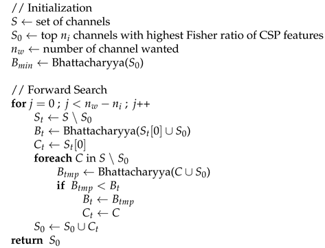
In [7], the authors reduced the number of channels by selecting a set of channels using forward search. Bhattacharyya bound, which is the upper bound of bayes error probability was used as evaluation, as the calculation of Bayes error probability is challenging. The statement: Bhattacharyya bound is the upper bound of Bayes error probability can be proved by Proof.
To summarize, the channels are selected by Algorithm 1
- Proof.
The Bayes error probability can be written as
where and are the prior probabilities of class 1 and 2, respectively. and are are class conditional probability density functions, and x represents an observed data point.
- Sinces ,
| Algorithm 1 Bhattacharyya Bound Based Channel Selection |
 |
3.2. CSP-Rank
CSP-Rank is based on the idea that the matrix in (8) includes the importance of each channel in classification as it acts as a weight to the original signal. The authors of this paper therefore set and selected two vectors: and , where maximizes class i’s variance. Therefore, the channels with the largest entries in each of , , , ⋯ are consecutively selected until the model trained with the selected channels reaches the desired accuracy.
The results are statistically significant at significance compared to random selection. Also, the number of channels needed to reach 90% accuracy was 8-38 channels, while SVM-RFE(Support-vector machine recursive feature elimination, explained in Section 4.1) required 12-28 channels, therefore being better than SVM-RFE.
3.3. Norm of CSP Filter
Since it is widely accepted that the effectiveness of the CSP algorithm decreases as the number of channels increases due to overfitting, the authors first applied the CSP filter to all channels and scored each channel based on its norm. Then, the channels with high scores were selected and used to train the model. The following score is used for calculating channels’ weight:
where is the CSP projection matrix from (8) , and is the ith column of , and can be ordered in decreasing order to select wanted number of channels.
3.4. Cohen’s d Effect Size CSP(E-CSP)
The E-CSP algorithm aims to remove channels that contain redundant information. The algorithm is divided into two major parts: part 1, where the noisy channels are removed, and part 2, where the remaining channels are evaluated to determine if they are meaningful.
First, to remove trials with large artifacts, the z-score calculated by equation, z-score, calculated by (21) is used.
where i, j, l represents channel number, trial,and class, respectively, and is the standard deviation of lth task’s ith channel, is calculated. The z-score was adopted as it measures how far the signal deviates from the average. Therefore, the ith channel’s jth trial can be considered noisy if , where is the criterion of noisy channel. Therefore, let and let the frequency of lth class’ jth trial being noisy as
If the trial’s frequency exceeds the threshold , it is considered as a noisy trial. Therefore, we can define the set of noisy trials as
Therefore, after removing the noisy channels, the ith channel’s mean for jth task can be calculated as
where represents non-noisy channels.
Second, the effect size of channel i is evaluated as a meaningful channel if
where
and stands for the standard deviation of lth class’ ith channel, and represents the criterion for a channel to be thought as meaningless, as the variance among two class is small.
Finally, the leftover channels L, are selected and CSP filter is applied.
4. Non-CSP Based Methods
4.1. Support-Vector Machine Recursive Feature Elimination (SVM-RFE)[21,22]
SVM(Hard Margin Support Vector Machine) Algorithm
Support vector machine is an algorithm that aims to find a hyperplane that maximizes the margin among the given classes. Let there be N data points: where d is the dimension of the point, and be a label. The hyperplane can be written as where w is the weight and b is the bias. The optimization problem of w and b to maximize the margin can be written as
, and this problem can be solved using the Lagrange multiplier.
- Let Lagrange function
Soft Margin SVM Algorithm
SVM-RFE Algorithm
SVM-RFE algorithm aims to find a subset of size r among n variables which maximizes the performance of the classifier using backward sequential selection.
From previous research [22,23], it is well known that can be used as a criterion for elimination. The equation (33) can be transformed into
using Taylor series to the second order. As the objective function J reaches its optimal point, . Therefore,
. When removing ith feature, the weight must be 0, therefore . Therefore, the criterion for removing the ith feature can be approximated as
4.2. Value Based Channel Selection
Similar to how the Bhattacharyya bound-based CSP selection used the F-ratio for selecting the initial subset of channels, the authors of [19] have utilized the value as a control group. is defined as
where , denotes ith channel of , which means , and denotes number of epochs in class k.
4.3. Correlation Based Channel Selection[24,25]
EEG has a limitation that even though one is repeating the same task, due to other activities and thoughts in the brain, different EEG is recorded, and makes it hard to analyze the task performed. The authors assumed that as channels related to MI-EEG while performing same task will contain similar information across trials, thus having high correlation among trials, while channels that are not related will not have alike information, therefore having low correlation.
Pearson’s correlation is used in both papers, which measures linear dependency among random variables, and is calculated by
where are random variables, are means of random variables, and represents standard deviation of X and Y respectively. Correlations are calculated among every channels, forming a correlation matrix of size . By averaging each row, we can find the channel that is most effective. By repeating this procedure among every epochs, we can select number of channels by selecting the channels that are considered to be effective over certain criteria times.
4.4. Genetic Algorithm (GA) Based Selection
Genetic Algorithm(henceforth GA) is a heuristic methodology for finding an optimal solution by mimicking Charles Darwin’s natural evolution theory. Genetic algorithm mimics how genetic information are passed over through generations. Like DNA is formed with genes, a gene is an element that forms a chromosome. A chromosome is a set of genes that forms a potential solution to the problem. The fitness function evaluates how well each chromosome solves the problem. The scores calculated are used for selection, which is a process of selecting chromosomes that will create an offspring. The higher the score is, the higher chance it has to be selected. Like our DNA, an offspring is created by combining the genetic information of two chromosomes. The point where that crossover will be made is randomly selected. For example, aaaa and bbbb can become aaaa, abbb, aabb, abbb,and bbbb. Mutation happens randomly at each position, changing the value from 0 to 1 or 1 to 0.
The genetic algorithm follows the flow chart Figure 4:
Genetic Algorithm For Selecting Optimal Channels for P300 Based Classification [26,27]
EEG signals can be roughly divided into four categories: Visual Evoked Potential (VEP), Sensorimoter Rythm (SRM), Slow Cortical Potentials (SCP), and Event-Related Potentials (ERP). VEP is a signal acquired from three occipital electrodes, while forming two channels by setting the middle electrode as a reference, and represents the pathway of visual activity, from optic nerve to primary optic cortex. SRM is a signal recorded from sensorimotor cortex at mu(7–13 Hz), beta(13–30 Hz), and gamma(30–200 Hz) frequency bands, and is strongly modulated with simple movements and certain cognitive tasks. SCP is a measurement of a slowly changing electrical signal with frequency lower than 1Hz. ERP is not a term referencing an EEG measured in specific location, but is a fluctuation generated by neurons due to some event, such as motor or speech imagery, at a specific time. [26,28,29,30,31,32,33,34].
P300 is an unique ERP, which appears as a positive peak near 300ms after stimulation happens. A 64 channel EEG was recorded and four channels were selected in [26], by defining the fitness function where X is a chromosome consisting four genes, which are channels in this case. is defined as the maximum among four channels, where is a value between 0 and 1, and higher the is, the higher the variance among classes are.
5. Result
In this study, we utilized the EEG dataset from BCI Competition IV Dataset 2a, which is specifically designed for benchmarking motor imagery classification algorithms. The dataset comprises EEG recordings from nine healthy subjects, each performing four different motor imagery tasks: imagining movements of the left hand, right hand, both feet, and tongue. EEG signals were recorded using 22 Ag/AgCl electrodes placed according to the international 10-20 system at a sampling rate of 250Hz [35].
For preprocessing, we applied a band-pass filter between 8Hz and 30Hz, a frequency band commonly used in previous research[11,12]. Baseline correction was performed by subtracting the mean of a 2 second pre-cue interval, mentioned as "Fixation cross" (from -2s to 0s relative to the cue onset), from the subsequent motor imagery data. The entire 4seconds of motor imagery data (from 0s to 4s after the cue onset) were used for classification.
Data were split into training and evaluation datasets using 5-fold cross-validation, ensuring that the classes were balanced in terms of the number of trials in each fold. Cross-validation was performed individually for each subject to account for inter-subject variability of EEG signals.
The accuracies of each algorithm were measured by training a support vector machine (SVM) classifier with a linear kernel using the data from the selected channels.
5.1. CSP and SCSP Algorithm
CSP algorithm can be thought of as a special case of the SCSP algorithm where . The accuracy of SCSP algorithm depends on its r value, so accuracy of SCSP algorithm where is compared as Figure 5.
5.2. Accuracy of CSP Based Channel Selection Methods
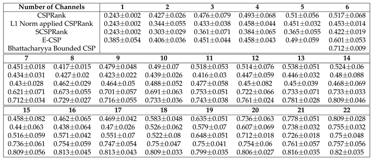
The accuracy of CSP based channel selection methods: CSPRank(Section 3.2), L1 Norm applied CSPRank(Section 3.3), SCSPRank(SCSP used instead of CSP in CSPRank), E-CSP(Section 3.4), and Bhattacharyya bounded CSP(Section 3.1) is as following Table 1 and Figure 6.

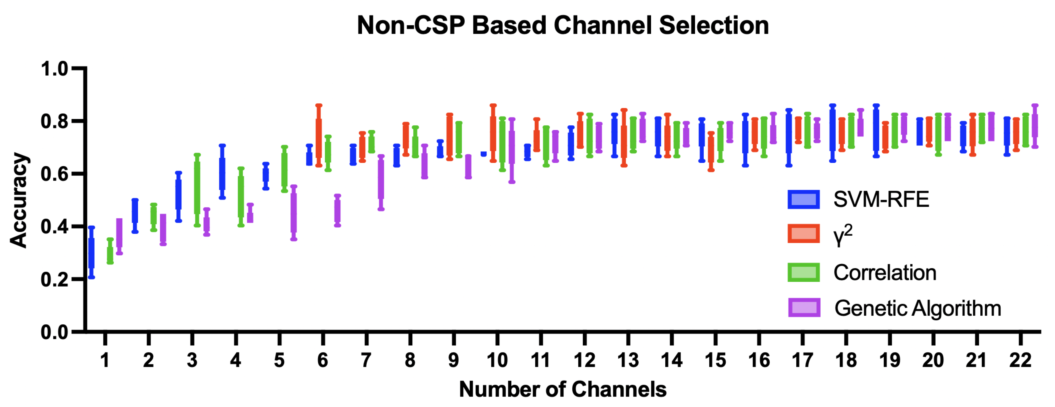
5.3. Accuracy of Non-CSP Based Statistical Channel Selection Methods
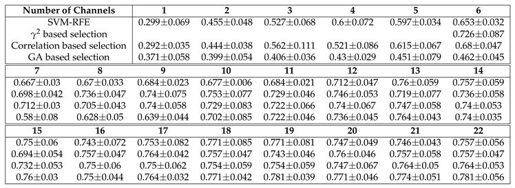
The accuracy of Non-CSP based channel selection methods: SVM-RFE(Section 4.1), value based channel selection(Section 4.2), Correlation based channel selection(Section 4.3), and Genetic Algorithm based channel selection(Section 4.4) is as following Table 2 and Figure 7.
References
- Alotaiby, T.; El-Samie, F.E.A.; Alshebeili, S.A.; Ahmad, I. A review of channel selection algorithms for EEG signal processing. EURASIP Journal on Advances in Signal Processing 2015, 2015, 1–21. [Google Scholar] [CrossRef]
- Baig, M.Z.; Aslam, N.; Shum, H.P. Filtering techniques for channel selection in motor imagery EEG applications: a survey. Artificial intelligence review 2020, 53, 1207–1232. [Google Scholar] [CrossRef]
- Electroencephalography (EEG): An Introductory Text and Atlas of Normal and Abnormal Findings in Adults, Children, and Infants.
- Choi, J.; Kaongoen, N.; Jo, S. Investigation on Effect of Speech Imagery EEG Data Augmentation with Actual Speech. In Proceedings of the 2022 10th International Winter Conference on Brain-Computer Interface (BCI); pp. 1–5. [CrossRef]
- Roth, M.; Decety, J.; Raybaudi, M.; Massarelli, R.; Delon-Martin, C.; Segebarth, C.; Morand, S.; Gemignani, A.; Décorps, M.; Jeannerod, M. Possible involvement of primary motor cortex in mentally simulated movement: a functional magnetic resonance imaging study. NeuroReport 1996, 7. [Google Scholar] [CrossRef] [PubMed]
- Yue, G.; Cole, K.J. Strength increases from the motor program: Comparison of training with maximal voluntary and imagined muscle contractions. Journal of Neurophysiology 1992, 67, 1114–1123. [Google Scholar] [CrossRef] [PubMed]
- Lin, H.; Zhuliang, Y.; Zhenghui, G.; Yuanqing, L. Bhattacharyya bound based channel selection for classification of motor imageries in EEG signals. In Proceedings of the 2009 Chinese Control and Decision Conference; pp. 2353–2356. [CrossRef]
- Ramoser, H.; Müller-Gerking, J.; Pfurtscheller, G. Optimal spatial filtering of single trial EEG during imagined hand movement. IEEE Trans Rehabil Eng 2000, 8, 441–6. [Google Scholar] [CrossRef]
- Fukunaga, K. Chapter 2 - RANDOM VECTORS AND THEIR PROPERTIES. In Introduction to Statistical Pattern Recognition, 2nd ed.; Fukunaga, K., Ed.; Academic Press: Boston, 1990; pp. 11–50. [Google Scholar] [CrossRef]
- Ang, K.K.; Chin, Z.Y.; Wang, C.C.; Guan, C.T.; Zhang, H.H. Filter bank common spatial pattern algorithm on BCI competition IV Datasets 2a and 2b. Frontiers in Neuroscience 2012, 6. [Google Scholar] [CrossRef] [PubMed]
- Blankertz, B.; Tomioka, R.; Lemm, S.; Kawanabe, M.; Muller, K.r. Optimizing Spatial filters for Robust EEG Single-Trial Analysis. IEEE Signal Processing Magazine 2008, 25, 41–56. [Google Scholar] [CrossRef]
- Müller-Gerking, J.; Pfurtscheller, G.; Flyvbjerg, H. Designing optimal spatial filters for single-trial EEG classification in a movement task. Clinical Neurophysiology 1999, 110, 787–798. [Google Scholar] [CrossRef] [PubMed]
- Blankertz, B.; Dornhege, G.; Krauledat, M.; Müller, K.R.; Curio, G. The non-invasive Berlin Brain–Computer Interface: Fast acquisition of effective performance in untrained subjects. NeuroImage 2007, 37, 539–550. [Google Scholar] [CrossRef]
- Arvaneh, M.; Guan, C.; Ang, K.K.; Quek, C. Optimizing the Channel Selection and Classification Accuracy in EEG-Based BCI. IEEE Transactions on Biomedical Engineering 2011, 58, 1865–1873. [Google Scholar] [CrossRef] [PubMed]
- Hurley, N.; Rickard, S. Comparing Measures of Sparsity. IEEE Transactions on Information Theory 2009, 55, 4723–4741. [Google Scholar] [CrossRef]
- Arvaneh, M.; Guan, C.; Ang, K.K.; Quek, C. Robust EEG channel selection across sessions in brain-computer interface involving stroke patients. In Proceedings of the The 2012 International Joint Conference on Neural Networks (IJCNN); pp. 1–6. [CrossRef]
- Duda, R.O.; Hart, P.E.; Stork, D.G. Chapter2 - Bayesian decision theory. In Pattern Classification, 2nd ed.; Duda, R.O., Hart, P.E., Stork, D.G., Eds.; Wiley, 2000; book section 2; pp. 1–32. [Google Scholar]
- Tam, W.K.; Ke, Z.; Tong, K.Y. Performance of common spatial pattern under a smaller set of EEG electrodes in brain-computer interface on chronic stroke patients: A multi-session dataset study. In Proceedings of the 2011 Annual International Conference of the IEEE Engineering in Medicine and Biology Society; pp. 6344–6347. [CrossRef]
- Meng, J.; Liu, G.; Huang, G.; Zhu, X. Automated selecting subset of channels based on CSP in motor imagery brain-computer interface system. In Proceedings of the 2009 IEEE International Conference on Robotics and Biomimetics (ROBIO); pp. 2290–2294. [CrossRef]
- Das, A.K.; Suresh, S. An Effect-Size Based Channel Selection Algorithm for Mental Task Classification in Brain Computer Interface. In Proceedings of the 2015 IEEE International Conference on Systems, Man, and Cybernetics; pp. 3140–3145. [CrossRef]
- Qifeng, Z.; Wencai, H.; Guifang, S.; Weiyou, C. A new SVM-RFE approach towards ranking problem. In Proceedings of the 2009 IEEE International Conference on Intelligent Computing and Intelligent Systems, Vol. 4; pp. 270–273. [CrossRef]
- Guyon, I.; Weston, J.; Barnhill, S.; Vapnik, V. Gene Selection for Cancer Classification using Support Vector Machines. Machine Learning 2002, 46, 389–422. [Google Scholar] [CrossRef]
- LeCun, Y.; Denker, J.; Solla, S. Optimal brain damage. Advances in neural information processing systems 1989, 2. [Google Scholar]
- Jin, J.; Miao, Y.Y.; Daly, I.; Zuo, C.L.; Hu, D.W.; Cichocki, A. Correlation-based channel selection and regularized feature optimization for MI-based BCI. Neural Networks 2019, 118, 262–270. [Google Scholar] [CrossRef] [PubMed]
- Hsu, W.Y.; Cheng, Y.W. EEG-channel-temporal-spectral-attention correlation for motor imagery EEG classification. IEEE Transactions on Neural Systems and Rehabilitation Engineering 2023, 31, 1659–1669. [Google Scholar] [CrossRef] [PubMed]
- Hasan, I.H.; Ramli, A.R.; Ahmad, S.A. Utilization of Genetic Algorithm for Optimal EEG Channel Selection in Brain-Computer Interface Application. In Proceedings of the 2014 4th International Conference on Artificial Intelligence with Applications in Engineering and Technology; pp. 97–102. [CrossRef]
- Kee, C.Y.; Kuppan Chetty, R.M.; Khoo, B.H.; Ponnambalam, S.G. Genetic Algorithm and Bayesian Linear Discriminant Analysis Based Channel Selection Method for P300 BCI. In Proceedings of the Trends in Intelligent Robotics, Automation, and Manufacturing; Ponnambalam, S.G.; Parkkinen, J.; Ramanathan, K.C., Eds. Springer Berlin Heidelberg; pp. 226–235.
- Brenner, R. CHAPTER 77 - INVESTIGATIONS IN MULTIPLE SCLEROSIS. In Neurology and Clinical Neuroscience; Schapira, A.H.V., Byrne, E., DiMauro, S., Frackowiak, R.S.J., Johnson, R.T., Mizuno, Y., Samuels, M.A., Silberstein, S.D., Wszolek, Z.K., Eds.; Mosby: Philadelphia, 2007; pp. 1031–1044. [Google Scholar] [CrossRef]
- Gibson, R.M.; Owen, A.M.; Cruse, D. Chapter 9 - Brain–computer interfaces for patients with disorders of consciousness. In Progress in Brain Research; Coyle, D., Ed.; Elsevier, 2016; Volume 228, pp. 241–291. [Google Scholar] [CrossRef]
- Samar, V.J. Evoked Potentials. In Encyclopedia of Language & Linguistics (Second Edition); Brown, K., Ed.; Elsevier: Oxford, 2006; pp. 326–335. [Google Scholar] [CrossRef]
- Cinzia Baiano, M.Z. Visual Evoked Potential, 2023 May 11.
- Schmidt, S.; Jo, H.G.; Wittmann, M.; Hinterberger, T. ‘Catching the waves’ – slow cortical potentials as moderator of voluntary action. Neuroscience & Biobehavioral Reviews 2016, 68, 639–650. [Google Scholar] [CrossRef]
- Cheyne, D.O. MEG studies of sensorimotor rhythms: A review. Experimental Neurology 2013, 245, 27–39. [Google Scholar] [CrossRef]
- Mudgal, S.K.; Sharma, S.K.; Chaturvedi, J.; Sharma, A. Brain computer interface advancement in neurosciences: Applications and issues. Interdisciplinary Neurosurgery 2020, 20, 100694. [Google Scholar] [CrossRef]
- Tangermann, M.; Müller, K.R.; Aertsen, A.; Birbaumer, N.; Braun, C.; Brunner, C.; Leeb, R.; Mehring, C.; Miller, K.J.; Mueller-Putz, G.; et al. Review of the BCI Competition IV. Frontiers in Neuroscience 6. [CrossRef] [PubMed]
Figure 1.
Procedure of EEG Classification

Figure 2.
Procedure of Channel Selection
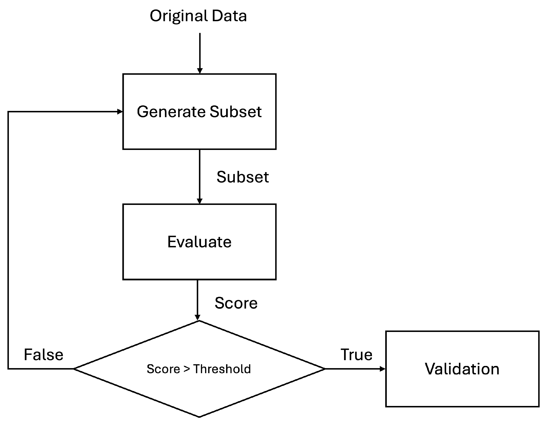
Figure 3.
Example of CSP filtering ()
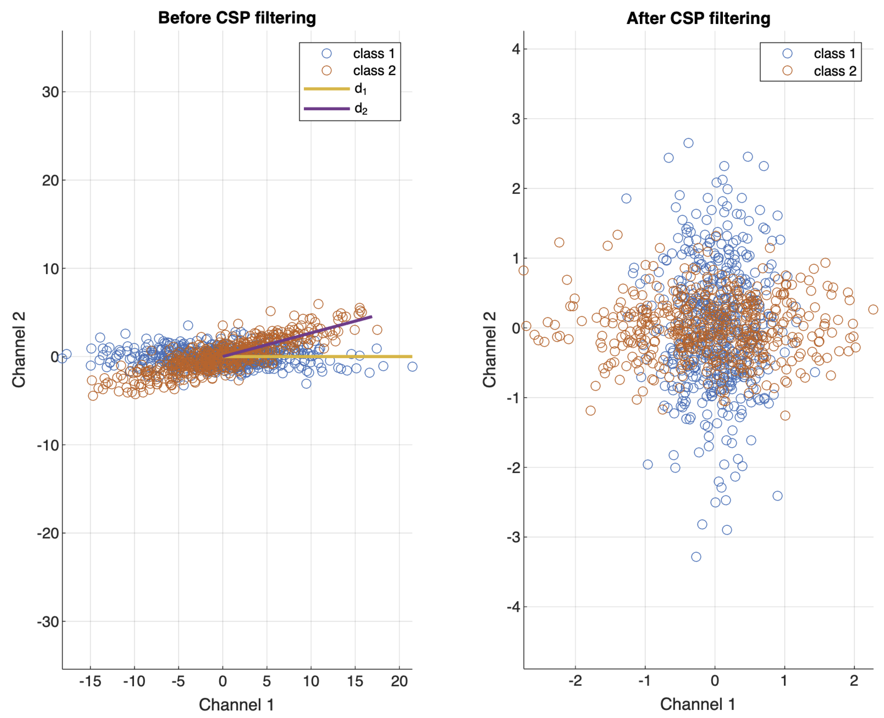
Figure 4.
Flow Chart of Genetic Algorithm
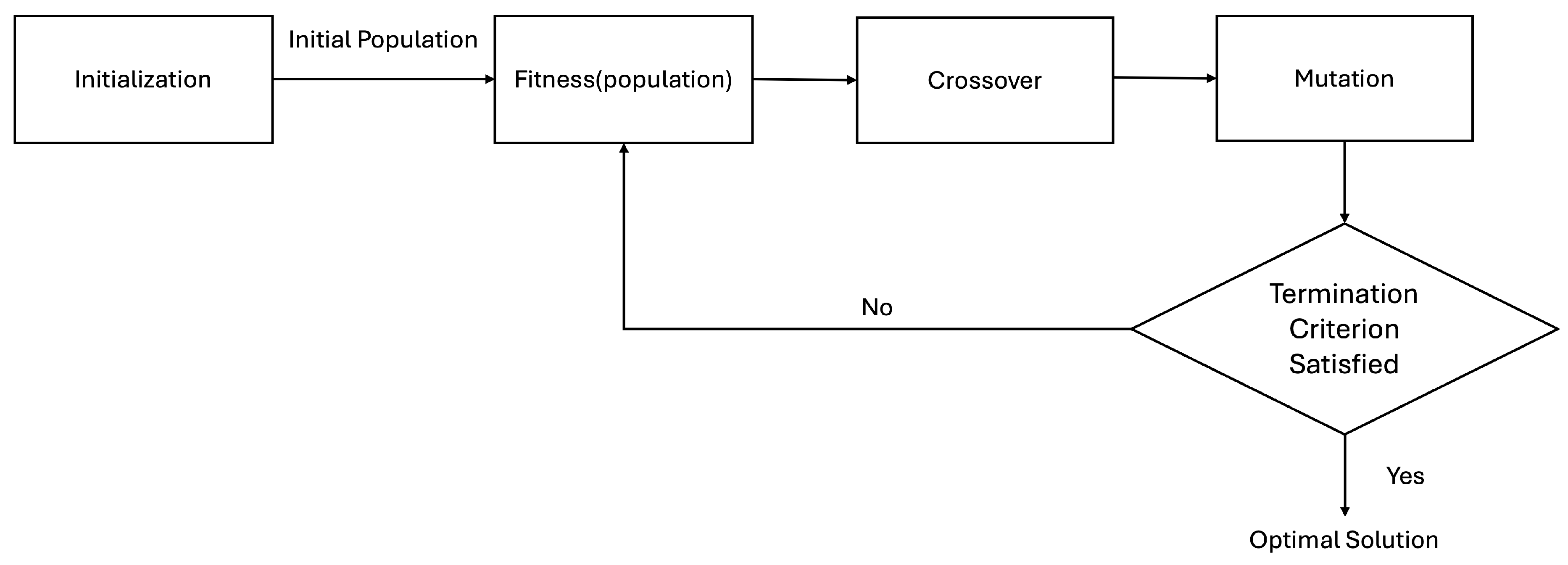
Figure 5.
Performance Comparison of SCSP Algorithms With Different r Value Across Different Channels
Figure 5.
Performance Comparison of SCSP Algorithms With Different r Value Across Different Channels
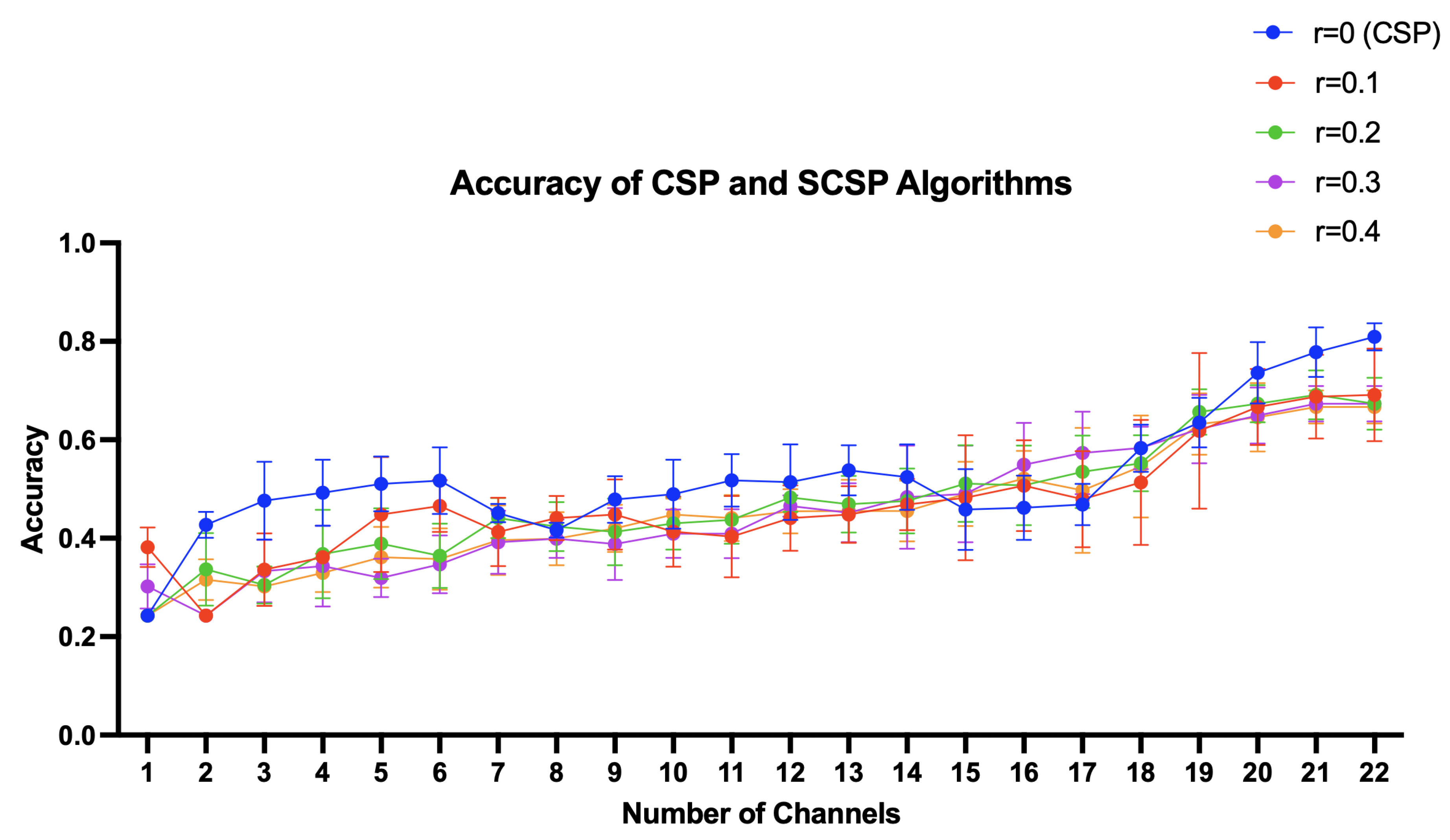
Figure 6.
Performance of CSP Based Channel Selection Methods Across Different Channels
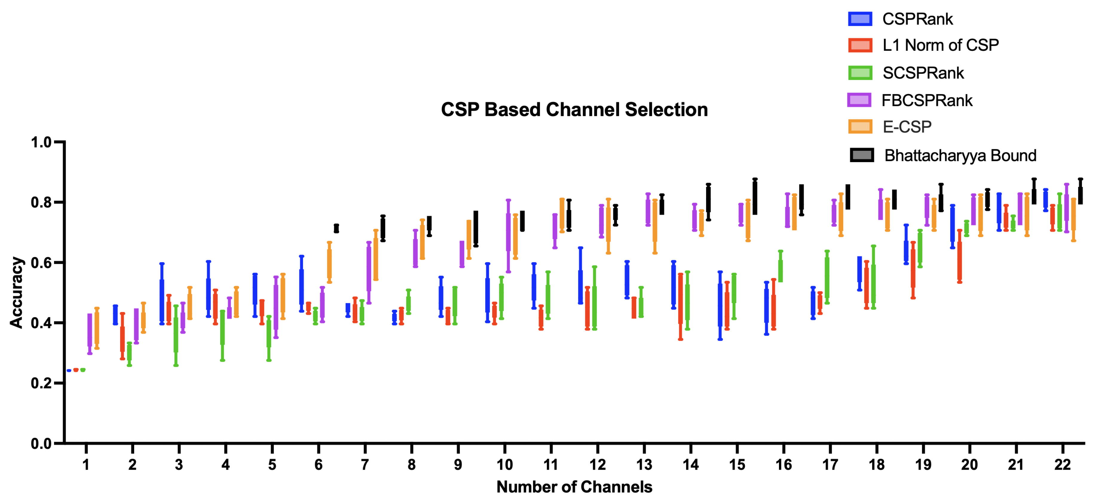
Figure 7.
Performance of Non-CSP Based Channel Selection Methods Across Different Channels
 |
Seungjun Lee is a senior student at Korea Science Academy of KAIST. His research interest is bio-signal processing, especially EEG data |
Disclaimer/Publisher’s Note: The statements, opinions and data contained in all publications are solely those of the individual author(s) and contributor(s) and not of MDPI and/or the editor(s). MDPI and/or the editor(s) disclaim responsibility for any injury to people or property resulting from any ideas, methods, instructions or products referred to in the content. |
© 2025 by the authors. Licensee MDPI, Basel, Switzerland. This article is an open access article distributed under the terms and conditions of the Creative Commons Attribution (CC BY) license (http://creativecommons.org/licenses/by/4.0/).
Copyright: This open access article is published under a Creative Commons CC BY 4.0 license, which permit the free download, distribution, and reuse, provided that the author and preprint are cited in any reuse.


