
Submitted:
21 January 2025
Posted:
21 January 2025
You are already at the latest version
Abstract
The evaluation of soil quality parameters within the Pashupathihal sub-watershed (Dharwad district) unveiled considerable spatial and chemical variability among 46 soil mapping units (SMUs) across 12 distinct soil series. The Soil Quality Index (SQI) values fluctuated between 0.20 (YSJmA1) and 0.76 (MVDmA2g2Ca). The depth of the soil varied from 35 to 180 cm (with a mean of 163.07 cm), thus indicating heterogeneity. Additionally, the CaCO₃ levels ranged from 1.37% to 14.45% (mean 6.34%), which reflected moderate calcareousness. The pH values spanned from 7.01 to 8.96 (mean 8.70), alongside high base saturation levels (between 82.35% and 92.57%, mean 90.95%), suggesting the presence of alkaline and base-rich soils. Organic carbon content, measured at 2.54 to 6.77 g/kg (mean 3.75 g/kg), was notably low, thereby affecting fertility; however, the cation exchange capacity, which ranged from 21.29 to 56.49 cmol/kg (mean 49.72 cmol/kg), demonstrated strong nutrient retention. Additionally, electrical conductivity levels ranged from 0.16 to 0.43 dS/m (mean 0.27 dS/m), confirming non-saline conditions. The exchangeable sodium percentage varied between 3.17% and 10.17% (mean 8.32%), indicating non-sodic soil types. Importantly, Bartlett’s test (χ² = 293.807, p < 0.0001) and a KMO score of 0.597 suggested that the dataset was moderately suitable for factor analysis. Principal Component Analysis (PCA) revealed three principal components that accounted for 84.82% of the variance. The radar plot emphasizes variations in soil quality parameters across SMUs; it features pronounced radial extensions that indicate superior attributes, such as depth or cation exchange capacity (for instance, MGDmA2g2Ca). The linear regression graph, reveals strong positive correlations, like the relationship between depth and CaCO₃. Nevertheless, there are also negative trends, such as organic carbon decreasing with depth. This emphasizes the intricate interplay of soil properties, which is essential for understanding soil health and functionality. Cluster analysis categorized the soil mapping units (SMUs) into four unique clusters (C1–C4) according to dissimilarities in parameters such as pH, EC and organic carbon. This process facilitated the identification of management zones. C1 indicated soils with extreme characteristics that necessitate specialized interventions; however, C3 consisted of uniform, fertile soils that are appropriate for consistent management practices. Although the distinctions among the clusters were significant, all played a role in guiding effective soil management strategies. Soil Management Units (SMUs) like MVD (127 ha, SQI 0.76) and CPT (766 ha, SQI 0.70) demonstrated elevated Soil Quality Indices (SQI); however, YSJ (5 ha, SQI 0.20) showed poor quality, primarily because of erosion and nutrient depletion. The BTP series, encompassing 2464 ha with an SQI of 0.63, covered the most extensive area, which reflects general robust soil health. Nevertheless, targeted management is essential for the low-SQI zones to improve both productivity and sustainability.
Keywords:
Soil Quality Index
; Soil Mapping Unit
; PCA
; Cluster Analysis
; Soil Depth
1. Introduction
Soil mapping units (SMUs), which are derived from LRI-based studies, play an essential role in the evaluation and prioritization of soil health indicators. Key parameters such as organic carbon (OC), cation exchange capacity (CEC) and base saturation (BS) have a significant impact on nutrient availability and retention. For instance, high CEC and BS values in particular SMUs suggest a robust ability to retain essential nutrients; this is critical for sustaining soil fertility. However, low OC levels in certain units reveal the necessity for organic matter amendments, as these amendments can enhance soil structure, microbial activity and overall productivity. Although designing soil management strategies that are tailored to the specific characteristics of SMUs may seem challenging, it ultimately ensures the effective use of resources and supports long-term agricultural sustainability, while also improving soil quality indices (Minasny and McBratney, 2016). It plays a crucial role in the precise identification of various soil challenges, including alkalinity, calcareousness and specific localized issues related to salinity or sodicity. Alkaline soils that contain high levels of calcium carbonate in certain SMUs can hinder nutrient availability particularly for vital micronutrients such as zinc and iron. Additionally, regions characterized by an elevated exchangeable sodium percentage (ESP) often experience compromised soil structure, which can lead to reduced water infiltration. Because site-specific solutions derived from SMU analysis can be employed, nutrient deficiencies may be addressed effectively, while water management strategies can be optimized, ultimately enhancing soil health significantly (Fisher, 1991).
Previous investigations into the Soil Quality Index (SQI) have largely concentrated on soil fertility parameters, highlighting crucial elements such as nutrient content, organic matter and pH to evaluate soil health. However, while these methods yield valuable insights, they frequently neglect to consider spatial variability and the intricate interplay of physical, chemical and biological properties (Granatstein and Bezdicek, 1992). Using soil mapping units (SMUs) as the foundation for SQI calculation presents a revolutionary method that addresses this shortcoming. The SMU-based SQI adopts a landscape-level viewpoint, capturing variations in texture, structure, drainage and fertility within the mapped units. This enables a more precise and geographically specific evaluation of soil quality (Drobnik et al., 2018). This approach not only aids in accurate resource management and targeted interventions but also fosters climate-resilient agricultural practices and long-term soil monitoring. The integration of SMUs with SQI creates a comprehensive framework for enhancing soil health, optimizing input usage, informing policy decisions and advancing sustainable land management (Amacher et al., 2007 and Calero et al., 2018). Although SMUs aim to provide a comprehensive framework, challenges may arise in their application. Thus, careful consideration of regional factors is essential for maximizing their impact.
Analytical tools, such as Principal Component Analysis (PCA) and regression analysis, facilitate the clustering of Soil Management Units (SMUs) based on important characteristics. This process ensures targeted interventions that effectively address regional soil variability. Radar plots, which serve as powerful visual tools, simplify the representation of multiple soil quality indicators within SMUs; they provide a clear comparison of their relative importance (Sachs, 2012). By plotting indicators like organic matter, soil depth, CEC, BS, CaCO3, EC and pH on a circular axis, radar plots enable stakeholders to easily identify strengths and weaknesses in soil quality, thus prioritizing areas for improvement. Cluster analysis, on the other hand, groups SMUs with similar soil characteristics, streamlining decision-making for region-specific soil management practices. This method helps identify patterns and variations that might otherwise be overlooked; it enables efficient resource allocation and management strategies tailored to the unique needs of different clusters (Stott et al., 2011). Similarly, linear regression graphs are invaluable for identifying relationships between soil quality indicators. However, the nuances of these relationships can sometimes be complex, which is why thorough analysis is essential. Although these tools are powerful, their effectiveness largely depends on the quality of the data used, because accurate data leads to insightful conclusions.
The addition of Soil Quality Index maps further enhances these efforts by providing a spatial visualization of SQI variations across the landscape. These maps highlight areas of high and low soil quality, enabling precise identification of regions requiring intervention or conservation. They serve as a decision-making tool for stakeholders, helping to optimize land use planning, prioritize resource allocation, and implement targeted management strategies (Scull et al., 2003). SQI maps also facilitate monitoring changes in soil quality over time, ensuring adaptive management practices that respond to evolving environmental and agricultural needs. Through the quantification of these relationships, regression analysis elucidates the most significant factors affecting soil quality. It also aids in refining Soil Quality Index (SQI) calculations for more precise and applicable outcomes. (Together, these tools integrate intricate datasets into actionable insights.) They support sustainable agricultural practices that aim to minimize chemical inputs, enhance long-term productivity and align with global food security initiatives. Leveraging radar plots, cluster analysis and regression graphs within the framework of soil mapping and precision management establishes Soil Management Units (SMUs) as a fundamental element for tackling soil variability. Furthermore, this promotes resilient, sustainable farming systems. However, the complexity of these analyses can sometimes obscure the underlying relationships, which is critical for effective implementation.
2. Material and Methods
2.1. Location of the Pashupathihal Sub-Watershed
The Dharwad district in Karnataka is located between the geographical coordinates of 15°21'54" N latitude and 75°03'39" E longitude. The area under study lies within the confines of 15°15'23" N latitude and 75°14'38" E longitude. Pashupathihal, receiving an annual rainfall of 698 mm, exhibits a gently sloping topography; its predominant soil types include sandy clay loam, clay loam and clay. This sub-watershed of Pashupathihal encompasses approximately 6129.92 hectares, situated between the latitudes of 15°06'00" N and 15°12'30" N, as well as the longitudes of 75°19'30" E and 75°25'30" E. It is bordered by the villages of Pashupathihal1, Pashupathihal2, Gudageri1, Gudageri2, Gudageri3, Gudageri4, Pashupathihal3 and Pashupathihal4 (Figure 1).
2.2. Soil Sample Collection
The initial phase encompasses the development of base maps for the Pashupathihal sub-watershed (4D5B4P), which spans approximately 6129.94 hectares and includes eight micro-watersheds. This process utilizes imagery and toposheets at scales of 1:25,000 or 1:50,000. These maps are intended to aid in delineating landforms, as they are informed by factors such as physiography, geology, land use and imagery characteristics. Field validations and soil studies conducted along transects will refine the soil legend; however, the integration of various data sources is crucial. Cadastral maps, toposheets and high-resolution WorldView imagery (0.5 m) will be procured from KSRSAC and the Survey of India, ensuring that the mapping is both precise and effective.
2.3. Soil Analysis
The evaluation of soil parameters for land resource inventory employs precise techniques for thorough soil characterization. Slope, gravel and erosion classes are categorized according to the Field Guide for Land Resource Inventory (Natarajan et al., 2016). Soil pH and electrical conductivity (EC) are established using the potentiometric method, which involves a glass electrode and conductivity bridge, in accordance with Jackson (1973). Organic carbon is assessed through the rapid titration method. Base saturation and exchangeable sodium are classified based on the USDA Keys to Soil Taxonomy (Soil Survey Staff, 2012). Cation exchange capacity and exchangeable cations are determined using the neutral normal ammonium acetate technique, whereas calcium and magnesium levels are evaluated via versenate titration and sodium and potassium are measured through flame photometry (Thomas, 1982). Free calcium carbonate (CaCO₃) is analyzed utilizing the rapid acid titration method (Piper, 2002). Diagnostic horizons, along with horizon boundaries, are recognized following the guidelines outlined in the Field Guide for Land Resource Inventory (Natarajan et al., 2016).
2.4. Field Investigation
To produce micro-watershed base maps, geo-referenced cadastral maps are superimposed onto high-resolution imagery at a scale of 1:8000. This process enables a careful delineation of landform units, which are identified based on image characteristics like tone, texture and pattern. These units undergo rigorous analysis to reveal variations in several factors: slope, erosion, soil texture, stoniness, wetness, drainage, salinity and land use practices. Field investigations are essential, as they require traversing the sub-watershed to update the base maps; however, transects and random sites are chosen for comprehensive soil profile studies. Soil profiles essentially vertical sections extending from the surface to depths of up to 200 cm are excavated at intervals intended to capture changes in slope, erosion, texture and gravel content. Although these profiles are documented using a standardized format, their morphological and physical characteristics are examined to categorize soils into series. These series represent the most homogeneous units, displaying consistent horizon development and predictable behavior under similar management conditions.
2.5. Soil Mapping Unit Selection
Each soil series is subsequently divided into phases according to characteristics such as surface soil texture, slope, erosion and stoniness. Each phase is denoted on maps through standardized symbols; however, the intricacies of these mappings are vital for effective land management. Soil samples, collected from representative pedons within each series, are subjected to laboratory characterization for thorough analysis. This process unveiling 12 soil series and delineating 46 soil mapping units in the study area is imperative for efficient watershed management and sustainable land use planning. Utilizing ArcGIS 10.8.1, comprehensive quantitative analyses were executed to produce maps delineating soil phases, mapping units and soil quality index map. This process necessitated the integration of high-resolution WorldView satellite imagery (boasting a 0.5-meter resolution at a scale of 1:8000) with Digital Elevation Model (DEM) data. The DEM offered essential terrain insights, including slope, elevation and drainage patterns; these were amalgamated with satellite-derived land cover data to enhance spatial accuracy. Descriptive analysis was carried out using MS Excel 2016 and SPSS Statistics 27 (Pallant, 2007), which facilitated the examination and summarization of soil properties, land characteristics.
2.6. Assessment of Soil Quality Index
The assessment of the Soil Quality Index (SQI) was conducted through a statistical model grounded in principal component analysis (PCA), which followed a structured process: first, defining the management objective; second, selecting pivotal indicators as a Minimum Data Set (MDS); third, assigning scores to these indicators and finally, calculating the SQI (Karlen et al., 1997).
2.7. Indicator Selection
The Principal Component Analysis (PCA) model was employed to delineate a Minimum Data Set (MDS), with the objective of simplifying the number of indicators within the model and mitigating data redundancy. This approach was selected for its inherent objectivity, as it integrates various statistical techniques, including factor analysis, cluster analysis and correlation analysis. The Soil Quality Index (SQI) of the sub-watershed underwent evaluation through soil mapping units derived from the Land Resource Inventory (LRI) study. This objective is accomplished by converting the original dataset into principal components (PCs), which are uncorrelated and systematically arranged so that the first components encapsulate the bulk of the data variation. However, PCA was chosen primarily to lessen complexity and identify the most relevant indicators for assessing the SQI, utilizing soil mapping units as a basis.
Principal components (PCs) represent a synthesis of variables that capture the greatest variation within a dataset. The methodology employed in this study aligns with prior research, which posits that PCs exhibiting high eigenvalues and variables with substantial factor loadings serve as the most accurate reflections of system characteristics. Therefore, only those PCs with eigenvalues exceeding 1 were chosen for analysis. For every PC, the associated eigenvector weight (or factor loading) was utilized to pinpoint the most critical variables for inclusion in the MDS. Variables that exhibited the highest loadings under a particular PC, along with an absolute factor loading value within 10% of the peak values, were regarded as significant. When several variables with elevated loadings were retained under a single PC, a multivariate correlation matrix was employed to compute correlation coefficients among these variables. If parameters were found to be strongly correlated (r > 0.60, p < 0.05), the variable bearing the highest loading factor was incorporated into the MDS, while others were excluded to mitigate redundancy.
2.8. Scoring of Indicators
The indicators chosen for the Minimum Data Set (MDS) were standardized to dimensionless values, ranging from 0 to 1, utilizing a linear scoring method. The ranking of these indicators depended on whether higher values were deemed favorable or unfavorable in relation to soil function. For those indicators where an increased value denoted improved performance, each data point was divided by the highest value, thereby ensuring that the maximum value received a score of 1. For indicators where lower values were preferred, each value was divided by the lowest value, resulting in the minimum receiving a score of 1. Moreover, for indicators such as pH, an "optimum" threshold value was considered. These indicators were initially scored as "higher is better" up to the threshold value (e.g., pH 7.5); however, beyond this point, they were scored as "lower is better." This scoring methodology adheres to the framework established in prior studies.
2.9. Soil Quality Index Calculation
Subsequently, the observations were transformed into numerical scores ranging from 0 to 1; these scores were then aggregated into indices for each soil sample through a weighted additive approach. To determine the suitable weight for each Principal Component (PC), the variance attributed to each PC was divided by the total variation across all PCs produced by the PCA.
The Soil Quality Index (SQI) is defined as
SQI = Σ (Principal Component Weight ∗ Individual Soil Parameter Score)
Principal Component Analysis (PCA) and descriptive statistics were executed using SPSS version 26 and Excel statistics to compute the Soil Quality (SQ) indices. This method ensures a comprehensive assessment of soil quality because it integrates multiple parameters into a cohesive framework.
3. Results and Discussion
The examination of soil parameters uncovers considerable variability in depth, CaCO₃ content, pH, organic carbon (OC), cation exchange capacity (CEC), base saturation (BS), electrical conductivity (EC) and exchangeable sodium percentage (ESP); this highlights the diverse conditions within the soil (Table 1). Depth ranges from 35 to 180 cm, with an average of 163.07 cm, indicating heterogeneity. CaCO₃ levels (ranging from 1.37 to 14.45%) reflect a moderate calcareousness, which can affect nutrient availability. The alkaline pH (7.01-8.96, mean 8.70) and elevated base saturation (82.35-92.57%, mean 90.95%) suggest soils that are predominately composed of base cations, which may lead to deficiencies in micronutrients. Although low organic carbon (2.54-6.77 g/kg, mean 3.75 g/kg) signifies poor organic matter levels, impacting soil structure and fertility, the high CEC (21.29-56.49%, mean 49.72%) indicates strong nutrient retention capacity (Qi et al., 2009). Additionally, low EC (0.16–0.43 dS/m, mean 0.27 dS/m) confirms the absence of saline conditions; however, localized salinity issues remain a concern. The ESP (3.17-10.17%, mean 8.32%) suggests non-sodic soils, but potential structural problems in areas with elevated ESP warrant further investigation. However, these practices are crucial for sustainable agricultural productivity, because they directly impact soil health (Nabiollahi et al., 2018). Although the implementation may be challenging, the benefits are undeniable.
Bartlett's test of sphericity was conducted to determine whether the correlation matrix of the dataset significantly deviates from an identity matrix (a crucial prerequisite for multivariate techniques such as factor analysis or PCA) (Table 2). The test produced an observed chi-square value of 293.807, which far exceeds the critical value of 41.337 at 28 degrees of freedom; this finding, along with a highly significant p-value (<0.0001), leads to the rejection of the null hypothesis. Thus, it indicates that the variables are significantly intercorrelated, implying that the correlation matrix is not an identity matrix (Dai et al., 2018). This result affirms the dataset suitability for dimensionality reduction techniques, because it suggests the existence of latent structures or factors that explain the variance. However, while Bartlett's test confirms significant correlations, it should be supplemented with the Kaiser-Meyer-Olkin (KMO) measure to achieve a more comprehensive assessment of sampling adequacy before moving forward with factor analysis.
The Kaiser-Meyer-Olkin (KMO) measure of sampling adequacy was computed to evaluate the dataset's suitability for factor analysis (Table 3). The overall KMO value of 0.597 signifies a mediocre level of adequacy. Variable-specific KMO values fluctuated from 0.354 (for ESP) to 0.874 (for OC). Notably, the higher values observed for OC (0.874) and BS (0.807) imply that these variables are particularly well-suited for factor analysis. However, the lower values for EC (0.377) and ESP (0.354) suggest a significant lack of sampling adequacy for these variables. Variables like Depth (0.652), pH (0.537) and CEC (0.593) demonstrate moderate adequacy. The overall KMO score, although it approaches the threshold of acceptability (0.6), indicates that while factor analysis could be undertaken, the dataset might benefit from refinement (Khan et al., 2022). This could involve excluding variables with low KMO scores (for instance, EC and ESP) or gathering additional data to bolster sampling adequacy. These findings, when considered alongside Bartlett’s test of sphericity, suggest that while factor analysis is a viable option, enhancements to the dataset would contribute to its reliability and robustness.
The principal component analysis (PCA) conducted on soil quality parameters revealed eight distinct components (Table 4). The initial three components (PC1, PC2 and PC3) accounted for 51.92%, 19.44% and 13.47% of the overall variability, respectively; this results in a cumulative explanation of 84.82% of the total variance. However, the remaining components contributed only marginally. PC1, characterized by a strong positive loading for Depth (0.885), pH (0.887), CEC (0.871) and BS (0.872), represents the overall soil fertility and structural stability. PC2, driven by significant loadings for CaCO₃ (0.816) and moderate contributions from BS (0.268), underscores the calcareous nature of the soil and its effects on nutrient availability. In contrast, PC3 is defined by a high positive loading for EC (0.813) and negative loadings for ESP (-0.536), which indicates complex relationships between salinity and sodicity. The negative loading of OC (-0.796) in PC1 suggests a tension between organic matter and fertility parameters, likely attributable to external management practices or natural decomposition processes. Furthermore, the eigenvalue exceeding 1 for the first three principal components confirms their significance (Erkossa et al., 2007 and Vasu et al., 2016). Although the contributions from PC4 and subsequent components are low, this indicates a diminishing explanatory power. These outcomes illustrate the intricate relationship between physical and chemical soil characteristics; PC1 serves as the primary determinant of soil quality. However, PC2 and PC3 highlight particular issues, such as calcareousness (which can exacerbate problems) and salinity. This dual emphasis informs targeted soil management strategies, although the complexities involved require careful consideration (De Laurentiis et al., 2019 and Sheidai Karkaj et al., 2019). Because of these factors, understanding soil properties becomes essential for effective agricultural practices.
The scree plot (which illustrates the variation of eigenvalues in relation to principal components) reveals a pronounced decline in eigenvalues from PC1 to PC3; however, this is followed by a gradual leveling off (Figure 2). This pattern indicates the importance of the initial three components in elucidating the dataset's variance. Specifically, PC1 possesses the highest eigenvalue (4.154), accounting for 51.92% of the variability. In contrast, PC2 shows an eigenvalue of 1.555 (19.44%) and PC3 has an eigenvalue of 1.077 (13.47%), together cumulatively representing 84.82% of the overall variance. Beyond PC3, the eigenvalues descend below 1, revealing minimal contributions from PC4 to PC8, which suggests that these components provide negligible explanatory power. Although the elbow point on the scree plot is situated at PC3, it confirms that the first three components effectively capture the majority of the variability, thus proving adequate for summarizing soil quality. This pattern highlights the significance of concentrating on PC1 (which is dominated by parameters such as depth, pH, CEC and BS) for assessing overall soil fertility. In contrast, PC2 (which is influenced by CaCO₃ and BS) pertains to calcareousness and nutrient availability, while PC3 (which is linked to EC and ESP) relates to salinity and sodicity. The sharp decline in eigenvalues indicates a decreasing influence of additional components (Raiesi and Kabiri, 2016). This reinforces the rationale for reducing dimensionality to three principal components when evaluating soil quality and constructing indices. However, this approach facilitates effective and economical representation of the dataset.
The correlation matrix offers valuable insights into the relationships among various soil quality parameters; significant correlations are emphasized at a significance level of alpha = 0.05. Depth demonstrates a robust positive correlation with pH (0.7), CEC (0.748) and BS (0.657), which indicates that deeper soils tend to be more fertile and alkaline (Table 5 and Figure 3). This is likely because of enhanced nutrient retention and base saturation. CaCO₃ presents moderate positive correlations with pH (0.488) and BS (0.378), reflecting the role of calcium carbonate in influencing soil alkalinity and base cation levels. Moreover, pH exhibits a strong correlation with BS (0.832) and CEC (0.748), underscoring how alkalinity can affect nutrient exchange capacity and base saturation. However, organic carbon (OC) reveals significant negative correlations with pH (-0.65), CEC (-0.539) and BS (-0.736), suggesting that increased organic matter is associated with lower alkalinity and diminished base saturation (Karlen et al., 2001). This could be due to acidic organic residues or certain management practices, although the precise mechanisms may vary. EC displays weak and statistically nonsignificant correlations with most parameters, with the exception of a modest positive correlation with Depth (0.444). This suggests that salinity is not significantly affected by other soil properties in the current dataset. In contrast, ESP shows a moderate correlation with both Depth (0.603) and CEC (0.639), implying that sodicity tends to rise as soil depth increases and nutrient retention capacity is enhanced. However, its weak correlation with BS (0.288) highlights potential variability in sodium saturation. These interrelations indicate a complex interplay among soil chemical and physical properties, where depth and pH are predominant factors influencing soil fertility; moreover, organic carbon appears to inversely affect nutrient cycling (Simon et al., 2022). Because of these findings, it is essential to manage organic matter and salinity effectively to enhance soil quality, while also taking advantage of the naturally elevated CEC and BS for optimal crop production.
The cluster plot of all soil mapping units (SMUs) delineates the soils into four distinct clusters: C1, C2, C3 and C4, based on their dissimilarity (Figure 4). This dissimilarity likely stems from parameters such as pH, EC, organic carbon, texture and nutrient levels. Cluster C1, which represents SMUs with the highest dissimilarity, indicates unique or extreme soil properties (for example, high salinity, sodicity, or poor fertility), thus requiring specialized management techniques. Clusters C2 and C4 exhibit moderate dissimilarity; these clusters suggest soils with varying, but moderately similar, characteristics such as nutrient availability, drainage, or texture that necessitate tailored practices. Cluster C3, characterized by minimal dissimilarity, indicates highly homogeneous and likely fertile soils, suitable for uniform management practices. These groupings not only facilitate the identification of potential soil management zones but also guide precise interventions necessary for sustainable agriculture (Vasu et al., 2024). The results underscore the necessity for targeted strategies for distinct soils (like C1) while optimizing inputs for the more uniform clusters (C2, C3 and C4), thereby supporting efficient resource use and enhancing productivity; however, it is crucial to recognize the unique demands of each cluster (Askari and Holden, 2015).
The scatter plot exemplifies the intricate relationships between soil depth and various soil quality parameters (such as CaCO₃, pH, OC, CEC, BS, EC, ESP) derived from the training set (Figure 5). Each parameter is depicted through differently colored data points, with corresponding fitted lines illustrating the model's predictions. Notably, the model reveals a robust positive correlation between CaCO₃ and depth; this suggests that deeper soils tend to possess higher calcium carbonate content. In contrast, CEC demonstrates a moderate positive relationship with depth, indicating an increased cation exchange capacity in deeper soils. pH shows a slight positive correlation, possibly because of heightened alkalinity in deeper layers. On the other hand, organic carbon (OC) exhibits a slight negative correlation, which is consistent with the presence of more organic matter in surface soils (McBratney et al., 2003). Furthermore, base saturation (BS) indicates a slight positive correlation, implying improved base saturation in deeper soils. However, electrical conductivity (EC) and exchangeable sodium percentage (ESP) reveal weak or negligible correlations with depth, suggesting a limited influence of depth on these specific parameters (Letey et al., 2003). Overall, the narrative underscores significant relationships regarding soil depth—(for instance), the robust correlation between CaCO₃ and depth, as well as the inverse relationship between OC and depth. This suggests potential areas for further exploration in soil management. However, it is essential to consider these factors carefully, because they may influence agricultural practices. Although the findings are compelling, further research is necessary to fully understand these dynamics.
The radar plot serves as a visual tool to illustrate the variation in soil quality parameters across diverse soil mapping units (SMUs). Notably, SMUs exhibiting more pronounced radial extensions (i.e., longer lines) in specific directions correspond to elevated values for those parameters (Figure 6). For example, SMUs such as "VSmA1" and "YSJmA1" demonstrate significant extensions along the Depth axis, which indicates the presence of deeper soils; however, other units, like "MGDmA2g2Ca," display extended lines along parameters such as CEC, thereby reflecting a higher cation exchange capacity. This suggests that these SMUs possess enhanced soil fertility. On the other hand, SMUs like "CPTmA1" exhibit shorter radial extensions in parameters including OC, EC and ESP, which implies lower organic carbon content, reduced salinity and less sodicity. Although this could indicate less fertile or more challenging soils, the overall implications warrant further investigation. The radar plot facilitates a rapid comparison of the performance of each SMU (Soil Management Unit) across diverse soil properties (Metwaly et al., 2024). This assists in discerning which units might necessitate amendments or management interventions. SMUs that extend further along the "BS" (Base Saturation) and "pH" axes tend to demonstrate favorable conditions for nutrient availability and soil structure. However, those with shorter extensions in parameters like EC (Electrical Conductivity) and ESP (Exchangeable Sodium Percentage) may indicate challenges related to salinity and sodicity, which could, in turn, hinder crop growth (Barikloo et al., 2024). Although the radar plot serves as a valuable tool for visualizing and comparing overall soil health and quality, it also facilitates the development of targeted soil management strategies.
The Soil Quality Index (SQI) values across diverse soil mapping units (SMUs) demonstrate significant variability in soil quality; in fact, these values span from 0.20 (YSJmA1) to 0.76 (MVDmA2g2Ca). A considerable number of SMUs cluster around the SQI value of 0.70, which suggests that they possess relatively good soil quality (Table 6). This includes units such as CPTmA2g2Ca, CPTmB2 and MGDmA1, among others. However, units that exceed an SQI value of 0.70, like MVDmA2g2Ca (0.76), signify superior soil quality likely because of advantageous physical and chemical characteristics, such as optimal pH, organic carbon content and cation exchange capacity. Conversely, units with lower SQI values, including YSJmA1 (0.20), reflect inferior soil conditions, possibly influenced by factors like reduced organic matter, elevated salinity, or inadequate nutrient availability (Andrews and Carroll, 2001). The predominance of SQI values around 0.70 indicates that most soil mapping units exhibit moderately good soil quality; but, targeted soil management practices could improve the quality of those with lower SQI values. Although the variation in SQI across different units is notable, it highlights the necessity for site-specific management strategies to enhance soil fertility and sustainability (Valani et al., 2020). The scoring indicators for soil mapping units are categorized as follows: higher is better are preferred for pH, depth, base saturation (BS), and cation exchange capacity (CEC), whereas lower is better are desirable for calcium carbonate (CaCO3) and electrical conductivity (EC).
The Soil Quality Index (SQI) map of the Pashupathihal Sub-watershed, situated in Dharwad district, demonstrates considerable spatial variability in soil quality across twelve distinct soil series (46 soil mapping unit). These series are classified into high, medium and low SQI categories, primarily due to specific soil characteristics (Figure 7). Notably, the BTP series covering the largest area of 2464 ha (40.20%) displays an SQI of 0.63, thereby categorizing it as high-quality. This indicates a strong level of soil health and suitability for agricultural endeavors. Other series, including CPT (766 ha, 12.49%, SQI 0.70), HMB (84 ha, 1.37%, SQI 0.72), KNL (106 ha, 1.73%, SQI 0.69), KPR (369 ha, 6.02%, SQI 0.65), LDk (1524 ha, 24.85%, SQI 0.70), MVD (127 ha, 2.07%, SQI 0.76) and NGT (352 ha, 5.75%, SQI 0.72), also fall within this high-quality classification. These series reflect favorable conditions such as enhanced organic matter content, efficient drainage and effective management practices however, it is essential to note that variations exist among them (Zhao et al., 2021; Olaniyan and Ogunkunle, 2007). Although the overall trends are positive, localized factors may influence individual series differently. However, VRV (26 ha, 0.42%, SQI 0.37) and GDA (1 ha, 0.01%, SQI 0.42) are categorized within the medium-quality class, likely attributable to moderate erosion levels or nutrient availability. Although the YSJ series encompasses only 5 ha (0.08%) and exhibits a remarkably low SQI of 0.20, it is classified as low-quality. This classification highlights underlying problems, such as poor drainage, substantial erosion, or nutrient depletion (Mandal et al., 2011 and Kalambukattu et al., 2018). The majority of the sub-watershed reveals elevated SQI values (indicating the implementation of sustainable management practices); however, the low-SQI zones particularly the YSJ series require immediate action. This is essential because interventions, including soil conservation techniques and fertility restoration, are critical for enhancing productivity, although several challenges persist.
4. Conclusions
The examination of soil parameters reveals considerable variability in depth, pH, CaCO₃ content, OC, CEC, BS, EC and ESP across various SMUs. Deeper soils generally exhibit enhanced fertility and alkalinity, attributable to elevated CEC and BS; they often present low OC levels. This highlights the critical need for effective management of surface-level organic matter. Moderate CaCO₃ levels imply calcareousness, while alkaline pH and increased BS may point to potential micronutrient deficiencies. Low EC and ESP typically indicate non-saline, non-sodic soils, although localized salinity and structural problems in certain areas necessitate ongoing monitoring. The principal component analysis (PCA) uncovers three central components PC1 (soil fertility and structural stability), PC2 (calcareousness) and PC3 (salinity and sodicity) which collectively account for 84.82% of the variance. This enables more targeted interventions for sustainable soil management.
The categorization of SMUs into distinct clusters offers valuable insights for the implementation of targeted soil management practices. Clusters exhibiting high dissimilarity, such as C1, necessitate intensive management due to issues related to salinity, sodicity, or fertility. More homogeneous clusters like C3 tend to benefit from uniform management practices. The Soil Quality Index (SQI) values, which range from 0.20 to 0.76, further highlight the variability in soil health; remarkably, moderately good soils are often found clustering around a value of 0.70. Strategies designed to enhance lower-SQI units may include balanced fertilization, the enrichment of organic matter and the mitigation of salinity or alkalinity problems. Visual tools, such as radar and scatter plots, are instrumental in pinpointing the strengths and weaknesses of specific SMUs, thereby facilitating precise and efficient resource allocation. Implementing these targeted strategies, specific to each cluster, will not only improve soil fertility but also enhance sustainability supporting optimal crop production and long-term agricultural productivity.
The Pashupathihal Sub-watershed predominantly demonstrates a high level of soil quality; the BTP series occupies the most extensive area and indicates advantageous conditions for agricultural activities. However, localized challenges exist in zones with low soil quality index (SQI), especially the YSJ series, which highlights the necessity for specific soil conservation and fertility enhancement strategies. Sustainable management practices must be bolstered to preserve and enhance soil health throughout this watershed, because the long-term viability of agriculture relies on such efforts.
References
- Amacher, M.C.; ONeil, K.P.; Perry, C.H. 2007. Soil vital signs: a new soil quality index (SQI) for assessing forest soil health. Res. Pap. RMRS-RP-65. Fort Collins, CO: US Department of Agriculture, Forest Service, Rocky Mountain Research Station. 12 p., 65.
- Andrews, S.S.; Carroll, C.R. Designing a soil quality assessment tool for sustainable agroecosystem management. Ecological Applications 2001, 11, 1573–1585. [Google Scholar] [CrossRef]
- Askari, M.S.; Holden, N.M. Quantitative soil quality indexing of temperate arable management systems. Soil and Tillage Research 2015, 150, 57–67. [Google Scholar] [CrossRef]
- Barikloo, A.; Alamdari, P.; Rezapour, S.; Taghizadeh-Mehrjardi, R. Digital mapping of soil quality index to evaluate orchard fields using random forest models. Modeling Earth Systems and Environment 2024, 1–17. [Google Scholar] [CrossRef]
- Calero, J.; Aranda, V.; Montejo-Raez, A.; Martin-Garcia, J.M. A new soil quality index based on morpho-pedological indicators as a site-specific web service applied to olive groves in the Province of Jaen (South Spain). Computers and Electronics in Agriculture 2018, 146, 66–76. [Google Scholar] [CrossRef]
- Dai, F.; Lv, Z.; Liu, G. Assessing soil quality for sustainable cropland management based on factor analysis and fuzzy sets: A case study in the Lhasa River Valley, Tibetan Plateau. Sustainability 2018, 10, 3477. [Google Scholar] [CrossRef]
- De Laurentiis, V.; Secchi, M.; Bos, U.; Horn, R.; Laurent, A.; Sala, S. Soil quality index: Exploring options for a comprehensive assessment of land use impacts in LCA. Journal of Cleaner Production 2019, 215, 63–74. [Google Scholar] [CrossRef]
- Drobnik, T.; Greiner, L.; Keller, A.; Gret-Regamey, A. Soil quality indicators–From soil functions to ecosystem services. Ecological indicators 2018, 94, 151–169. [Google Scholar] [CrossRef]
- Erkossa, T.; Itanna, F.; Stahr, K. Indexing soil quality: a new paradigm in soil science research. Soil Research 2007, 45, 129–137. [Google Scholar] [CrossRef]
- Fisher, P.F. Modelling soil map-unit inclusions by Monte Carlo simulation. International Journal of Geographical Information System 1991, 5, 193–208. [Google Scholar] [CrossRef]
- Granatstein, D.; Bezdicek, D.F. The need for a soil quality index: local and regional perspectives. American Journal of Alternative Agriculture 1992, 7, 12–16. [Google Scholar] [CrossRef]
- Jackson, M.L. 1973. Soil Chemical Analysis. Prentice hall of India private limited, New Delhi, 498.
- Kalambukattu, J.G.; Kumar, S.; Ghotekar, Y.S. Spatial variability analysis of soil quality parameters in a watershed of Sub-Himalayan Landscape-A case study. Eurasian Journal of Soil Science 2018, 7, 238–250. [Google Scholar] [CrossRef]
- Karlen, D.L.; Andrews, S.S.; Doran, J.W. 2001. Soil quality: Current concepts and applications.
- Karlen, D.L.; Mausbach, M.J.; Doran, J.W.; Cline, R.G.; Harris, R.F.; Schuman, G.E. Soil quality: a concept, definition, and framework for evaluation (a guest editorial). Soil Science Society of America Journal 1997, 61, 4–10. [Google Scholar] [CrossRef]
- Khan, J.; Singh, R.; Upreti, P.; Yadav, R.K. Geo-statistical assessment of soil quality and identification of Heavy metal contamination using Integrated GIS and Multivariate statistical analysis in Industrial region of Western India. Environmental Technology & Innovation 2022, 28, 102646. [Google Scholar]
- Letey, J.; Sojka, R.E.; Upchurch, D.R.; Cassel, D.K.; Olson, K.R.; Payne, W.A.; Petrie, S.E.; Price, G.H.; Reginato, R.J.; Scott, H.D.; Smethurst, P.J. Deficiencies in the soil quality concept and its application. Journal of soil and water conservation 2003, 58, 180–187. [Google Scholar]
- Mandal, U.K.; Ramachandran, K.; Sharma, K.L.; Satyam, B.; Venkanna, K.; Udaya Bhanu, M.; Mandal, M.; Masane, R.N.; Narsimlu, B.; Rao, K.V.; Srinivasarao, C. Assessing soil quality in a semiarid tropical watershed using a geographic information system. Soil Science Society of America Journal 2011, 75, 1144–1160. [Google Scholar] [CrossRef]
- McBratney, A.B.; Santos, M.M.; Minasny, B. On digital soil mapping. Geoderma 2003, 117, 3–52. [Google Scholar] [CrossRef]
- Metwaly, M.M.; Metwalli, M.R.; Abd-Elwahed, M.S.; Zakarya, Y.M. Digital mapping of soil quality and salt-affected soil indicators for sustainable agriculture in the Nile Delta region. Remote Sensing Applications: Society and Environment 2024, 36, 101318. [Google Scholar] [CrossRef]
- Minasny, B.; McBratney, A.B. Digital soil mapping: A brief history and some lessons. Geoderma 2016, 264, 301–311. [Google Scholar] [CrossRef]
- Nabiollahi, K.; Taghizadeh-Mehrjardi, R.; Eskandari, S. Assessing and monitoring the soil quality of forested and agricultural areas using soil-quality indices and digital soil-mapping in a semi-arid environment. Archives of Agronomy and soil science 2018, 64, 696–707. [Google Scholar] [CrossRef]
- Natarajan, A.; Reddy, R.S.; Niranjana Hedge, R.; Shrinivasan, R.; Dharumarajan, S.; Srinivas, S.; Dhanorkar, B.A. Vasundhara., 2016. Field Guide for Land Resource Inventory, SUJALA III Project, Karnataka NBSS Publ. No. ICAR-NBSS and LUP, Bangalore, 154.
- Olaniyan, J.O.; Ogunkunle, A.O. An evaluation of the soil map of Nigeria:, I.I. Purity of mapping unit. Journal of World Association of Soil and Water Conservation J 2007, 2, 97–108. [Google Scholar]
- Pallant, J. 2007, SPSS Survival Manual: A Step by Step Guide to Data Analysis Using SPSS for Windows Version 15; Open University Press: Berkshire, UK, p. 165.
- Piper, C.S. 2002. Soil and Plant Analysis, Hans Publishers, Bombay, 368.
- Qi, Y.; Darilek, J.L.; Huang, B.; Zhao, Y.; Sun, W.; Gu, Z. Evaluating soil quality indices in an agricultural region of Jiangsu Province, China. Geoderma 2009, 149, 325–334. [Google Scholar] [CrossRef]
- Raiesi, F.; Kabiri, V. Identification of soil quality indicators for assessing the effect of different tillage practices through a soil quality index in a semi-arid environment. Ecological Indicators 2016, 71, 198–207. [Google Scholar] [CrossRef]
- Sachs, L. 2012. Applied statistics: a handbook of techniques. Springer Science & Business Media.
- Scull, P.; Franklin, J.; Chadwick, O.A.; McArthur, D. Predictive soil mapping: a review. Progress in Physical geography 2003, 27, 171–197. [Google Scholar] [CrossRef]
- Sheidai Karkaj, E.; Sepehry, A.; Barani, H.; Motamedi, J.; Shahbazi, F. Establishing a suitable soil quality index for semi-arid rangeland ecosystems in northwest of Iran. Journal of Soil Science and Plant Nutrition 2019, 19, 648–658. [Google Scholar] [CrossRef]
- Simon, C.D.P.; Gomes, T.F.; Pessoa, T.N.; Soltangheisi, A.; Bieluczyk, W.; Camargo, P.B.D.; Martinelli, L.A.; Cherubin, M.R. Soil quality literature in Brazil: A systematic review. Revista Brasileira de Ciencia do Solo 2022, 46, e0210103. [Google Scholar] [CrossRef]
- Soil Survey Staff. 2012. Keys to Soil Taxonomy, United States Department of Agriculture Natural Resource Conservation Service, 12th Edition, Washington D.C., USA.
- Stott, D.E.; Cambardella, C.A.; Tomer, M.D.; Karlen, D.L.; Wolf, R. A soil quality assessment within the Iowa River South Fork watershed. Soil Science Society of America Journal 2011, 75, 2271–2282. [Google Scholar] [CrossRef]
- Thomas, G.W.; 1982 Exchangeable Cations In: Methods of soil survey part, I.I. Chemical and Microbiological properties. American Society of Agronomy, Madison, Wisconsin, USA, 159-164.
- Valani, G.P.; Vezzani, F.M.; Cavalieri-Polizeli, K.M.V. Soil quality: Evaluation of on-farm assessments in relation to analytical index. Soil and Tillage Research 2020, 198, 104565. [Google Scholar] [CrossRef]
- Vasu, D.; Singh, S.K.; Ray, S.K.; Duraisami, V.P.; Tiwary, P.; Chandran, P.; Nimkar, A.M.; Anantwar, S.G. Soil quality index (SQI) as a tool to evaluate crop productivity in semi-arid Deccan plateau, India. Geoderma 2016, 282, 70–79. [Google Scholar] [CrossRef]
- Vasu, D.; Tiwary, P.; Chandran, P. A novel and comprehensive soil quality index integrating soil morphological, physical, chemical, and biological properties. Soil and Tillage Research 2024, 244, 106246. [Google Scholar] [CrossRef]
- Zhao, X.; Tong, M.; He, Y.; Han, X.; Wang, L. A comprehensive, locally adapted soil quality indexing under different land uses in a typical watershed of the eastern Qinghai-Tibet Plateau. Ecological Indicators 2021, 125, 107445. [Google Scholar] [CrossRef]
Figure 1.
Location map of the Pashupathihal Sub-watershed.
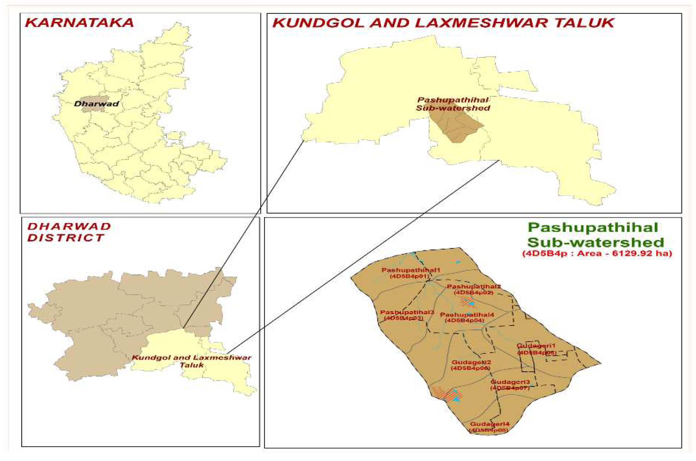
Figure 2.
representative scree plot showing variation of eigenvalues with soil component for soil quality index.
Figure 2.
representative scree plot showing variation of eigenvalues with soil component for soil quality index.
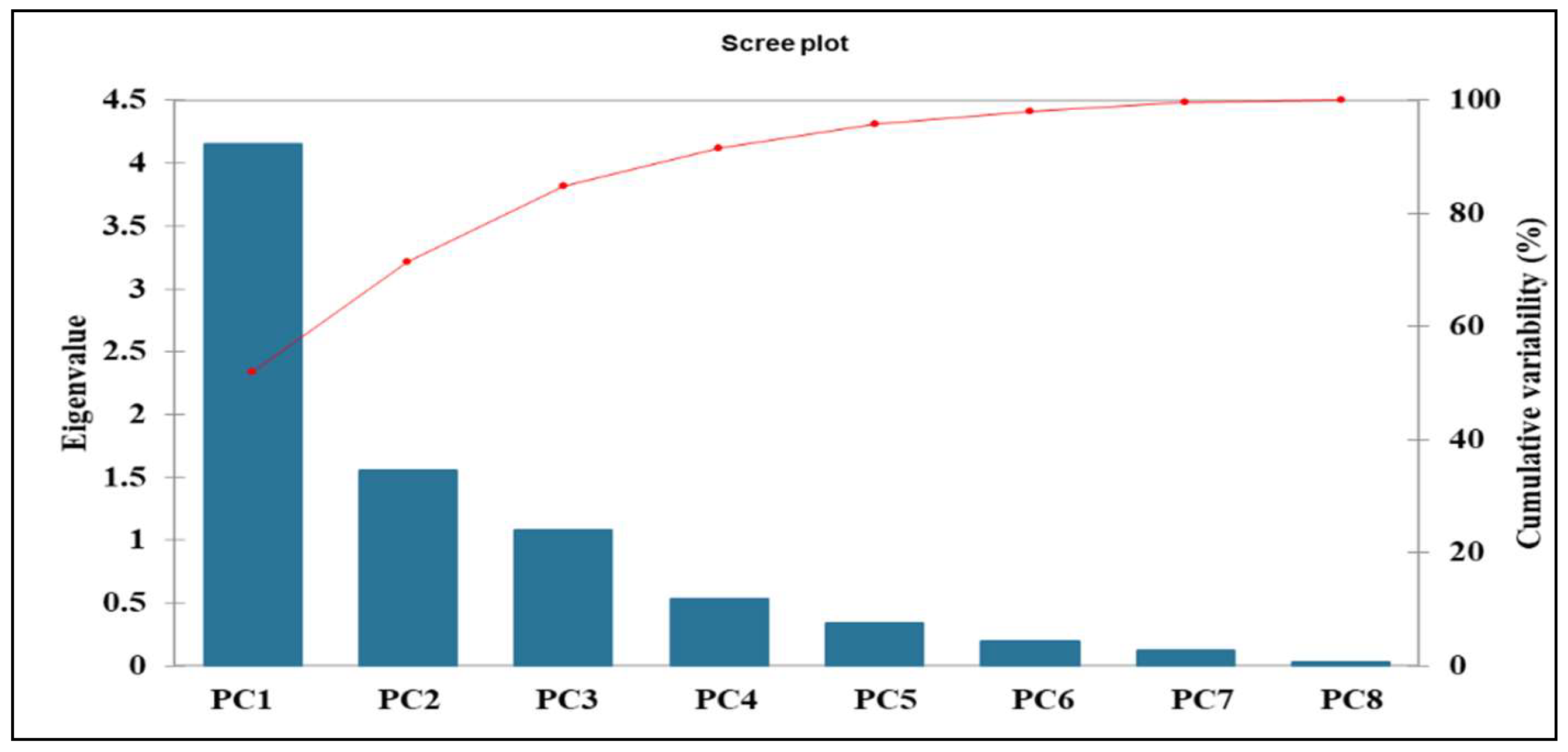
Figure 3.
Correlation between soil quality paramteres.
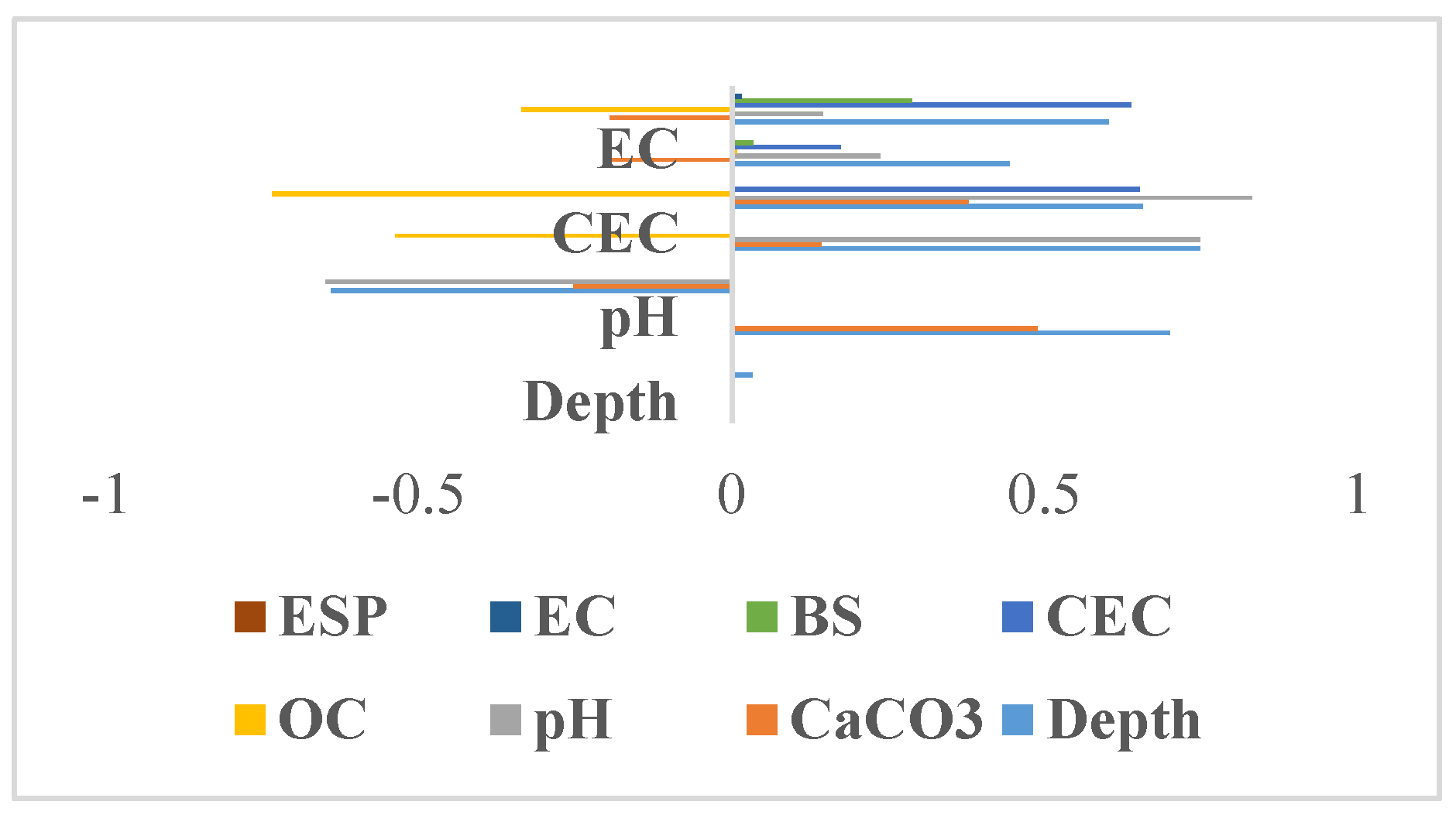
Figure 4.
Cluster plot of soil mapping units selected for soil quality index.
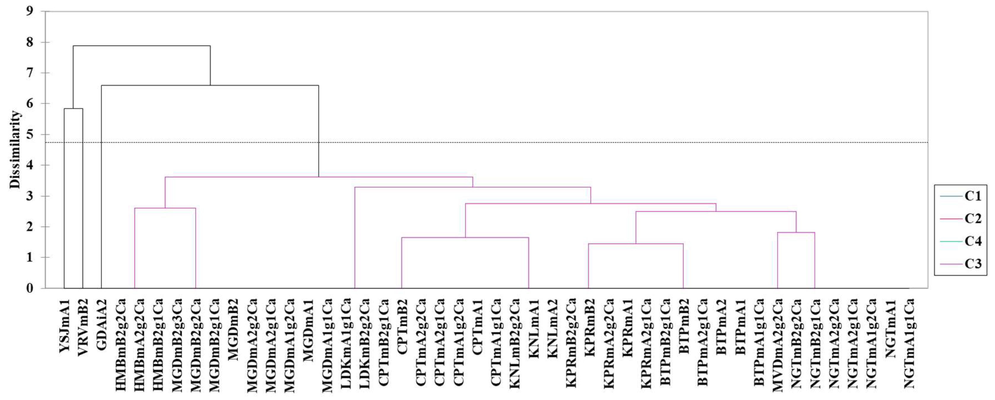
Figure 5.
Linear regression graph represents the relationship between soil mapping units parameters.
Figure 5.
Linear regression graph represents the relationship between soil mapping units parameters.
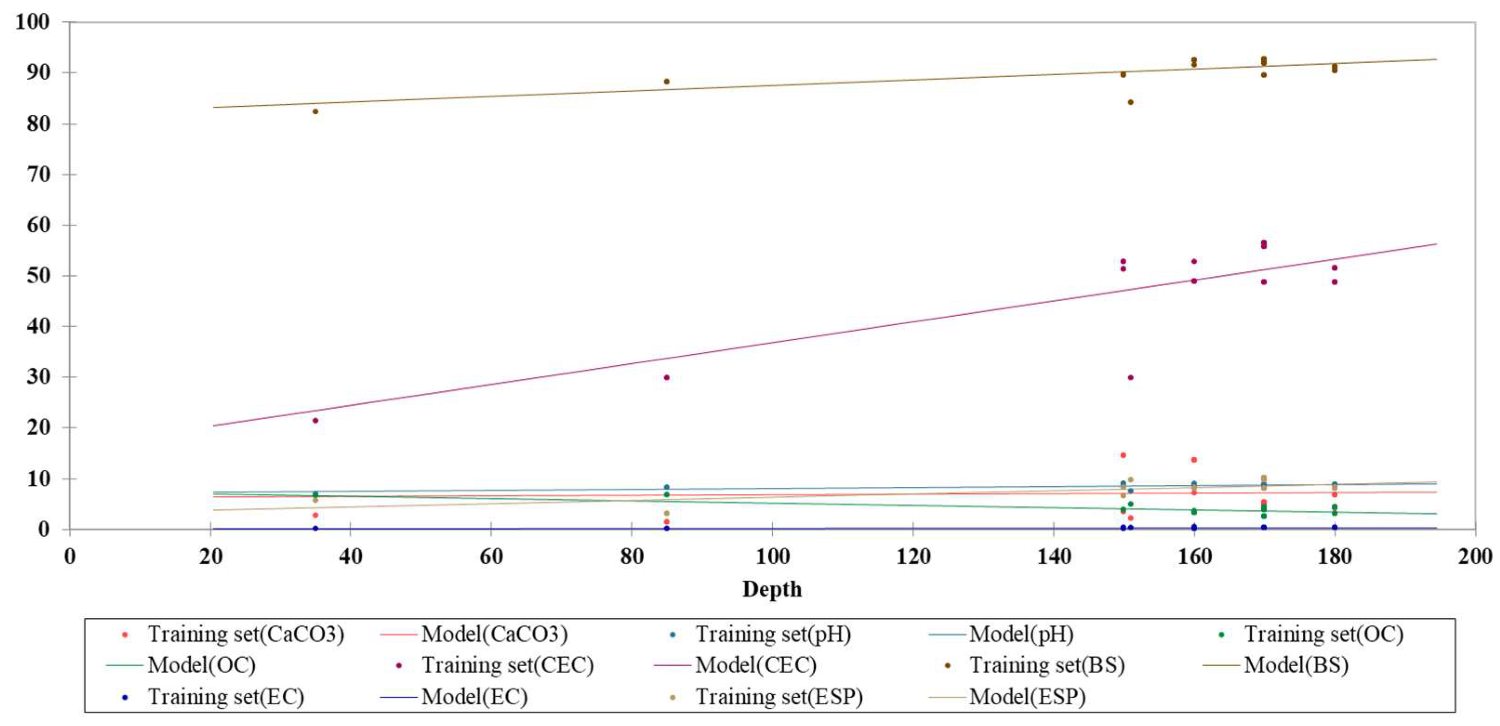
Figure 6.
Radar plot of soil mapping units selected for soil quality index.
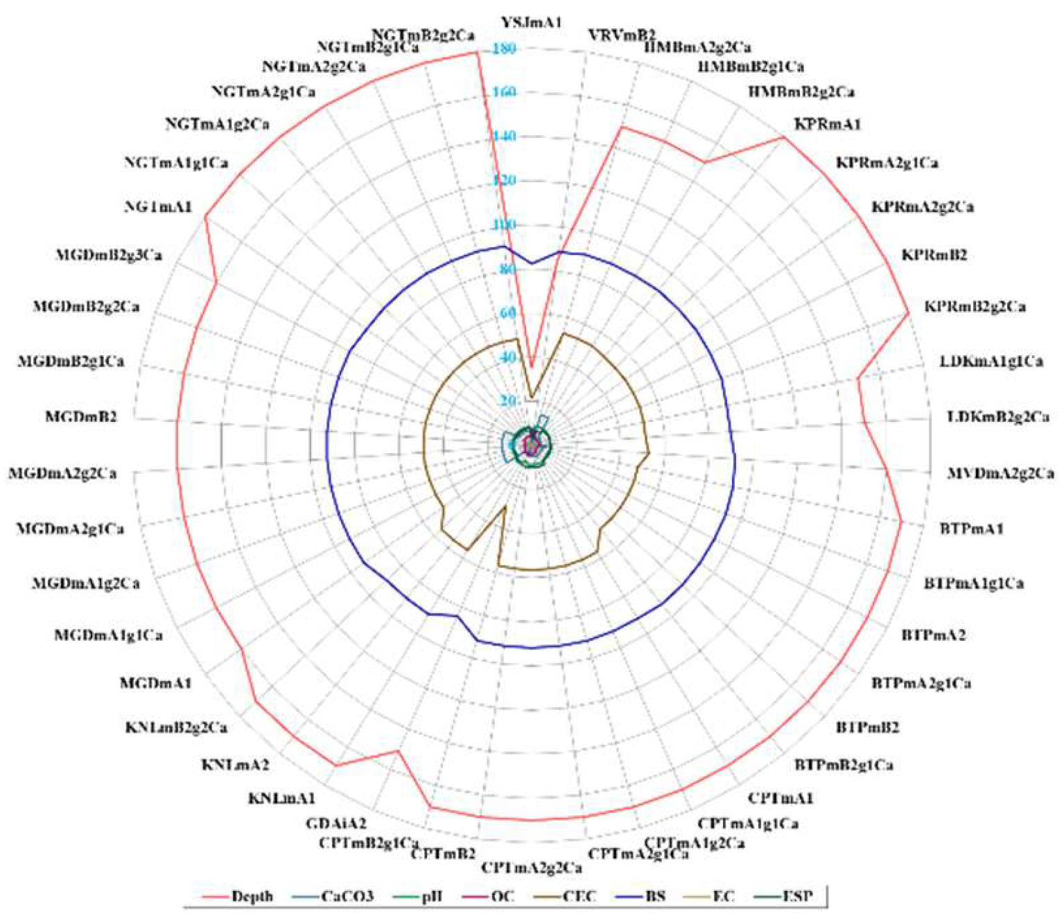
Figure 7.
Soil quality index map of Pashupathihal Sub-watershed.
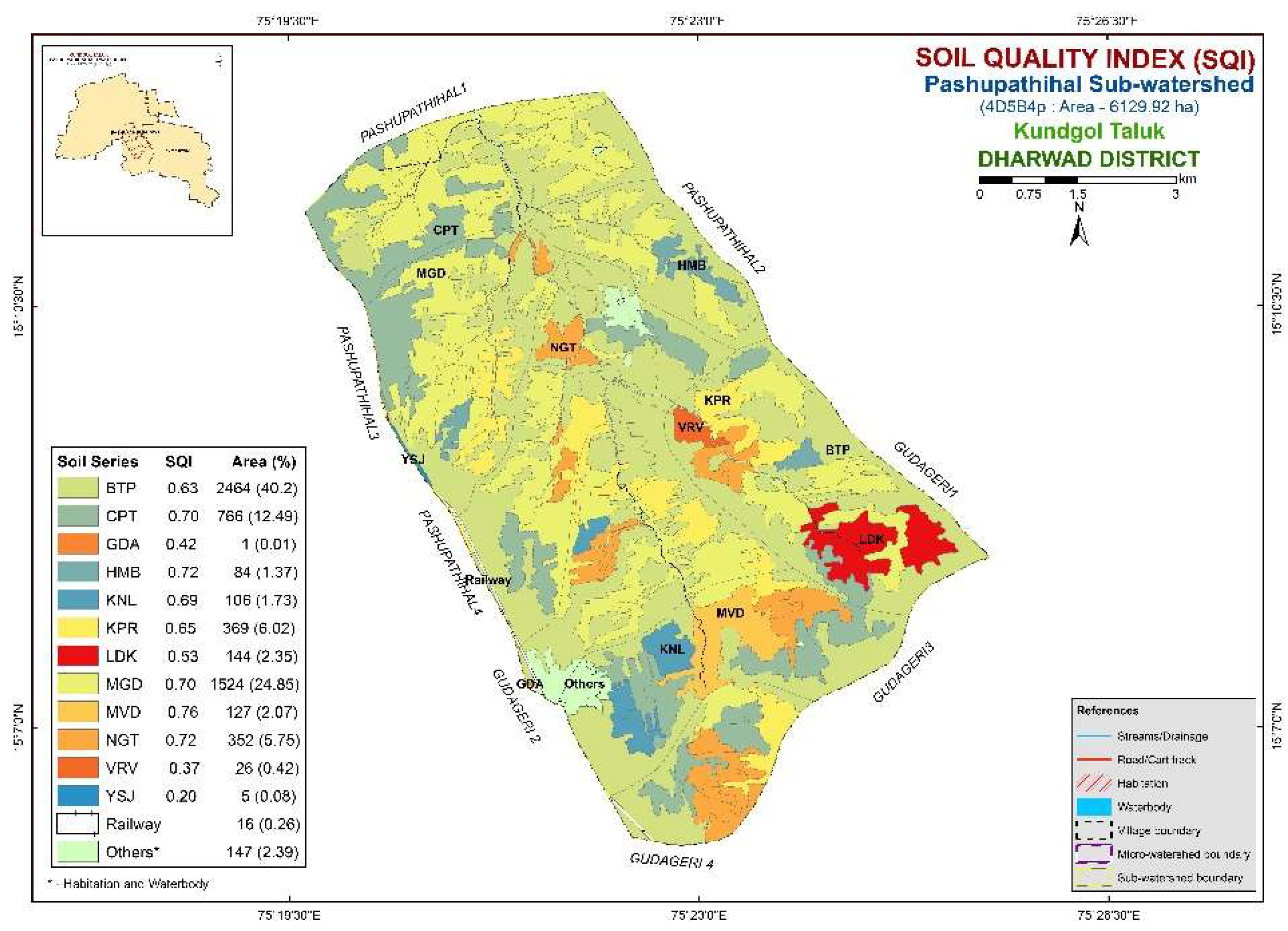

Table 1.
Descriptive statistics of soil properties of soil mapping units used for soil quality index assessment.
Table 1.
Descriptive statistics of soil properties of soil mapping units used for soil quality index assessment.
| Soil parameters | Minimum | Maximum | Mean | Standard Deviation | Kurtosis | Skewness |
|---|---|---|---|---|---|---|
| Depth (cm) | 35.00 | 180.00 | 163.07 | 24.85 | 17.24 | -3.82 |
| CaCO3 (%) | 1.37 | 14.45 | 7.19 | 4.16 | -0.91 | 0.84 |
| pH | 7.01 | 8.96 | 8.70 | 0.34 | 15.70 | -3.72 |
| OC (g/kg) | 2.54 | 6.77 | 3.75 | 0.88 | 4.09 | 1.47 |
| CEC (%) | 21.29 | 56.49 | 49.72 | 6.83 | 8.27 | -2.61 |
| BS (%) | 82.35 | 92.57 | 90.95 | 2.03 | 8.35 | -2.57 |
| EC (dS/m) | 0.16 | 0.43 | 0.27 | 0.06 | -0.40 | 0.33 |
| ESP (%) | 3.17 | 10.17 | 8.32 | 1.29 | 4.75 | -1.23 |
Table 2.
Factors analysis of Bartlett's sphericity test.
| Chi-square (Observed value) | 293.807 |
| Chi-square (Critical value) | 41.337 |
| DF | 28 |
| p-value (Two-tailed) | <0.0001 |
| alpha | 0.05 |
Table 3.
Kaiser-Meyer-Olkin measure of sampling adequacy.
| Depth | 0.652 |
| CaCO3 | 0.434 |
| pH | 0.537 |
| OC | 0.874 |
| CEC | 0.593 |
| BS | 0.807 |
| EC | 0.377 |
| ESP | 0.354 |
| KMO | 0.597 |
Table 4.
Principal Component of Soil mapping units (Soil quality parameters, eigenvalue, components matrix values).
Table 4.
Principal Component of Soil mapping units (Soil quality parameters, eigenvalue, components matrix values).
| Principal Component | PC1 | PC2 | PC3 | PC4 | PC5 | PC6 | PC7 | PC8 |
|---|---|---|---|---|---|---|---|---|
| Eigenvalue | 4.154 | 1.555 | 1.077 | 0.537 | 0.337 | 0.191 | 0.121 | 0.029 |
| Variability (%) | 51.921 | 19.435 | 13.466 | 6.708 | 4.210 | 2.385 | 1.514 | 0.362 |
| Cumulative % | 51.921 | 71.356 | 84.822 | 91.529 | 95.739 | 98.124 | 99.638 | 100.000 |
| Weightage factor | 0.5192 | 0.1944 | 0.1347 | 0.0671 | 0.0421 | 0.0238 | 0.0151 | 0.0036 |
| Factor loadings ( Rotated component matrix) | ||||||||
| Depth | 0.885 | -0.336 | 0.113 | -0.026 | 0.128 | 0.074 | 0.259 | -0.053 |
| CaCO3 | 0.307 | 0.816 | 0.090 | 0.383 | 0.289 | 0.015 | -0.017 | -0.022 |
| pH | 0.887 | 0.286 | 0.257 | 0.053 | -0.194 | -0.069 | 0.079 | 0.121 |
| OC | -0.796 | -0.165 | 0.154 | 0.466 | -0.239 | 0.190 | 0.074 | 0.000 |
| CEC | 0.871 | -0.183 | -0.130 | 0.279 | -0.244 | -0.203 | -0.077 | -0.075 |
| BS | 0.872 | 0.268 | -0.025 | -0.176 | -0.163 | 0.308 | -0.114 | -0.029 |
| EC | 0.230 | -0.495 | 0.813 | 0.054 | 0.140 | 0.010 | -0.135 | 0.004 |
| ESP | 0.533 | -0.562 | -0.536 | 0.239 | 0.193 | 0.090 | -0.070 | 0.068 |
Table 5.
Correlation matrix (Pearson) of soil quality parameters.
| Variables | Depth | CaCO3 | pH | OC | CEC | BS | EC | ESP |
| Depth | 1 | |||||||
| CaCO3 | 0.033 | 1 | ||||||
| pH | 0.7 | 0.488 | 1 | |||||
| OC | -0.641 | -0.254 | -0.65 | 1 | ||||
| CEC | 0.748 | 0.143 | 0.748 | -0.539 | 1 | |||
| BS | 0.657 | 0.378 | 0.832 | -0.736 | 0.653 | 1 | ||
| EC | 0.444 | -0.197 | 0.237 | 0.007 | 0.174 | 0.034 | 1 | |
| ESP | 0.603 | -0.195 | 0.145 | -0.336 | 0.639 | 0.288 | 0.015 | 1 |
Values in bold are different from 0 with a significance level alpha=0.05.
Table 6.
Soil quality index (SQI) values for 46 soil mapping units.
| Sl. No | Soil Mapping Unit | SQI | Sl. No | Soil Mapping Unit | SQI |
|---|---|---|---|---|---|
| 1 | YSJmA1 | 0.20 | 24 | CPTmA2g2Ca | 0.70 |
| 2 | VRVmB2 | 0.37 | 25 | CPTmB2 | 0.70 |
| 3 | HMBmA2g2Ca | 0.72 | 26 | CPTmB2g1Ca | 0.70 |
| 4 | HMBmB2g1Ca | 0.72 | 27 | GDAiA2 | 0.42 |
| 5 | HMBmB2g2Ca | 0.72 | 28 | KNLmA1 | 0.69 |
| 6 | KPRmA1 | 0.65 | 29 | KNLmA2 | 0.69 |
| 7 | KPRmA2g1Ca | 0.65 | 30 | KNLmB2g2Ca | 0.69 |
| 8 | KPRmA2g2Ca | 0.65 | 31 | MGDmA1 | 0.70 |
| 9 | KPRmB2 | 0.65 | 32 | MGDmA1g1Ca | 0.70 |
| 10 | KPRmB2g2Ca | 0.65 | 33 | MGDmA1g2Ca | 0.70 |
| 11 | LDKmA1g1Ca | 0.53 | 34 | MGDmA2g1Ca | 0.70 |
| 12 | LDKmB2g2Ca | 0.53 | 35 | MGDmA2g2Ca | 0.70 |
| 13 | MVDmA2g2Ca | 0.76 | 36 | MGDmB2 | 0.70 |
| 14 | BTPmA1 | 0.63 | 37 | MGDmB2g1Ca | 0.70 |
| 15 | BTPmA1g1Ca | 0.63 | 38 | MGDmB2g2Ca | 0.70 |
| 16 | BTPmA2 | 0.63 | 39 | MGDmB2g3Ca | 0.70 |
| 17 | BTPmA2g1Ca | 0.63 | 40 | NGTmA1 | 0.72 |
| 18 | BTPmB2 | 0.63 | 41 | NGTmA1g1Ca | 0.72 |
| 19 | BTPmB2g1Ca | 0.63 | 42 | NGTmA1g2Ca | 0.72 |
| 20 | CPTmA1 | 0.70 | 43 | NGTmA2g1Ca | 0.72 |
| 21 | CPTmA1g1Ca | 0.70 | 44 | NGTmA2g2Ca | 0.72 |
| 22 | CPTmA1g2Ca | 0.70 | 45 | NGTmB2g1Ca | 0.72 |
| 23 | CPTmA2g1Ca | 0.70 | 46 | NGTmB2g2Ca | 0.72 |
Disclaimer/Publisher’s Note: The statements, opinions and data contained in all publications are solely those of the individual author(s) and contributor(s) and not of MDPI and/or the editor(s). MDPI and/or the editor(s) disclaim responsibility for any injury to people or property resulting from any ideas, methods, instructions or products referred to in the content. |
© 2025 by the authors. Licensee MDPI, Basel, Switzerland. This article is an open access article distributed under the terms and conditions of the Creative Commons Attribution (CC BY) license (http://creativecommons.org/licenses/by/4.0/).
Copyright: This open access article is published under a Creative Commons CC BY 4.0 license, which permit the free download, distribution, and reuse, provided that the author and preprint are cited in any reuse.


