Preprint
Article

This version is not peer-reviewed.

Evaluation of Power System Stability for a Hybrid Power Plant Using Wind Speed and Cloud Distribution Forecasts

A peer-reviewed article of this preprint also exists.

Submitted:

31 January 2025

Posted:

03 February 2025

You are already at the latest version

Abstract

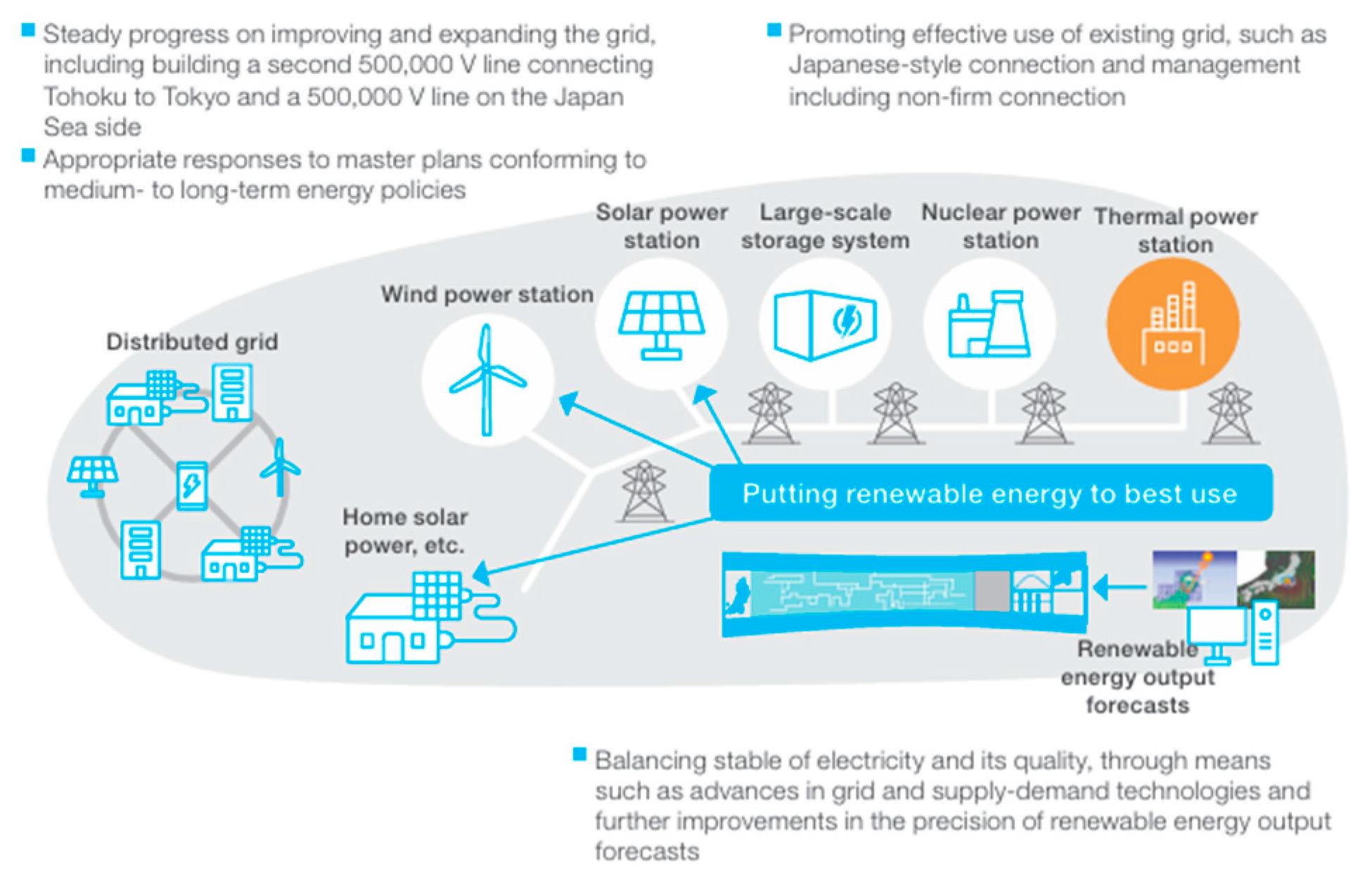
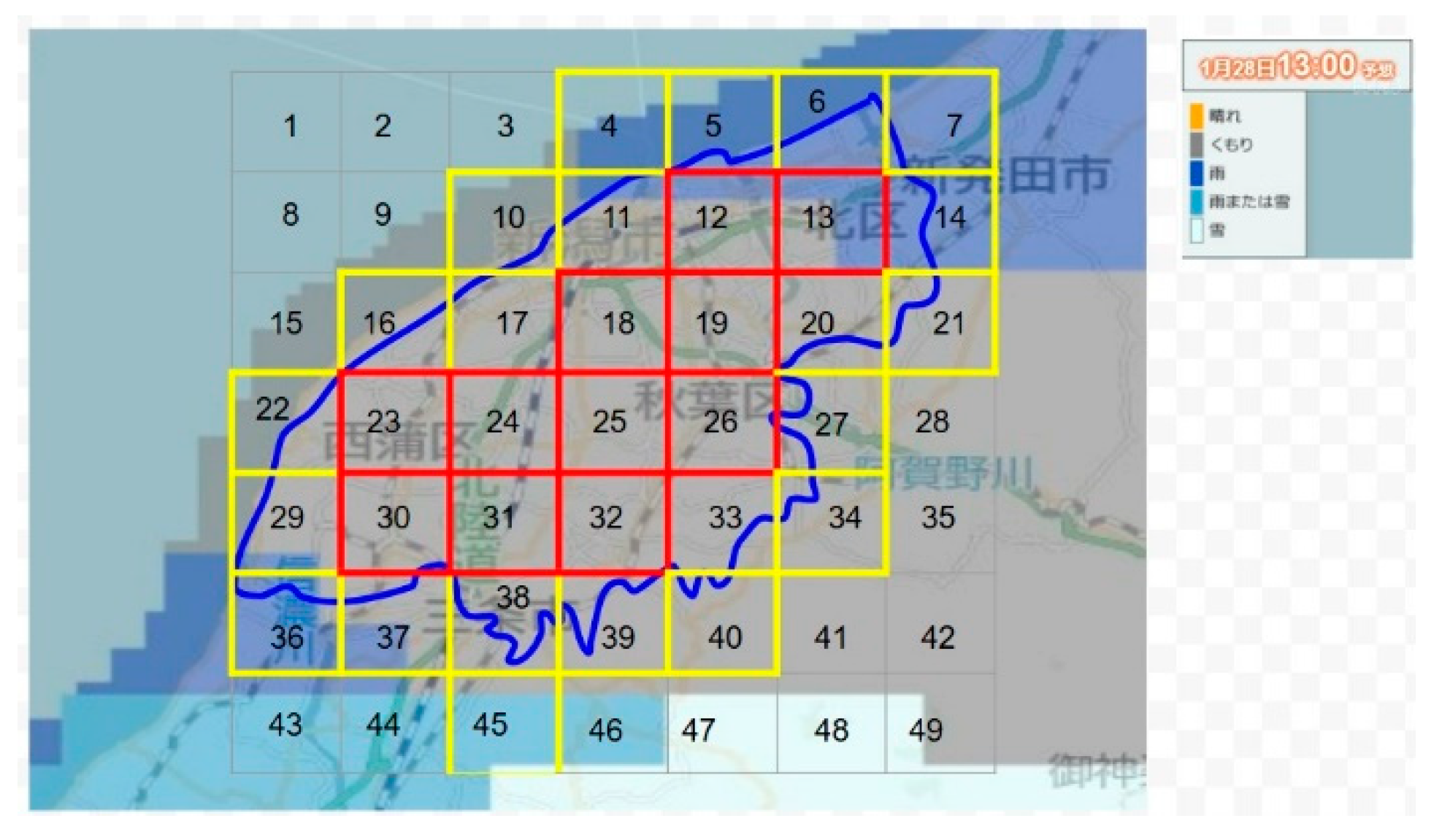
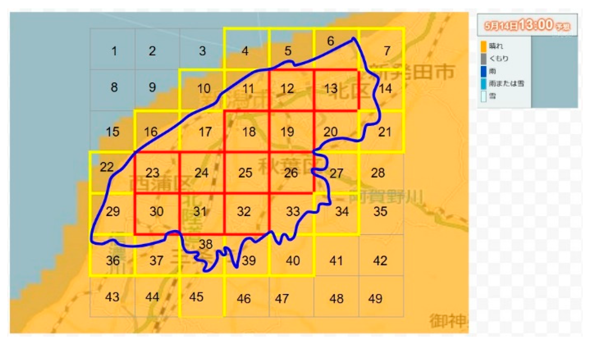
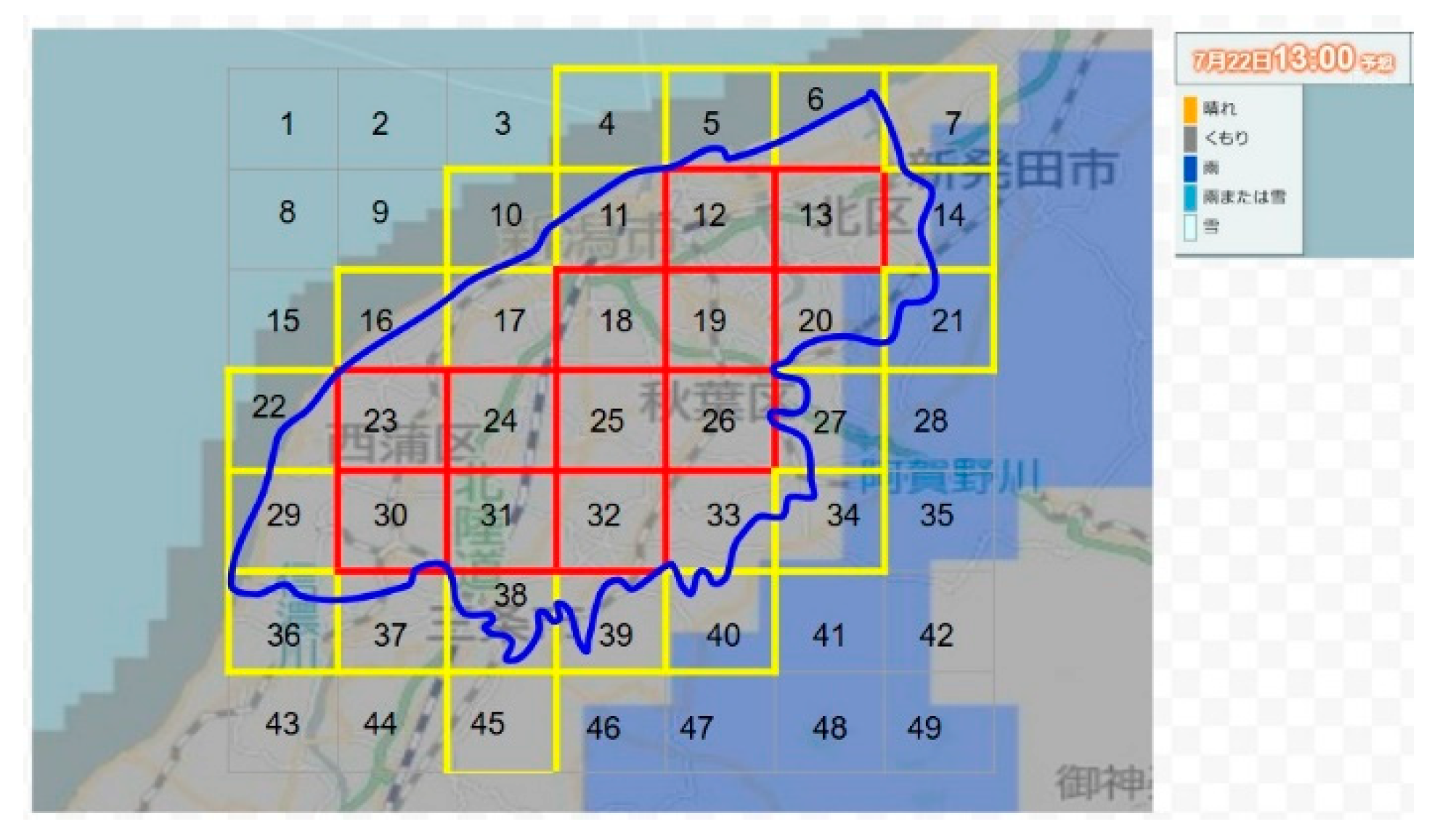
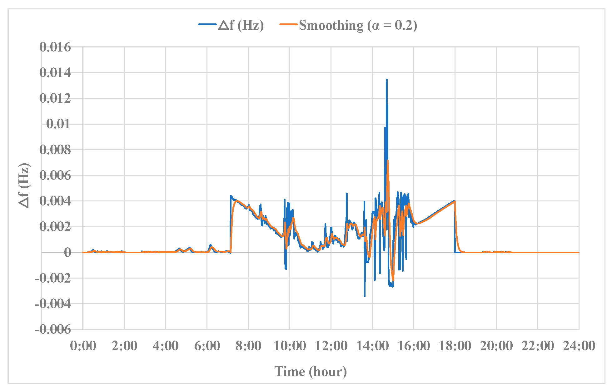
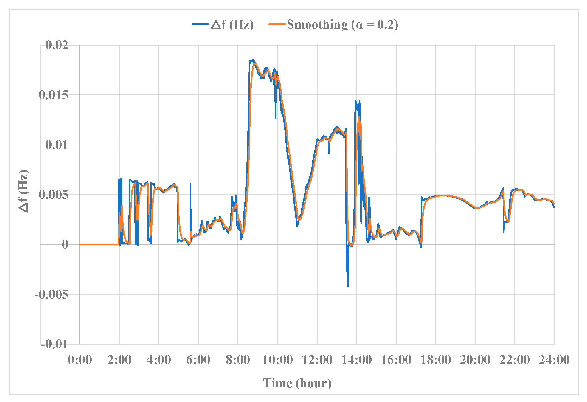
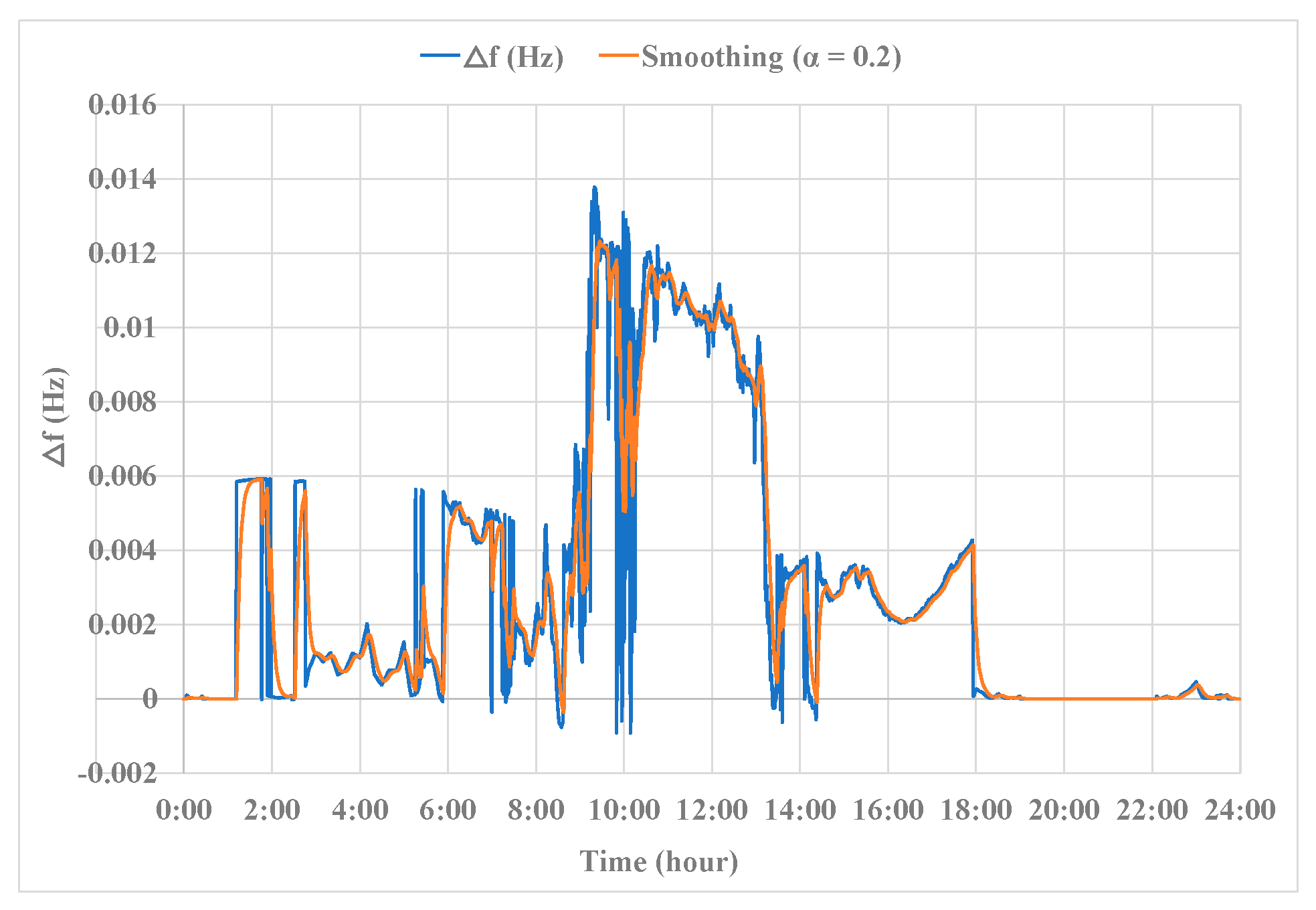
Power system stability (PSS) is the ability of a system to remain in operating equilibrium which is achieved between the electric power generation and consumption. In this paper, we evaluate PSS for a Hybrid power plant (HPP) combining thermal, wind, solar photovoltaic (PV) and, hydro power generations, in Niigata City. A new method to estimate PV power generation, based on NHK cloud distribution forecast (CDF) and land ratio settings, is also introduced. Our objective is to achieve frequency stability (FS) while reducing CO2 emission in the power generation sector. So, PSS is evaluated from the results of the frequency stability (FS) variable. 6-minutes autoregressive wind speed prediction (6ARW) support for wind power (WP). 1-hour GPV wind farm (1HWF) power is computed from the Grid Point Value (GPV) wind speed prediction data. PV power is predicted by autoregressive modelling and CDF. In accordance with the daily power curve and the prediction time, we can support thermal power generation planning. Actual data of wind and solar are measured every 10-minutes and 1-minute, respectively and the hydropower is controlled. The simulation results of the electricity frequency fluctuations are within ±0.2 Hz of the requirements of Tohoku Electric Power Network Co. Inc., for testing and evaluation days. Therefore, the proposed system supplies electricity stably while contributing to CO2 emission reduction.

Keywords: 
;  ;  ;  ;  

1. Introduction

1.1. Background

Variable Renewable Energy (VRE) sources are non-synchronous generation technologies, and this property may require changes to how system stability is ensured, especially during periods of high shares of VRE in power generation[1]. Power system stability (PSS) is the system's ability to maintain a balance between electric power generation and consumption. From its formal definition, Power system stability (PSS) is the ability of an electric power system, for a given initial operating condition, to regain a state of operating equilibrium after being subjected to a physical disturbance, with most system variables bounded so that practically the entire system remains intact[2,3,4]. In line with that, Hatziargyriou et al. (2021) introduced the converter-driven stability and, resonance stability[4]. Then, Shair et al. (2021) proposed a new power system stability (PSS) classification framework which provides wide coverage and future adaptability of the emerging stability issues[5]. Grid stability must be enhanced in light of the integration of large-scale renewable Energy sources into the grid[6]. Also, grid stability must be enhanced considering the integration of large-scale renewable energy sources into the grid[6]. Furthermore, Qin et al. (2022) pointed out that the construction of large-scale renewable energy sources has caused challenges to frequency stability (FS) of power system, and concluded that the influence of factors such as installed locations of renewables and different renewable energy types should be further discussed[7]. The frequency stability (FS) of a power system refers to the ability to maintain a steady frequency when a disturbance is experienced that causes a significant imbalance between generation and demand. Then, Sattar et al. (2024) showed the ability of renewable energy resources and energy storage systems to participate in enhancing frequency stability (FS) through optimal coordination such that the lifetime of the latter does not deteriorate[3]. With renewable energy penetration rate increasing, the system’s frequency stability (FS) will gradually deteriorate, bringing therefore challenges to frequency stability (FS) and security which causes more attention to the analysis method of FS[7]. Besides, the Conference of the Parties (COP) 28 of the United Nations (UN) climate conference underlined the importance of a methodical transition away from fossil fuels to reach net-zero carbon emissions by 2050, with goals of doubling energy efficiency and tripling renewable energy capacity by 2030[8]. So, the need to expedite the energy transition is growing as the strain from climate change increases, making the switch to clean energy an essential alternative[9]. The penetration of more renewable energy into the electrical grid is therefore needed. In fact. the power injected into the grid changes the system operation mode, power flow distribution, and operating points of the traditional equipment, which as a result affects various aspects of classical stability, including power angle, voltage, and frequency stability (FS)[5,10]. As, nuclear and renewable energy are low-carbon energy, it is possible to build sustainable power generation systems that are environmentally friendly. Given that, wind power (WP) and solar photovoltaic (PV) are expected to make a substantial contribution to a more secure and sustainable energy system[1], changes in the design of energy infrastructures should also be considered to support the goal of limiting global warming to 1.5 °C[11]. Bringing into the grid more renewable energy sources is one way to significantly decarbonize electricity[12]. Wei et al. (2022) concluded that CO2 emission reduction will be achieved only with high renewable energy penetration[13]. In line with that, Kosugi et al. (2005)[14] pointed out a model to assess CO2 emission reduction in some energy consuming sectors in Japan and realized that, a scenario where centralized power utilities are combined with decentralized systems is profitable both for consumers and the industry. The new power system that combines conventional and non-conventional power generations as a unit is called a hybrid power plant in this paper. Wind power (WP) and solar photovoltaics (PV) are crucial to meeting future energy needs while decarbonizing the power sector[1]. In February 2024, the Japanese government began issuing Japan Climate Transition Bonds to support their commitment to become carbon neutral by 2050[15]. VRE power plants can provide an increasing proportion of system services (such as frequency and voltage support services), which are relevant to ensuring the reliable operation of the power system. Interestingly, large shares of VRE (up to 45% in annual generation) can be integrated without significantly increasing power system costs in the long run, but each country may need to deal with different circumstances in achieving such a transformation. While the ability to provide such services can increase investment costs for variable renewable energy (VRE) power plants, it can be cost-effective at the system level.[1]. In March 2021, the Tohoku Electric Power Group launched the Tohoku Electric Power Group Carbon Neutral Challenge 2050, from which they want to accelerate CO2 emissions reductions based on maximum use of renewable energy and nuclear power, decarbonization of thermal power sources and, electrification and realization of a smart society. For renewable energy 2,000 MW of new power are to be developed as early as possible by 2030 and thereafter while maintaining and improving the power generation capacity of existing sources[16]. Also, the Feed-in Tariff Scheme for Renewable Energy established by the Japanese Government obliges electric utilities to purchase electricity generated by renewable energy sources at a fixed price for a certain period of time[17]. Diversifying variable renewable resources (VRE) by combining wind, solar photovoltaic, and battery assets in a hybrid power plant (HPP) can increase renewable energy usage efficiency and improve system flexibility, particularly in distributed energy systems[18]. As renewable energy penetrations grow and existing thermal power plants retire, congested regions of both types may increase in prevalence, Kim et al. (2024)[19]. However, many studies on integrating VRE and storage into power grids have not focused on transmission constraints[19,20,21]. Aziz et al. (2018) pointed out that the integration of wind penetration has moved the electricity grid in a transition phase to a new model where wind power plants are expected to participate in all levels of frequency regulation[22]. Ji et al. (2024) concluded that one limitation of their research is the relatively limited energy storage capacity of flywheels compared to some other energy storage technologies. Addressing this limitation is crucial for meeting the prolonged frequency regulation demands of power systems[23]. Hydropower can promote a balanced and diversified energy grid and operate complementary renewable energy generation systems[24,25]. Distributed energy resources (DERs) are elements that actively participate in the supply of renewable energy and contribute to the decarbonization of the power system[26]. Some of the already built infrastructures in hydropower systems could also be used as hidden hydro storage, especially the hydropower plants that are used only seasonally Münch-Alligné et al. (2021)[27,16]. Addressing the research limitation pointed out by Ji et al. (2024) with a hydropower plant set in Niigata city, and given that hybrid power generation system can generate more power than two standalone power plants mainly due to an increase in efficiency[28,18], and in line with the Tohoku Electric Power Group 2050 Carbon Neutral Challenge, along with the related SDG challenges[29], in this paper, a hybrid power plant (HPP) is studied and simulated for Niigata City.

1.2. Objective and Method

Our objective is to evaluate the hybrid power plant (HPP) grid integration based on the frequency stability (FS) variable requirements of Tohoku Electric Power Network Co. Inc. The proposed hybrid power plant (HPP) is a system that combines thermal power generation with wind power, solar photovoltaic (PV) power and, hydropower generations.
In Niigata prefecture the frequency is 50 Hertz and, Figure 1 highlights the distributed grid in the next-generation network[29]. Depending on the geographical location, clouds may affect solar photovoltaic systems grid-connected or standalone. So, we introduce a new mesh method to effectively estimate solar photovoltaic (PV) power generation output of the proposed hybrid power plant (HPP) with a different approach, compared to our previous research[30]. Given that at least 1-year dataset is recommended to evaluate Power system issue, we assume in the simulations, the autumn datasets same as those of spring, due to the similarity of their weather in Niigata City. As weather affects clouds and wind, GPV (Grid Point Value) data provided by the Japan Meteorological Agency (JMA) and calculated with the Global Spectral (GSM) and Meso Scale (MSM) models[31], generate weather maps.
This research is simulated-based under MATLAB, Python, and Excel platforms. In section 2, we predict photovoltaic power. In section 3, the prediction of wind power (WP) is also presented in details, and section 4 is about the power balance along with, the simulation results and discussion. The prediction times are 6-minutes, 1-minute, and 1-hour respectively, for the start-up time of the hydrogenator, the data logger collection time for PV panel at Niigata University and converted actual wind speed data from JMA, and planned power generation of VRE except hydro, respectively. The evaluation of power system stability (PSS) is presented and discussed within ±0.2 Hz of the electricity frequency fluctuations range of Tohoku Electric Power Network Co. Inc., to verify the proposed system’s grid integration.

2. Prediction of Photovoltaic Power

PV power is predicted by autoregressive modelling and CDF. Actual data from a 30 Wp solar photovoltaic panel at Niigata University are measured every minute from a data logger and converted to a PV power plant set at 93 MWp for Niigata City. 6-minutes autoregressive PV power prediction (6ARP) is performed on this measured data using Python. NHK cloud distribution forecast (CDF)[33] data are collected online from the NHK website[33] for 1-hour NHK prediction (1HP) that, contribute to estimate the 93 MWp PV power plant planned power generation. The CDF data are collected from the NHK website every hour, to get a 24 hours CDF image dataset. Basically, under the “mesh” section in the NHK website, 1-hour NHK prediction (1HP) images results are available every hour for 12 hours. From this principle the rest of the CDF data are collected accordingly in 2 or 3 steps to complete the 24 hours dataset. Excel PivotTable converts photovoltaic minutes data to hourly data.

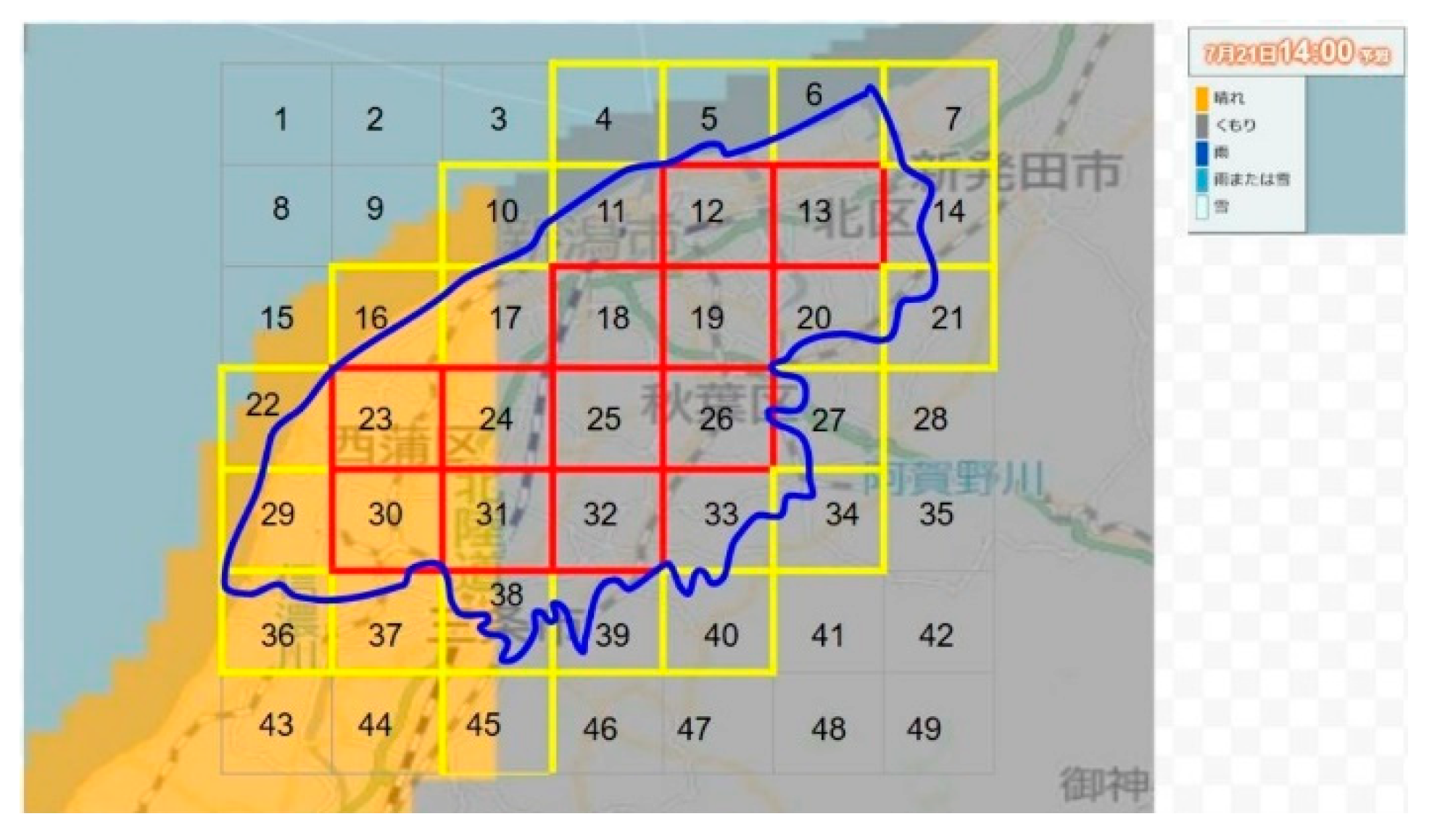
2.1. Mesh Design for PV Power Estimation

In this paper, mesh[34,33] referring to the CDF data is the topology of a network whose components are all connected directly to every other component. Also, it is the number of regular openings per linear inch or centimeters, that are digitally drawn on Google Drawings as shown from Figure 2, Figure 3 and Figure 4. A mesh covers the 726.45 km2 of Niigata City inhabited by 505,272 people in 2024[35], and is put on the NHK cloud distribution forecast (CDF)[33] data in Google Drawings. Figure 2, Figure 3 and Figure 4 show examples for winter, spring, summer, and autumn 2024 at 1 PM. As mentioned in section 1, the dataset of autumn is considered same as those of spring in this paper as a setting. In our previous research[30] we did not set any land distribution ratio based on CDF data like in this research, and even the proposed mesh method is different.
* The picture is taken from the CDF data and Google Maps;
* A mesh is designed on the picture to cover Niigata City.
The scale of the picture is 1:20 km both for the CDF data and Google Maps. Therefore, we can draw in Google Drawings the blue line which represents Niigata City, along with the 7x7 rectangles that form a mesh with the red, yellow, and grey lines as shown in Figure 2, Figure 3 and Figure 4. Each rectangle is identified by a number to complete the entire mesh counted from 1 to 49. The rectangles completely inside the shape of Niigata City are indicated in red while others are in yellow and grey colors. The CDF data with orange, grey, dark blue, clear green and white colors, stand for sunny, cloudy, rainy, rainy with snow, and snowy clouds, respectively.
To get the Photovoltaic estimated power (PVE), each rectangle is set to have both a CDF and land coverage percentage. Supported by NASA (The National Aeronautics and Space administration), NOAA (The National Oceanic and Atmospheric Administration), Table 1 relates power generation with the CDF settings[36,37], while referring to Figure 5, Table 2 elaborates more about the PVE by clarifying in details the land coverage settings. The entire mesh is formed by 49 rectangles represented in column 1 of Table 2, and each rectangle is identified by a number. Furthermore, in column 1, line 2 of Table 2, rectangles 1-3, 8, 9, 15, 28, 35, and 41-49 are, referring to the blue line of Figure 5, not in Niigata City.
Concerning column 2 of Table 2, we set for each rectangle a land distribution ratio based on the CDF data. Assuming that, the inside of the blue line representing the shape of Niigata City is full of land, we can for further illustration purposes, set rectangles 12, 13, 18, 19, 23-26, 31 and 32 land distribution value at 1 each, which means full of land. But, for rectangles 1-3, 8, 9, 15, 28, 35, and 41-49, there is no connection with the blue line meaning that we can set their respective land distribution to 0 which means no land. Then, as the blue line covers parts of rectangles 4 -7, 10-14, 16-27, 29-34, and 36-40, we can accordingly set their land distribution value to 0, 0.17, 0.65, 0.08, 0.15, 0.7, 1, 1, 0.4, 0.4, 0.95, 1, 1, 0.8, 0.2, 0.4, 1, 1, 1, 1, 0.27, 0.75, 0.99, 1, 1, 0.8, 0.1, 0.21, 0.17, 0.56, 0.32, and 0.08, respectively. These values are fixed and not related to the daily weather, time, CDF, or season of the year. Equations 1 and 2 support for the AC solar photovoltaic (PV) generation output by the inverter.
P t ( W ) = 90 100 × 93 × 10 6 × C S P 30 × 1 49 L C I 1 49 R L R
where Pt, is the Alternating Current (AC) solar photovoltaic (PV) generation output by the inverter, and CSP, LCI, RLR stand for Clear Sky Power, Land and Cloud Impacts, and Related Land Ratio, respectively.
L C I = R L R × S A × 1 + C A × 0.3 + R A × 0.1
where SA, CA and RA mean Sunny Cloud Amount, Cloudy Cloud Amount, and Rainy Cloud Amount in Table 1. The ratio of rainy with snow, as well as of snowy clouds are not considered in Equation 2 because a shown in Table 1, their generation capacity is set to zero. Equation 2 is developed to calculate the corresponding land and cloud impacts for every rectangle counted from 1 to 49, and the results are shown in column 3 of Table 2.
Besides, the clear sky data are collected over a period of 24 hours (00 AM-11 PM) and in column 4 of Table 2, we show the temporal clear sky power results. In fact, we have used the Bird model which is a model that estimates clear sky conditions based on the location settings (latitude, longitude, etc.). The clear sky days are assumed for a leap year[38], and for each day of the year, the Bird model provides (in W/m2), data of the direct beam, the direct horizontal irradiance, and of the diffuse horizontal irradiance as well. Among these, the global horizontal irradiance has been used in the current study and it is assumed in the simulations that the maximum irradiance is achieved at the solar panel rated power, i.e. 30Wp at 12 AM, for the winter, spring, and summer cases as we can see from the green curves in Figure 6, Figure 7 and Figure 8. The values presented in column 4 of Table 2 are for the 30 Wp solar panel at Niigata University, but converted to 93 MWp when plotting. After converting, we assume an inverter efficiency of 90 %, to get P t ( W ) . In July 21st, 2024 we obtain P 2 P M M W = 39.1 , as shown in the last line of Table 2. The photovoltaic module type used at a laboratory level of Niigata University is 0.172 m2, model#893TGM500-24V72 for 24 volts rechargeable battery & appliance.
Since we used the Bird model for PV clear sky power estimation at Niigata City[38,30], Figure 6, Figure 7 and Figure 8 highlight in green the clear sky data for the 93Wp PV power plant for the winter, spring, and summer cases, respectively. Then, from Equations 1 and 2, we compute the DC power in Excel., i.e., to get the PVE before the inverter highlighted with red color, and in orange, is the converted measured data from the 30 Wp solar panel of Niigata University.
Due to the influence of temperature on solar panels, the 30 Wp solar panel’s measured value can sometimes be higher than the rated value, which justifies why in Figure 7, the converted measured data, are higher than the clear sky data at 8 and 9 AM. The impact of this error is checked from the simulations results of the electricity frequency fluctuations.

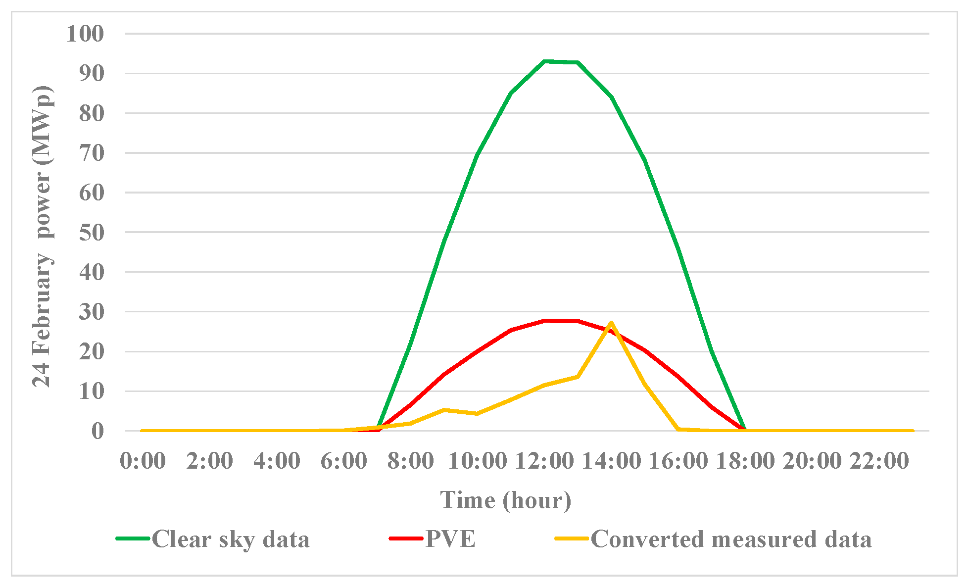
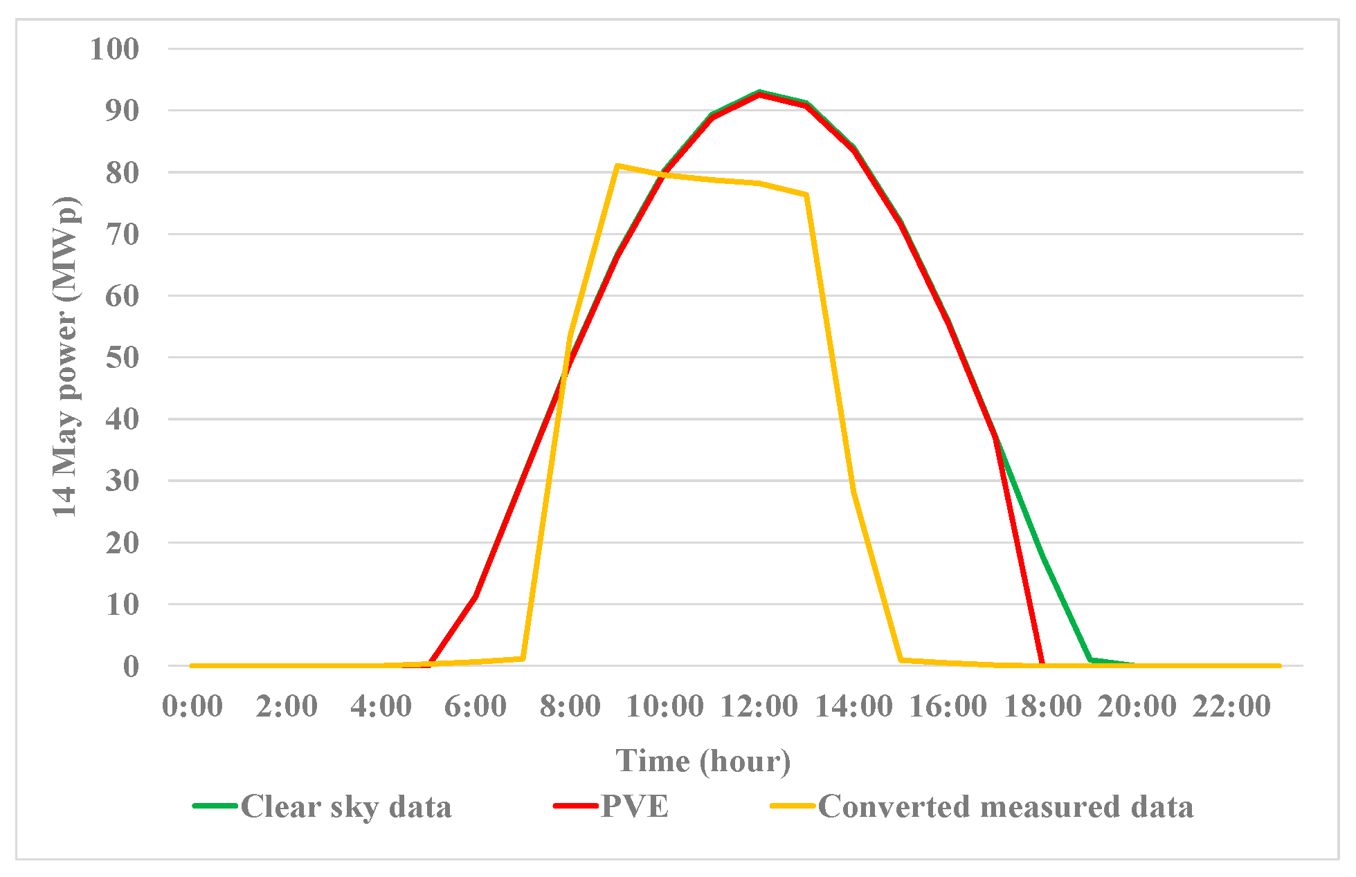
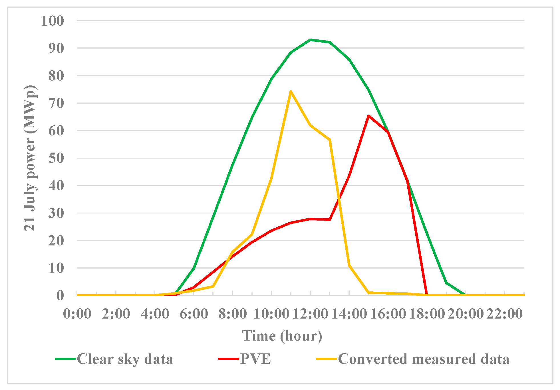
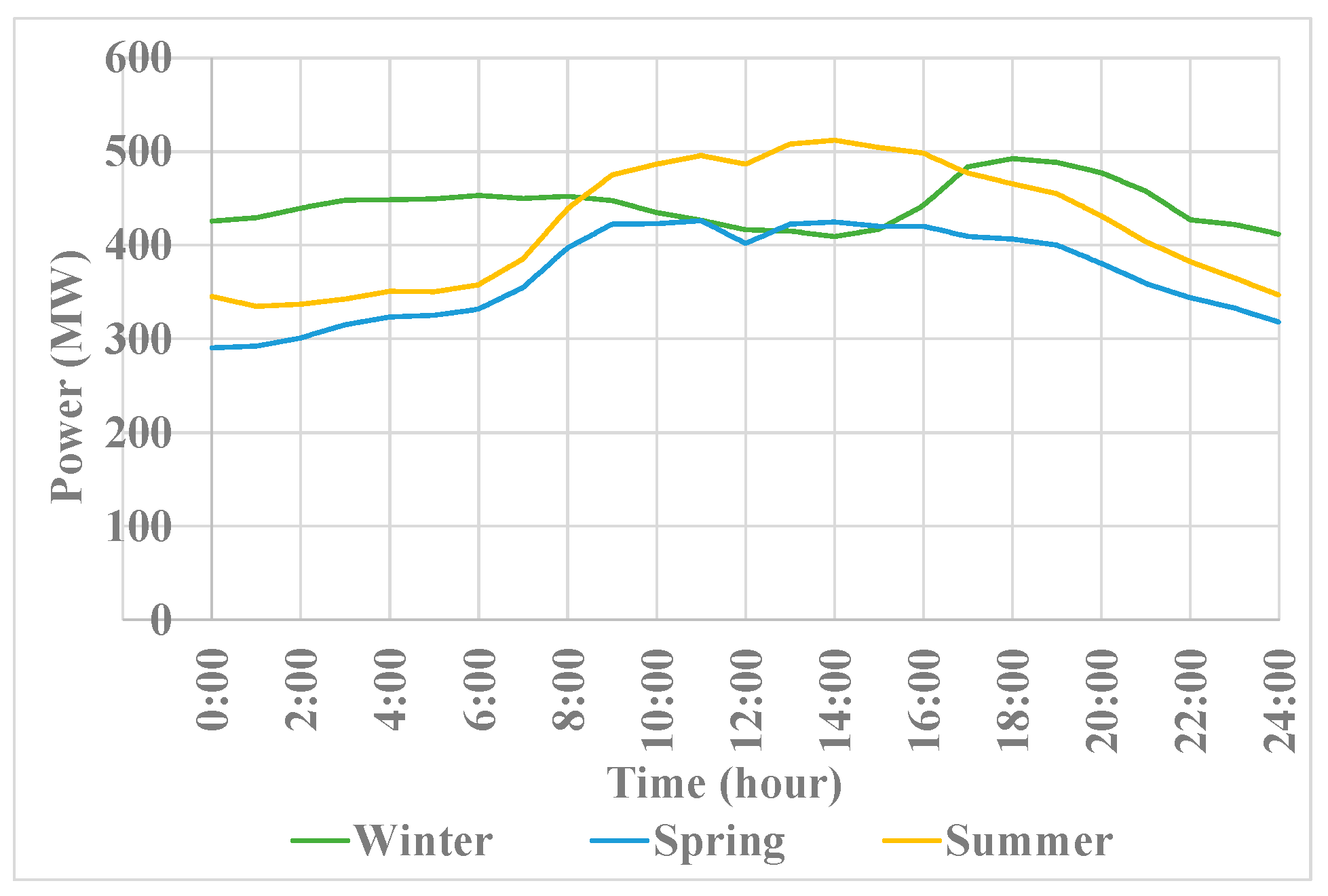
2.2. Niigata City Daily Power Curve

The Tohoku Electric Power Network Co. Inc., supplies 7 prefectures in Japan including Niigata, and Figure 9 highlights the grid settings along with the power stations locations defined in the 2024 Tohoku Electric Power group integrated report[29]. The daily power curve data are available online at the power company webpage, then the value is apportioned to fit the Niigata City population. MATLAB interpolation table converts daily power curve hourly data into 1-minute data by the spline interpolation.
Figure 10 shows the required power at Niigata City on January 28th, May 13th, and July 17th 2024 for the winter, spring, and summer cases.

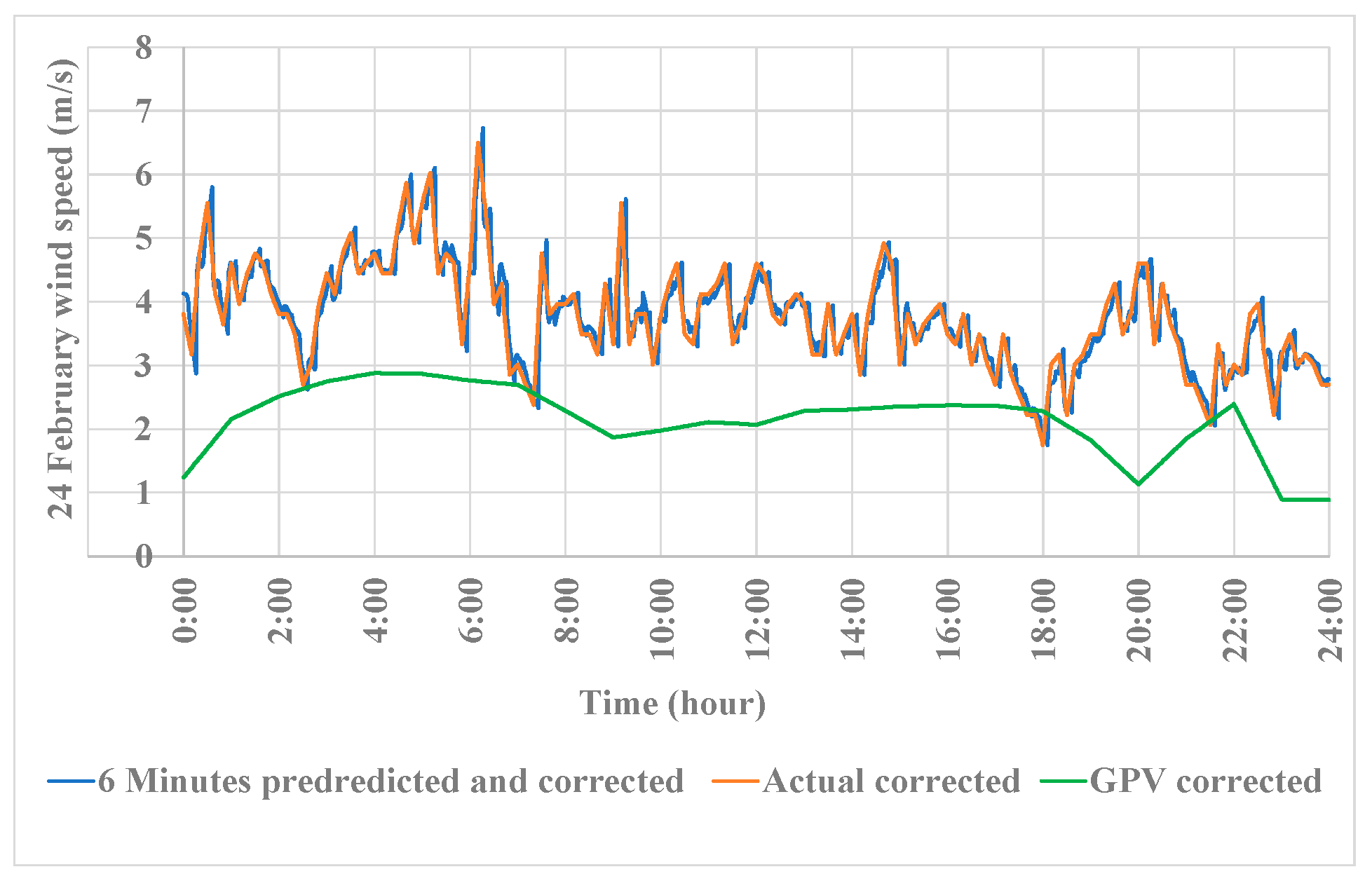
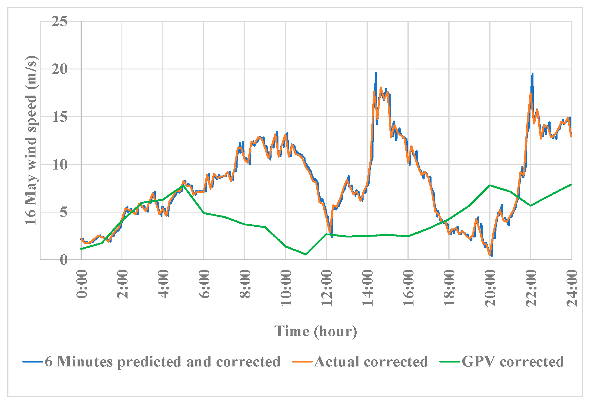
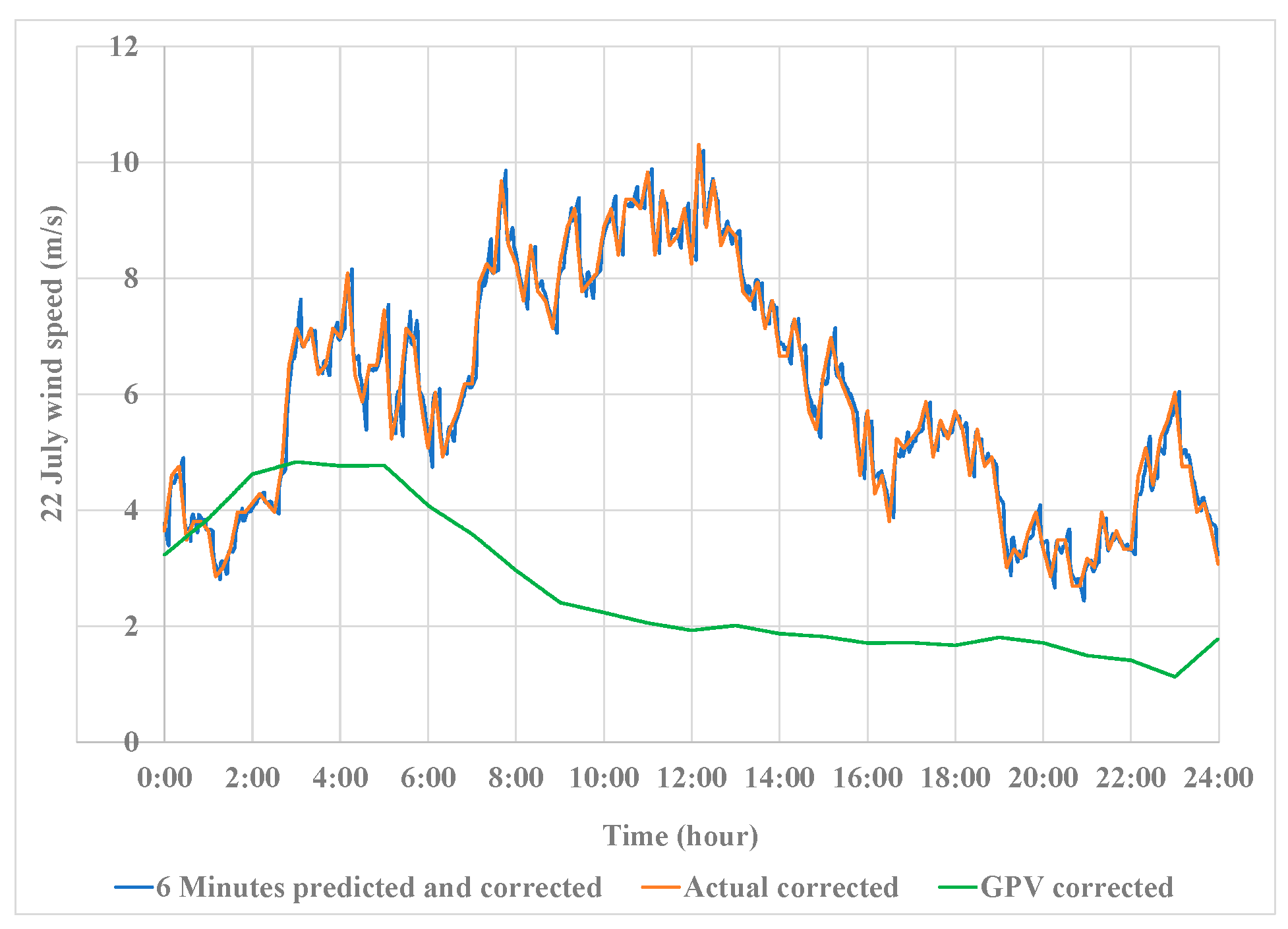
3. Prediction of Wind Power

Wind power is predicted from wind speed, using 6-minutes autoregressive wind speed prediction (6ARW). The 1-hour GPV wind farm (1HWF) is the planned power generation obtained from the GPV wind speed prediction data by Excel computation.
Due to the geographical wind distribution, the output of a wind farm with 10 turbines is not the same as the multiplied output of a single turbine. For example, Figure 11 highlights the wind farm arrangement with lines A and B. The first line includes turbines A1, to A5, which are vertical to the wind direction and, in parallel with line B made by turbines B1 to B5. For example, we assume that the wind observed in line A will reach line B after 2 minutes, and that the distance between these 2 lines is 1km. Similarly, the distance between turbines A1 and A2, is 1 km same as the distance between A2 and A3, A3 and A4, A4 and A5, A1 and B1, B1 and B2, B2 and B3, B3 and B4 and, B4 and B5, as arranged in Figure 11. Furthermore, the power performance of the aerodynamics of double rotor vertical axis wind turbine (VAWT) array is significantly influenced by the relative rotational direction and positioning, ∼8% in power coefficient (CP), while it is marginally dependent on relative phase lag[39]. However, the influence of geographical wind distribution in the calculation of wind farm power is considered as part of the limitations of this paper.
We set testing and evaluation days chosen randomly in all seasons to perform the simulations. The power system control in this research is created by using testing days data and, evaluated by evaluation days data. So, testing day and evaluation days in winter are January 28th, and February 22nd and 24th, respectively. In spring, testing days are May 13th and 15th while evaluation days are May 14th and 16th. Then in summer, July 17th and 21st are the testing days, and July 18th and 22nd, the evaluation days. We set wind farm capacity at 20 MW by combining 2 MW Vestas wind turbines[40]. Basically, the theoretical power available for hydro is calculated with Equation 3, but it is assumed in this research a hydropower capacity (HC) of 20 MW.
P h y d r o ( k W ) = ρ × Q × g × h × η
where P h y d r o , is the theoretical power available, ρ the water density is 1,000 kg/m3, Q the water flow in m3/s, g the acceleration of gravity is 9.81 m/s2, h ( m ) the falling height or head and, η the efficiency usually ranges between 0.75 to 0.95.
The Start-up test results of a vertical-shaft, single-wheel, single-flow Francis Turbine of the Okumen Power Station (rated power 34.5 MW) performed under the jurisdiction of Niigata Enterprises Bureau for reference purposes, show in Table 3, that the starting time of the hydroelectric generator is 347 seconds. From this, a cut-off time of 360 seconds or 6 minutes is set as the starting time of the hydro generator. That is why to prevent lack of electricity generation, we perform 6-minutes autoregressive wind speed prediction (6ARW). MATLAB interpolation table converts wind speed GPV hourly data and, actual wind speed 10-minutes data into 1-minute data by the spline interpolation.
Wind speed is also predicted by autoregressive modelling. In fact, an autoregressive model is a type of time series model that assumes the current value of a variable depends on its previous values. In other words, what happened in the past can give us a clue about what might happen in the future. It is like using historical data to forecast upcoming trends. Autoregressive models (AR) provide valuable insights into time series forecasting by leveraging a variable’s own past values. This simple yet effective approach helps us make informed predictions about future trends and patterns. Autoregressive (AR) models serve as fundamental tools in time series analysis and forecasting, enabling us to make more accurate and data-driven decisions[41].
Figure 12 shows the actual wind speed in Niigata City on February 22nd, May 15th, and July 18th, 2024.
The Japan Meteorological Agency (JMA) provides wind speed data at sea level, and for Niigata city it is 15.1 meters in height[42]. We need to bring the actual and GPV wind speed prediction data to both the site, and Vestas’s wind turbine specifications. We call it wind speed correction in this research in accordance with the Hellmann exponential formula[43], and to perform the correction, Table 4 [44] provides the required coefficients. From the Niigata City topography, we divide the ratio of the sea in the vicinity location by the coast on windward location to obtain the required wind speed ratio to compute the correction. Figure 13, Figure 14 and Figure 15, show the related wind speed predictions together with the GPV wind speed results for the 3 seasons of the year 2024, as examples. The GPV corrected wind speed used to calculated the planned power generation is represented in green while the actual corrected wind speed is represented with the red color.
Since the power system control in this research is created by testing days data and, evaluated by evaluation days data, chosen randomly, the simulations were made for many different days in the same season and are also chosen randomly for presentation in this paper, which explains why the dates in the Figures are sometimes different for the same season of the year.
The wind turbine power curve is highlighted in Figure 16. In fact, by choosing a couple of points (power, wind speed) on the technical datasheet of the Vestas V80-2.0MW wind turbine, we set the polynomial order at 5 in Excel and using the Excel LINEST function, we get -10.151, +836.342, -25696.743, +352324.215, -1909204.441, and 3481877.384, respectively as the equation’s coefficients. By replacing the variable of this polynomial equation with wind speed taken from 0-25 m/s, and computed in an Excel “IF function” with conditions based on the cut-in (4 m/s), rated (16 m/s), and cut-out (25 m/s) wind speeds that are defined in the datasheet, we get the result as shown in Figure 16.

4. Power Balance Simulation

Hydro is added up to 20 MW to get ΔP=0. When hydro power generator is in operation, variable output control with an assumed rate of 10 %/minute is performed[45]. In the case of a shutdown state, it takes 6-minutes to start up, so wind speed prediction after 6-minutes is required, and the system is controlled to eliminate the difference with the daily power curve. We can only increase hydro at a maximum rate of 10 %/min. Figure 17 elaborates more about the power balance.
In Figure 17, AR6 means 6-minutes autoregressive wind farm prediction plus, 6-minutes autoregressive PV power prediction output (6ARP), Plan means 1-hour GPV wind farm (1HWF) plus 1-hour NHK prediction (1HP), then Actual means, Wind farm actual power (WFA) plus photovoltaic estimated power (PVE).
animals or humans, and other studies that require ethical approval, must list the authority that provided approval and the corresponding ethical approval code.

4.1. Simulation Results

From these wind speeds, we can simulate the power generation curves as shown in Figure 18, Figure 19 and Figure 20.
The 6-minutes autoregressive PV power prediction (6ARP) from Python unexpectedly gave 13,814MW at 13:38 PM in Figure 18a, which is very high compared to other power curves values, preventing them to be fully seen. The error might be related to the Python autoregressive model (AR) simulation and its Influence on the frequency stability results is discussed in the latter section. However, by isolating AR6 of Figure 18a, we can obtain Figure 18b showing other power curves in detail.
Equation 4 support the frequency fluctuations of electricity calculation. We set in Excel a curve smoothing factor of 0.2. So, the frequency fluctuation f ( H z ) at the power grid is,
f = P P K
where P ( M W ) represents all the generated output power same as the daily power curve, and P ( M W ) the difference between the predicted photovoltaic and wind farm outputs. Then K ( % M W / H z ) represents the frequency characteristic. Considering the worst-case scenario, we use a K value of 10 in this research. Figure 21, Figure 22 and Figure 23 highlight accordingly the change in the frequency of electricity.

4.2. Results and Discussions

The power system stability of the proposed Hybrid Power Plant (HPP) is evaluated from the frequency stability (FS) simulation results. Tohoku Electric Power Network Co. Inc., provides electricity at 101 V - 50/60 Hz, with permissible limits of ± 6 Volts and ± 0.2 Hz for voltage and frequency fluctuations, respectively. i.e., if the proposed HPP’s simulation results of electricity frequency fluctuations for testing and evaluation days are within these ± 0.2 Hz, power system stability is achieved. The proposed Hybrid Power Plant (HPP) includes a 93 MWp solar photovoltaic (PV) power plant set at Niigata City, a thermal power plant provided by the Tohoku Electric Power Network Co. Inc., through the daily power curve, and a 20 MW wind power plant supported by a 20 MW hydropower plant. After seasonal simulations, we reach the maximum value of +0.013 Hz at 14:42 PM and the minimum value of -0.003 Hz at 13:38 PM in winter, then in spring, a maximum value of +0.018 Hz at 08:46 AM and a minimum value of -0.004 Hz at 13:34 PM. In summer, we get -0.00092 Hz at 10:09 AM as the minimum value and +0.0138 Hz at 09:20 AM for the maximum value, which are all within ±0.2 Hz of the permissible limits of the Tohoku Electric Power Network Co. Inc., and confirm the proposed system grid integration. Despite the error in Figure 18a, the Frequency stability (FS) results are excellent.

5. Conclusions

The simulations results for testing and evaluation days are within ±0.2 Hz as requested by the Tohoku Electric Power Network Co. Inc. So, the proposed Hybrid power plant (HPP) supplies electricity stably to residents of Niigata City, and increases decarbonization. Further to Ji et al. (2024), hydropower is very important in power balance. Renewable energy has successfully shown its relevance in reducing CO2 emission in the power generation sector. The new mesh method based on NHK cloud distribution forecast (CDF) and land ratio settings, has successfully estimated the PV power plant generation output. This with the autoregressive modelling are part of our research benefits. As, some countries are making efforts to reduce the effects of global warming, and given that, it has been pointed out that CO2 emission reduction will not be achieved with short renewable energy grid penetration, this research is clearly in the trend for a sustainable planet. However, in this paper, the following limitations should be addressed in future works. First, a numerical model with mesh size optimization is necessary to improve on the proposed PV output power results. Also, the influence of geographical wind distribution on wind farm power output should be considered in the calculations in future research. The calculation method and results on how much CO2 is reduced from the proposed HPP should be presented in future works, as well.

Author Contributions

Conceptualization, T.D.TCHOKOMANI MOUKAM and A.SUGAWARA; methodology, T.D.TCHOKOMANI MOUKAM and A.SUGAWARA; software, T.D.TCHOKOMANI MOUKAM, Y.LI; validation, T.D.TCHOKOMANI MOUKAM, A.SUGAWARA, Y.BELLO, and Y.LI; formal analysis, A.SUGAWARA, T.D.TCHOKOMANI MOUKAM, Y.LI and Y.BELLO; investigation, T.D.TCHOKOMANI MOUKAM, A.SUGAWARA, Y.BELLO, and Y.LI; resources, T.D.TCHOKOMANI MOUKAM, Y.LI, and Y.BELLO; data curation, T.D.TCHOKOMANI MOUKAM, Y.LI, and Y.BELLO; writing—original draft preparation, T.D.TCHOKOMANI MOUKAM; writing—review and editing, T.D.TCHOKOMANI MOUKAM, A.SUGAWARA, and Y. BELLO; visualization, T.D.TCHOKOMANI MOUKAM, A.SUGAWARA; supervision, A.SUGAWARA; project administration, A.SUGAWARA; funding acquisition, A.SUGAWARA.

Funding

Please add: This research received no external funding.

Data Availability Statement

The original contributions presented in the study are included in the article, the further inquiries can be directed to the corresponding author.

Acknowledgments

The authors are grateful to the Renewable Energy Laboratory of the Faculty of Engineering of Niigata University for providing Laboratory facilities.

Conflicts of Interest

The authors declare no conflict of interest.

Nomenclature

PV Solar photovoltaic;
HC Hydropower capacity;
6ARW 6-minutes autoregressive wind speed prediction;
6ARP 6-minutes autoregressive PV power prediction;
1HWF 1-hour GPV wind farm;
1HP 1-hour NHK prediction;
WFA Wind farm actual power;
PVE Photovoltaic estimated power;
PSS Power system stability;
FS Frequency stability;
HPP Hybrid power plant;
JMA Japan Meteorological Agency;
CDF NHK cloud distribution forecast;
SDG Sustainable development goals;
WP Wind power;
GPV Grid Point Value;
NHK Japan Broadcasting Corporation;
DERs Distributed energy resources;
COP Conference of the parties;
UN United Nations;
VRE Variable renewable energy.

References

  1. International Energy Agency, “The Power of Transformation: Wind, Sun and the Economics of Flexible Power Systems,” IEA (2014) 10 160-179, 2014. https://iea.blob.core.windows.net/assets/b6a02e69-35c6-4367-b342-2acf14fc9b77/The_power_of_Transformation.pdf (accessed Dec. 27, 2024).
  2. V. Chayapathi, S. B, and G. S. Anitha, “Voltage Collapse Mitigation By Reactive Power Compensation At the Load Side,” International Journal of Research in Engineering and Technology, Vol. 02, No. 09, pp. 251–257, 2013. [CrossRef]
  3. F. Sattar, S. Ghosh, Y. J. Isbeih, M. S. El Moursi, A. Al Durra, and T. H. M. El Fouly, “A predictive tool for power system operators to ensure frequency stability for power grids with renewable energy integration,” Applied Energy, Vol. 353, No. PB, p. 122226, 2024. [CrossRef]
  4. N. Hatziargyriou et al., “Definition and Classification of Power System Stability - Revisited & Extended,” IEEE Transactions on Power Systems, Vol. 36, No. 4, pp. 3271–3281, 2021. [CrossRef]
  5. J. Shair, H. Li, J. Hu, and X. Xie, “Power system stability issues, classifications and research prospects in the context of high-penetration of renewables and power electronics,” Renewable and Sustainable Energy Reviews, Vol. 145, 2021. [CrossRef]
  6. C. Chandarahasan and E. S. Percis, “The accessible large-scale renewable energy potential and its projected influence on Tamil Nadu’s grid stability,” Indonesian Journal of Electrical Engineering and Computer Science, Vol. 31, No. 2, pp. 609–616, 2023. [CrossRef]
  7. B. Qin, M. Wang, G. Zhang, and Z. Zhang, “Impact of renewable energy penetration rate on power system frequency stability,” Energy Reports, Vol. 8, pp. 997–1003, 2022. [CrossRef]
  8. A. Rahman, W. M. S.M., M. A.K.M., and X. Wang, “Does renewable energy proactively contribute to mitigating carbon emissions in major fossil fuels consuming countries?,” Journal of Cleaner Production, Vol. 452, pp. 1–16, 2024. [CrossRef]
  9. S. Yuping, S. Shenghu, A. K. Tiwari, S. Khan, and X. Zhao, “Impacts of renewable energy on climate risk: A global perspective for energy transition in a climate adaptation framework,” Applied Energy, Vol. 362, pp. 1–13, 2024. [CrossRef]
  10. HivePower, “Grid Stability Issues With Renewable Energy Sources: How They Can Be Solved,” https://www.hivepower.tech/blog/grid-stability-issues-with-renewable-energy-how-they-can-be-solved (accessed Dec. 06, 2024).
  11. International Energy Agency, “Net Zero by 2050 A Roadmap for the Global Energy Sector.” https://iea.blob.core.windows.net/assets/deebef5d-0c34-4539-9d0c-10b13d840027/NetZeroby2050-ARoadmapfortheGlobalEnergySector_CORR.pdf (accessed Nov. 15, 2024).
  12. M. Arbabzadeh, R. Sioshansi, J. X. Johnson, and G. A. Keoleian, “The role of energy storage in deep decarbonization of electricity production,” Nature Communications, Vol. 10, No. 1, pp. 1–11, 2019. [CrossRef]
  13. L. P. Wei H, Xin L, “TYPES OF CO2 EMISSION REDUCTION TECHNOLOGIES AND FUTURE DEVELOPMENT TRENDS,” Engineering for Rural Development, Vol. 25, 2022. [CrossRef]
  14. T. Kosugi, K. Tokimatsu, and H. Yoshida, “Evaluating new CO2 reduction technologies in Japan up to 2030,” Technological Forecasting and Social Change, Vol. 72, No. 7. pp. 779–797, 2005. [CrossRef]
  15. KIZUNA, “Climate Transition Bonds Show Japan’s Commitment to Carbon Neutrality,” https://www.japan.go.jp/kizuna/2024/09/climate_transition_bonds.html (accessed Dec. 12, 2024).
  16. Tohoku Electric Power Group, “Tohoku Electric Power Group Sustainability report 2023,” https://www.tohoku-epco.co.jp/ir/report/integrated_report/pdf/tohoku_sustainability2023en.pdf#page=15 (accessed Dec. 29, 2024).
  17. Tohoku Electric Power Network Co., “Feed-in Tariff Scheme for Renewable Energy.” https://nw.tohoku-epco.co.jp/consignment/renew/pdf/saisei.pdf (accessed Dec. 26, 2024), (in Japanese).
  18. E. Grant and C. E. Clark, “Hybrid power plants: An effective way ofdecreasing loss-of-load expectation,” Energy, Vol. 307, 2024. [CrossRef]
  19. J. Kim, James Hyungkwan Millstein, Dev Wiser, Ryan Mulvaney-Kemp, “Renewable-battery hybrid power plants in congested electricity markets: Implications for plant configuration,” Renewable Energy, 2024. [CrossRef]
  20. P. Denholm, J. Nunemaker, P. Gagnon, and W. Cole, “The potential for battery energy storage to provide peaking capacity in the United States,” Renewable Energy, Vol. 151, pp. 1269-1277, 2020. [CrossRef]
  21. P. Denholm and T. Mai, “Timescales of energy storage needed for reducing renewable energy curtailment,” Renewable Energy, Vol. 130, 2019. [CrossRef]
  22. A. Aziz, A. T. Oo, and A. Stojcevski, “Analysis of frequency sensitive wind plant penetration effect on load frequency control of hybrid power system,” Electrical Power and Energy Systems, Vol. 99, 2018. [CrossRef]
  23. W. Ji et al., “Applications offlywheel energy storage system on load frequency regulation combined with various power generations: A review,” Renewable Energy, 2024. [CrossRef]
  24. C. Kennedy, D. Bertram, and C. J. White, “Reviewing the UK’s exploited hydropower resource (onshore and offshore),” Renewable and Sustainable Energy Reviews, 2024. [CrossRef]
  25. J. E. Sample, N. Duncan, M. Ferguson, and S. Cooksley, “Scotland’s hydropower: Current capacity, future potential and the possible impacts of climate change,” Renewable and Sustainable Energy Reviews, 2015. [CrossRef]
  26. J. C. Sarmiento-Vintimilla, D. M. Larruskain, E. Torres, and O. Abarrategi, “Assessment of the operational flexibility of virtual power plants to facilitate the integration of distributed energy resources and decision-making under uncertainty,” International Journal of Electrical Power and Energy Systems, 2024. [CrossRef]
  27. V. Karapici et al., “Opportunities of hidden hydropower technologies towards the energy transition,” Energy Reports, 2024. [CrossRef]
  28. C. Zhou, E. Doroodchi, and B. Moghtaderi, “Figure of Merit Analysis of a Hybrid Solar-Geothermal Power Plant,” Engineering, Vol. 5, No. 1, doi: doi:10.4236/eng.2013.51b005.
  29. TOHOKU ELECTRIC POWER GROUP, “Tohoku Electric Power Group Integrated Report 2024,” 2024. https://www.tohoku-epco.co.jp/ir/report/integrated_report/pdf/tohoku_integratedreport2024en.pdf (accessed Dec. 29, 2024).
  30. T. D. TCHOKOMANI MOUKAM, A. SUGAWARA, I. L. SHAWAPALA, Y. BELLO and Y. LI, Stabilization of Electricity by Mesh Method and Combination of Renewable Energy System, The International Council on Electrical Engineering Conference2024, 0-060,June 2024 Kitakyushu, Japan.
  31. “JMA/GPV Weather Maps,” 2024. https://www.basso-continuo.com/WeatherGPV/index_e.htm (accessed Dec. 30, 2024).
  32. Agora Energiewende, “Integrating renewables into the Japanese power grid by 2030,” 148/1-S-2019/EN. https://www.renewable-ei.org/pdfdownload/activities/REI_Agora_Japan_grid_study_FullReport_EN_WEB.pdf (accessed Jan. 30, 2025).
  33. NHK (Japan Broadcasting Corporation), “NHK News web,” 2024. https://www.nhk.or.jp/kishou-saigai/city/status/15100001510700/ (accessed Dec. 30, 2024).
  34. Vocabulary.com, “Mesh,” 2024. https://www.vocabulary.com/dictionary/mesh (accessed Dec. 30, 2024).
  35. “Population of Cities in Japan 2024,” 2024. https://worldpopulationreview.com/cities/japan%0A%0A (accessed Oct. 25, 2024).
  36. “Introduction to clouds.” https://www.ncei.noaa.gov/sites/default/files/sky-watcher-cloud-chart-noaa-nasa-english-version.pdf (accessed Feb. 09, 2024).
  37. X. Zhu, J. Yan, and N. Lu, “A Graphical Performance-Based Energy Storage Capacity Sizing Method for High Solar Penetration Residential Feeders,” IEEE Transactions on Smart Grid, Vol. 8, No. 1, 2017. [CrossRef]
  38. T. P. S. U. Jeffrey Brownson, College of Earth and Mineral Sciences, “Clear Sky Model and Measured Irradiance Data,” 2023. https://www.e-education.psu.edu/eme810/node/698 (accessed Mar. 20, 2024).
  39. S. Sahebzadeh, A. Rezaeiha, and H. Montazeri, “Vertical-axis wind-turbine farm design: Impact ofrotor setting and relative arrangement on aerodynamic performance ofdouble rotor arrays,” Energy Reports, Vol. 8, 2022. [CrossRef]
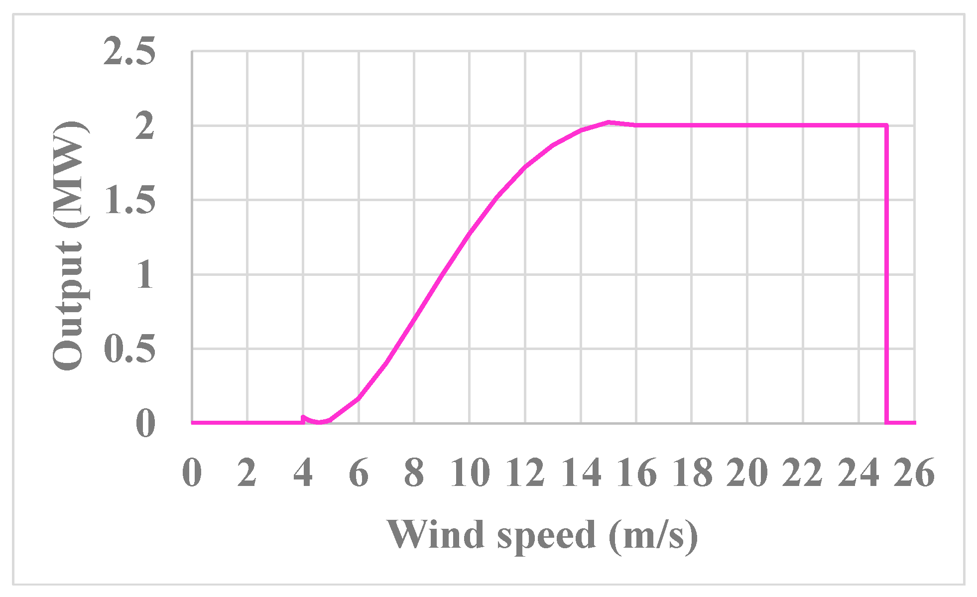
  40. Vestas, “Vestas V80-2.0 MW, Facts and figures,” 2011. https://www.ledsjovind.se/tolvmanstegen/Vestas V90-2MW.pdf (accessed Feb. 19, 2024).
  41. J. Chaudhari, “Understanding Autoregressive (AR) Models for Time Series Forecasting,” Jul 25, 2023, 2023. https://jaichaudhari.medium.com/understanding-autoregressive-ar-models-for-time-series-forecasting-508016498a1e (accessed Dec. 31, 2024).
  42. J. M. Agency, “JMA Height for Niigata (in Japanese),” 2024. https://www.jma-net.go.jp/niigata/gaikyo/geppo/kishou_ichiran.pdf.
  43. F. Bañuelos-Ruedas, C. Á. Camacho, and S. Rios-Marcuello, “Methodologies Used in the Extrapolation of Wind Speed Data at Different Heights and Its Impact in the Wind Energy Resource Assessment in a Region,” Wind Farm - Technical Regulations, Potential Estimation and Siting Assessment, p. 100, 2011. [CrossRef]
  44. A. Hiroshi, K. Yasutsugu, and I. Meng, “A method for estimating offshore winds using a three-dimensional wind model,” Japan Society of Civil Engineers (in Japanese), Vol. 54, p. 134, 2007, [Online]. Available: http://library.jsce.or.jp/jsce/open/00008/2007/54-0131.pdf, accessed date is october 13th, 2023.
  45. H. Glattfelder, L. Huser, P. Dörfler, and J. Steinbach, “Automatic Control for Hydroelectric Power Plants,” Encyclopedia of Life Support Systems (EOLSS), Vol. XVIII. [Online]. Available: https://www.eolss.net/Sample-Chapters/C18/E6-43-33-04.pdf (accessed Oct. 25, 2023).
Figure 1. Next-generation network with distributed grid[29,32].
Preprints 147848 g001
Figure 2. Mesh on CDF data (28/Jan/2024).
Preprints 147848 g002
Figure 3. Mesh on CDF data (14/May/2024).
Preprints 147848 g003
Figure 4. Mesh on CDF data (22/July/2024).
Preprints 147848 g004
Figure 5. Mesh on CDF data (21/Jul./2024).
Preprints 147848 g005
Figure 6. Power of the 93 MWp PV plant (24/Feb./2024).
Preprints 147848 g006
Figure 7. Power of the 93 MWp PV plant (14/May/2024).
Preprints 147848 g007
Figure 8. Power of the 93 MWp PV plant (21/Jul/2024).
Preprints 147848 g008
Figure 9. Grid specifications and power station locations[29,32].
Preprints 147848 g009
Figure 10. Daily power curves.
Preprints 147848 g010
Figure 11. Arrangement example of the wind farm.
Preprints 147848 g011
Figure 12. Actual wind speeds.
Preprints 147848 g012
Figure 13. Wind speed forecasts (24/Feb./2024).
Preprints 147848 g013
Figure 14. Wind speed forecasts (16/May/2024).
Preprints 147848 g014
Figure 15. Wind speed forecasts (22/Jul./2024).
Preprints 147848 g015
Figure 16. Wind turbine power curve[40].
Preprints 147848 g016
Figure 17. Power balance flow chart.
Preprints 147848 g017
Figure 18. Power generation change example (24/Feb./2024).
Preprints 147848 g018
Figure 19. Power generation change example (16/May/2024).
Preprints 147848 g019
Figure 20. Power generation change example (22/Jul./2024).
Preprints 147848 g020
Figure 21. Frequency fluctuation example (24/Feb./2024).
Preprints 147848 g021
Figure 22. Frequency fluctuation example (16/May/2024).
Preprints 147848 g022
Figure 23. Frequency fluctuation example (22/Jul./2024).
Preprints 147848 g023
Table 1. Settings on clouds and power.
Coverage type Amount Generating power
Sunny 0 1
Cloudy 0.7 0.3
Rainy 0.9 0.1
Rainy with snow 1 0
Snowy 1 0
Table 2. Power estimation method.
Rectangles (1-49) Related land ratio Land and cloud Impacts Temporal clear sky power (Wp)
1-3, 8, 9, 15, 28, 35, 41-49 0 0 0
4 0 0 0
5 0.17 0.04539 0
6 0.65 0.195 0
7 0.08 0.024 0
10 0.15 0.07875 0
11 0.7 0.21 3.139
12 1 0.3 9.202
13 1 0.3 15.327
14 0.4 0.12 20.884
16 0.4 0.4 25.402
17 0.95 0.6175 28.521
18 1 0.3 30
19 1 0.3 29.7254
20 0.8 0.24 27.72
21 0.2 0.06 24.132
22 0.4 0.34 19.25
23 1 1 13.46
24 1 0.65 7.273
25 1 0.3 1.463
26 1 0.3 0
27 0.27 0.081 0
29 0.75 0.75 0
30 0.99 0.99 0
31 1 0.65
32 1 0.3
33 0.8 0.24
34 0.1 0.03
36 0.21 0.21
37 0.17 0.17
38 0.56 0.364
39 0.32 0.096
40 0.08 0.024
P 2 P M M W 39.1
Table 3. Starting characteristics of hydro generators.
Time since start-up operation (s)
To the end of bypass valve opening 21
Until the end of the main valve opening 156
Waterwheel start-up 160
Up to excitation 206
Until the automatic synchronization system
is activated
233
Up to synchronous parallelism 245
Up to a given load 347
Table 4. Carruthers wind speed ratios[44].
Location Ratio
On the sea 0.60
Low-lying Island 0.55
Coast on windward side, low land in the vicinity 0.50
Downwind side of the coast, low land, or sea in the vicinity 0.40
Open land with few obstructions 0.40
Shielded land and cities 0.30
Disclaimer/Publisher’s Note: The statements, opinions and data contained in all publications are solely those of the individual author(s) and contributor(s) and not of MDPI and/or the editor(s). MDPI and/or the editor(s) disclaim responsibility for any injury to people or property resulting from any ideas, methods, instructions, or products referred to in the content.
Copyright: This open access article is published under a Creative Commons CC BY 4.0 license, which permit the free download, distribution, and reuse, provided that the author and preprint are cited in any reuse.
Prerpints.org logo

Preprints.org is a free preprint server supported by MDPI in Basel, Switzerland.

Subscribe

Disclaimer

Terms of Use

Privacy Policy

Privacy Settings

© 2025 MDPI (Basel, Switzerland) unless otherwise stated