1. Introduction
Brazil is a global leader in sugarcane production, consistently ranking as the world’s largest producer. In 2022, around 724 million tons of sugarcane were produced in the country, remaining ahead of India (439 million tons) and China (103 million tons) [
12]. This strategic crop is a cornerstone of the Brazilian agricultural sector, contributing significantly to ethanol and sugar production. The continuous adoption of advanced technologies by Brazilian farmers and industries of the sugar and alcohol sector has played a crucial role in maintaining this leadership position, even in the face of recent climatic challenges scenarios [
23].
Among these technologies, images obtained from remote sensing have been gaining prominence in recent years, mainly due to the increasing availability of multispectral images with high temporal and spatial resolution. Therefore, obtaining recurrent maps of vegetation indices throughout all crop phenological stages contributes substantially to developing increasingly accurate yield estimation models [
2].
On the other hand, it is essential to recognize that data collected in field experiments are often conditioned to external factors that can impact sugarcane productivity. Examples include agricultural management, water availability, climatic conditions, and the incidence of pests and diseases. Due to these influences, such data often exhibit heteroskedastic behavior, i.e., non-constant variance, necessitating the application of appropriate statistical techniques. For instance, Prataviera et al. [
29] proposed a log-Weibull regression model for interval-censored data, incorporating a regression structure for the location (
) and scale (
) parameters, enabling the modeling of non-proportional hazards and heteroskedasticity, one application of this model involved analyzing the effects of different treatments in dairy cows, where significant differences among treatments were observed. Similarly, Santos et al. [
35] evaluated the impact of
Bacillus inoculants on sugarcane using a heteroskedastic semiparametric GA regression model. The model predicted significant productivity increases and confirmed the efficacy of the inoculant in reducing the use of phosphate fertilizers. Vasconcelos et al. [
43] proposed a heteroskedastic regression model to analyze the effects of temperature and wood species on shrinkage volume.
Furthermore, when vegetation indices originating from satellite images are used in addition to field data, a significant increase in the dimensionality of the data set is commonly observed, given the number of indices available in the literature that can be potential indicators of biomass accumulation and physiological development. In this context, supervised machine learning (ML) techniques, capable of performing multivariate analyses with high precision, have been widely used in the literature to support the development of yield estimation models [
26,
36]. While artificial neural networks (ANN) were the first computational models that introduced the ML concepts and were inspired by the biological neural networks of the human brain [
21], the multilayer perceptrons (MLPs) are a type of ANN with one or more hidden layers that allow them to learn complex patterns in the data. MLPs are widely used for various tasks (including regression) due to their ability to fit any continuous function [
41]. Another widely used type of ML algorithm is decision trees [
19]. However, with the increasing complexity of the data used to generate regression models, isolated trees have become insufficient, leading to more robust techniques, such as the Random Forest (RF) [
5] that operates by building a multitude of decision trees during training. This process involves randomly selecting subsets of data and features to train each tree, reducing overfitting and improving generalization.
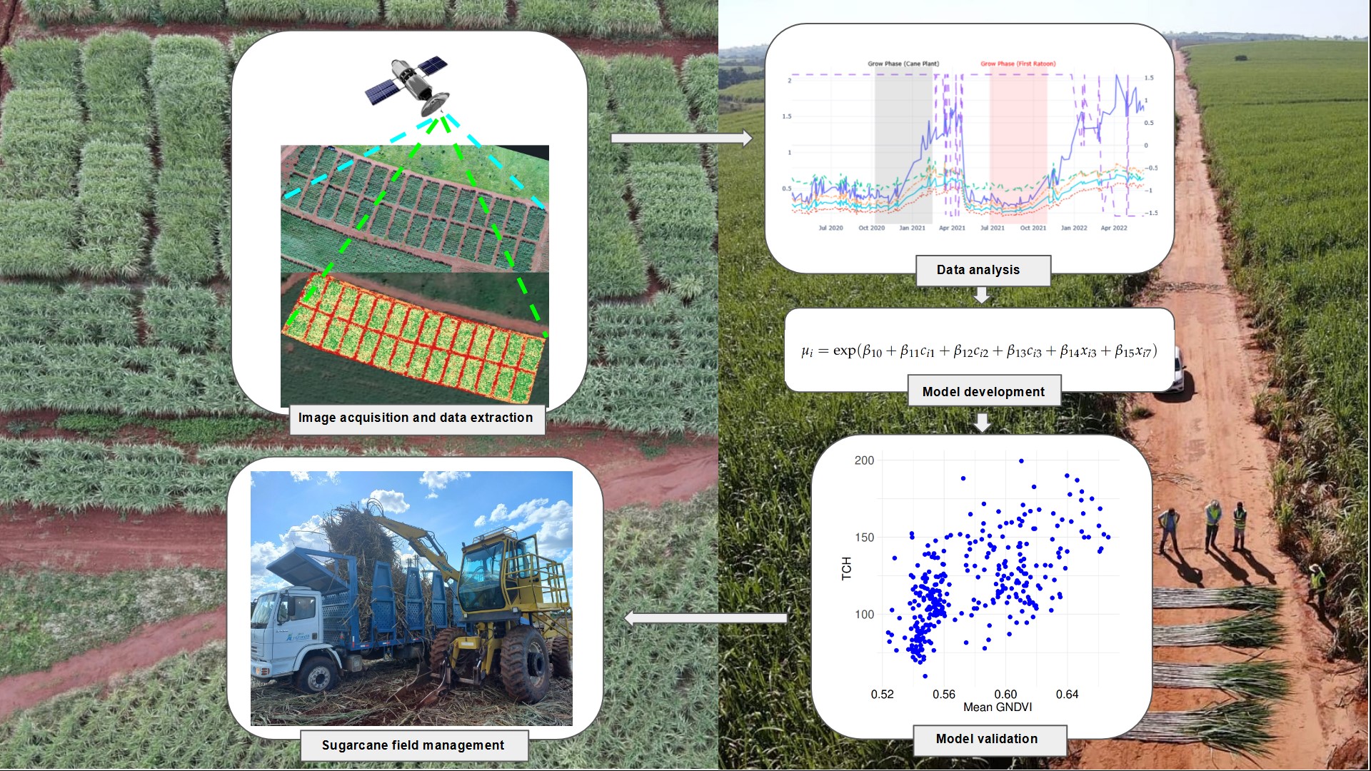
This work aimed to evaluate the feasibility of using time series analysis from satellite images to monitor the development of two experimental sugarcane fields during two growth cycles. Its goal was to verify the efficiency and accuracy of yield estimation generated by different models using this data set.
2. Materials and Methods
2.1. Field Experiment Methodology
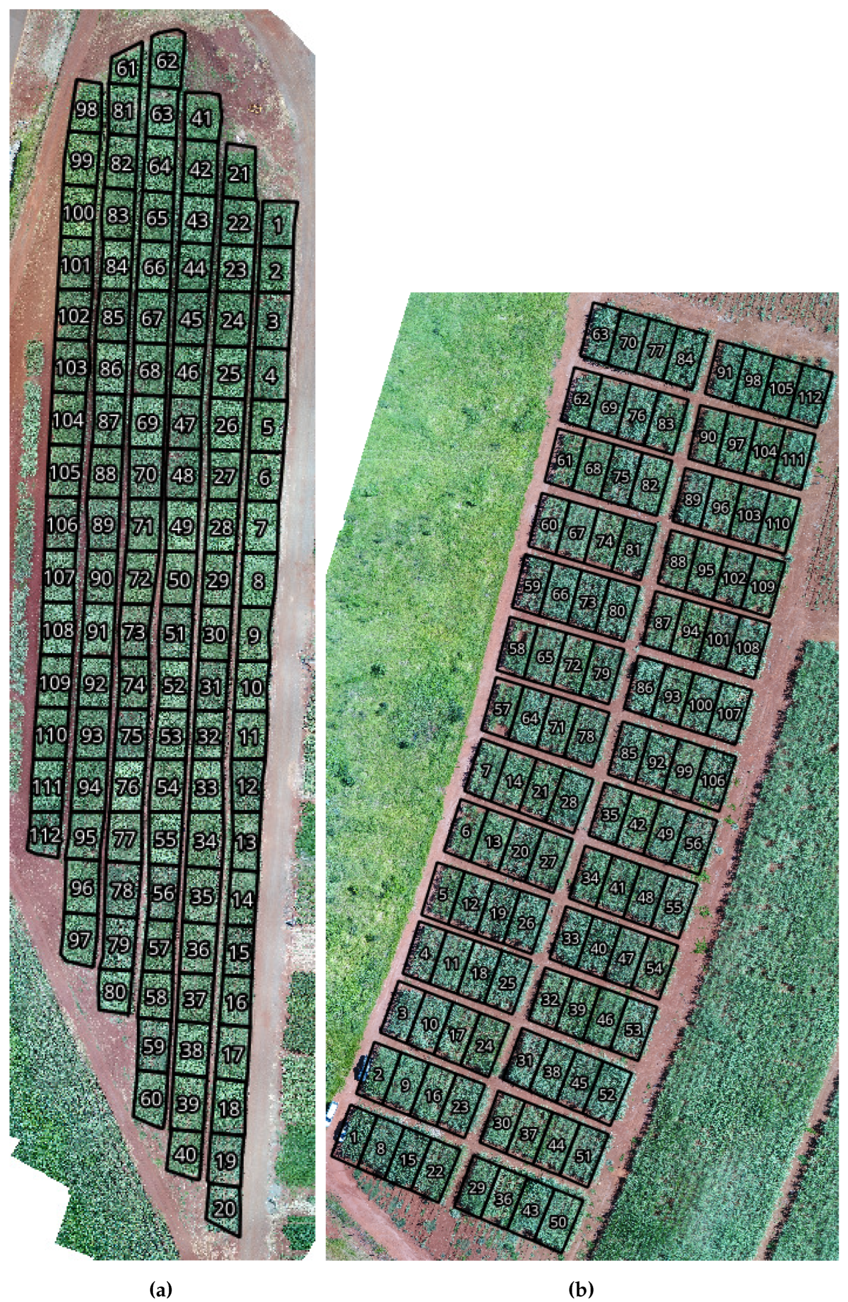
This study was carried out with four sugarcane varieties cultivated in two distinct locations during the growth seasons of 2020/2021 and 2021/2022. The sugarcane varieties were selected based on the length of the growth cycle (see Table 1). Each experimental field consisted of 112 plots with six rows of sugarcane measuring 1.5 m between furrows and 10 m in length (Figure 1). For each sugarcane variety, there were 28 replicates per experimental field, totaling 448 experimental plots.
Table 1.
Sugarcane varieties identification and and the respective length of growth cycle.
Table 1.
Sugarcane varieties identification and and the respective length of growth cycle.
| Sugarcane Varieties |
Cycle |
| CTC1007 (V1) |
Normal |
| RB966928 (V2) |
Short |
| CV0618 (V3) |
Medium |
| CV7870 (V4) |
Normal |
Both experiments had two production cycles, one for the cane plant cycle (2020/2021) and the other for the first ratoon cycle (2021/2022).
The experimental site located in the rural area of Piracicaba, São Paulo, Brazil (-22.773005, -47.580135), utilized two-month-old pre-sprouted seedlings (PSS) that were initially cultivated in a greenhouse for each variety. A drip irrigation system was implemented during the first three months after transplanting the plantlets into the field to promote robust root development. In contrast, the experimental site in the rural area of Tambaú, São Paulo, Brazil (-21.708543, -47.246643), employed sugarcane stalks with an average length of 1.5 meters as plantlets for direct field planting. Both experimental sites followed management practices aligned with standard commercial sugarcane cultivation in Brazil, ensuring consistent agronomic standards across all varieties.
Figure 1.
Aerial perspective of experimental fields (a) and (b), highlighting the 112 plots in each field. Where (a) is the experimental field located in Piracicaba, Sao Paulo, Brazil; and (b) is the experimental field located in Tambau, Sao Paulo, Brazil.
Figure 1.
Aerial perspective of experimental fields (a) and (b), highlighting the 112 plots in each field. Where (a) is the experimental field located in Piracicaba, Sao Paulo, Brazil; and (b) is the experimental field located in Tambau, Sao Paulo, Brazil.
Sugarcane plots were harvested and measured as tons of cane per hectare (TCH, t ) at the end of its growth cycle once the stalks reached peak maturity, determined by measuring the total recoverable sugars (TRS) concentration. Productivity was assessed based on the average stalk weight obtained from experimental replicates for each treatment across all locations (Piracicaba and Tambaú) over two consecutive harvest cycles (2020/2021 and 2021/2022).
2.2. Commercial Area Data
To assess the effectiveness of the models under real environment of sugarcane production, 12 commercial sugarcane plots cultivated in the state of São Paulo, Brazil, were analyzed during the growing season of 2022. These plots had known observed productivity data, which were used to compare with the results generated by the models. Detailed productivity metrics, sugarcane cycle, varieties and geographic coordinates of the commercial plots are provided in Table 7 of the Supplementary Data.
2.3. Vegetation Indices
A vegetation index is an algebraic combination of various spectral bands designed to highlight the vigor and properties of vegetation [
38]. It translates information contained in multispectral or RGB images through linear transformations of reflectance factors by employing operations such as addition, subtraction, and ratio between spectral bands to emphasize the spectral response of vegetation as a function of canopy cover over the soil [
44]. An ideal vegetation index should detect slight variations in vegetation phenological phases while mitigating the influence of soil conditions and types, scene illumination geometry, and atmospheric conditions [
15].
For the experiments conducted in this study, the data source were satellite imagery from the SuperDove nano-satellite, part of the PlanetScope constellation [
13], which generates images daily for any global location. The satellite imagery comprises eight multispectral bands with a spatial resolution of 3 meters per pixel. For the analysis, all images from two sugarcane experimental fields carried out during the 2020/2021 and 2021/2022 growing seasons were included, though cloud/shadow-obstructed images were systematically excluded. Variations in image availability across locations and growing seasons resulted in an imbalanced dataset, with a higher proportion of usable imagery captured during winter months. Altogether, 57 images from the season 2020/2021 and 131 images from the season 2021/2022 were used for experiment 1 (Piracicaba, São Paulo, Brazil, -22.773005, -47.580135); while 121 images from the season 2020/2021 and 96 images from the season 2021/2022 were used for experiment 2 (Tambaú, São Paulo, Brazil, -21.708543, -47.246643). Time series analysis of vegetation indices was conducted to evaluate their discriminatory capacity across the four sugarcane varieties under study. This process identified six indices that exhibited statistically significant differentiation potential, enabling their selection for further investigation: EVI [
11], EVI2 [
16], GNDVI [
14], HUE [
10], NDVI [
33] and OSAVI [
32]. These indices measure important traits throughout the production cycle, such as chlorophyll, biomass, leaf area index, nitrogen availability, and soil color.
Once vegetation indices were selected, their average values were calculated during the crop development period (between 120 and 250 days after the start of the crop cycle), considering 224 virtual experimental plots (112 in each location) in two growth cycles (cane plant cycle and first ratoon cycle). This provided a total of 448 data samples for each vegetation index.
2.4. Weather Data
Cumulative precipitation data for the experimental and commercial sugarcane fields were sourced from the NASA Power database, following the methodological protocols outlined by Monteiro et al. [
24]. The dataset spans the period from planting through key crop growth phases and was directly accessed and retrieved via The Power Data Access Viewer [
42].
2.5. Variables Definition
The explanatory variables to were considered to evaluate their influence on sugarcane productivity, measured in tons of cane per hectare (TCH, t ). The variable , representing TCH, was analyzed to the independent variables.
The variable represents the blocks (1, 2, 3, and 4) since it is a factor with more than two levels, three dummy variables () were required. The variable refers to the varieties (V1, V2, V3, and V4) and similarly requires three dummy variables (). For , which corresponds to the sugarcane growth cycle, two categories are considered: The cane plant cycle and the first ratoon cycle.
The variable represents the accumulated precipitation during the growth phase, and to correspond to the mean values of the vegetation indices EVI, EVI2, GNDVI, HUE, NDVI, and OSAVI during the growth phase.
: Tons of cane per hectare (TCH, t );
: Block (1, 2, 3 and 4). In this case, being a factor with more than two levels, three dummy variables are required ();
: varieties (V1, V2, V3 and V4). Here, being a factor with more than two levels, three dummy variables are defined ();
: Cycle (cane plant and first ratoon);
: Accumulated precipitation (during the growth phase);
: Mean EVI (during the growth phase);
: Mean EVI2 (during the growth phase);
: Mean GNDVI (during the growth phase);
: Mean HUE (during the growth phase);
: Mean NDVI (during the growth phase);
: Mean OSAVI (during the growth phase).
For .
The explanatory variables , , and are categorical, representing distinct categories or groups. In contrast, the variables through are continuous, as they are numerical and can take on a range of values. This classification ensures appropriate statistical treatment for each type of variable.
2.6. Evaluation of Variance Inflation Factor
To ensure model robustness and mitigate multicollinearity issues, all explanatory variables were initially included in the analysis process: block, varieties, cycle, accumulated precipitation (during the growth phase), mean EVI (during the growth phase), mean EVI2 (during the growth phase), mean GNDVI (during the growth phase), mean HUE (during the growth phase), mean NDVI (during the growth phase), and mean OSAVI (during the growth phase). The Variance Inflation Factor (VIF) [
3] evaluation was conducted to identify and remove highly collinear variables, resulting in a more concise and robust selection.
2.7. Heteroskedastic GA Regression Model
2.7.1. Gamma Probability Distribution
The Gamma (GA) probability distribution is widely used to model asymmetric data with positive values skewed to the right. This distribution is frequently applied in reliability and survival studies. For a probability density function (pdf)
(Equation
1), derived and reparameterized by McCullagh and Nelder [
22] and Johnson et al. [
17], the pdf employed in this study is expressed as:
The parameters
and
correspond to the mean and the square root of the dispersion parameter, respectively, with the parameterization used derived from the
gamlss package [
39]. In this context,
represents the mean of the Gamma (GA) distribution, and
is the square root of the dispersion parameter in a Generalized Linear Model (GLM) [
25] with a gamma distribution.
2.7.2. Structure and Estimation
In this study, the heteroskedastic GA regression model, based on the Gamma distribution, was applied to model the response variable , with a structure that allows mean-dependent variability. This model employs two systematic components to estimate the mean and the parameter , representing the relative standard deviation or the coefficient of variation.
The modeling is conducted under the following expressions:
where
and
are vectors of predictor variables,
and
are vectors of coefficients to be estimated, and
is a logarithmic link function to ensure positive values.
The parameters estimate
are obtained using the maximum likelihood method by maximizing the logarithm of the likelihood function (Equation
3):
To obtain the estimates , it was used the gamlss package in the R software.
This model represents a particular case of the semiparametric heteroskedastic GA regression model used by Santos et al. [
35], who evaluated sugarcane yield in response to applying a phosphate-solubilizing microbial inoculant. In this study, there are no variables with nonlinear effects on the response variable, which led to the choice of the parametric version of the model, as it provides a practical fit to the analyzed data.
2.7.3. Covariate Selection with GAIC
Next, the
stepGAICAll.A(·) function from the
gamlss package [
39] was used to refine covariate selection based on the Generalized Akaike Information Criterion (GAIC) applied to all distribution parameters. This method, described by Stasinopoulos et al. [
40] as an adaptation of the
stepAIC(·) function from the
MASS package [
31], enabled the individual analysis of each variable concerning the model parameters. This approach facilitated the creation of different covariate subsets for each parameter, enhancing the precision and suitability of the final adjusted model.
2.8. Machine Learning Approaches: Random Forest and Neural Networks
This study expanded the modeling framework by incorporating Random Forest Regression and Artificial Neural Network algorithms, exploring their potential as alternatives to the heteroskedastic GA regression model. The performance of these algorithms was rigorously evaluated using the coefficient of determination () and a suite of error metrics, ensuring a comprehensive assessment of their predictive accuracy and reliability.
To maintain consistency and comparability with the statistical model, the dataset was partitioned into training and testing subsets using the same methodology, with a fixed random seed to guarantee reproducibility. Additionally, the Grid Search Method, as implemented in [
27], was utilized to optimize the hyperparameters for both algorithms. This method conducts an exhaustive search across a predefined subset of the hyperparameter space, systematically identifying the optimal configuration for each regressor to enhance model performance.
2.8.1. Random Forest
Random Forest Regression (RFR) is an ensemble learning algorithm that combines many regression trees. A regression tree represents a set of conditions or constraints that are hierarchically organized and successively applied from the root to a leaf of the tree [
6] and [
30].
Breiman developed Random Forest (RF) [
5] to improve the Classification And Regression Tree (CART) method by combining a large set of decision trees. It consists of a combination of tree predictors, where each tree depends on the values of a random vector independently sampled and identically distributed for all trees in the forest. The generalization error for forests converges to a limit as the number of trees in the forest becomes large.
The grid search method showed the hyperparameters to be employed on RFR, and they are described as follows:
’n_estimators’: 400
’min_samples_split’: 10
’min_samples_leaf’: 4
’max_features’: ’log2’
’max_depth’: 50
The hyperparameters are, respectively, constituted by (1) n estimators, which determines the number of decision trees in the forest; (2) min samples split, specifying the minimum number of samples required to split an internal node; (3) min samples leaf, defining the minimum number of samples that must be present in a leaf node; (4) max features, dictating the maximum number of features considered when searching for the best split; and (5) max depth, setting the maximum depth permitted for each decision tree.
2.8.2. Neural Network
Artificial Neural Networks (ANNs) are computational architectures inspired by the functioning of the human brain. These networks can perform functional modeling and effectively manage linear and nonlinear relationships by learning from data and generalizing to previously unseen scenarios. Among the most widely used ANNs is the Multi-Layer Perceptron (MLP). This powerful modeling tool applies a supervised training procedure using examples of data with known outputs [
4].
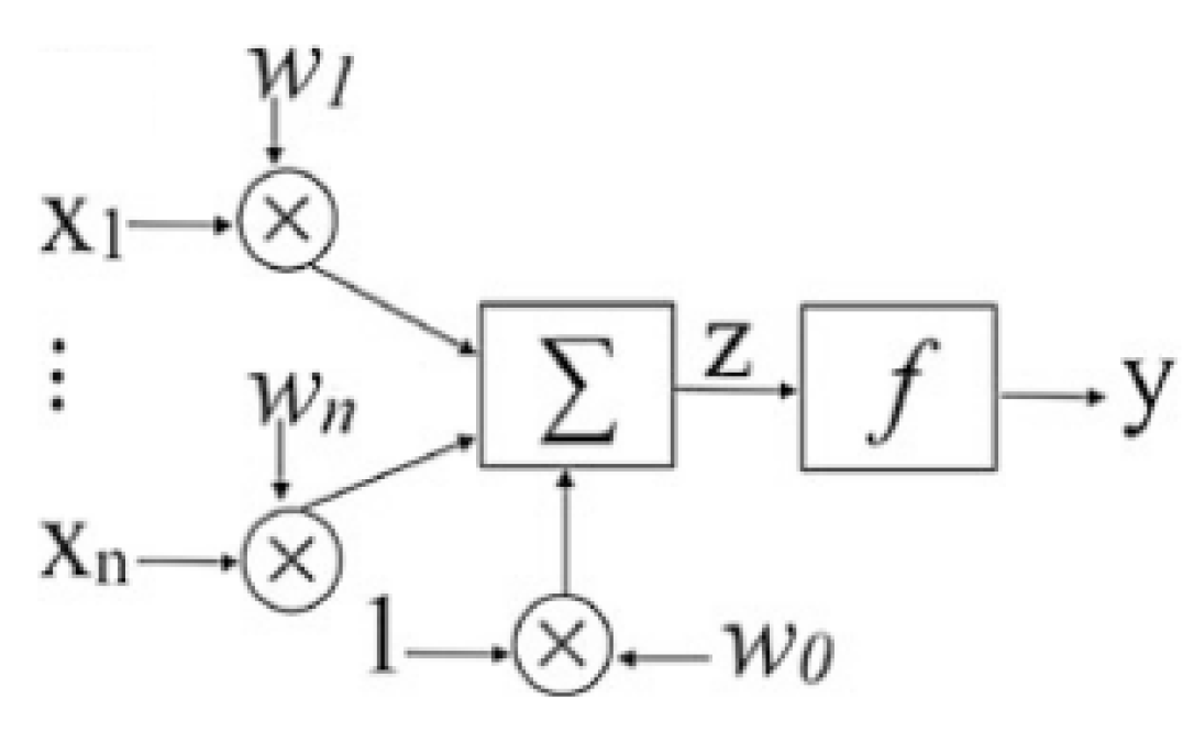
To comprehend the structure and function of the multilayer perceptron (MLP), it is essential first to examine its foundational components: the single-neuron perceptron and the single-layer perceptron. The single-neuron perceptron represents the simplest form of a neural network, consisting of a single output node connected to all input nodes illustrated in
Figure 2. For a perceptron with
n inputs (
), each input
is associated with a corresponding weight
. These inputs represent features or variables, while the output
Y corresponds to a prediction.
The perceptron model operates through three fundamental steps described below:
The activation function determines the output by mapping the weighted sum to a classification or regression, forming the perceptron’s decision-making basis. This process underpins the computational framework of more complex architectures like the MLP.
An extra operation for MLP, compared to RFR, was the scale of features using StandardScaler [
27]. The use of the grid search method showed the best hyperparameters to be employed on it, and they are described as follows:
’solver’: ’sgd’
’momentum’: 0.5
’max_iter’: 500
’learning_rate_init’: 0.1
’learning_rate’: ’invscaling’
’hidden_layer_sizes’: (100,)
’alpha’: 0.01
’activation’: ’tanh’
The hyperparameters are, respectively, constituted by (1) the solver, which specifies the optimization algorithm used to adjust the model’s weights; (2) momentum, a parameter that influences the contribution of previous weight updates to accelerate convergence; (3) max iter, the maximum number of epochs permitted for training; (4) learning rate init, which defines the initial step size for weight adjustments; (5) learning rate, determining the scheme by which the learning rate is updated during training; (6) hidden layer sizes, a specification of the number of neurons in each hidden layer; (7) alpha, a regularization parameter that penalizes large weights to mitigate overfitting; and (8) activation, the function applied at each neuron to introduce non-linearity into the network.
3. Results and Discussion
The field experiments with sugarcane were designed to maximize genetic and agronomic diversity representation across contrasting Brazilian cultivation systems. Four commercially relevant sugarcane cultivars were selected to capture variability in growth cycle characteristics (short-, medium-, and normal phenology) and yield potential. Trials were conducted at two geographically distinct sites to explore the potential of genotype × environment (G×E) interactions: Tambaú (semi-arid climate; average of 550 mm annual rainfall, Udult soil type, moderate fertility) and Piracicaba (temperate humid climate; average of 1,300 mm annual rainfall, Eutrustox soil type, high fertility).
Agronomic management protocols also diverged between experimental fields to reflect regional practices. The Tambaú trial employed conventional stalk planting using locally sourced propagation material from adjacent commercial fields, simulating traditional farming conditions. In contrast, the Piracicaba trial utilized an advanced propagation system involving pre-sprouted seedlings (PSS), which were acclimatized in a controlled nursery environment prior to field transplantation. This dual-site approach enabled comparative analysis of both genetic diversity responses to abiotic stress gradients (water availability, soil fertility) and the impact of propagation technology on crop establishment efficiency.
Figure 3 presents a comprehensive time-series analysis of six vegetation indices (EVI, EVI2, GNDVI, HUE, NDVI, OSAVI) across the sugarcane crop cycle, encompassing both the plant cane and first ratoon phases, for the experimental fields located in Piracicaba (a) and Tambaú (b). Preliminary analysis identified optimal temporal windows (highlighted by shaded regions) corresponding to peak of biomass accumulation during critical growth phases. These intervals align with key phenological stages characterized by rapid physiological development, including maximum leaf canopy expansion, which drives photosynthetic efficiency and biomass production. The selected periods were integrated into predictive models to establish robust correlations between spectral indices and yield outcomes, leveraging the temporal sensitivity of vegetation indices to crop vigor during phases of heightened metabolic activity.
Figure 3 also shows the time series of one of these indices (OSAVI), consolidated across the four varieties, for one of the experimental areas, compared with the time series of an index not selected (SET INDEX).
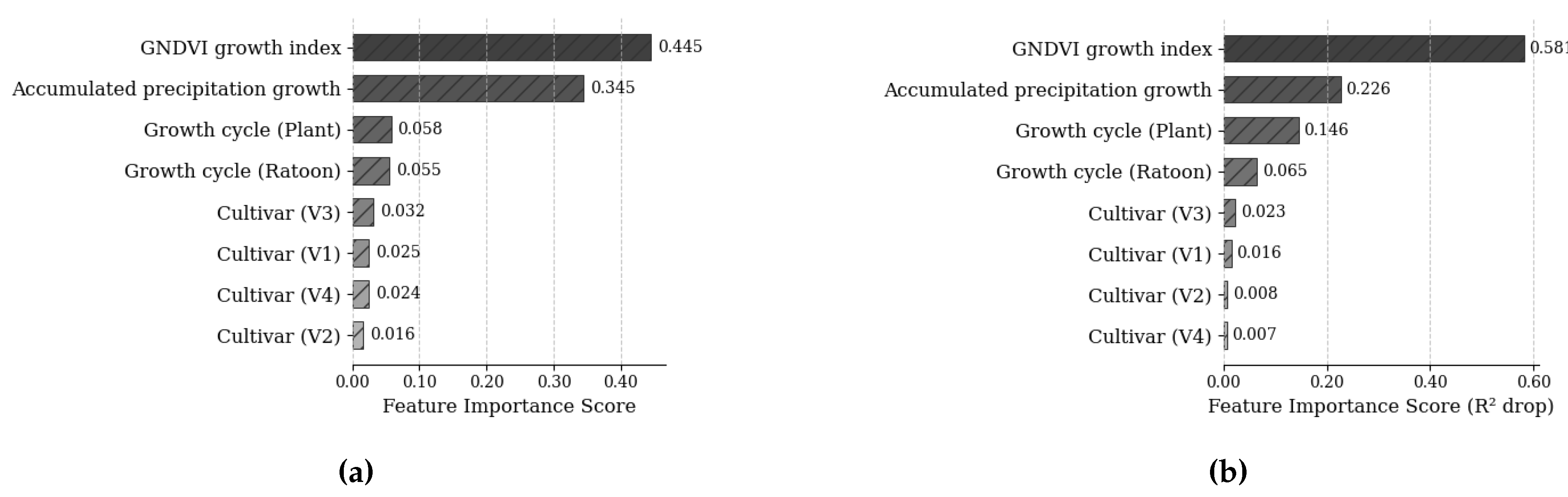
After that, an initial parameter filtering process was carried out to identify key predictors using the normalized relative feature importance scores derived from the Random Forest model’s mean decrease in impurity metric (
Figure 4a,b). Higher scores reflect stronger predictive contributions. Variables retained for modeling exhibited low multicollinearity, with variance inflation factor (VIF) values all below the threshold of 5. These included sugarcane variety, growth cycle, accumulated precipitation (during the growth phase), and mean GNDVI (growth phase).
Subsequently, the heteroskedastic GA regression, Random Forest, and Neural Network models were trained exclusively on these selected variables to mitigate multicollinearity risks, ensuring robust and interpretable model performance.
3.1. Heteroskedastic GA Regression - Training Data from the Experimental Data
3.1.1. Statistical Model
The final heteroskedastic GA regression model selected based on the GAIC has the systematic components given by:
and
3.1.2. Descriptive Statistics
Based on the descriptive analysis of the training data for the response variable tons of sugarcane per hectare (: TCH, t ), different behavior patterns are observed according to the analyzed variables.
For the variable Varieties (: V1, V2, V3, and V4), the average TCH ranged from 111.30 t to 122.21 t . Variety V1 exhibited the lowest mean (111.30 t ), while variety V3 had the highest mean (122.21 t ). Regarding dispersion, the standard deviation was 26.10 for variety V1 and 23.16 for variety V3, suggesting that while variety V3 has the highest mean, it also shows lower variability in production than V1.
In the analysis of
Cycles (
: cane plant and first ratoon), the cane plant cycle recorded an average of 106.93 t
, while the first ratoon cycle achieved a higher average of 127.98 t
. The standard deviation for the plant cycle was 27.60, compared to 22.37 for the first ratoon cycle. These results indicate that the first ratoon cycle has a higher average yield and lower variability, suggesting a more stable production compared to the cane plant cycle.
Table 2.
Estimates of the average yield in tons of sugarcane per hectare (: TCH, t ) and Standard Deviation (SD) based on varieties (), and cycle ().
Table 2.
Estimates of the average yield in tons of sugarcane per hectare (: TCH, t ) and Standard Deviation (SD) based on varieties (), and cycle ().
| |
Category |
Mean |
Standard Deviation |
| Varieties () |
V1 |
111.30 |
26.10 |
| |
V2 |
120.80 |
27.89 |
| |
V3 |
122.21 |
23.16 |
| |
V4 |
115.53 |
30.28 |
| Cycle () |
Cane Plant |
106.93 |
27.60 |
| |
First ratoon |
127.98 |
22.37 |
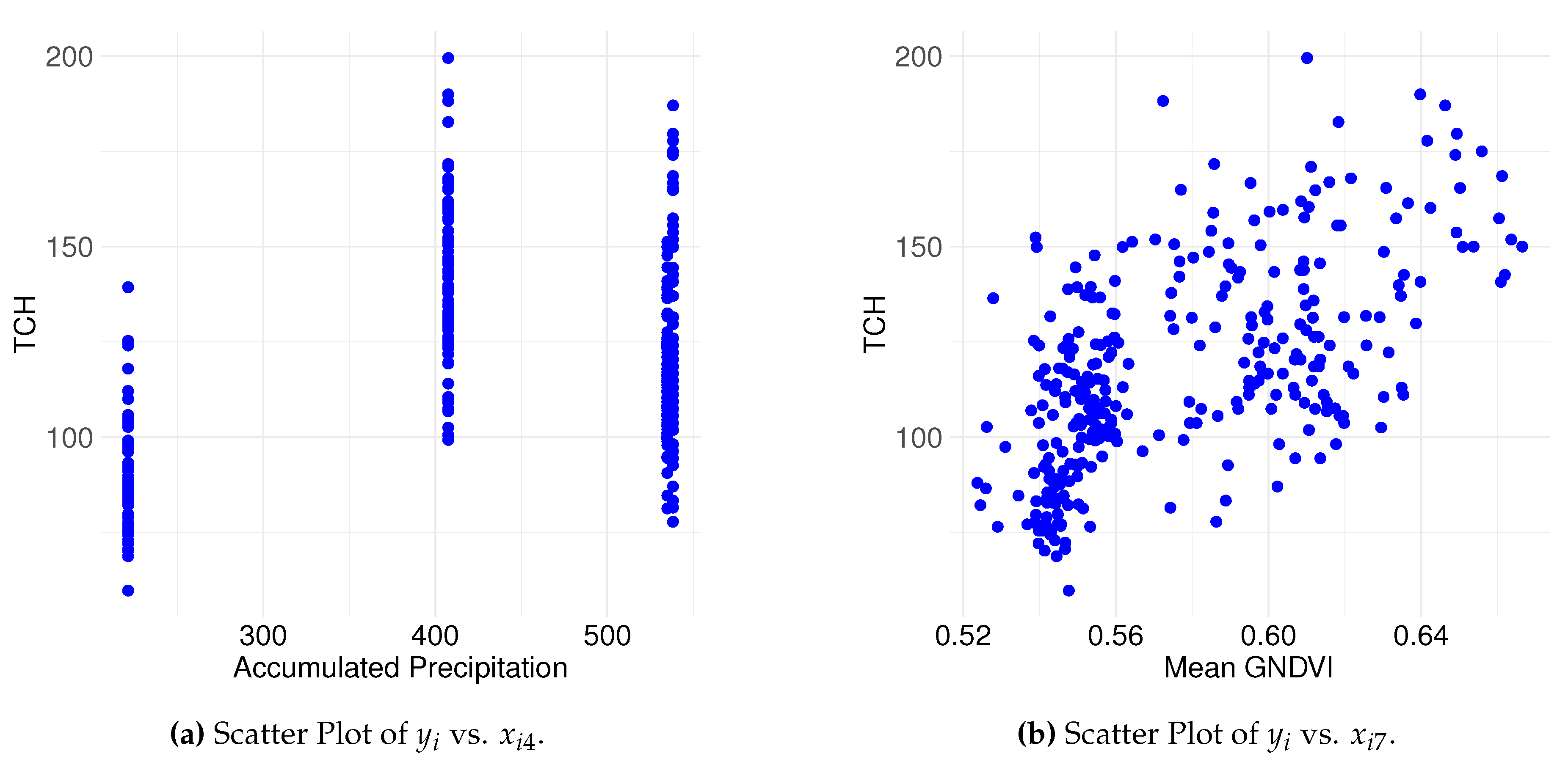
Figure 5 presents scatter plots highlighting the relationships between
(tons of sugarcane per hectare (TCH, t
)) and two explanatory variables (
(Accumulated Precipitation during the growth phase) and
(mean GNDVI during the growth phase)). These variables were selected for graphical representation because they are continuous and allow a direct visualization of their relationships with the response variable.
Figure 5(a) shows the scatter plot of
versus
. The data suggest that precipitation levels influence sugarcane production in non-uniform ways, with no discernible linear relationship observed. Conversely,
Figure 5(b) displays the relationship between TCH and
(mean GNDVI during the growth phase), where the data distribution suggests a potential linear relationship between vegetative growth and sugarcane productivity. This plot provides an initial view of how plant vegetative vigor, measured by mean GNDVI during the growth phase, might be associated with biomass production.
3.1.3. Heteroskedastic GA Regression Results
Table 3 presents the results of the heteroscedastic GA regression model adjusted for the response variable
, representing tons of sugarcane per hectare (TCH, t
). The mean
is modeled using the logarithmic link function according to the specified structure in (
2). Below are the main interpretations of the estimated coefficients and their significance in the context of the response variable.
-
Varieties (, , and ):
- −
The coefficient and p-value = 0.0039 represents the effect of variety relative to the reference variety , and is statistically significant;
- −
The coefficient and p-value = 0.0005 represents the effect of variety relative to the reference variety , and is also statistically significant;
- −
The coefficient and p-value = 0.8000 represents the effect of variety relative to the reference variety , but is not statistically significant;
Cycle (): The coefficient and p-value < 0.0001 is statistically significant and represents the effect of the "Ratoon" level relative to the reference level "Planting".
Mean GNDVI (): The mean GNDVI vegetation index during the growth phase has the highest coefficient, , and a p-value < 0.0001, indicating strong statistical significance. This result suggests that GNDVI is an important variable in sugarcane production, significantly influencing the mean TCH.
For the square root of the dispersion parameter
, which is also modeled using the logarithmic link function as shown in (
2), and indicates variability in TCH production:
Accumulated Precipitation (): The coefficient (p-value = 0.0033) suggests that accumulated precipitation has a statistically significant effect on reducing variability in sugarcane productivity.
Mean GNDVI (): The coefficient and p-value = 0.0095 suggest that GNDVI significantly influences variability in sugarcane yield.
These results underscore the importance of the selected variables in explaining both the mean and variability of sugarcane production. Climatic and agronomic variables have a significant impact on yield, with statistical significance determined by p-values < 0.05, as presented in the table.
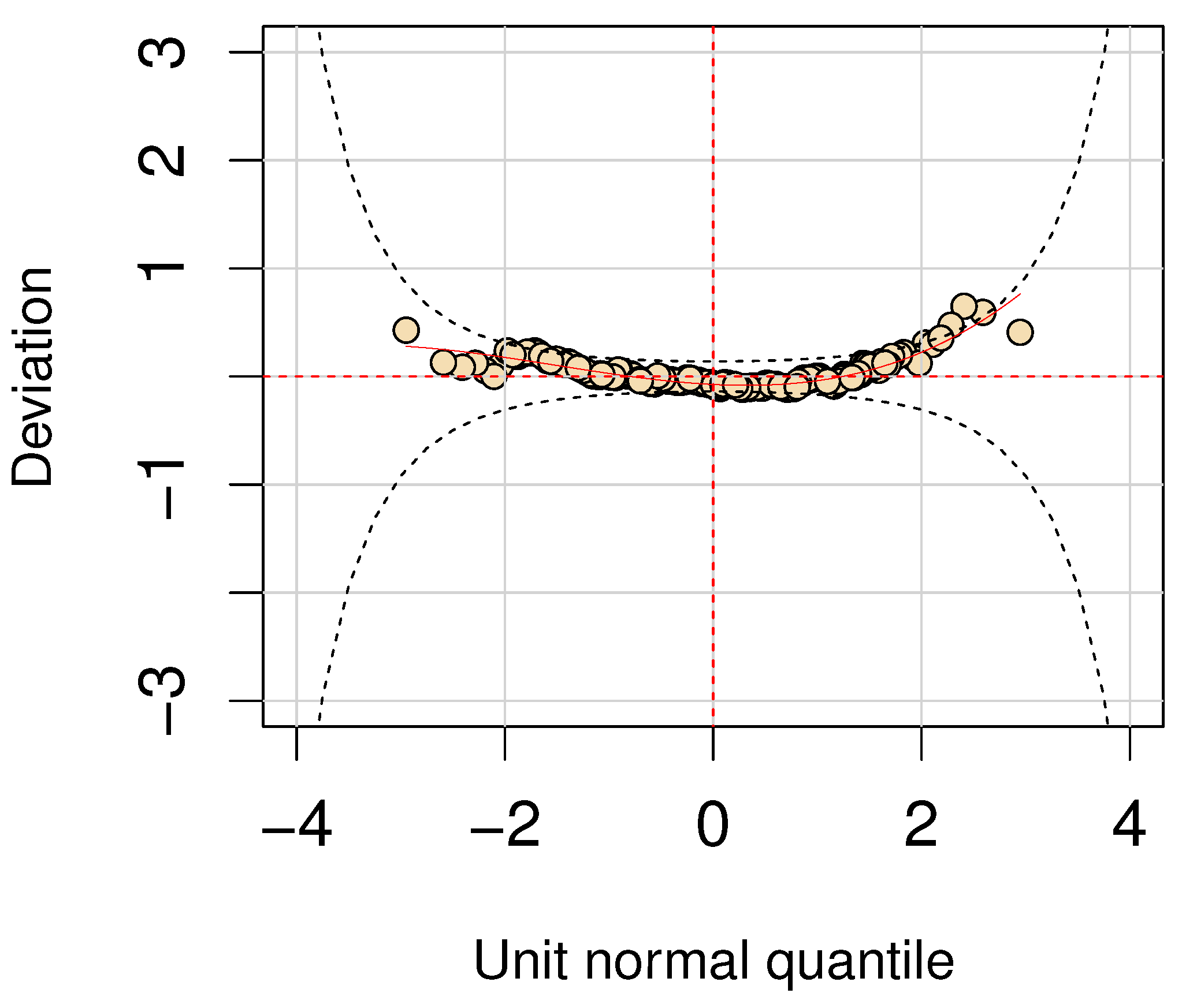
Figure 6 presents the residual analysis of the heteroskedastic GA regression model. The worm plot [
7] indicates that the model fits the data well, suggesting its suitability for analyzing data with similar characteristics in the present study.
3.2. Machine Learning Models Results
The dataset utilized in this study for generalization was insufficient to effectively implement an Artificial Neural Network (ANN) model, as demonstrated by the comparative performance outcomes. The results obtained from the ANN were notably inferior to those achieved using the heteroskedastic GA regression model and the Random Forest (RF) approach. This discrepancy arises from the inherent nature of ANNs, which typically require large volumes of data to accurately extract meaningful features and build robust predictive models [
45]. Given the limited dataset available in this study, the ANN struggled to generalize patterns effectively, leading to suboptimal performance. Consequently, the study highlights the critical importance of dataset size when selecting modeling techniques, particularly for data-intensive methods like ANNs, and underscores the advantages of alternative approaches such as heteroskedastic GA regression and RF in scenarios with constrained data availability.
3.3. Model Performance Analysis for Field Experiment Data
The analysis of the train and test results demonstrates that all three models - Heteroskedastic GA Regression Model, Neural Network, and Random Forest - are suitable for explaining the variability in the dataset.
Table 4 presents the performance metrics for each model, highlighting their ability to provide accurate predictions with comparable levels of error.
All models demonstrate similar levels of predictive performance, with their values showing close results across both training and testing datasets. The Mean Absolute Error (MAE) and Root Mean Squared Error (RMSE) values further indicate that these models provide accurate predictions with comparable error levels. These results highlight the suitability of the Heteroskedastic GA Regression Model, Random Forest and Neural Network for modeling the dataset, offering viable approaches for capturing the dataset’s underlying relationships and variability.
3.4. Performance Evaluation of the Model Using Data from Commercial Sugarcane Fields
This subsection presents the performance of the models - Heteroskedastic GA Regression Model, Neural Network, and Random Forest - when applied to commercial area data for sugarcane productivity (see Table 7 of the supplementary data). These models were evaluated on data not used in the field experiment, providing a measure of their generalization capability. The performance metrics for each model are shown in
Table 5, highlighting the ability of the models to generalize and predict productivity in commercial settings.
The results in
Table 5 show that the models exhibit varying performance when applied to commercial area data. The Heteroskedastic GA Regression Model achieved the highest
of 0.89, indicating a strong ability to explain the variability in sugarcane productivity. This model also had the lowest MAE and RMSE, suggesting it provides accurate and precise predictions for the commercial area data.
In contrast, the Random Forest model showed an of 0.67, indicating a moderate fit, with a notably higher MAE and RMSE values, which suggest less predictive accuracy than the Heteroskedastic GA Regression Model. The Neural Network model performed the weakest among the three, with an of only 0.04, indicating poor performance. Its higher MAE and RMSE values further highlight its limited ability to generalize well to the commercial data from few samples.
These results indicate that, while all models exhibited varying levels of performance depending on the data source, the Heteroskedastic GA Regression Model significantly outperformed the others when applied to commercial area data. In the field experiments, the models performed similarly, with Random Forest showing slightly better results. However, for the commercial area data, the Heteroskedastic GA Regression Model achieved the highest and the lowest MAE and RMSE values, while Random Forest showed moderate performance and the Neural Network model struggled, indicating its limited generalization ability for this particular application. This highlights the importance of selecting the appropriate model based on the nature of the data, as the Heteroskedastic GA Regression Model appears to be more suitable for predicting sugarcane productivity in commercial areas.
4. Conclusions
This study investigated the estimation of sugarcane productivity at harvest through temporal satellite imagery analysis during critical growth phases. The heteroskedastic GA regression model demonstrated superior performance, achieving an of 0.89 and low prediction errors (MAE = 3.9037, RMSE = 5.0870) in commercial sugarcane fields, significantly outperforming both Random Forest and Artificial Neural Network models. Key covariates driving the model’s predictive capability included sugarcane variety (), growth cycle profile (), cumulative precipitation during the growth phase (), and the mean GNDVI spectral index during the growth phase (), which collectively captured agronomic and environmental dynamics during crop development.
The model’s robustness underscores the value of integrating satellite-derived spectral indices (e.g., mean GNDVI during the growth phase) with field-specific agronomic variables, enabling precise monitoring of productivity trends. These findings advocate heteroskedastic GA regression as a scalable tool for agricultural analytics, particularly in data-scarce regions, while emphasizing the necessity of strategic covariate selection to enhance predictive accuracy in crop yield modeling.
Author Contributions
The experiments were designed and carried out in the field by G.M.A.C.; The data were analyzed by J.C.S.V., C.S.A., E.A.S., J.F.G.A., G.M.A.C. and L.A.F.B. The article was written and reviewed by J.C.S.V., C.S.A., E.A.S., J.F.G.A., L.A.F.B., and G.M.A.C. All authors have read and agreed to the published version of the manuscript.
Funding
This work was funded through collaborative grants from the Brazilian Agricultural Research Corporation (Embrapa), the São Paulo State Sugarcane Growers’ Cooperative (Coplacana), and the Foundation for Research and Development Support (Faped) [Grant SEG 30.19.90.005.00.00], as well as Embrapa, the Symbiosis Innovation Program (Simbiose), the Brazilian Funding Authority for Studies and Projects (Finep), and Faped [Grant SEG 20.24.00.110.00.00]. The funders had no role in study design, data collection/analysis, or decision to publish.
Institutional Review Board Statement
Not applicable.
Informed Consent Statement
Not applicable.
Data Availability Statement
To verify the possibility of using the data available in the supplementary material or the images collected in the field, please contact the corresponding author.
Acknowledgments
The authors thank FINEP (Financiadora de Estudos e Projetos) and Simbiose Company for financial support and COPLACANA (Cooperativa de Plantadores de Cana do Estado de São Paulo) for their invaluable support throughout the field experiments.
Abbreviations
The following abbreviations are used in this manuscript:
| ANNs |
Artificial Neural Networks |
| CART |
Classification And Regression Tree |
| EVI |
Enhanced Vegetation Index |
| EVI2 |
Enhanced Vegetation Index 2 |
| GA |
gamma |
| GAIC |
Generalized Akaike Information Criterion |
| GLM |
Generalized Linear Model |
| GNDVI |
Green Normalized Difference Vegetation Index |
| HUE |
Index hue |
| MAE |
Mean Absolute Error |
| MLP |
Multi-Layer Perceptron |
| NDVI |
Normalized Difference Vegetation Index |
| OSAVI |
Optimized Soil Adjusted Vegetation Index |
| pdf |
probability density function |
|
Coefficient of Determination |
| RF |
Random Forest |
| RFR |
Random Forest Regression |
| RMSE |
Root Mean Squared Error |
| SE |
Standard Error |
| TCH |
Tons of cane per hectare |
| VIF |
Variance Inflation Factor |
References
- Acker, J., Williams, R., Chiu, L., Ardanuy, P., Miller, S., Schueler, C., Vachon, P.W. Manore, M. Remote Sensing from Satellites, Reference Module in Earth Systems and Environmental Sciences, PUBLISHER: Elsevier, (2014), ISBN: 978-0-12-409548-9. Available in: https://www.sciencedirect.com/science/article /pii/B9780124095489094409. [CrossRef]
- Amankulova, K., Farmonov, N., Akramova, P., Tursunov, I. & Mucsi, L. Comparison of PlanetScope, Sentinel-2, and landsat 8 data in soybean yield estimation within-field variability with random forest regression. Heliyon. 9 (2023).
- Belsley D.A, Kuh E. and Welsch R.E. (1980) Regression Diagnostics: Identifying Influential Data and Sources of Collinearity, New York: John Wiley & Son.
- Bishop, C. M. Neural networks for pattern recognition, (1995), PUBLISHER: Oxford University Press.
- Breiman, L. (2001). Random forests. Machine Learning, vol. 45, no. 1, pp. 5–32. [CrossRef]
- Breiman, L., Friedman J.H., Olshen, R.A. and Stone, C.J. (1984). Classification And Regression Trees, Routledge Publisher, (1984). [CrossRef]
- Van Buuren, S., Fredriks, M. Worm plot: simple diagnostic device for modelling growth reference curves. Statistics in Medicine, 20, 1259–1277 (2001). [CrossRef]
- Canata, T. F., Wei, M. C. F, Maldaner, L. F., Molin, J. P. Sugarcane Yield Mapping Using High-Resolution Imagery Data and Machine Learning Technique, Remote Sensing, vol. 13, (2021), ISSN: 2072-4292. Available in: https://www.mdpi.com/2072-4292/13/2/232. [CrossRef]
- Cao, J., Zhang, Z.,Tao, F., Zhang, L.,Luo, Y.,Zhang, J.,Han, J.,Xie, J. Integrating Multi-Source Data for Rice Yield Prediction across China using Machine Learning and Deep Learning Approaches, Agricultural and Forest Meteorology, vol. 297, pp. 108275, (2021), ISSN: 0168-1923. Available in: https://www.sciencedirect.com/science/article/pii/S0168192320303774. [CrossRef]
- Escadafal, R. Soil spectral properties and their relationships with environmental parameters-examples from arid regions. Imaging Spectrometry - A Tool For Environmental Observations. pp. 71-87 (1994). [CrossRef]
- Evett, I., Jackson, G., Lambert, J. & McCrossan, S. The impact of the principles of evidence interpretation on the structure and content of statements.. Science & Justice: Journal Of The Forensic Science Society. 40, 233-239 (2000). [CrossRef]
- Food and Agriculture Organization of the United Nations (2023) - with major processing by Our World in Data. "Sugar cane production - FAO [dataset]". Food and Agriculture Organization of the United Nations, “Production: Crops and livestock products” [original data]. Retrieved December 10, 2024 from https://ourworldindata.org/grapher/sugar-cane-production.
- Frazier, A.E.; Hemingway, B.L. A Technical Review of Planet Smallsat Data: Practical Considerations for Processing and Using PlanetScope Imagery. Remote Sens. 2021, 13, 3930. [CrossRef]
- Gitelson, A.A., Kaufman, Y. J., Merzlyak, M. N. Use of a green channel in remote sensing of global vegetation from EOS-MODIS, Remote sensing of Environment, vol. 58, n. 3, pp.289–298, PUBLISHER: Elsevier, (1996).
- ackson, R. D., Huete, A. R. Interpreting vegetation indices, Preventive Veterinary Medicine, vol. 11, num. 3, pp. 185-200, (1991), ISSN: 0167-5877, Available in: https://www.sciencedirect.com/ science/article/pii/S0167587705800042. [CrossRef]
- Jiang, Z., Huete, A., Didan, K. & Miura, T. Development of a two-band enhanced vegetation index without a blue band. Remote Sensing Of Environment. 112, 3833-3845 (2008). [CrossRef]
- Johnson, N. L., Kotz, S., and Balakrishnan, N. (1994). Continuous univariate distributions, volume 1. Wiley, New York, 2nd edition.
- Khanal, S.,Fulton, J., Klopfenstein, A.,Douridas, N., Shearer, S. Integration of high resolution remotely sensed data and machine learning techniques for spatial prediction of soil properties and corn yield Computers and Electronics in Agriculture, vol. 153, pp. 213–225, (2018), ISSN: 0168-1699. Available in: https://www.sciencedirect.com/science/article/pii/S0168169918300334. [CrossRef]
- Kingsford, C. & Salzberg, S. What are decision trees?. Nature Biotechnology. 26, 1011-1013 (2008). [CrossRef]
- Kleidon, A., Fraedrich, K., Heimann, M. (2000). A green planet versus a desert world: Estimating the maximum effect of vegetation on the land surface climate. Climatic Change, 44, 471-493. [CrossRef]
- Krogh, A. What are artificial neural networks?. Nature Biotechnology. 26, 195-197 (2008). [CrossRef]
- McCullagh, P., and Nelder, J. A. (1989). Generalized linear models, Chapman & Hall, London, 2nd edition.
- Molin, J. P., Wei, M. C. F., & da Silva, E. R. O. (2024). Challenges of Digital Solutions in Sugarcane Crop Production: A Review.AgriEngineering, 6(2), 925-946. [CrossRef]
- Monteiro, L. A., Sentelhas, P. C., Pedra, G. U. (2018). Assessment of NASA/POWER satellite-based weather system for Brazilian conditions and its impact on sugarcane yield simulation. International Journal of Climatology, v.38, n.3, pp. 1571-1581. [CrossRef]
- Nelder, J. A., Wedderburn, R. W. (1972). Generalized linear models. Journal of the Royal Statistical Society Series A: Statistics in Society, v. 135, n. 3, pp. 370-384. [CrossRef]
- Oliveira, R., Barbosa Júnior, M., Pinto, A., Oliveira, J., Zerbato, C. & Furlani, C. Predicting sugarcane biometric parameters by UAV multispectral images and machine learning. Agronomy. 12, 1992 (2022). [CrossRef]
- F. Pedregosa, G. Varoquaux, A. Gramfort, V. Michel, B. Thirion, O. Grisel, M. Blondel, P. Prettenhofer, R. Weiss, V. Dubourg, et al. Scikit-learn: Machine learning in python. The Journal of Machine Learning Research, 12:2825–2830, 2011.
- Peel, M. C., McMahon, T. A., Finlayson, B. L., Watson, F. G. (2001). Identification and explanation of continental differences in the variability of annual runoff. Journal of Hydrology, 250(1-4), 224-240. [CrossRef]
- Prataviera, F., Hashimoto, E. M., Ortega, E. M., Savian, T. V., and Cordeiro, G. M. Interval-Censored Regression with Non-Proportional Hazards with Applications. Stats, 6, pp. 643-656 (2023). [CrossRef]
- Quinlan, J. R. (1993). C4.5: programs for machine learning, ISBN: 1-55860-238-0, Morgan Kaufmann Publishers Inc. (1993).
- Ripley, B. et al. (2013). Package ‘mass’. Cran r, v. 538, pp. 113-120.
- Rondeaux, G., Steven, M. & Baret, F. Optimization of soil-adjusted vegetation indices. Remote Sensing Of Environment. 55, 95-107 (1996). [CrossRef]
- Rouse, J. W. Monitoring vegetation systems in the great plains with ERTS, Third ERTS Symposium, NASA, Washington, DC., vol. 1, pp. 309-317, (1973), Available in: https://ci.nii.ac.jp/naid/10016878383/en.
- Sakamoto, T. Incorporating environmental variables into a MODIS-based crop yield estimation method for United States corn and soybeans through the use of a random forest regression algorithm ISPRS Journal of Photogrammetry and Remote Sensing, vol. 160, pp. 208–228, (2020), ISSN: 0924-2716. Available in: https://www.sciencedirect.com/science/article/pii/S0924271619303065. [CrossRef]
- Santos, D.P., Soares, A., de Medeiros, G., Christofoletti, D., Arantes, C.S., Vasconcelos, J.C.S., Speranza, E.A., Barbosa, L.A.F., Antunes, J.F.G., and Cançado, G.M.A. (2024). Evaluation of sugarcane yield response to a phosphate-solubilizing microbial inoculant: Using an aerial imagery-based model. Sugar Tech, v.26, n.1, pp.143–159. [CrossRef]
- Santos Luciano, A., Picoli, M., Duft, D., Rocha, J., Leal, M. & Le Maire, G. Empirical model for forecasting sugarcane yield on a local scale in Brazil using Landsat imagery and random forest algorithm. Computers And Electronics In Agriculture. 184 pp. 106063 (2021). [CrossRef]
- Simoes, M. S., Rocha, J. V., Lamparelli, R. A. M. Spectral variables, growth analysis and yield of sugarcane, Scientia Agricola, vol. 62, (2005), Available in: https://www.scielo.br/j/sa/a/Swxhz5WyRm36YyBTyWNGRPP.
- Song, W., Mu, X., Ruan, G., Gao, Z., Li, L., Yan, G. Estimating fractional vegetation cover and the vegetation index of bare soil and highly dense vegetation with a physically based method, International Journal of Applied Earth Observation and Geoinformation, vol. 58, pp. 168-176, (2017), ISSN: 0303-2434,. Available in: https://www.sciencedirect.com/science/article/pii/S0303243417300144. [CrossRef]
- Stasinopoulos, D.M. and Rigby, R.A. (2008). Generalized additive models for location scale and shape (GAMLSS) in R. Journal of Statistical Software, v.23, pp.1–46.
- Stasinopoulos, M.D., Rigby, R.A., Heller, G.Z., Voudouris, V. and De Bastiani, F. (2017). Flexible regression and smoothing: using gamlss in R. CRC Press, New York.
- Taud, H. & Mas, J. Multilayer perceptron (MLP). Geomatic Approaches For Modeling Land Change Scenarios. pp. 451-455 (2018).
- The Power Data Access Viewer. (2022). Available in: https://power.larc.nasa.gov/data-access-viewer/. Accessed on: October 30.
- Vasconcelos, J. C. S., Ortega, E. M. M., Cordeiro, G. M., Vasconcelos, J. S., and Biaggioni, M. A. M. Estimation and Diagnostic for a Partially Linear Regression based on an Extension of the Rice Distribution. REVSTAT-Statistical Journal, 22, pp. 433-454 (2024).
- Wiegand, v, Richardson, A.J., Escobar, D.E., Gerbermann, A.H. Vegetation indices in crop assessments, Remote Sensing of Environment, volume 35, number 2, pp 105-119, (1991), issn 0034-4257. Available in: https://www.sciencedirect.com/science/article/pii/003442579190004P. [CrossRef]
- Zhang, Y. & Yang, Q. A Survey on Multi-Task Learning. IEEE Transactions On Knowledge And Data Engineering. 34, 5586-5609 (2022).
Figure 2.
Perceptron model, where ... corresponds to the inputs, where ... to the weights, Z is the result of the summarization of the multiplication of the entries by their respective weights made by the neuron and given to the activation function f, and Y corresponds to the output.
Figure 2.
Perceptron model, where ... corresponds to the inputs, where ... to the weights, Z is the result of the summarization of the multiplication of the entries by their respective weights made by the neuron and given to the activation function f, and Y corresponds to the output.
Figure 3.
Time-series analysis of six key vegetation indices (EVI, EVI2, GNDVI, HUE, NDVI, OSAVI) across the two sugarcane production cycles and two locations: (a) Piracicaba, SP, Brazil; and (b) Tambaú, SP, Brazil. The shaded regions highlight periods corresponding to the crop’s peak growth phase, which were incorporated into predictive models to estimate sugarcane productivity.
Figure 4.
(a) Normalized relative feature importance scores from the Random Forest model via mean decrease in impurity. Higher values indicate a greater contribution to the model. (b) Feature importance scores from the MLP model using permutation importance. The importance scores represent the average decrease in the R2 metric when each feature is permuted, indicating the significance of each feature in the model’s predictive performance.
Figure 5.
(a) and (b) show the scatter plots of TCH against cumulative precipitation and the mean GNDVI during the growth phase, respectively.
Figure 5.
(a) and (b) show the scatter plots of TCH against cumulative precipitation and the mean GNDVI during the growth phase, respectively.
Figure 6.
Residual analysis plot evaluating the model’s fit to the data.
Figure 6.
Residual analysis plot evaluating the model’s fit to the data.
Table 3.
Estimates of the parameters, Standard Error (SE), and p-value of the heteroskedastic GA regression model adjusted for the training data. The notation (*) denotes the statistical significance of the variables, indicating p-value < 0.05.
Table 3.
Estimates of the parameters, Standard Error (SE), and p-value of the heteroskedastic GA regression model adjusted for the training data. The notation (*) denotes the statistical significance of the variables, indicating p-value < 0.05.
| Parameter |
Effects |
Parameter |
Estimate |
SE |
Value-p
|
| |
Intercept |
|
2.1760 |
0.1472 |
<0.0001* |
| |
|
|
0.0670 |
0.0232 |
0.0039* |
| |
|
|
0.0846 |
0.0242 |
0.0005* |
|
|
|
0.0060 |
0.0238 |
0.8000 |
| |
|
|
0.2214 |
0.0169 |
<0.0001* |
| |
|
|
4.1985 |
0.2546 |
<0.0001* |
| |
Intercept |
|
-3.5966 |
0.7345 |
<0.0001* |
|
|
|
-0.0008 |
0.0003 |
0.0033* |
| |
|
|
3.4889 |
1.3358 |
0.0095* |
Table 4.
Performance metrics for training and testing data from the Heteroskedastic GA regression model, Random Forest and Neural Network from the experimental field data. Metrics include Coefficient of Determination (), Mean Absolute Error (MAE), and Root Mean Squared Error (RMSE).
Table 4.
Performance metrics for training and testing data from the Heteroskedastic GA regression model, Random Forest and Neural Network from the experimental field data. Metrics include Coefficient of Determination (), Mean Absolute Error (MAE), and Root Mean Squared Error (RMSE).
| Model |
(Train) |
MAE (Train) |
RMSE (Train) |
(Test) |
MAE (Test) |
RMSE (Test) |
| Heteroskedastic GA Regression Model |
0.61 |
13.7743 |
15.6185 |
0.62 |
14.0355 |
14.7355 |
| Random Forest |
0.74 |
10.5100 |
13.9100 |
0.69 |
12.0100 |
16.0500 |
| Neural Network |
0.71 |
11.3200 |
14.7800 |
0.67 |
12.4300 |
16.3900 |
Table 5.
Performance metrics for data of commercial fields from the Heteroskedastic GA regression model, Random Forest, and Neural Network. Metrics include Coefficient of Determination (), Mean Absolute Error (MAE), and Root Mean Squared Error (RMSE).
Table 5.
Performance metrics for data of commercial fields from the Heteroskedastic GA regression model, Random Forest, and Neural Network. Metrics include Coefficient of Determination (), Mean Absolute Error (MAE), and Root Mean Squared Error (RMSE).
| Model |
|
MAE |
RMSE |
| Heteroskedastic GA Regression Model |
0.89 |
3.9037 |
5.0870 |
| Random Forest |
0.67 |
43.4500 |
44.9900 |
| Neural Network |
0.04 |
110.7900 |
112.4900 |
|
Disclaimer/Publisher’s Note: The statements, opinions and data contained in all publications are solely those of the individual author(s) and contributor(s) and not of MDPI and/or the editor(s). MDPI and/or the editor(s) disclaim responsibility for any injury to people or property resulting from any ideas, methods, instructions or products referred to in the content. |
© 2025 by the authors. Licensee MDPI, Basel, Switzerland. This article is an open access article distributed under the terms and conditions of the Creative Commons Attribution (CC BY) license (http://creativecommons.org/licenses/by/4.0/).