Optimal Control of Stochastic Dynamic Systems with Semi-Markov Parameters

The paper considers the generalization of the so-called Markov switching models to the case of generalized semi-Markov switching models, where main model is described by Ito stochastic differential equation. The synthesis problem of the optimal control for a stochastic dynamic system with the semi-Markov parameters is solved. To determine the corresponding functions for Bellman functional and optimal control the system of ordinary differential equations is investigated. The case of linear equations is considered in more detail with closed form of optimal control and corresponding model example.

Keywords:

optimal control

;

stochastic system

;

semi-Markov parameter

Subject:

Computer Science and Mathematics - Mathematics

MSC: 60J25; 93E03; 93E20

1. Introduction

Optimal control synthesis plays a critical role in managing the dynamics of controlled objects or processes. This is particularly relevant when the dynamics are described by Ito stochastic differential equations (SDE). It should be noted that the choice of Ito SDE is due to their prevalence as applied models and their widespread use in biology, chemistry, telecommunications, etc. The main type of random perturbations in stochastic differential equations is the symmetric Wiener process, the trajectories of which have the reflection property, which very well characterizes the symmetry of this process. The symmetry of the solution of the stochastic differential equation is also well reflected in the example of this work, where the symmetry of the solution trajectories is traced relative to the so-called averaged trajectory, and optimal control does not violate this property. The paper [1] considers the optimal control of linear SDE of general type perturbed by a random process with independent increments and a quadratic quality functional. It is shown that under certain conditions the optimal control is linear and can be determined by solving additional vector quadratic problem. The optimal solution of the deterministic problem with feedback is obtained. In paper [2], the theory of optimal control for stochastic systems whose performance is measured by the exponent of an integral form is developed. In paper [3], the problem of the existence of optimal control for stochastic systems with a nonlinear quality functional is solved. Main model in the work [4] is the linear autonomous SDE in the form,

$g (x, u) = A_{0} x + B_{0} u + w_{k} (A_{1} x + B_{1} u),$

(1)

where

$w_{k} \sim i . i . d$ with

$E w_{k} = 0, V a r (w_{k}) = 1$ . It should be noted that the results of the paper are devoted to the quadratic quality functional and necessary and sufficient conditions for the stability of the systems (1), and the stability conditions are formulated in terms of Riccati-type jumping operator properties. Note that the linear case (1) is most often considered as a first approximation of the dynamics of a real phenomenon, since the optimal control in this case can be found in closed form and the approximations of the optimal control can be compared with the exact values.

In the article [5], the main attention is focused on SDE with external switches. In this paper, a number of important remarks are made on the calculation of the product (infinitesimal) operator of a random process given by a SDE with Markov switches.

In the article [6], the main attention is paid to SDE with external switches and Poisson perturbations. Using the Belman equation, sufficient conditions for the existence of optimal control for a general quality function are found, and a closed form of optimal control is found for the linear case with a quadratic quality function.

It should be noted that the transition from difference equations to differential equations gives rise to a number of complications in the synthesis of optimal control, since it leads to a transition from solving more complex dynamical systems such as the analog of the Lyapunov equation for nonautonomous systems. On the other hand, the presence of random variables of different structures leads to the use of the infinitesimal operator [7,8], the calculation of which will depend on the nature of the random variables that affect the calculation of the infinitesimal operator.

In this paper, we will focus on the use of semi-Markov processes [8] as the main source of external random disturbances. It should be noted that the use of semi-Markov processes significantly extends the range of application of theoretical results for many applied problems, since the condition of exponential distribution of the time spent in the state

$θ_{n}$ for continuous Markov processes

$ξ (t), t \geq 0,$ is very strict for many applied problems. A description based on a Markov process will be incorrect if, for example, an assumption is made about the minimum time spent in a particular state

$P (θ_{n} > t_{m i n}) = 1$ , where

$t_{m i n}$ is the minimum time spent in the state. In this case, the use of semi-Markov processes is more efficient, since it allows us to control the properties of the residence time, the size of the jump

${\hat{ξ}}_{n}$ and the interdependence between them based on the semi-Markov kernel

$Q (y, B, t)$ [8]. On the other hand, it should be noted that the use of Markov processes greatly simplifies the study of the system, since it requires estimation only on the basis of the intensities of the Markov process

$λ (y)$ and usually when studying systems with external Markov disturbances it is assumed that

$0 < λ_{m i n} \leq λ (y) \leq λ_{m a x} < \infty, \forall y \in Y .$

In this study, we will not focus on the asymptotic properties of the random process

$x (t), t \geq 0$ , but will consider the problem of synthesizing optimal control on a finite interval

$[0, T]$ , so the article will not consider additional conditions on the semi-Markov process that ensure its ergodicity [7,9,10]. Instead, the main attention will be paid to the elementary study of the dynamics of the main process

$x (t), t \in [0, T],$ at a fixed value of the external perturbation

$ξ (t) = y, y \in Y$ , which allows us to more effectively study the optimal control based on the methods proposed for Markov processes.

In this paper, we consider a model example that illustrates the steps of synthesizing optimal control under the condition that the state residence time is determined by

$θ_{n} = t_{m i n} + P o i s s (λ (y))$ , i.e., the state residence time is discrete and with probability 1 greater than

$t_{m i n}$ .

2. Problem Statement

Consider a stochastic dynamical system defined on a probabilistic basis

$(Ω, F, F, P)$ [7,11]. The system is governed by the stochastic differential equation (SDE):

$d x (t) = a (t, ξ (t), x (t), u (t)) d t + b (t, ξ (t), x (t), u (t)) d w (t), t \in R_{+},$

(2)

with initial conditions

$x (0) = x_{0} \in R^{m}, ξ (0) = y \in Y .$

(3)

Here

$ξ (t), t \geq 0,$ is a semi-Markov process with values in

$Y$ , which characterised by generator [9]

$Q (y, B, t) = P (y, B) F_{y} (t), y \in Y, B \in β_{Y}, t \geq 0,$

(4)

where

$P (y, B)$ specifies the distribution of jumps of the nested Markov chain

${\hat{ξ}}_{n}, n \geq 0$ [8],

$F_{y} (t)$ – is the conditional distribution of time spent in the state y. It should be noted that the representation of the generator based on the splitting (4) greatly simplifies the main calculations in proving the main theoretical results of this paper, but allows generalization to the general case of a semi-Markov kernel

$Q (y, B, t)$ ;

$x : [0, + \infty) \times Ω \to R^{m}$ ;

$w (t), t \geq 0,$ is a standard Wiener process; a control

$u (t) : = u (t, x (t)) : [0, T] \times R^{m} \to R^{m}$ is m-measured function from the set of admissible controls U[12]; the processes w and

$ξ$ are independent [7,11].

As in works [11,13], we assume that the measured by the set of variables functions

$a : R_{+} \times Y \times R^{m} \times U \to R^{m}$ and

$b : R_{+} \times Y \times R^{m} \times U \to R^{m}$ satisfy the boundedness condition and the Lipschitz condition

${| a (t, y, x, u) |}^{2} + {| b (t, y, x, u) |}^{2} \leq {C (1 + | x |}^{2}),$

(5)

$| a (t, y, x_{1}, u) - a (t, y, x_{2}, u) |^{2} + | b (t, y, x_{1}, u) - b (t, y, x_{2}, u) |^{2} \leq L {| x_{1} - x_{2} |}^{2}, x_{1}, x_{2} \in R^{m} .$

(6)

The semi-Markov process

$ξ$ has the following effect on the trajectories of the process x. Suppose that on the interval

$[t_{0} = 0, t_{1})$ the process

$ξ$ takes the value

$y_{1}$ . Then the movement will occur due to the system

$d x (t) = a (t, y_{1}, x (t), u (t)) d t + b (t, y_{1}, x (t), u (t)) d w (t), t \in R_{+}, x (0) = x_{0} \in R^{m} .$

(7)

According to [10,11], if the conditions (5) and (6) are met, the system (7) has on the interval

$[0, t_{1})$ a unique solution with finite second moment up to stochastic equivalence.

Then, at time

$t_{1}$ , the value of the process

$ξ$ changes:

$y_{1} \to y_{2}$ . Then, on the interval

$[t_{1}, t_{2})$ , the motion will occur due to the system

$d x (t) = a (t, y_{2}, x (t), u (t)) d t + b (t, y_{2}, x (t), u (t)) d w (t), t \in R_{+}, x (t_{1}) = x (t_{1} -) \in R^{m} .$

(8)

According to [10,11], if conditions (5), (6) are met, system (8) has a unique solution with a finite second moment on the interval

$[t_{1}, t_{2})$ .

Thus, conditions (5), (6) guarantee the existence of a unique solution to the Cauchy problem (2), (3) on the interval

$[0, + \infty) = ⋃_{k = 0}^{\infty} [t_{k}, t_{k + 1}), 0 = t_{0}, t_{1}, . . ., t_{k}, . . .$ , the second moment for which is finite. Thus, for the existence of a solution on

$[0, \infty)$ , we will assume that the semi-Markov process is defined on

$[0, \infty)$ , i.e.

$\forall T > 0 : P (ξ (T) e x i s t) = 1$ .

3. Sufficient Conditions for Optimality

We introduce a sequence of functions

$v_{k} (t, x) : [t_{k}, T] \times R^{m} \to R^{1}, k \geq 0,$ and class

$V : = {v_{k} (t, x) \in C^{1, 2} (R_{+} \times R^{m})}$ .

On the functions

$v_{k} (t, x) \in V$ we define the weak infinitesimal operator (WIO)

$L v_{k} (t, x) = lim_{Δ \to 0 +} \frac{1}{Δ} {E v_{k} (t + Δ, x (t + Δ, t_{k}, y, u)) - v_{k} (t, x)},$

(9)

where

$x (t) = x (t, t_{k}, y, u)$ is the strong solution (2) on the interval

$t \in [t_{k}, t_{k + 1})$ with control

$u = u_{k} \in U$ .

The problem of optimal control is to find a control

$u_{k}^{0}, k \geq 0,$ from the set U that minimizes the scalar quality functional [12]

$I (u_{k}^{0}) = I^{u_{k}^{0}} (t, x) = inf_{u \in U} (\sum_{k = 0}^{N} E_{t_{k}, x_{k}} \{F (x (T)) + \int_{t}^{T} G (s, x (s), u (s)) d s\}),$

(10)

for some fixed

$T > 0$ ,

$F (x) \geq 0, G (t, x, u) \geq 0$ ,

$E_{t, x} {f} = E {f / x (t) = x}$ , and

$N = m a x {k : t_{k} < T}$ .

To obtain sufficient conditions for optimality, we need to prove several auxiliary statements.

Lemma 1. Let:

1) there exists a unique solution to the Cauchy problem (2), (3), whose second moment is finite for each t;

2) a sequence of functions

$v_{k} : [0, T] \times R^{m} \to R^{1}, k \geq 0,$ from class V exists;

3) for

$s \in [t_{k}, T)$ , the WIO

$L v_{k} (s, x)$ is defined on the solutions of (2), (3).

Then

$\forall {\tilde{t}}_{1}, {\tilde{t}}_{2} \in [t_{0}, T]$ the equality

$E_{t_{k}, x_{k}} v_{k} ({\tilde{t}}_{2}, x ({\tilde{t}}_{2})) - E_{t_{k}, x_{k}} v_{k} ({\tilde{t}}_{1}, x ({\tilde{t}}_{1})) = \int_{{\tilde{t}}_{1}}^{{\tilde{t}}_{2}} E_{t_{k}, x_{k}} L v_{k} (s, x (s)) d s .$

(11)

met.

Proof.

For the Markov process

$x (t, t_{k}, y, u)$ with respect to the

$σ$ -algebra

$F_{{\tilde{t}}_{1}, {\tilde{t}}_{2}}$ constructed on the interval

$[{\tilde{t}}_{1}, {\tilde{t}}_{2}], {\tilde{t}}_{1}, {\tilde{t}}_{2} \in [t_{k}, T]$ , the following Dynkin formula [7] holds

$E_{t_{k}, x_{k}} v_{k} ({\tilde{t}}_{1} + τ ({\tilde{t}}_{2}), x ({\tilde{t}}_{1} + τ ({\tilde{t}}_{2}), t_{k}, y, u))$

$= v_{k} (t, x) + E_{t_{k}, x_{k}} \int_{t_{0}}^{τ_{r} ({\tilde{t}}_{2})} L v_{k} ({\tilde{t}}_{1} + τ, x ({\tilde{t}}_{1} + τ, t_{k}, y, u)) d τ,$

where

$τ_{r} = inf_{t} {| x (t) | > r}$ and

$τ_{r} ({\tilde{t}}_{2}) = min {τ_{r}, {\tilde{t}}_{2}}$ .

$lim_{r \to \infty} τ_{r} ({\tilde{t}}_{2}) = {\tilde{t}}_{2}$ then for the solution of the problem (2), (3) we get the following equality

$E_{t_{k}, x_{k}} v_{k} ({\tilde{t}}_{1} + {\tilde{t}}_{2}, x ({\tilde{t}}_{1} + {\tilde{t}}_{2}, t_{k}, y, u)) = v_{k} (t, x) + E_{t_{k}, x_{k}} \int_{t_{0}}^{{\tilde{t}}_{2}} L v_{k} ({\tilde{t}}_{1} + τ, x ({\tilde{t}}_{1} + τ, t_{k}, y, u)) d τ .$

(12)

Similarly, write the Dynkin formula on the interval

$[t_{0}, t_{1}]$ and, subtracting it from (12), we obtain (11). Lemma 1 is proved. □

Lemma 2. Let:

1) conditions 1) and 2) of Lemma 1 are fulfilled;

2) for

$\forall t \in [t_{0}, T]$ ,

$\forall v_{k} \in V, k \geq 0$ has the sense the equation

$L v_{k} (t, x) + G (t, x, u_{k} (t, x)) = 0,$

(13)

with a boundary condition

$v_{k} (T, x) = 0, k \geq 0,$

(14)

where

$L v_{k} (t, x)$ is the WIO defined by (9).

Then

$v_{k} \in V, k \geq 0$ , can be write as

$v_{k} (t, x) = E_{t_{k}, x_{k}} \{\int_{t}^{T} G (s, x, u (s, x)) d s\}, t \in [t_{k}, T] .$

(15)

Proof.

Consider the solution

$x (t) \in R^{m}$ of the problem (2), (3) for

$t \in [t_{k}, T]$ , constructed according to the corresponding initial condition.

We integrate (13) respect to s from

$t_{k}$ to T and calculate the mathematical expectation. We get

$E_{t_{k}, x_{k}} \{\int_{t_{k}}^{T} L v_{k} (s, x) d s\} + E_{t_{k}, x_{k}} \{\int_{t_{k}}^{T} G (s, x, u_{k} (s, x)) d s\} = 0 .$

(16)

According to Lemma 1, there exists a first term (16) that is equal to the increment (11):

$E_{t_{k}, x_{k}} \{\int_{t_{k}}^{T} L v_{k} (s, x) d s\} = E_{t_{k}, x_{k}} v_{k} (T, x (T)) - E_{t_{k}, x_{k}} v_{k} (t, x) = - v_{k} (t, x),$

where

$E_{t_{k}, x_{k}} v_{k} (T, x (T)) = v_{k} (T, x (T)) = 0$ according to (14), and

$E_{t_{k}, x_{k}} v_{k} (t, x (t)) = v_{k} (t, x)$ . Thus,

$E_{t_{k}, x_{k}} \{\int_{t_{k}}^{T} L v_{k} (s, x) d s\} = - v_{k} (t, x) .$

(17)

Substituting (17) into (16), we obtain the statement of Lemma 2. □

Theorem 1.

Let:

1) there exists a unique solution to the Cauchy problem (2), (3), whose second moment is finite for each t;

2) there exists a sequence of functions

$v_{k} \in V, k \geq 0,$ and an optimal control

$u_{k}^{0} \in U, k \geq 0,$ that satisfy the equation

$L v_{k} (t, x) + G (t, x, u_{k}^{0} (t, x)) = 0,$

(18)

with a boundary condition

$v_{k} (T, x) = F (x (T));$

(19)

$\forall t \in [0, T]$ ,

$\forall u_{k} \in U, k \geq 0,$ the following inequality holds

$L v_{k} (t, x) + G (t, x, u_{k} (t)) \geq 0,$

(20)

where

$L = L (t, x, u)$ is the WIO (9) on the solutions of (2), (3).

Then the control

$u_{k}^{0}$ is optimal and

$\forall t \in [t_{0}, T],$

$I^{u_{k}^{0}} (t, x) = inf_{u \in U} I^{u} (t, x) = v_{k} (t, x) .$

(21)

The sequence of functions

$v_{k} (t, x)$ is called the control cost or Bellman function, and equation (18) can be written as the Bellman equation

$inf_{u \in U} [L (t, x_{k}, u) v_{k} (t, x_{k}) + G (t, x_{k}, u)] = 0 .$

(22)

Proof.

An optimal control is also an admissible control. Therefore, there exists a solution

$x (t_{k}, t_{0}, y, u_{k}^{0})$ for which (18) takes the form

$L v_{k} (t, x (t, t_{k}, y, u_{k}^{0})) + G (t, x (t, t_{k}, y, u_{k}^{0}), u_{k}^{0} (t, x)) = 0,$

(23)

where

$u_{k}^{0}$ taken at the point

$(t, x (t, t_{k}, y, u_{k}^{0})), t \in [t_{k}, t_{k + 1})$ .

We integrate (23) from t to T, calculate the mathematical expectation, and, taking into account (19), we obtain

$v_{k} (t, x) = E_{t_{k}, x_{k}} \{F (x (T)) + \int_{t}^{T} L v_{k} (τ, x (τ, t_{0}, y, u_{k}^{0})) d τ\} .$

Now let

$u_{k} = u_{k} (t)$ be an arbitrary control from the class of admissible controls U. Then, according to condition 3) of the theorem, the following inequality holds

$\forall u_{k} \in U, k \geq 0,$

$L v_{k} (τ, x (τ, t_{0}, y, u_{k})) + G (τ, x (τ, t_{0}, y, u_{k}), u_{k} (τ)) \geq 0,$

(24)

We integrate (24) over

$τ \in [t_{0}, T]$ , and calculate the mathematical expectation

$E$ at fixed

$τ$ and initial value x. Accounting Lemmas 1 and 2, we obtain

$v_{k} (t, x (t, t_{0}, y, u_{k}^{0}))$

$\leq E_{t_{k}, x_{k}} \{F (x (T, u_{k})) + \int_{t_{k}}^{T} G (τ, x (τ, t_{0}, y, u_{k}), u_{k} (τ)) d τ\} = v_{k} (t, x (t, t_{0}, y, u_{k})) .$

And this, in fact, is the definition of optimal control

$u_{k}^{0} (t, x)$ in the sense of minimizing the quality functional

$I^{u} (t, x)$ . Theorem 1 is proved. □

4. General Solution of the Optimal Control Problem

The following theorem holds.

Theorem 2.

The weak infinitesimal operator on the solutions of the Cauchy problem (2), (3) on the functions

$v_{k} (t, x) \in V$ is calculated by the formula

$L v_{k} (t, x) = \frac{\partial v_{k} (t, x)}{\partial t} + (\nabla v_{k} (t, x), a (t, y, x, u))$

$+ \frac{1}{2} S p (b^{T} (t, y, x, u) \cdot \nabla^{2} v_{k} (t, x) \cdot b (t, y, x, u))$

$+ \sum_{i \neq j}^{N} [\int_{R^{m}} v_{k} (t, z; j) p_{i j} (t, z | x) d z - v_{k} (t, x; i)] q_{i j},$

(25)

where

$(\cdot, \cdot)$ is a scalar product,

$(\nabla v_{k}) : = {((\partial v_{k} / \partial x_{1}), . . ., (\partial v_{k} / \partial x_{m}))}^{T}$ ,

$(\nabla^{2} v_{k}) : = {[\partial^{2} v_{k} / \partial x_{i} \partial x_{j}]}_{i, j = 1}^{m}, k \geq 0$ ,

${< <}^{T}$ >> is a transpose sign,

$S p$ is a matrix trace,

$q_{i j} = \lim_{t ↓ 0} \frac{Q (i, j, t)}{t} = P (i, j) F_{x}^{'} (0),$

$p_{i j} (t, z | x)$ is a conditional density of the process

$x (t)$ for

$ξ (t -) = i, ξ (t) = j$ :

$P \{x (t) \in [z, z + d z] | x (t) = x, ξ (t -) = i, ξ (t) = j\} = p_{i j} (t, z | x) d z + o (d z) .$

(26)

In the last term in the formula (25) in the function

$v_{k} (t, x; i)$ the last argument indicates the value of the semi-Markov process at a given time, i.e.

$ξ (t) = y_{i}$ .

Proof.

The first three terms can be obtained in the same way as in [14]. Let us obtain the form of the last term, which is related to the semi-Markov parameter

$ξ$ . To do this, consider the hypotheses

$H_{i j} = {ξ (t -) = i, ξ (t) = j}, i, j \in Y$ . Considering the hypotheses

$H_{i j}$ , we obtain that the last term will correspond to the hypotheses

$H_{i j}, i \neq j$ , i.e.

$E v_{k} (t + Δ, x (t + Δ, t_{k}, y, u)) = \sum_{i, j \in Y} E (v_{k} (t + Δ, x (t + Δ, t_{k}, y, u)) I_{H_{i j}})$

$= \sum_{i = j \in Y} E (v_{k} (t + Δ, x (t + Δ, t_{k}, y, u)) I_{H_{i j}}) + \sum_{i \neq j \in Y} E (v_{k} (t + Δ, x (t + Δ, t_{k}, y, u)) I_{H_{i j}}) .$

For the first term, the absence of a change in the state of the semi-Markov process, the conditions imposed on the coefficients of the initial equation allow us to write

$\lim_{Δ \to 0} \frac{1}{Δ} (\sum_{i = j \in Y} E (v_{k} (t + Δ, x (t + Δ, t_{k}, y, u)) I_{H_{i j}}) - v_{k} (t, x))$

$= \frac{\partial v_{k} (t, x)}{\partial t} + (\nabla v_{k} (t, x), a (t, y, x, u)) + \frac{1}{2} S p (b^{T} (t, y, x, u) \cdot \nabla^{2} v_{k} (t, x) \cdot b (t, y, x, u)) .$

On the other hand, when the state of the semi-Markov process

$ξ (t)$ changes at time t, taking into account the form of the conditional transition probability

$P \{x (t) \in [z, z + d z] | x (t) = x, ξ (t -) = i, ξ (t) = j\}$ (26), we obtain

$\lim_{Δ \to 0} \frac{1}{Δ} (\sum_{i \neq j \in Y} E (v_{k} (t + Δ, x (t + Δ, t_{k}, y, u)) I_{H_{i j}}) - v_{k} (t, x))$

$= \sum_{i \neq j}^{N} [\int_{R^{m}} v_{k} (t, z; j) p_{i j} (t, z | x) d z - v_{k} (t, x; i)] q_{i j} .$

Theorem 2 is proved. □

The first equation for finding

$v_{k}^{0} (t, x), k \geq 0,$ can be obtained by substituting (25) into (18). We get

$\frac{\partial v_{k}^{0} (t, x; i)}{\partial t} + {(\frac{\partial v_{k}^{0} (t, x; i)}{\partial x})}^{T} \cdot a (t, y_{i}, x, u)$

$+ \frac{1}{2} S p (b^{T} (t, y_{i}, x, u) \cdot \frac{\partial^{2} v_{k}^{0} (t, x; i)}{\partial x^{2}} \cdot b (t, y_{i}, x, u))$

$+ \sum_{i \neq j}^{N} [\int_{R^{m}} v_{k}^{0} (t, x; j) p_{i j} (t, z | x) d z - v_{k}^{0} (t, x; i)] q_{i j} + G (t, x, u) = 0$

(27)

with a boundary condition

$v_{k}^{0} (T, x) = F (x) .$

(28)

The second equation, for finding the optimal control

$u_{k}^{0} (t, x)$ , can be obtained from (27) by differentiating respect to u, since

$u = u_{k}^{0}, k \geq 0,$ delivers the minimum of the left-hand side of (27):

$[{(\frac{\partial v_{k}^{0} (t, x; i)}{\partial x})}^{T} \cdot \frac{\partial a (t, y_{i}, x, u)}{\partial u}$

$+ \frac{1}{2} S p [{(\frac{\partial b (t, y_{i}, x, u)}{\partial u})}^{T} \cdot \frac{\partial^{2} v_{k}^{0} (t, x; i)}{\partial x^{2}} \cdot b (t, y_{i}, x, u)$

$+ b^{T} (t, y_{i}, x, u) \cdot \frac{\partial^{2} v_{k}^{0} (t, x; i)}{\partial x^{2}} \cdot \frac{\partial b (t, y_{i}, x, u)}{\partial u}]$

$+ \frac{\partial G (t, x, u)}{\partial u}] |_{u = u_{k}^{0}} = 0,$

(29)

where

$(\partial a / \partial u)$ is a

$m \times m$ -Jacobian, which consists of the elements

${(\partial a_{n} / \partial u_{s}), n = \bar{1, m}, s = \bar{1, m}}$ (

$(\partial b / \partial u)$ – similarly),

$(\partial G / \partial u) \equiv ((\partial G / \partial u_{1}), . . ., (\partial G / \partial u_{r}))$ ,

$k \geq 0$ .

The solution of the system (27), (29) is a very difficult task even with the use of modern computer technologies. Therefore, it is advisable to consider a simplified version of the problem (2), (3), (10), namely, a linear system with a quadratic quality functional.

5. Synthesis of Optimal Control for a Linear Stochastic System

Consider the problem of optimal control for a linear stochastic dynamical system given by the stochastic differential equation

$d x (t) = [A (t, ξ (t)) x (t) + B (t, ξ (t)) u (t)] d t + σ (t, ξ (t)) x (t) d w (t), t \in R_{+},$

(30)

with the initial conditions

$x (0) = x_{0} \in R^{m}, ξ (0) = y \in Y .$

(31)

Here

$A, B, σ$ are piecewise continuous integral matrix-functions of appropriate dimension.

The problem of optimal control for the system (30), (31) is to find a control

$u_{k}^{0}, k \geq 0,$ from the set of admissible controls U such that minimizes the quadratic quality functional

$I (u_{k}) = I^{u_{k}} (t, x) = \sum_{k = 0}^{\bar{N}} E_{t_{k}, x_{k}} \{x^{T} (T) M_{0} (ξ (t)) x (T)$

$+ \int_{t}^{T} [u^{T} (s) M_{1} (s, ξ (s)) u (s) + x^{T} (s) M_{2} (s, ξ (s)) x (s)] d s\},$

(32)

$M_{1} (t, ξ (t))$ is a uniformly positive definite respect to

$t \in [0, T]$

$m \times m$ -matrix,

$M_{0} (ξ (t))$ and

$M_{2} (t, ξ (t))$ are non-negatively definite

$m \times m$ -matrices. To simplify the notation, we introduce the notation

$A_{i} (t) = A (t, y_{i}), B_{i} (t) = B (t, y_{i}), σ_{i} (t) = σ (t, y_{i}),$

$M_{0 i} = M_{0} (y_{i}), M_{1 i} (t) = M_{1} (t, y_{i}), M_{2 i} (t) = M_{2} (t, y_{i}) .$

Theorem 3.

The optimal control for the problem (30)–(32) has the next form:

$u_{k}^{0} (t, x; i) = - M_{1 i}^{- 1} (t) B_{i}^{T} (t) P_{i} (t) x (t),$

(33)

where the non-negatively definite

$m \times m$ -matrix

$P_{i} (t) = P (t, ξ (t))$ defines the Bellman functional

$v_{k}^{0} (t, x; i) = x^{T} (t) P_{i} (t) x (t) + g (t), v_{k}^{0} (T, x; i) = x^{T} (t_{k}) M_{0 i} x (t_{k}) .$

(34)

Here g is a non-negative scalar function.

Proof.

Bellman’s equation for (30)–(32) has the form

$inf_{u \in U} [L v_{k}^{0} (t, x; i) + u_{k}^{T} (t, x; i) M_{1 i} (t) u_{k} (t, x; i) + x^{T} (t) M_{2 i} (t) x (t))] = 0,$

(35)

where

$L v_{k}^{0} (t, x; i) = \frac{\partial v_{k}^{0} (t, x; i)}{\partial t} + \dot{g} (t) + {[A_{i} (t) x (t) + B_{i} (t) u_{k} (t, x; i)]}^{T} \nabla v_{k}^{0} (t, x; i)$

$+ \frac{1}{2} S p (σ_{i}^{T} (t) \cdot \nabla^{2} v_{i}^{0} (t, x; i) \cdot σ_{i} (t))$

$+ \sum_{i \neq j}^{N} [v_{k}^{0} (t, x; j) - v_{k}^{0} (t, x; i)] q_{i j} .$

(36)

Substitute (36) into (35):

$\frac{\partial v_{k}^{0} (t, x; i)}{\partial t} + \dot{g} (t) + {[A_{i} (t) x (t) + B_{i} (t) u_{k} (t, x; i)]}^{T} \nabla v_{k}^{0} (t, x; i)$

$+ \frac{1}{2} S p (σ_{i}^{T} (t) \cdot \nabla^{2} v_{k}^{0} (t, x; i) \cdot σ_{i} (t))$

$+ \sum_{i \neq j}^{N} [v_{k}^{0} (t, x; j) - v_{k}^{0} (t, x; i)] q_{i j} + u_{k}^{T} (t, x; i) M_{1 i} (t) u_{k} (t, x; i) + x^{T} (t) M_{2 i} (t) x (t)) = 0 .$

(37)

The form of the optimal control is obtained by differentiating (37) since

$u_{k} (t, x; i) = u_{k}^{0} (t, x; i)$ minimizes the left side (37):

$u_{k}^{0} (t, x; i) = - \frac{1}{2} M_{1 i}^{- 1} (t) B_{i}^{T} (t) \nabla v_{k}^{0} (t, x; i),$

where

$\nabla v_{k}^{0} (t, x; i) = 2 P_{i} (t) x (t) .$

Therefore,

$u_{k}^{0} (t, x; i) = - M_{1 i}^{- 1} (t) B_{i}^{T} (t) P_{i} (t) x (t) .$

Theorem 3 is proved. □

6. Construction of the Bellman Equation

Substituting (33) and (34) into equation (35), we obtain the following equation for

$\forall t \in [t_{k}, t_{k + 1})$ :

$x^{T} (t) \frac{d P_{i} (t)}{d t} x (t) + \dot{g} (t)$

$+ 2 [A_{i} (t) x (t) - B_{i} (t) M_{1 i}^{- 1} (t) B_{i}^{T} (t) x (t)] P_{i} (t) x (t) + S p (σ_{i}^{T} (t) P_{i} (t) σ_{i} (t))$

$+ \sum_{i \neq j}^{N} [x^{T} (t) P_{j} (t) x (t) - x^{T} (t) P_{i} (t) x (t)] q_{i j}$

$+ {[M_{1 i}^{- 1} (t) B_{i}^{T} (t) P_{i} (t) x (t)]}^{T} M_{1 i} (t) M_{1 i}^{- 1} (t) B_{i}^{T} (t) P_{i} (t) x (t) + x^{T} (t) M_{2 i} (t) x (t) = 0 .$

(38)

Equating to zero the quadratic form in x and expressions that do not depend on x, taking into account the matrix equality

$2 x^{T} P_{i} x = x^{T} (P_{i} A_{i} + A_{i}^{T} P_{i}) x$ , we obtain a system of differential equations for finding the matrices

$P_{i} (t), t \in [t_{k}, t_{k + 1}), k \geq 0$ :

$\frac{d P_{i} (t)}{d t} + A_{i}^{T} (t) P_{i} (t) + P_{i} (t) A_{i} (t) - B_{i} (t) M_{1 i}^{- 1} (t) B_{i}^{T} (t) P_{i} (t) + \sum_{i \neq j}^{N} [P_{j} (t) - P_{i} (t)] q_{i j}$

$+ {[M_{1 i}^{- 1} (t) B_{i}^{T} (t) P_{i} (t)]}^{T} B_{i}^{T} (t) P_{i} (t) + M_{2 i} (t) = 0,$

(39)

$S p (σ_{i}^{T} (t) P_{i} (t) σ_{i} (t)) + \dot{g} (t) = 0,$

(40)

with a boundary condition

$P_{i} (T) = M_{0 i} .$

(41)

Thus, we can formulate the following theorem.

Theorem 4.

If the quality functional for the system (30), (31) is (32), and the control cost is (34), then the system of differential equations for finding the matrices

$P_{i} (t), t \in [t_{k}, t_{k + 1}), k \geq 0,$ has the form (39)–(41).

Next, we will prove the solvability of the system (39)–(41). Let us use the Bellman iteration method [15]. To simplify the calculations, we consider the interval

$[t_{k}, t_{k + 1})$ where

$ξ (t) = y_{i})$ and omit the index k for

$v, u$ and P. Let us define the zero approximation

$u_{0} (t, x) = - M_{1}^{- 1} (t) B^{T} (t) P_{0} (t) x (t),$

(42)

where

$P_{0} (t) \geq 0$ is a bounded piecewise continuous matrix. Substitute (42) into (27) and find the value of

$v_{1} (t, x)$ from the resulting equation, which corresponds to the control of (42).

Next, we substitute

$v_{1} (t, x)$ into the Bellman equation (22) and find the control

$u_{1} (t, x)$ that minimizes (22).

Continuing this process, we obtain a sequence of controls

$u_{n} (t, x)$ and functional

$v_{n} (t, x)$ in the form

$u_{n} (t, x) = - M_{1}^{- 1} (t) B^{T} (t) P_{n} (t) x (t), v_{n} (t, x) = x^{T} (t) P_{n} (t) x (t), v_{n} (T, x) = x^{T} (t_{k}) M_{0} x (t_{k}),$

(43)

where

$P_{n} (t), t \in [t_{k}, t_{k + 1})$ is the solution of the boundary value problem (39)–(41) for

$T : = t_{k + 1}$ .

For

$\forall n \geq 0$ the next estimate is correct

$v_{n - 1} (t, x) \geq v_{n} (t, x), \forall t \in [t_{k}, t_{k + 1}) .$

(44)

The convergence of the functions

$v_{n} (t, x)$ to

$v^{0} (t, x)$ , the controls

$u_{n} (t, x)$ to

$u^{0} (t, x)$ , and the convergence of the sequence of matrices

$P_{n} (t)$ to

$P (t)$ can be proved using (44) [12].

The next estimate is correct:

$max_{t \in [t_{k}, t_{k + 1})} ∥ P (t) - P_{n} (t) ∥ \leq \frac{C}{n!}, C < + \infty, k \geq 1 .$

(45)

Thus, the following theorem holds.

Theorem 5.

The approximate solution of the optimal control synthesis problem for the problem (30)–(32) is carried out using successive Bellman approximations, where the n-th approximation of the optimal control and the Bellman functional for each interval

$[t_{k}, t_{k + 1}), k \geq 0,$ is given by the formula (43). In this case, the error is estimated by the inequality (46).

7. Model Example

Consider the system

$d x (t) = [a (ξ (t)) x (t) + b (ξ (t)) u (t)] d t + σ (ξ (t)) x (t) d w (t), t \in R_{+},$

(46)

with the initial condition

$x (0) = 1, ξ (0) = y_{1} .$

(47)

Here,

$ξ$ is a semi-Markov process with two states

$y_{1} = 1, y_{2} = 2$ with transition probabilities for a nested Markov chain

$q_{12} = q_{21} = 1$ and time in state

$θ_{n} = 0.2 + P o i s (λ (y_{i}))$ , where

$λ (y_{1}) = 0.5, λ (y_{2}) = 1.3$ .

$a (y_{1}) = a_{1} = 1, a (y_{2}) = a_{2} = 0.1, b (y_{1}) = b_{1} = 2, b (y_{2}) = b_{2} = 0.5, σ (y_{1}) = σ_{1} = 0.5, σ (y_{2}) = σ_{2} = 0.8$ .

The matrices from the quality functional (32) are assumed to be equal to

$M_{01} = 3, M_{02} = 1, M_{11} = M_{12} = 2, M_{21} = 1, M_{22} = 2$

The Bellman functional will be found in the form

$v_{k}^{0} (t, x; i) = x^{2} (t) P_{i} + g (t) .$

(48)

In this case, the system (39)–(41) has the form

$2 a_{i} P_{i} - b_{i}^{2} M_{1 i}^{- 1} P_{i} + [P_{j} (t) - P_{i} (t)] q_{i j} + M_{1 i}^{- 1} b_{i}^{2} (t) P_{i}^{2} + M_{2 i} (t) = 0, i, j = 1, 2, i \neq j,$

$σ_{i}^{2} P_{i} + \dot{g} (t) = 0,$

with a boundary condition

$x^{2} (T) P_{i} + g (T) = x^{2} (T) M_{0 i} .$

$2 P_{1}^{2} - P_{1} + P_{2} + 1 = 0, 0.125 P_{2}^{2} - 0.925 P_{2} + P_{1} + 2 = 0,$

Where

$P_{1} \approx 0.847, P_{2} \approx 1.587$ .

The optimal control is as follows

$u_{k}^{0} (t, x; 1) = - 0.847 x (t), u_{k}^{0} (t, x; 2) = - 0.397 x (t) .$

(49)

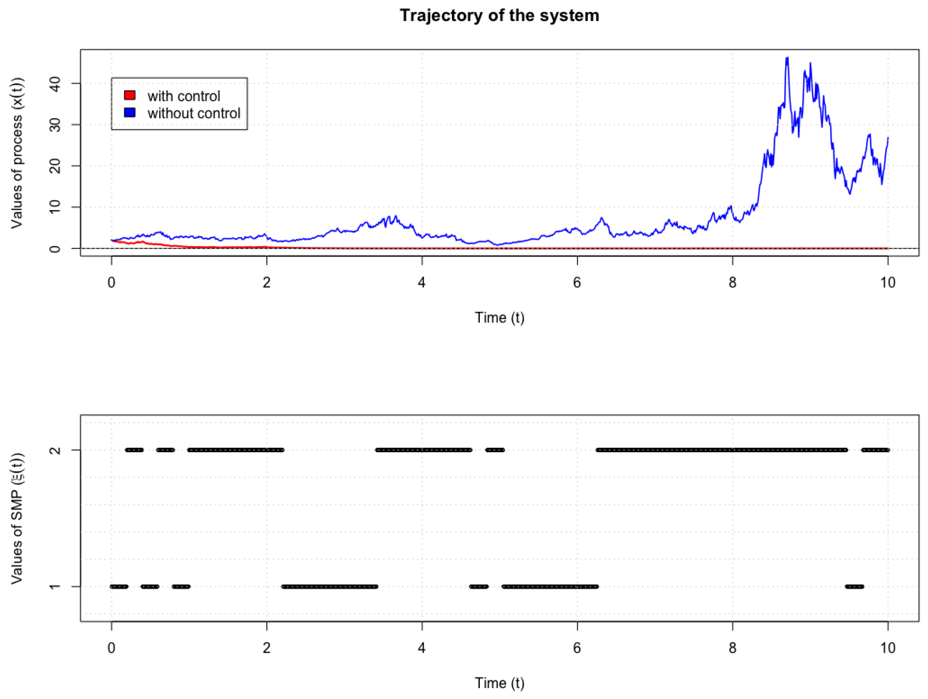
The realization of the solution of the system (46)–(47) without control and under the influence of optimal control is shown in Figure 1.

Figure 1. Solution of the system (46)–(47) with the given values of the coefficients.

8. Discussion

The main focus of this paper is on theoretical derivations of the optimal control system for stochastic differential equations in the presence of external perturbations described by semi-Markov processes. This generalization allows us to more accurately describe the dynamics of real processes under various kinds of restrictions on the spend time

$θ_{n}$ in states, which is impossible in the case of a Markov process. In Theorem 2, we find an explicit form of the infinitesimal operator, which is determined on the basis of the coefficients of the original equation and the characteristics of the semi-Markov process. This representation allows us to synthesize the optimal control

$u^{0} (t, x)$ based on the Belman equation (18) with the boundary condition (19). For the linear case of the system of the form (30), the search for optimal control is carried out on the basis of solving the Riccati equation (39), which also arises in the case of the presence of a Markovian external perturbation.

The main focus in the following works for dynamical systems with semi-Markovian external perturbations will be on taking into account the ergodic properties of the semi-Markovian process

$ξ (t), t \geq 0$ when analyzing the asymptotic behavior of the system. In contrast to systems with Markovian external switches, where the ergodic properties of

$ξ (t)$ were described on the basis of intensities

$λ (y)$ , for the semi-Markovian case, conditions on the times of steady-state and jumps will play an important role. Thus, the parameter estimate of model (2) will have not only an estimate of the parameters

$a (\cdot), b (\cdot)$ , but also an estimate of the distribution of the residence time in the states. Therefore, the following algorithm can be proposed for system analysis and parameter estimation:

Estimation of switching moments

$τ_{n} = \sum_{i = 1}^{n} θ_{n};$

This estimation can be realized using a generalized unit root test developed for time series [16];
Estimation state spase for semi-Markov process $ξ (t)$ ,

$Y = {1, 2, . . ., N};$
Estimation coefficients $a (\cdot), b (\cdot)$ for SDE (2);

The presented framework of stochastic dynamic systems with semi-Markov parameters offers a promising tool for systems biology and systems medicine. In systems biology, it can help model complex molecular interactions, such as oxidative stress and mitochondrial dysfunction, influenced by stochastic perturbations. In systems medicine, this approach supports personalized treatment strategies by capturing patient-specific dynamics. For instance, it can predict disease progression and optimize therapies in conditions like Parkinson’s Disease. By integrating theoretical modeling with clinical data, this framework bridges the gap between understanding disease mechanisms and advancing precision medicine.

9. Conclusions

In this paper, we solve the problem of synthesis of optimal control for stochastic dynamical systems with semi-Markov parameters. In the linear case, an algorithm for finding the optimal control is obtained and its convergence is substantiated.

[custom]

Funding

This research was supported by ELIXIR-LU https://elixir-luxembourg.org/, the Luxembourgish node of ELIXIR, with funding and infrastructure provided by the Luxembourg Centre for Systems Biomedicine (LCSB). LCSB’s support contributed to the computational analyses and methodological development presented in this study.

Acknowledgments

The authors would like to acknowledge the institutional support provided by the Luxembourg Centre for Systems Biomedicine (LCSB) at the University of Luxembourg and Yuriy Fedkovych Chernivtsi National University, which facilitated the completion of this work.

Conflicts of Interest

The authors declare no conflicts of interest.

References

Lindquist, A. Optimal control of linear stochastic systems with applications to time lag systems. Information Sciences 1973, 5, 81–124. [Google Scholar] [CrossRef]
Kumar P., R.; van Schuppen J., H. . On the optimal control of stochastic systems with an exponential-of-integral performance index. Journal of Mathematical Analysis and Applications, 1981; 80, 312–332. [Google Scholar]
Buckdahn, R.; Labed, B.; Rainer, C.; Tamer, L. Existence of an optimal control for stochastic control systems with nonlinear cost functional. Stochastics 2010, 82(3), 241–256. [Google Scholar] [CrossRef]
Dragan, V.; Popa, I.-L. The Linear Quadratic Optimal Control Problem for Stochastic Systems Controlled by Impulses. Symmetry 2024, 16, 1170. [Google Scholar] [CrossRef]
Das, A.; Lukashiv, T. O.; Malyk, I. V. Optimal control synthesis for stochastic dynamical systems of random structure with the markovian switchings. Journal of Automation and Information Sciences 2017, 4(49), 37–47. [Google Scholar] [CrossRef]
Antonyuk, S. V.; Byrka, M. F.; Gorbatenko, M. Y.; Lukashiv, T. O.; Malyk, I. V. Optimal Control of Stochastic Dynamic Systems of a Random Structure with Poisson Switches and Markov Switching. Journal of Mathematics 2020. [Google Scholar] [CrossRef]
Dynkin, E.B. Markov Processes; Academic Press: New York, USA, 1965. [Google Scholar]
Koroliuk, V.; Limnios, N. Stochastic Systems in Merging Phase Space; World Scientific Publishing Co Pte Ltd: Hackensack, NJ, USA, 2005. [Google Scholar]
Ibe, O. Markov Processes for Stochastic Modelling. 2nd Edition; Elsevier: London, UK, 2013. [Google Scholar]
Gikhman, I. I.; Skorokhod, A. V. Introduction to the Theory of Random Processes; W. B. Saunders: Philadelphia, PA, USA, 1969. [Google Scholar]
Øksendal, B. Stochastic Differential Equation. Springer: New York, USA, 2013.
Kolmanovskii V., B.; Shaikhet L., E. Control of Systems with Aftereffect; American Mathematical Society: Providence, RI, USA, 1996. [Google Scholar]
Jacod, J.; Shiryaev, A. N. Limit Theorems for Stochastic Processes. Vols. 1 and 2; Fizmatlit: Moscow, Russia, 1994. (in Russian) [Google Scholar]
Lukashiv, T. One Form of Lyapunov Operator for Stochastic Dynamic System with Markov Parameters. Journal of Mathematics 2016. [Google Scholar] [CrossRef]
Bellman, R. Dynamic Programming; Princeton University Press: Princeton, NJ, USA, 1972. [Google Scholar]
Narayan, P.; Popp, S. A New Unit Root Test with Two Structural Breaks in Level and Slope at Unknown Time. Journal of Applied Statistics 2010, 37, 1425–1438. [Google Scholar] [CrossRef]

Disclaimer/Publisher’s Note: The statements, opinions and data contained in all publications are solely those of the individual author(s) and contributor(s) and not of MDPI and/or the editor(s). MDPI and/or the editor(s) disclaim responsibility for any injury to people or property resulting from any ideas, methods, instructions or products referred to in the content.

© 1996 by the authors. Licensee MDPI, Basel, Switzerland. This article is an open access article distributed under the terms and conditions of the Creative Commons Attribution (CC BY) license (https://creativecommons.org/licenses/by/4.0/).

Copyright: This open access article is published under a Creative Commons CC BY 4.0 license, which permit the free download, distribution, and reuse, provided that the author and preprint are cited in any reuse.

Downloads

Views

Comments

Subscription

Notify me about updates to this article or when a peer-reviewed version is published.

MDPI Initiatives

Important Links

Choose an area of interest and we will send you notifications of new preprints at your preferred frequency.

Disclaimer

Optimal Control of Stochastic Dynamic Systems with Semi-Markov Parameters

Abstract

Keywords:

Subject:

1. Introduction

2. Problem Statement

3. Sufficient Conditions for Optimality

4. General Solution of the Optimal Control Problem

5. Synthesis of Optimal Control for a Linear Stochastic System

6. Construction of the Bellman Equation

7. Model Example

8. Discussion

9. Conclusions

Funding

Acknowledgments

Conflicts of Interest

References

MDPI Initiatives

Important Links

Subscribe