Multi Energy Static Modelling Approaches: A Critical Overview

1. Introduction

In the last years, decarbonization has become one of the most important imperatives in the energy sector. The European Union, as well as many other Countries in the world, have set very ambitious climate-neutrality targets for the mid-long term ([1]). In the electricity sector, this produced an important increase in the deployment pace for the so-called Renewable Energy Sources (RES), most notably wind and solar. At the same time, traditional big generators, based on fossil-fuels, are being more and more decommissioned because out of merit order in the electricity markets and not any longer compliant with the environmental targets. This trend has been reinforced and even more accelerated in the last years, when important geo-political events have put the accent on security of supply and on making the energy system independent from the purchase of fuels from politically unstable or critical nations. However, for the electricity system, characterized by a very limited intrinsic flexibility (as electrochemical batteries can provide only limited storage capabilities and demand-side involvement stays rather limited), substantially increasing the penetration of RES, typically characterized by variable generation patterns, means the need to procure more and more services, for congestion management, frequency control, etc. RES power plants are characterized by evident generation peaks and valleys and if electricity transmission and distribution networks were reinforced for hosting such peaks without causing congestion, this would call for very expensive refurbishment actions, against, maybe, a very limited number of hours during the year in which such expanded grids would be fully utilized. In these cases, grid expansion would prove economically unjustified.

The same decarbonization targets mentioned above push also in the direction of an overall electrification of power consumption, in the industrial sector as well as for energy end-uses. However, not all industrial processes can easily be electrified, and some industrial sectors (cement, paper) are hardly electrifiable with the present technologies, or, in other cases (steel), could be electrified only by completely replacing the present production technologies, thus by carrying out huge investments. These sectors, usually called hard-to-abate, alongside with the heavy transport sector, although not easily electrifiable, could be fed with other energy vectors, most notably hydrogen. As a matter of fact, hydrogen ([2]) is imposing itself as one of the most promising decarbonization “tiles” of future energy policies. However, green hydrogen is produced through electrolysers which are, in turn, using electricity in great quantities, hence again the need to expand the electricity grid.

To cope with the very limited storage capability of the electricity system, other carriers could prove very helpful. Natural gas is characterized by very high compressibility (this phenomenon is called linepack) and there is a wide range of admissible operative pressures. Thus, the entire gas network, tightly coupled to the electricity network, could be exploited to provide flexibility to the electricity vector itself, as it were a huge, distributed storage system.

Hydrogen storage is itself very promising: both for short term storage (able to compensate daily peaks of RES electric generation) and even for long term storage (able to compensate important seasonal generation differences of wind and solar power plants). Hydrogen storage and flow-batteries are deemed as the only presently mature technologies for long term storage.

Finally, heat networks show an important flexibility potential too: thermal systems, be they those of small-scale swimming pools ([3]) or much larger ones for district-heating ([4]), can guarantee acceptable levels of comfort if water temperatures are held within given wide operative ranges and this flexibility can, again, be exploited to the advantage of the electricity carrier to which services can be provided.

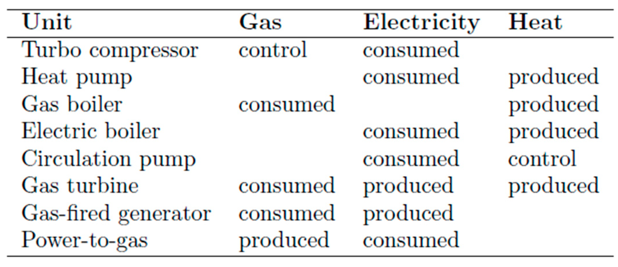
Table 1 summarizes the most typical interactions between the energy carriers and the devices (“units”) where the energy conversion processes between carriers take place.

All the above reasons motivate an extension of the traditional scenario simulations and planning studies for the electric system by including other carriers (natural gas, hydrogen, district-heating) with which the electricity system is (and will be more and more in the future) interconnected. Regarding dispatch scenario studies, the addition of the other interconnected carriers can help to achieve a more optimized equilibrium and a better quantification of the interdependences between the different carriers. Concerning planning studies, considering the mutual interdependency of the different sectors can help to exploit synergies and spare refurbishment costs which are economically unjustified. Additionally, electric grids expansion meets more and more opposition from the public opinion, and this impacts on very long approval times which heavily contrast with the rapidity needed to deploy all that is needed to comply with current decarbonization targets and deadlines. Thus, reducing the number of grid refurbishment interventions by exploiting synergies between carriers in a holistic approach is also a way to ease and speed up the realization of the needed electric grid upgrades.

The above considerations on the importance to adopt a Multi Energy (ME) approach in dispatch scenarios and planning studies is also reflected in numerous policy documents, which clearly call for the adoption of a multi-carrier approach. Just to mention a couple of them, at European Union level, the European Commission ([6]) published already in 2020 the Communication “Powering a climate neutral economy: an EU Strategy for energy system integration” ([7]). In this document, we find “Energy system integration – the coordinated planning and operation of the energy system ‘as a whole’, across multiple energy carriers, infrastructures, and consumption sectors – is the pathway towards an effective, affordable and deep decarbonisation of the European economy”. The more recent document “Electricity infrastructure development to support a competitive and sustainable energy system - 2024 Monitoring Report” ([8]) published by the European Union Agency for the Cooperation of Energy Regulators (ACER, [9]) invites grid developers “to extend the use of multi-vector scenarios to grid development planning at the national level and ensure consistency between EU TYNDP and national scenarios”. Finally, the European Network of Transmission System Operators for Electricity (ENTSO-E, [10]) and the European Network of Transmission System Operators for Gas (ENTSOG, [11]) have recently started to publish joint electricity-gas scenarios to support the vision of the Ten-Year-Network-Development-Plan 2024. These scenarios are publicly available on the web ([12]). While introducing such scenarios, ENTSO-E and ENTSOG declare “The scenarios evaluate the interactions between the gas, hydrogen and electricity systems, vital to delivering the best assessment of the infrastructure from an integrated system perspective”.

So, it is no surprise that the last years have seen the birth of a new research line, consisting in the development of ME static models, i.e. those that are suitable for carrying out dispatch studies as well as planning analyses. Both have in common the static description of the different carriers (as opposed to the one oriented to study transient phenomena) and the fact that very often they imply either the solution of a system of equations for the calculation of power flows once the input-output quantities are known (the so-called ”load-flow” problems) or the resolution of very large optimization systems that minimize OPerative system EXpenditures (OPEX, very often in the sense of pure dispatching costs) or the TOTal system EXpenditures (TOTEX, meant as the sum of OPEX and CAPEX for investing in new assets to be deployed). The peculiarity of these models, if applied in a ME context instead of a single energy carrier, is that the dimension of the problem is considerably larger. This means that particular attention should be paid on one side to find out the simplest schematization of the single components of each carrier (e.g. preserving the linearity of the models becomes nearly imperative) and on the other side to utilize opportune solving algorithms fit for managing very large systems and most likely utilizing modern decomposition techniques (like Benders’ decomposition [13]).

This paper concentrates only on modelling issues and does not treat algorithms and techniques fit to solve the very large mathematical models generated in this way. After the present introduction, the second chapter will describe in synthesis the most significant modelling aspects for the main components of the carriers to be typically considered in a ME model: electricity, gas, hydrogen and heat. The third chapter will deal with the most typical techniques for joining the different carriers in one simulation model. Here, the goal is not to be exhaustive by quoting every single paper that has been produced in the last years (it would be nearly impossible!), but, rather, to single out the most typical approaches and to outline the peculiarities for each of them. Finally, the conclusive chapter will provide a comparison of the different approaches and some advice for those interested in ME modelling. The style of the paper is that of a tutorial aimed at providing some guidance and a few bibliographic references to those who are interested to get a first approach to ME modelling.

2. Energy Carriers Static Modelling Approaches

Before discussing the most common ME modelling approaches, it is opportune to carry out an analysis of the mathematic models of the main components of each carrier. In this analysis we are going to start from the general approaches and then indicate which simplifications can be useful to make the model fit for simulating large scale systems (i.e. networks with a few thousand nodes for each carrier). To this aim, the most important factors to be preserved are model convexity and model linearity. Model convexity ([14]) ensures that an optimization problem has one only solution and it is, thus, not subject to local minima, which may typically constitute a serious problem, making numerical convergence more difficult to achieve and potentially making solutions found for subsequent time instants not mutually comparable. Linear optimization models are also convex. Linearity is an essential prerequisite to apply algorithms like the interior point ([15]), which are both very fast and powerful to deal with large scale systems. Bearing in mind that planning problems are typically modelled as mixed integer (investments are typically associated to binary variables, see e.g. the model developed by the FlexPlan European research project [16]), the fact of solving Mixed Integer Linear Problems (MILP, [17]) brings huge advantages with respect to solving Mixed Integer Non-Linear Problems (MINLP).

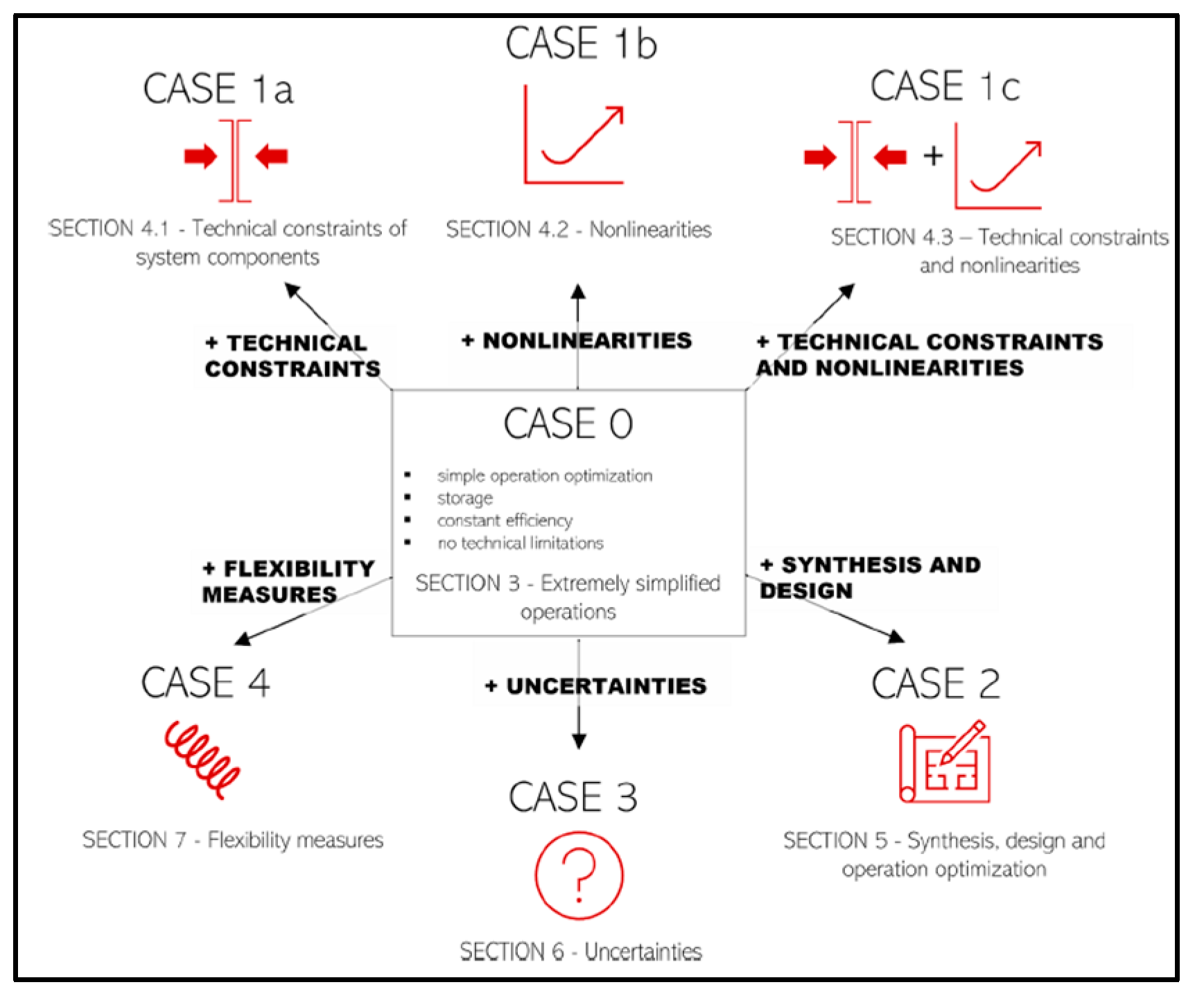
In general, and for Multi Energy Systems (MES) even more, model complexity is a function of the detail adopted in the representation of each system component. More detail on components behavior implies a more complex mathematical description. So, it is of paramount importance to understand which is the best compromise between completeness of the mathematical representation of the system and complexity of the resulting problem (which implies the kind of solver which can be used and the time of resolution or, in many cases, just whether the problem is numerical tractable with the present hardware and software or not). From this point of view, [18] provides an interesting classification of the mathematical representation (and complexity) associated with the different modelling details treated in ME models. ME models are divided into 7 categories (Figure 1). Table 2 shows the typical modelling criticalities of each category.

As it is evident by examining in Table 2, mathematical complexity increases with the realism of the model and the number of included details (components non-linearity, technical constraints, uncertainty, flexibility and ancillary services) and considerably changes with the aim of the model (only dispatch variables for optimization of short time system operation, also investment variables, which are typically integer ones, for long time grid design and planning).

The following sections will examine the main peculiarities of the static models describing the components of different carriers (electricity networks, compressible fluid networks and heat networks). Among them, compressible fluids networks, which can represent either natural gas or hydrogen networks, and heat networks are the most complicated cases, because the relevant equations are not easily linearized without committing important approximations and because the approaches for static modelling are less established than for the electricity networks. Albeit simplifications are carried out in nearly all approaches to model multi-carrier networks, it is important to have a look at the general case and analyze the meaning of the different approximations to be brought in order to get to a linear model. For this reason, the section dedicated to compressible fluid networks is much longer than the ones dedicated to the other two carriers.

Electricity networks modelling

Electricity networks are included in plenty of simulation tools and applications and the relevant modelling approach necessary for each domain of simulation (planning, operation, contingency analysis, etc) is well known. There also exist some very known open access libraries, which can be used as a basis to build simulation tools: just to mention some of the most known ones, MATPOWER ([21]) for the MATLAB programming language ([22]). and PowerModels ([23]) for the Julia programming language ([24]). Nonetheless, the brief introduction provided by the present section is necessary both for the sake of completeness with respect to what is written for the other energy carriers and to provide an overview of the most common modelling choices with specific reference to static models. For a more complete introduction to the modelling of the electric networks, the reader is sent to dedicated books (a few bibliographic references can be found in [25]).

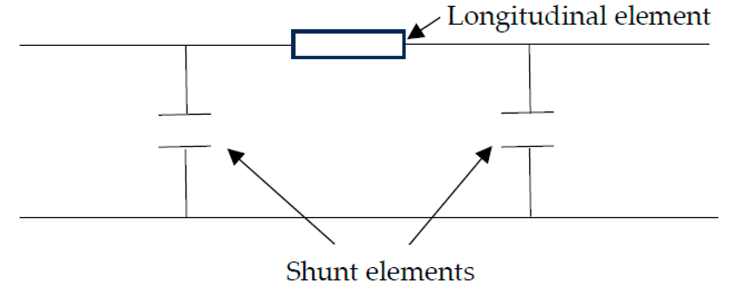
Starting from electrical lines, active and reactive power can be calculated for each branch of the network by utilizing the following simplified formulation (after neglecting the shunt part of the π model, see Figure 2):

$$p_{hk}=V_h{V}_k\left[g_{hk}\cos \left({\theta }_h-{\theta }_k\right)+b_{hk}\sin \left({\theta }_h-{\theta }_k\right)\right]$$

(1)

$$q_{hk}=V_h{V}_k\left[g_{hk}\sin \left({\theta }_h-{\theta }_k\right)-b_{hk}\cos \left({\theta }_h-{\theta }_k\right)\right]$$

(2)

where p_hk is the active power of the branch between nodes h and k, q_hk is the reactive power between the same nodes, V_h and V_k are the voltage modules for the two nodes h and k, and θ_h and θ_k the voltage angles for the same nodes, g_hk and b_hk are, respectively, the real part and the imaginary part of the admittance y_hk of the branch between nodes h and k.

The equations system constituted by (1) and (2) is non-linear and this can be an important drawback to execute studies over big networks (even bigger if other carriers are added) and over long-term time intervals (which is typical, e.g. for grid planning analyses). On the other side, the longitudinal reactance of the transmission networks lines is usually much bigger than the relevant resistance (for 150kV networks, this ratio can be around 1.7, whereas for 380kV networks the same can increase up to 10). In this hypothesis, being the transversal (shunt) impedances of reactive type, they don’t influence active power transits, and the expressions for active and reactive power calculation are decoupled. Thus, by considering only equation (1) for active power calculation, it becomes:

$$p_{hk}=V_h{V}_k{b}_{hk}\sin \left({\theta }_h-{\theta }_k\right)={\displaystyle \frac{V_h{V}_k}{x_{hk}}}\sin \left({\theta }_h-{\theta }_k\right)$$

(3)

where x_hk is the reactance between nodes h and k. Moreover, as reactive flows are not of interest, the voltage modules at the two extremes of the line can be considered equal and approximated with their nominal value V_n. Finally, the difference (θ_h - θ_k) is typically small and thus the sine is approximately equal to its argument. Hence:

$$p_{hk}={\displaystyle \frac{{V_n}^2}{x_{hk}}}\left({\theta }_h-{\theta }_k\right)$$

(4)

which is a linear expression that can be put in matrix form and solved with the customary numerical algorithms in order to calculate the system load low once active power injections are known. This linearized representation in current denominated direct current approximation of the load flow equations.

For distribution networks, the hypothesis that longitudinal reactance of lines is usually much bigger than the relevant resistances doesn’t hold, and, thus, the direct current approximation cannot be made. However, for distribution networks the DISTFLOW approach can be adopted. Such approach retains an approximate calculation of reactive power alongside active power by applying opportune approximations so that the final solving system stays linear (for details, see [26,27]).

In alternative to applying the direct current approximation, a different kind of linear representation can be adopted. This representation is based on the so-called Power Transfer Distribution Factors (PTDF), defined as the incremental change in the active power that flows in a transmission line l due to an active power injection in a given node n of the network. PTDF factors provide a linearized description of the modalities how flows on the transmission lines change in response to extra injections into the system. The most important information they synthetize is how active power flows split among parallel branches of a meshed transmission network as an effect of the different impedances of the branches themselves. In a meshed transmission network, PTDF factors can take whatsoever value between zero and one, the former meaning that an injection into node n doesn’t affect at all line l, the latter that the entire flow injected into n transits through l. Of course, PTDF factors of distribution networks, having a tree topological structure, can be only either equal to zero or to one. PTDF are usually collected into a bidimensional matrix having so many rows as the number of lines and as many columns as the number of nodes. Theoretically, the PTDF matrix can be calculated starting from the inverse of the impedance matrix ([28]). However, typically, PTDF factors are calculated by running sensitivity simulations on the studied system scenarios. Once the PTDF matrix is calculated, PTDF factors are used in the system constraint that enforces the transit limits for each line:

$$I_{ml}\le {\displaystyle \sum }_{n\in N}\left[{\sigma }_{ln} \left({\displaystyle \sum }_{g\in n}{p}_g-{\displaystyle \sum }_{c\in n}{C}_c\right)\right]\le I_{Ml}$$

(5)

where I_ml and I_Ml are, respectively, the minimum and maximum limits for active power in line l, p_g and C_c are the generic generator and load in node n, σ_ln the PTDF factor between node n and line l.

Regarding the PTDF representation, it must be noted that it works well if the topology of system to be studied is fixed (e.g. to calculate system dispatch, e.g. electric markets outcome). By contrast, this representation can’t be easily applied to grid planning studies, since including more lines modifies the ratios between the impedances of the single lines, thus the relevant PTDF factors.

Electrochemical batteries are important components of present electrical grids. The simplest way to model them is through the following equation:

$$E_{t+1}=E_t+\left({\eta }^{abs}{P_t}^{abs}-{\displaystyle \frac{{P_t}^{inj}}{{\eta }^{inj}}}+{\xi }_t\right)\Delta t$$

(6)

where E_t and E_t+1 are the amount of energy stored in the battery at time t and t+1, Δt is the time interval between t and t+1, P_t^abs and P_t^inject are the amount of power absorbed and injected at time t, η^abs and η^inj are the efficiencies in absorption and injection and ξ_t is a possible exogenous term (e.g. a self-discharge factor).

This kind of equation is an integral constraint, binding the energy (state variable) at time t+1 with energy at time t. Integral constraints increase the number of non-zeros in the Jacobian matrix ([29]) and make simulations more numerically demanding.

The model written in (6) can be made much more complex: extra constraints can be introduced to represent maximum charge, maximum power ramp-up and down, capacity reduction of the equipment as a result of the number of charge-discharge cycles it has been subjected to ([30]) and other. As usually, a compromise between completeness and realism must be sought for in order to ensure numerical tractability while including the effects that are important for the study to be accomplished. Very large models for planning studies suggest reducing to the minimum the number of treated constraints while ensuring that the resulting model, yet maybe including integer variables, stays linear.

Compressible fluids modelling

Natural gas networks are tightly connected to electrical networks (gas-fired thermoelectrical plants consume natural gas to produce electricity; synthetic gas blended into gas networks is produced using electricity; gas linepack can provide flexibility to the electricity sector) and future hydrogen networks will be closely connected as well (green hydrogen is produced with electrolysers which consume electricity; fuel cells convert hydrogen storage into electricity). This justifies modelling the two carriers together and, what concerns grid planning studies, even to put in competition the planning policies of the two networks. However, as already pointed out, natural gas networks modelling (or, in general, compressible fluids flow modelling) is rather complicated and non-linear. Nonetheless, linearization procedures can be adopted as well.

As the elementary building block of a gas network, we will limit ourselves to describe the modelling of an isothermal pipeline as it can be found in [31], i.e. adopting the hypothesis that the gas temperature is constant throughout the duct and equal to the external one (T(x,t) = T_E, where x is an abscissa along the length of the pipeline and t is the temporal coordinate). A much more complicated modelling approach ([32]) removes this simplification and explicitly models the exchange of energy with the external environment though the pipeline metal structure: this model is, however, relevant only for transient studies. Further assumptions to be made to model an isothermal pipeline are:

• turbulent motion in the pipeline (this is always verified for gas transport pipelines at a distance equal to some multiples of the diameter from the beginning and the end of the duct). This allows to adopt a mono-dimensional description for the fluid motion equations (otherwise, the Navier-Stokes [33] fluid dynamics laws should be used),
• the pipeline is regular: there are neither changes of section along x nor sharp changes of direction (curves): such cases are usually modelled through concentrated losses (i.e. a pressure reduction), proportional to the square of the fluid speed through a coefficient depending on the type of irregularity),
• the perfect gas law holds:

$${\displaystyle \frac{p\left(x,t\right)}{\rho \left(x,t\right)}}=z{R}_{G}T\left(x,t\right)$$

(7)

where p is the pressure, ρ is the gas density, z is the gas compressibility factor and R_G is the gas constant. Starting from (7), the sound speed C can be defined as:

$${{\displaystyle \frac{\partial \rho }{\partial p}}|}_{T=T_E}={\displaystyle \frac{1}{C^2}}={\displaystyle \frac{1}{z{R}_G T_E}}\to C=\sqrt{z{R}_G T_E}$$

(8)

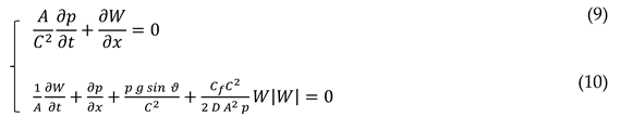
In these hypotheses, the mass and momentum conservation laws become:

where A is the pipe section, W is the gas mass flow rate, g is the gravity constant, θ is the line slope with respect to horizontal, C_f is the friction coefficient and D is the pipe diameter. By equaling to zero the time derivatives, one gets:

• W(x)= constant, i.e. mass flow rate constant throughout the pipeline,
• the following expression for pressure drop calculation:

$$P_1-P_2={\displaystyle \frac{ C_f{C}^2\Delta x}{\left(p_1+p_2\right)D A^2}}{\displaystyle \frac{e^s-1}{s}}W\left|W\right|+{\displaystyle \frac{{p_{2 }}^2}{\left(p_1+p_2\right)}}\left(e^s-1\right)$$

(11)

where: $s={\displaystyle \frac{g \Delta x \sin \vartheta }{2 C^2}}$. If the pipeline is horizontal (θ = 0), the equation becomes:

$$W\left|W\right|={\displaystyle \frac{D A^2}{C_f{C}^2\Delta x}}\left(p_1^2-p_2^2\right)=K\left(p_1^2-p_2^2\right)$$

(12)

This relationship, usually called Weymouth equation, is the most typically used one in the modelling of pressure drops along gas pipelines in steady state disregarding the gravitational effect (customary hypothesis when simulating large gas networks). Equation (12) is not linear, but linearization procedures can be applied, as described in [34].

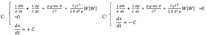
The Weymouth equation is useful to calculate pressure drops in the pipelines of a gas network. However, another important aspect, which is the delay due to the limited propagation speed of a perturbation in a gas duct, is not considered by the above steady state equation. This aspect is not negligible, especially when considering very long gas backbones crossing whole Europe. In order to consider it, we must re-elaborate the non-stationary equation set (9) (10). The most common approach is constituted by the so-called method of the characteristics. In order to derive such method, let’s create a linear combination of equation (9), denominated L1 and (10), denominated L2:

$$L=\lambda L_1+L_2={\displaystyle \frac{1}{A}}\left[\lambda C^2{W}_x+W_t\right]+\lambda \left[{\displaystyle \frac{1}{\lambda }}{p}_x+p_t\right]+{\displaystyle \frac{pgsin\vartheta }{C^2}}+{\displaystyle \frac{C_f{C}^2}{2D{A}^{2}p}}W\left|W\right|=0$$

(13)

In order to be able to interpret the two quantities in square bracket as total time derivatives of, respectively, W and P, the following equalities must hold:

$${\displaystyle \frac{dx}{dt}}={\displaystyle \frac{1}{\lambda }}=\lambda C^{2 }\mathrm{hence}\lambda =\pm {\displaystyle \frac{1}{C}}$$

(14)

By replacing (14) in (13), we obtain two systems of differential equations, which must be satisfied at the same time:

(15)

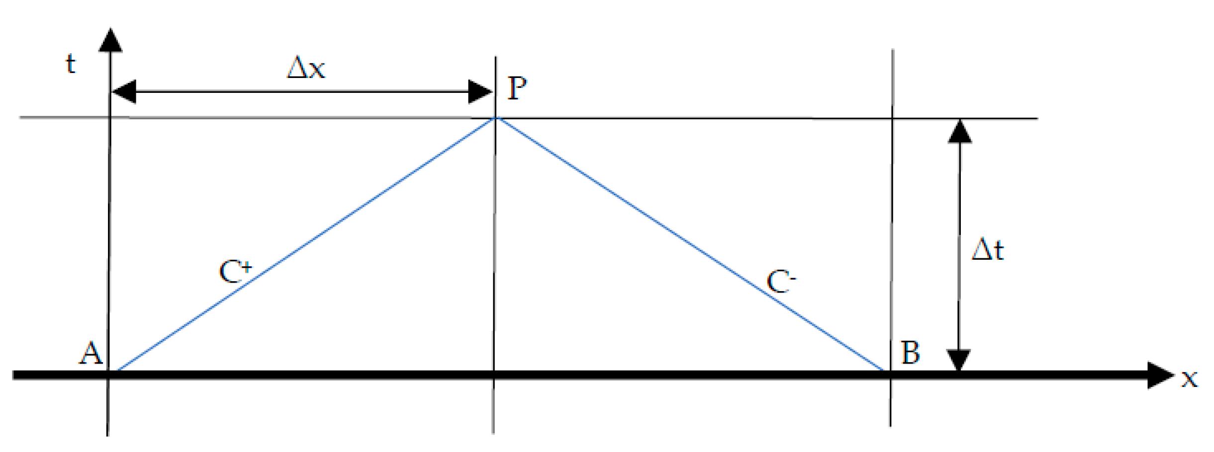
By integrating these two systems, we obtain the following two relationships:

$${\displaystyle \frac{C}{A}}\left(W_P-W_A\right)+\left(p_P-p_A\right)+{\displaystyle \frac{C_f{C}^2\Delta x}{\left(p_P+p_A\right)D A^2}}{\displaystyle \frac{e^s-1}{s}}{\displaystyle \frac{W_P+W_A}{2}}\left|{\displaystyle \frac{W_P+W_A}{2}}\right|+{\displaystyle \frac{{p_{P }}^2}{\left(p_P+p_A\right)}\left(e^s-1\right)=0}$$

(16)

$${\displaystyle \frac{C}{A}}\left(W_P-W_A\right)-\left(p_P-p_B\right)+{\displaystyle \frac{C_f{C}^2\Delta x}{\left(p_P+p_B\right)D A^2}}{\displaystyle \frac{e^s-1}{s}}{\displaystyle \frac{W_P+W_B}{2}}\left|{\displaystyle \frac{W_P+W_B}{2}}\right|+{\displaystyle \frac{{p_{B }}^2}{\left(p_P+p_B\right)}}\left(e^s-1\right)=0$$

(17)

which must be satisfied at the same time, (16) along the line with slope +C and (17) along a line with slope -C (the two characteristic lines), see Figure 3. Once the W and p values are calculated for time t, for each couple of grid points A and B, the same quantities can be calculated at time t+Δt for point P by solving the system of equations (16) and (17).

The method of the characteristics is convergent (“stable”) provided that the spatial grid points and the discretization of the time axis are chosen so that the Friedrichs-Courant-Lewy ([35], [36]) equation is satisfied:

(18)

The intuitive interpretation of this relationship is that, after splitting the length of the pipeline in equally spaced grid points at distance Δx, the equally spaced time steps spacing Δt must be chosen so that it is not bigger than the time taken by progressive and regressive waves (along, respectively, C⁺ and C^-) to cover the distance Δx.

The method of characteristics, i.e. solving the set of equations (16) and (17), allows to calculate mass flow rate and pressure drops along a pipeline with a very good level of approximation (the isothermal duct hypothesis, true except for fast transients, being the only important applied precondition). However, these relationships are strongly non-linear, and the Friedrichs-Courant condition (18) imposes a very tight time discretization. On top of that, the values at time t+1 are iteratively calculated only once all values at time t have already been calculated: in case of an optimization process (e.g. for planning models) this means that all equations for all points of the discretized spatial grid and along the entire time horizon of the simulation must be written and solved altogether. All these issues limit the concrete possibility to apply this methodology to large static models, which, usually, just use the Weymouth equation formulation (12) or its linearized version.

Linearized formulations for the solving problem of the gas flow equations (9)(10) do exist. One of the most interesting ones can be found in [37]. It applies a finite differences method to a pre-determined spatial-temporal grid and a Taylor series linear approximation in order to get to a linear discretized model. However, this model doesn’t guarantee to preserve the speed of propagation of pressure waves (since the spatial-temporal grid is selected without caring about the slope of the characteristic curves C⁺ and C^-). Additionally, the values in (x+Δx, t+Δt) are iteratively calculated by taking as known all values at the previous time step as well as those at the present time step for the spatial points which precede the one being calculated. So, as it was the case for the methodology of the characteristics this means that, in case of an optimization process (e.g. for planning models), the full equations set must be written and solved altogether, for all points of the discretized spatial grid and along the entire time horizon of the simulation. This makes this model hardly suitable for large static models.

Apart the non-linear modelling of the gas pipelines, other two important components, centrifugal compressors and regulation valves, show non-linear behaviors, and this must be seriously accounted for, especially when dealing with large static models and within large optimization procedures (e.g. for grid planning).

Compressor stations are installed along gas networks to boost pressure to ensure proper delivery. Compressor stations are pumping stations consisting of multiple compressor units, scrubber, cooling facilities, emergency shutdown systems, and an on-site computerized flow control and dispatch system that maintain the operation of the system. These stations are usually coupled with gas turbines which consume part of the transported gas for operation. It is estimated ([38]) that such stations consume 3-5 % of the gas and constitute 20% of the total operating cost of the company. The equation describing the functioning of a gas centrifugal compressor is (see [39]):

$$H=z{R}_{G}T{\displaystyle \frac{k}{k-1}}\left[{\left({\displaystyle \frac{p_d}{p_s}}\right)}^{{\displaystyle \frac{k-1}{k}}}-1\right]$$

(19)

where H is the compressor prevalence, z is the gas compressibility factor, R_G is the gas constant, k is the isentropic exponent ([39]), p_d and p_s are, respectively the discharge and suction pressures. Prevalence H and mechanical power P required to compress the gas in the compressor are bound by:

$$WH={\eta }_{is}P$$

(20)

where W is the gas mass flow rate and η_is is the thermodynamical efficiency.

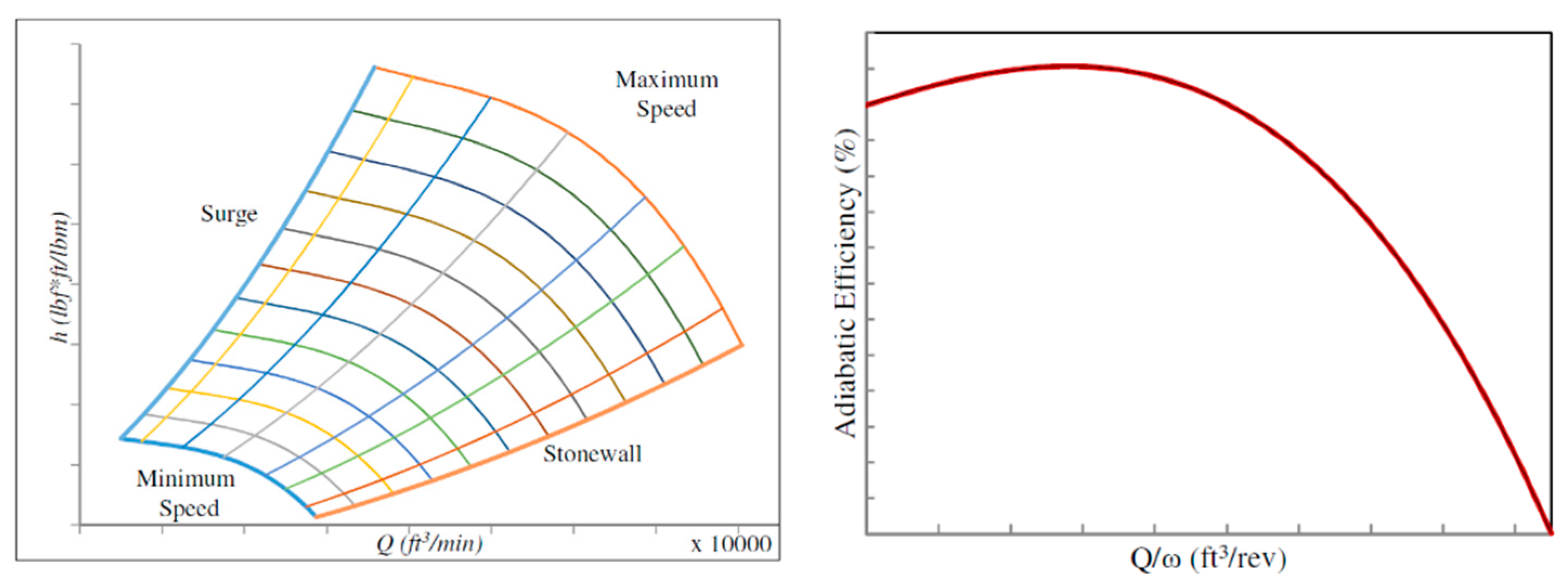
Compressors have to operate within established limits, which are plate data of each device. A natural way to characterize the performance of centrifugal compressors is in terms of the inlet volumetric flow rate, speed, adiabatic head, and adiabatic efficiency. The relationships between these quantities are usually represented by performance maps (see Figure 4) which are plots of H and as functions of Q (volumetric flow rate) at different speeds. These performance maps can be approximated by cubic polynomial functions with constant coefficients, fitted by using the least squares method ([40]):

$${\displaystyle \frac{H}{{\omega }^2}}=A_H+B_H\left({\displaystyle \frac{Q_s}{\omega }}\right)+C_H{\left({\displaystyle \frac{Q_s}{\omega }}\right)}^2+D_H{\left({\displaystyle \frac{Q_s}{\omega }}\right)}^3$$

(21)

$${\eta }_{is}=A_E+B_E\left({\displaystyle \frac{Q_s}{\omega }}\right)+C_E{\left({\displaystyle \frac{Q_s}{\omega }}\right)}^2+D_E{\left({\displaystyle \frac{Q_s}{\omega }}\right)}^3$$

(22)

where Qs is the volume flow rate at surge and ω is the rotational speed (to be limited between minimum and maximum values).

Regulation valves are another important element of gas networks, and they show a strongly non-linear behavior ([32]) too. They are constituted by a convergent section following by a divergent section. In the convergent section, the laws of conservation of momentum (written by ignoring the terms of accumulation, friction, gravity) and mass are valid. Furthermore, the transformation is considered isentropic. Velocity increases in the convergent but can at most reach the sonic speed. The relationship between mass flow rate (W) and the initial and final pressures in the convergent (respectively, p₁ and p₂) is:

$$W=A_{st} \chi \left({\displaystyle \frac{p_2}{p_1}}\right)\sqrt{{\rho }_1{p}_1}\mathrm{where}{\displaystyle \frac{p_2}{p_1}}\ge r_c\approx 0.528\mathrm{and}{r}_c={\left({\displaystyle \frac{2}{\gamma +1}}\right)}^{{\displaystyle \frac{\gamma }{\gamma -1}}}$$

(23)

where r_c is the pressure ratio in the sonic case, ρ₁ the upstream fluid density and the isentropic coefficient A_st is the smallest section area. The χ function is defined as follows:

$$\chi \left(\beta \right)={\displaystyle \frac{2\gamma }{\gamma -1}}{\displaystyle \frac{{\beta }^{\frac{2}{\gamma }}-{\beta }^{\frac{\gamma +1}{\gamma }}}{1+{\alpha }_A^2{\beta }^{\frac{2}{\gamma }}}}$$

(24)

where α_A is the ratio between smallest section area and entrance area, and γ is the isentropic coefficient.

In the divergent, dissipative phenomena occur and a part of the kinetic energy is not transformed back into pressure: a recovery coefficient is defined (experimentally obtained):

$$C_F=\sqrt{{\displaystyle \frac{p_1-p_v}{p_1-p_2}}}\approx 0.9\mathrm{hence}\mathsf{\chi }\left({\displaystyle \frac{{\mathrm{p}}_{\mathrm{v}}}{{\mathrm{p}}_1}},{\mathrm{C}}_{\mathrm{F}}\right)\mathrm{and}W=A_{st} \chi \left({\displaystyle \frac{p_v}{p_1}}, C_F\right) \sqrt{{\rho }_1{p}_1}$$

(25)

where p_v is the downstream pressure. This is a strongly non-linear relationship. Only in sonic conditions the relationship becomes linear and depends only on upstream pressure:

(26)

Gas storage units are modelled similarly to electrochemical batteries:

$${\displaystyle \frac{V}{z{R}_G{T}_E}}\left(p_{t+1}-p_t\right)=\left(W_I-W_O\right)\Delta t$$

(27)

where p is the gas pressure in the storage tank, V is its volume, z is the gas compressibility factor, R_G is the gas constant, T_E is the external temperature, W_I and W_O are, respectively, the gas input and output mass flow rates at time t, $\Delta t$ the time interval between t and t+1. Formally, this is the same equation as (6) already written for electrochemical batteries. As it is the case for (6), equation (27) is an integral constraint binding pressure (state variable) at time t+1 with pressure at time t.

Heat networks modelling

Distribution networks are becoming a complex entity. What used to be a radial set of lines to distribute the generation among a set of medium-low voltage loads, is now becoming active, with presence of distributed generation. In particular, the wide penetration of Photo-Voltaic (PV) installations in distribution grids makes it important to discuss of local flexible means to compensate PV variability. This can be done by resorting to flexible load, small-scale storage or by exploiting the inertia of important thermal systems connected to distribution systems, be it the case of a significant set of swimming pools connected to the electric grid (as in the case of Denmark [3]) or big district heating systems.

District heating systems are connected to distribution grids and, due to the fact that there is a wide range of admissible temperatures to distribute water, they can be considered as a flexible load, able to provide flexibility to the electric system. Hence, the interest to model heat and electric (distribution) systems together to investigate which synergies can arise.

Referring to the schematization in [5], the steady state behavior of a district heating pipeline can be described by means of the following equations:

• the Weymouth equation (12), describing pressure drops in the pipeline: it has the same formulation as for compressible fluids (additionally, as for gas pipelines, mass flow rate is constant in steady state conditions),
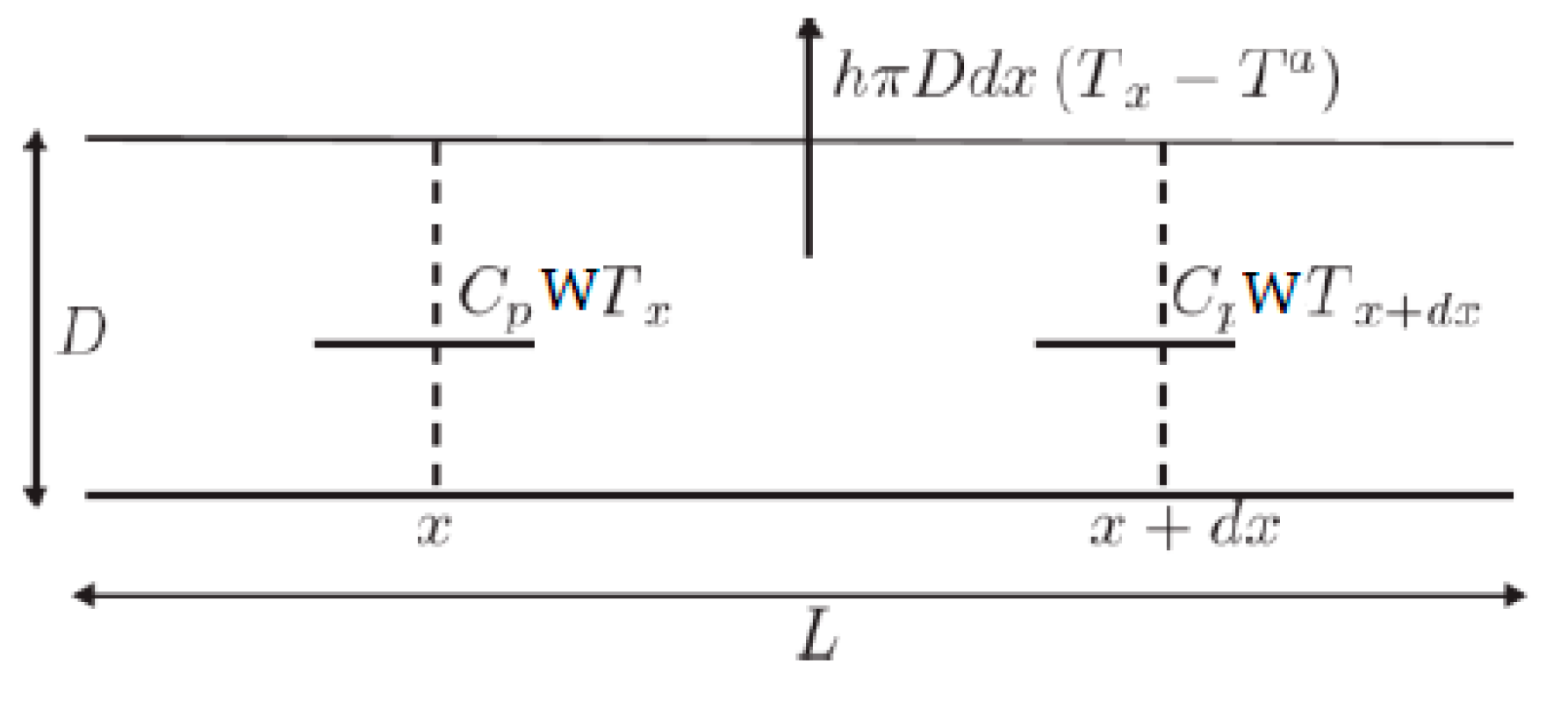
• an equation describing heat propagation along the pipeline, this equation can be written, by considering an infinitesimal volume along the pipeline (see Figure 5), as:

$$W{c}_p{\displaystyle \frac{dT}{dt}}=\lambda \left(T-T_{ext}\right)$$

(28)

where W is the mass flow rate, c_p is the specific heat, T the fluid temperature along the pipeline, T_ext the external temperature, λ = h A = h π D, being h the heat transfer coefficient, A the area of a section of the pipeline and D the diameter of the pipe.

By integrating equation (28) yields:

$$T_2-T_{ext}=exp\left({\displaystyle \frac{-\lambda L}{W{c}_p}}\right)\left(T_1-T_{ext}\right)$$

(29)

where T₁ and T₂ are the temperatures at the two extremes of the pipeline.

Heat loads are the elements of a heating system where heat is injected into and taken out of the system. Heat loads are generally modeled as heat exchangers. A basic model for a heat exchanger expresses the total injected heat power Δφ of a heat load as the change in the heat power between directly before and directly after the heat exchanger. Since a heat load is a connection between the supply and the return line of the heating system, the equation describing this process is:

$$\Delta \phi =c_{p}W\left(T^s-T^r\right)$$

(30)

where Δφ is the thermal power of the heat load, c_p is the specific heat, W the mass flow rate of the water circulating through the heat exchanger and T^r and T^s are respectively the temperatures of the supply and return lines of the heat network.

Further information on technical literature concerning the different approaches adopted for modelling heat networks and the relevant tools can be found in two extensive review papers ([41,42]).

3. Typical ME Approaches

The previous section dealt with different approaches to model single energy carriers (electricity, gas or, more in general, compressible fluids, heat). The interest there was to highlight pros and cons of different approaches useful for building up very large static ME models. This chapter introduces the most typical modelling approaches to be used for simulation and optimization of MES, including equations and factors describing the energy transformation between the different carriers.

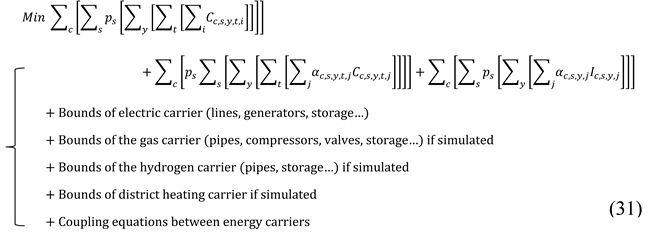
The optimization system (31), extension of the approach described in [43], provides the most general formulation for a ME optimization system for the co-optimization of the planning of all the considered energy carriers.

The target function minimizes total system costs (TOTEX) as a sum of total dispatching costs (OPEX, first two terms) and investment costs for new infrastructure (CAPEX, last term). The nested sums are referred to the following indices:

• c: energy carrier
• s: probabilistic scenario of RES production and load; $p_s$ is the probability associated to each single scenario
• y: time horizon considered for the planning problem (typically a few years or decades, e.g. [43] where three decades are considered: 2030, 2040, 2050)
• i: index enumerating each equipment in the system (e.g. electric lines): $C_{c,s,y,t,j}$ is the generic equipment item; ${\alpha }_{c,s,y,t,j}$ the integer variable associated to its investment.

If a sheer optimization of the dispatch (OPEX) is considered instead, all the parts of the objective function where the planning candidates are included must be omitted (these parts are easy to spot because multiplied by the investment integer variables α) as well as the summation over the planning time horizon (index y).

Finally, in case a load flow is what is sought for, the objective function is completely omitted and only the equations defining the set of constraint for all the carriers as well as the conversion equations between carriers should be considered.

The following sections will detail how the constraints equations must be written for each of the considered carriers. Three modelling representations will be considered in detail (energy hub, graph and self-consumption-based model). Then a further approach will be hinted at, which includes a joint planning of electricity and hydrogen networks, also contemplating the possibility that hydrogen is transported in lumped quantities by means of cylinder trucks. A synthetic presentation of other recent modelling representations will complete this overview.

Energy hub representation

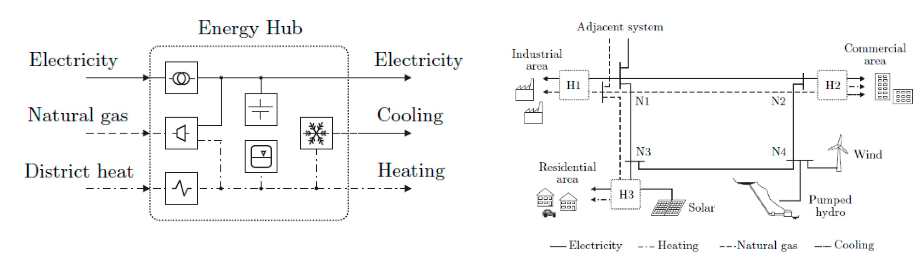
The Energy Hub (EH) representation was first introduced in [44]. Here, an EH is identified as a unit that provides energy conversion and storage of multiple energy carriers. Thus, the EH represents a generalization or extension of a network node of the electrical system. The whole energy supply infrastructure can be considered as a system of interconnected energy hubs (Figure 6).

Let’s consider a single converter device, which converts energy carrier α into carrier β. Input and output power flows are coupled through the following relationship:

$$L_{\mathsf{\beta }}=c_{\mathsf{\alpha }\mathsf{\beta }}{P}_{\mathsf{\alpha }}{L}_{\mathsf{\beta }}\le P_{\mathsf{\alpha }}0\le c_{\mathsf{\alpha }\mathsf{\beta }}\le 1$$

(32)

where P_α and L_β are the steady-state input and output power of the conversion process and c_αβ is a factor expressing the efficiency of the conversion.

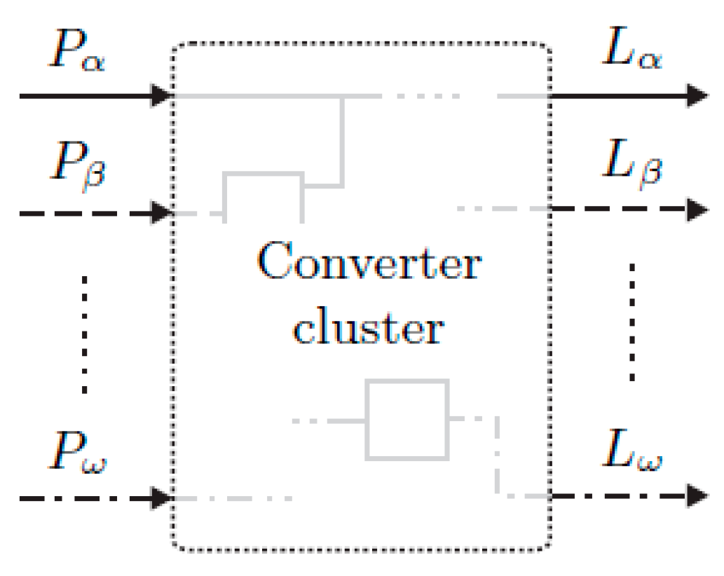
In case of a converter cluster (Figure 7) where multiple inputs are converted into multiple outputs either by a single device or by a combination of multiple converters., this can be represented analytically as:

$$\left[\begin{array}{c}{L}_{\alpha }\\ \dots \\ L_{\omega }\end{array}\right]=\left[\begin{array}{ccc}{c}_{\alpha \alpha }& \cdots & c_{\omega \alpha }\\ ⋮& \ddots & ⋮\\ c_{\alpha \omega }& \cdots & c_{\omega \omega }\end{array}\right]\left[\begin{array}{c}{P}_{\alpha }\\ \dots \\ P_{\omega }\end{array}\right]\mathrm{In}\mathrm{matrix}\mathrm{terms}:L=CP$$

(33)

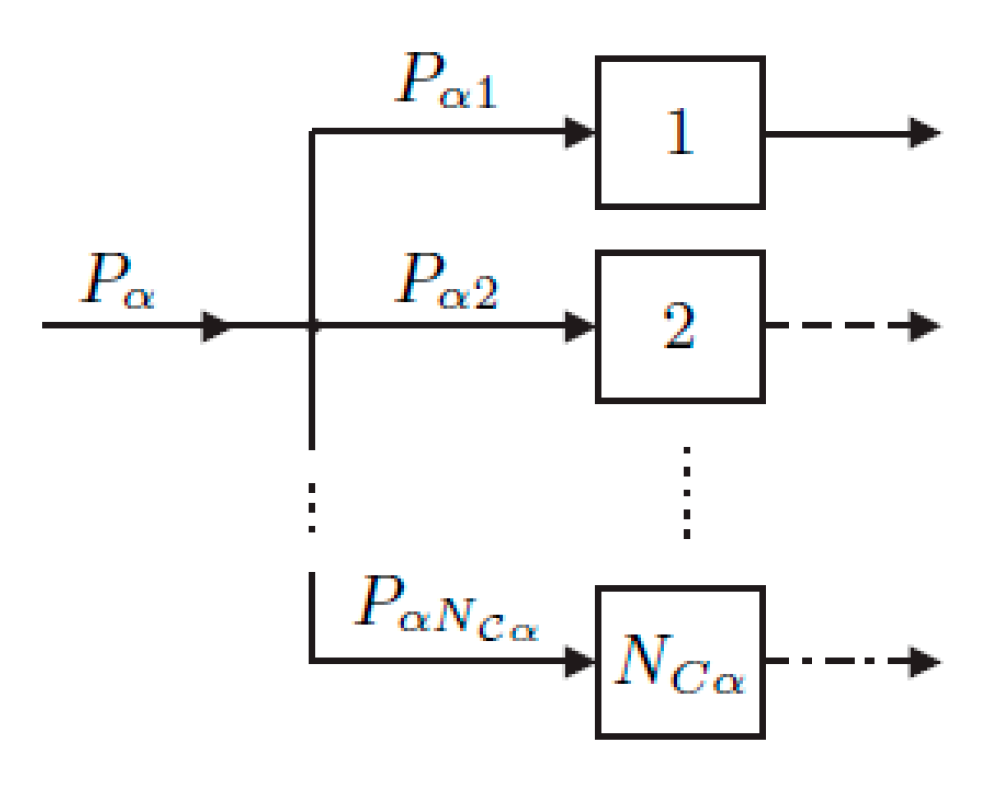
The total input of one energy carrier may be split up between several converters at input junctions (see Figure 8). For this, the so-called dispatch factors ν are introduced, as follows:

$$P_{\mathsf{\alpha }\mathrm{k}}={\nu }_{\mathsf{\alpha }\mathrm{k}}{P}_{\mathsf{\alpha }}0\le {\nu }_{\mathsf{\alpha }\mathrm{k}}\le 1{\displaystyle \sum }_k{\nu }_{\mathsf{\alpha }\mathrm{k}}=1$$

(34)

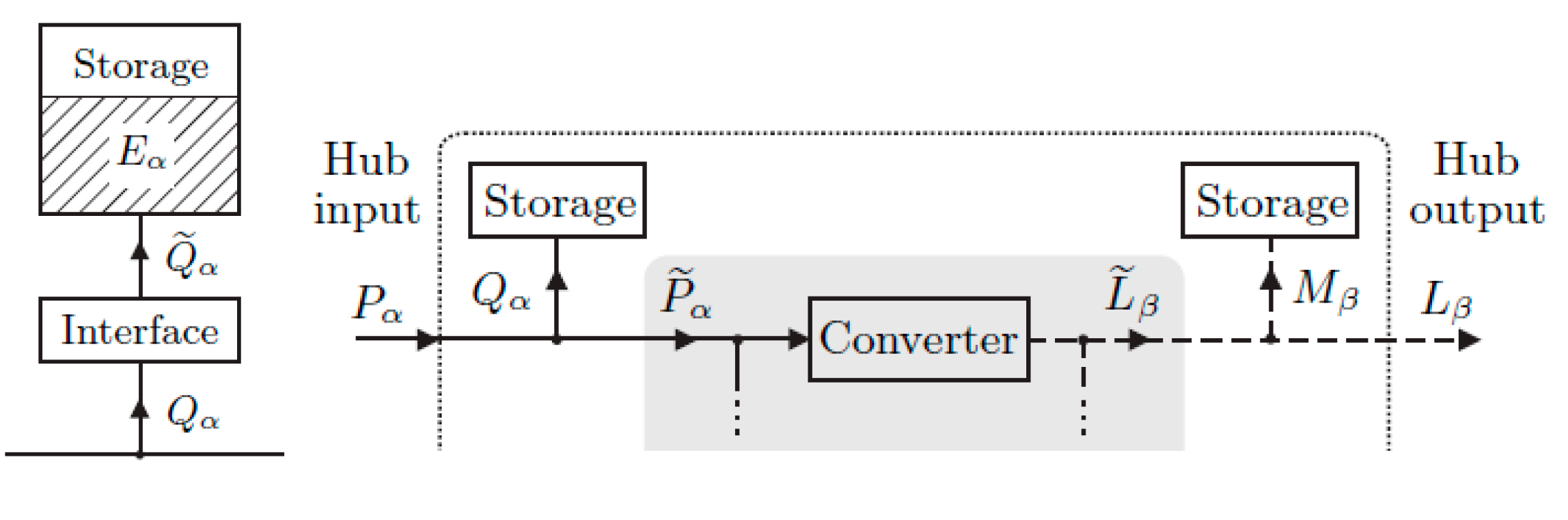
Storage units interfaces can be modeled as they were converter devices (Figure 9 left):

$$\widetilde{Q_{\alpha }}=e_{\alpha }{Q}_{\alpha }{e}_{\alpha }={e_{\alpha }}^{+} if Q_{\alpha }>0;1/{e_{\alpha }}^{-}else \widetilde{Q_{\alpha }}={\displaystyle \frac{d{E}_{\alpha }}{dt}} =\dot{E_{\alpha }}$$

(35)

where $\widetilde{Q_{\alpha }}$ and $Q_{\alpha }$ represent, respectively, the amount of energy actually stored, and the amount of energy fed for storage; ${e_{\alpha }}^{+}$and $1/{e_{\alpha }}^{-}$ represent the storage efficiency parameters for charge and discharge; $E_{\alpha }$ is the stored energy.

Considering the layout of Figure 9 right, storage units located upstream and downstream with respect to the converter can be represented as one only equivalent storage located downstream the energy conversion:

$${M_{\beta }}^{eq}=c_{\alpha \beta }{Q}_{\alpha }+M_{\beta }={\displaystyle \frac{c_{\alpha \beta }}{e_{\alpha }}}\dot{E_{\alpha }}+{\displaystyle \frac{1}{e_{\beta }}}\dot{E_{\beta }}$$

(36)

Generalizing:

$$\left[\begin{array}{c}{M}_{\alpha }^{eq}\\ \dots \\ M_{\omega }^{eq}\end{array}\right]=\left[\begin{array}{ccc}{s}_{\alpha \alpha }& \cdots & s_{\omega \alpha }\\ ⋮& \ddots & ⋮\\ s_{\alpha \omega }& \cdots & s_{\omega \omega }\end{array}\right]\left[\begin{array}{c}\dot{E_{\alpha }}\\ \dots \\ \dot{E_{\omega }}\end{array}\right]\mathrm{In}\mathrm{matrix}\mathrm{terms}\text{:} M^{eq}=S\dot{E}$$

(37)

Putting together (33) and (37):

$$L=CP-S\dot{E}=\left[\begin{array}{cc}C& -S\end{array}\right]\left[\begin{array}{c}P\\ \dot{E}\end{array}\right]$$

(38)

EHs are interconnected (Figure 10) through branches. Each branch is characterized by one or more components that are modelled according to the modalities described in chapter 2. The steady state of the overall system is described by a set of nodal balances and line equations (see also graph notation introduced in the subsequent section), which, generally, creates a system of nonlinear equations. EH input and output power contributions are included into such system as nodal injections.

Graph representation

Dissertation [5] presents a graph-based ([45]) framework for load-flow and optimization analysis of MES that consist of gas, electricity and heat. The overall framework is based on interconnecting single carrier networks through heterogeneous coupling nodes and homogeneous dummy links, to form one connected multi-carrier network.

Load flow equations consist of conservation equations written in a consistent way for all carriers according to the following two principles:

• first law: conservation of mass or energy for each node,
• second law: sum of potential differences over each loop is zero.

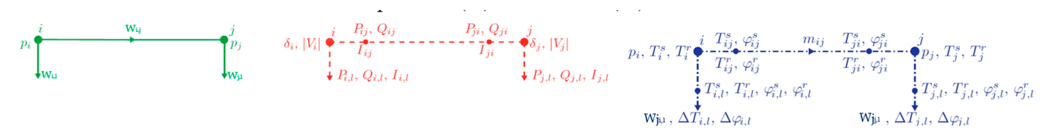
The graph representation for each carrier is schematized in Figure 11:

• green color for gas networks – variables: pressures (p) and mass flow rates (W),
• red color for electricity networks – variables: active powers (P), reactive powers (Q), voltages (V), angles (δ), currents (I),
• blue color for heat networks (the return line is not explicitly represented) – variables: pressures (p), thermal flows (φ), supply temperature (T^s) return temperature (T^r), water flows (W).

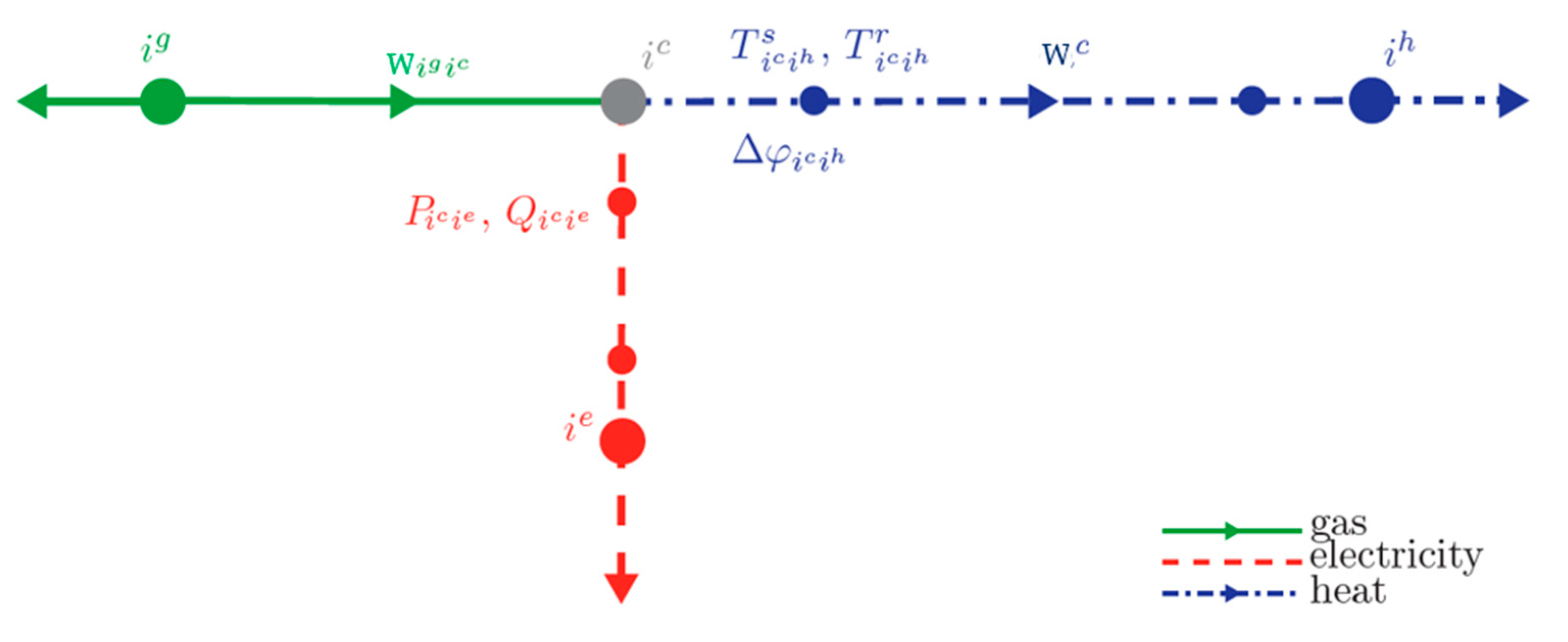
Single carriers are coupled by introducing fictitious coupling nodes (Figure 12). In every coupling node (i.e. energy conversion node), one or more coupling equations (i.e. energy conversion equations) hold. No variables are associated with a coupling node, because it does not belong to any of the single carrier networks. Therefore, links representing physical components cannot be connected to a coupling node. For instance, a link representing a gas pipe cannot be connected, since the flow model associated with the link requires both start and end node to have a nodal pressure p. Therefore, a dummy link is introduced to couple a coupling node to any other single carrier node. Dummy links do not represent any physical component: they merely show a connection between nodes. If a dummy link connects a coupling node and a single carrier node, the dummy link is of the same carrier as the single carrier node. As such, it has the same variables associated with it as any other link of that carrier. These variables are shown in figure at the side of the coupling node only. Although dummy links do not represent a physical component, they can be seen as lossless pipes or lines, conserving electrical energy across the line.

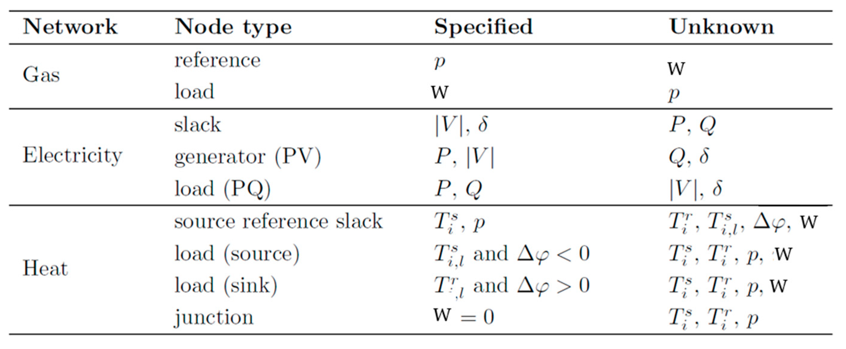
Provided energy injections and withdrawals are known for the whole ME system, a load flow analysis determines the flow of energy for each carrier. Typically, single carrier networks have more variables than equations. Therefore, some variables are assumed as known. Usually, border conditions are placed on a (terminal) node, usually called slack node, or on its terminal link. A node type is assigned to every node based on the variables that are locally (un)known (Table 3).

In a multi carrier system, a carrier coupling model introduces more unknowns than equations as well. Additional equations or boundary conditions are needed for the total system to be solvable. A possible choice is that some or all the energy flows to or from the couplings are assumed known as additional border conditions. However, this decouples the integrated system into a set of separate single-carrier parts, so that the flexibility provided by coupling energy systems is not fully used. Therefore, [5] assumes all coupling (energy) flows unknown and the additionally required border conditions are imposed elsewhere in the single-carrier parts. However, this must be done carefully, since not all combinations of load flow equations and border conditions for such integrated energy systems (consisting of gas, electricity, and heat) lead to well-posed problems.

Starting from the full set of conservation equations, written for nodes and loops of the ME graph, the mathematical system that solves the load flow problem can be easily put in matrix form (see [5]). Otherwise in the case of a planning or dispatch problem, an optimization problem should be solved, having the same load flow equations as problem constraints.

Self-consumption-based representation

Report [46] illustrates an interesting model aimed at optimizing the dispatch of MES. Here, we limit ourselves to describe the overall model setting, leaving the details for a detailed reading of the report.

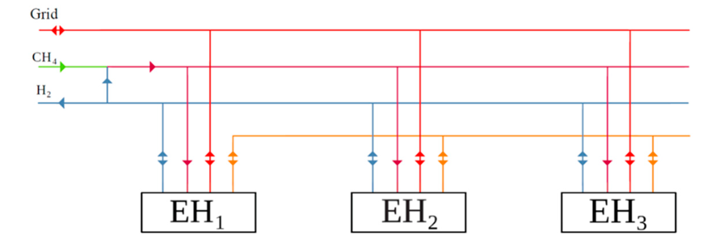
As shown in Figure 13, the multi-vector system described here is composed by several EHs connected:

• to the electric vector (in red), which can both buy and sell electricity,
• to the thermal vector (in orange) with which the EHs can exchange heat,
• to the hydrogen vector (in blue), which can be exchanged between the EHs,
• to the gas network (in green), where natural gas is purchased; natural gas can be used in its pure form or mixed with hydrogen (mixture, in magenta) potentially up to 20% to serve the EHs.

The main modelling hypothesis is that each EH works following a self-consumption priority philosophy, i.e. first satisfying its own energy demand, and then eventually reselling the surplus produced. Therefore, the developed algorithm is based on two separate mathematical models:

• the first model focuses on the single EH,
• the second model describes the multi-vector system, which is represented as a set of EHs, connected to each other through the three energy vectors.

First, the functioning of each EH is optimized separately, in order to incentivize self-consumption as much as possible, and then the residual flows are optimized by incentivizing the exchange between EH, thus simulating a local market.

The first optimization minimizes system costs over the entire considered time period, more precisely the sum of production costs, purchase costs from the network and revenues from sales to the network, adopting the following constraints:

• limiting the values ​​of the variables relating to generation and storage to a range between a minimum and a maximum value,
• satisfying the balances of electricity, heat and gas of the network for each time period,
• calculating the amount of energy stored in the storage systems for each instant (minimum storage at time t=0),
• determining the amounts of energy produced by each type of technology at any given moment,
• limiting the operating region for the cogeneration plant,
• imposing that the gas storage system cannot both supply and store gas at the same time (a few binary variables are introduced),
• and imposing similarly (binary variables):

  ○

  that the battery cannot supply and store electricity at the same time,

  ○

  that the heat storage system cannot supply and store heat at the same time,

  ○

  that the EH cannot sell and buy heat at the same time,

  ○

  that the EH cannot sell and buy gas at the same time.

The second optimization (see conceptual scheme in Figure 14) optimizes the residual flows of the three energy vectors by incentivizing the exchange between EHs. The basic idea is to consider the multi-vector system as a graph. Each EH can be identified by a node i, while each transmission line between nodes i and j can be described by an arc (i,j). Since the system is composed of three different energy vectors, there are actually three distinct graphs, one for each energy vector. For each one of the three graphs, a transmission cost is defined between each couple of EHs.

Furthermore, for each node i at each instant of time t, the residual flows of the three energy vectors are given as input data as a result of the previous optimization step.

The objective function minimizes the transmission costs of the multi-vector system over the entire considered time period T. These costs are calculated on the basis of the flows transmitted in each period between the nodes. The optimization constraints are:

• flow balances of the electric vector,
• flow balances of the heat vector,
• flow balances of the gas vector,
• limitation between 0 and max of energy flows between EHs of the three vectors,
• Weymouth equation (12) to describe gas flows, linearized according to [34].

The rigid division between the two optimizations introduces a sub-optimum in the optimization process and the underlying hypothesis of self-consumption prioritization is not rigorously true. Additionally, the flow model applied to the second optimization stage as depicted in Figure 14 doesn’t strictly adhere to the laws of physics (yet being still acceptable for a local market in a small geographical extension). Nonetheless, this approach is interesting because it shows an attempt to define a rationale for setting up a decoupling of the solution mechanism to help retaining numerical tractability of big ME models.

Joint planning of electricity and hydrogen transportation

In the frame of the present decarbonization policies implemented in Europe and elsewhere, hydrogen is possibly the most promising vector to be utilized in the future for heavy transport as well as the so-called hard-to-abate industry sectors [2]. Hydrogen produced by electrolysers (“green hydrogen”) can be sent to the utilizers through a dedicated transport infrastructure. The costs to create such infrastructure can be reduced by reutilizing (“repurposing”) part of the existing gas pipelines. However, until hydrogen demand, which is expected to gradually increase, will not attain a given amount economically justifying the buildup of a dedicated infrastructure, the most convenient way to transport will remain to use gas cylinder trucks. We can also think of an intermediate scenario, in which demand will start to be satisfied with hydrogen coming from a dedicated network, but part will still be supplied with trucks. 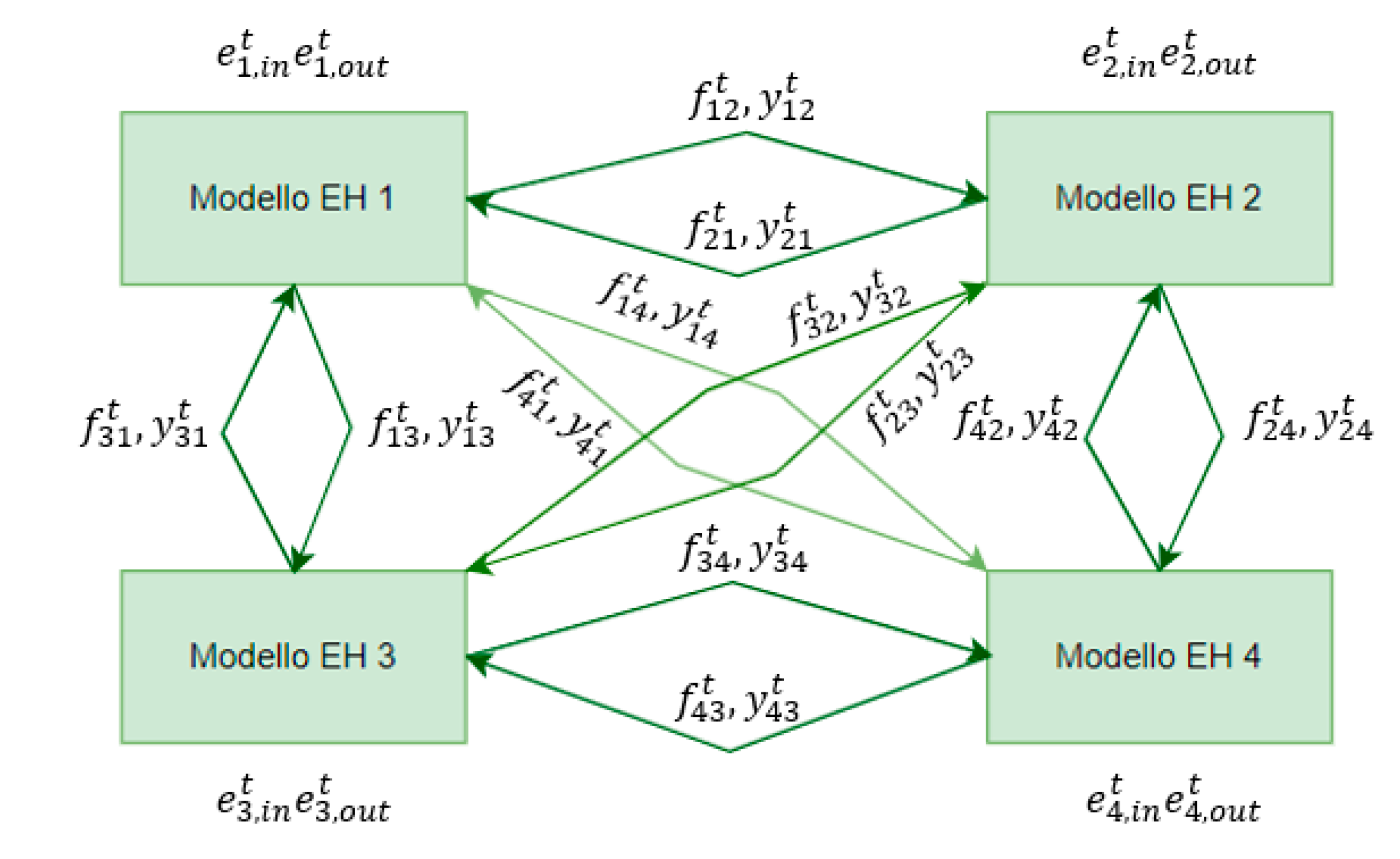This is the situation the modelling approach described in [47] refers to.

The paper proposes a joint grid planning approach for both power and hydrogen grids which coordinately optimizes investments and operation on the two networks. Both a deterministic optimization approach and a robust planning under uncertainty [20] are tested. Three hydrogen modelling aspects are specifically addressed and combined: truck routing, pipeline transportation and storage. We will provide a conceptual introduction to the approach, leaving the in-depth analysis to a careful reading of the paper.

Regarding the truck transportation network (see Figure 15), the hydrogen quantity in charged and empty trucks in each zone changes according to leaving and arriving schedules as well as charging and discharging behaviors of trucks. The quantity e^tru_k,z,s,d represents the hydrogen quantity in charged trucks with transportation technology k in zone z at the end of day d in scenario s. Travel time delay is taken into account. If charged trucks with q^tru_k,m,n,s,d hydrogen quantity leave at the end of day d from zone m to zone n, when accounting a time delay of T_k,m,n days, the same quantity of hydrogen arrives in zone n at the beginning of day d+T_k,m,n. Empty trucks can also be transported between any two zones and the transportation of empty capacity can be modelled too. The total amount of full and empty truck capacity in all zones during day d can be calculated as the total amount staying in each zone at the end of the previous day plus the amount just arrived at the beginning of day d.

To preserve numerical tractability, a simplified linear model is adopted for hydrogen pipeline networks. Linepack storage dynamics of each pipeline is represented too.

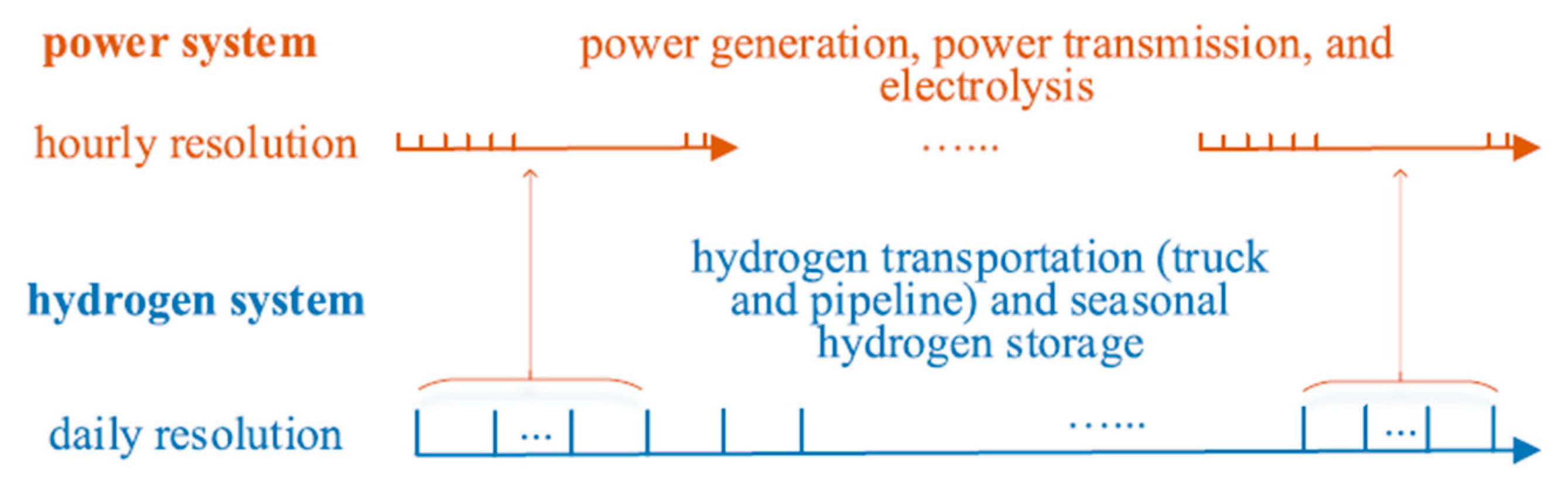
Hydrogen and electric storage are fully modelled. Conventional electric storage, such as pumped storage and battery storage, are considered as operated in daily or weekly cycles. In each storage cycle, time periods are considered as sequential.

As both power and hydrogen systems are incorporated in the proposed planning approach, system components with distinctive physical characteristics need to be modeled in different time scales. In hydrogen systems, hydrogen storage usually has seasonal cycles, and truck transportation takes a few days to travel between two zones. In power systems, steady-state models in planning problems usually have an hourly resolution, as electric demand and renewable energy output fluctuate in a relatively short time frame. Thus, different resolutions are applied for resources with different timescales in our optimization, as shown in Figure 16: hydrogen system components are modeled in daily resolution while power system components are modeled in hourly resolution.

The objective function is the sum of the investment and operation cost for truck and pipeline, hydrogen transportation, hydrogen production, hydrogen storage, as well as electric power generation and transmission. Among the optimization constraints:

• for hydrogen:

  ○

  zonal hydrogen quantity balance constraints,

  ○

  hydrogen production limits for the electrolyzers

• for the electric system:

  ○

  electric power balance for each bus,

  ○

  limits for renewable power output,

  ○

  power output and ramp rate for conventional generators,

  ○

  branch flow for existing transmission lines (direct current approach),

  ○

  flow-angle relations and flow limits for candidate lines.

Other approaches

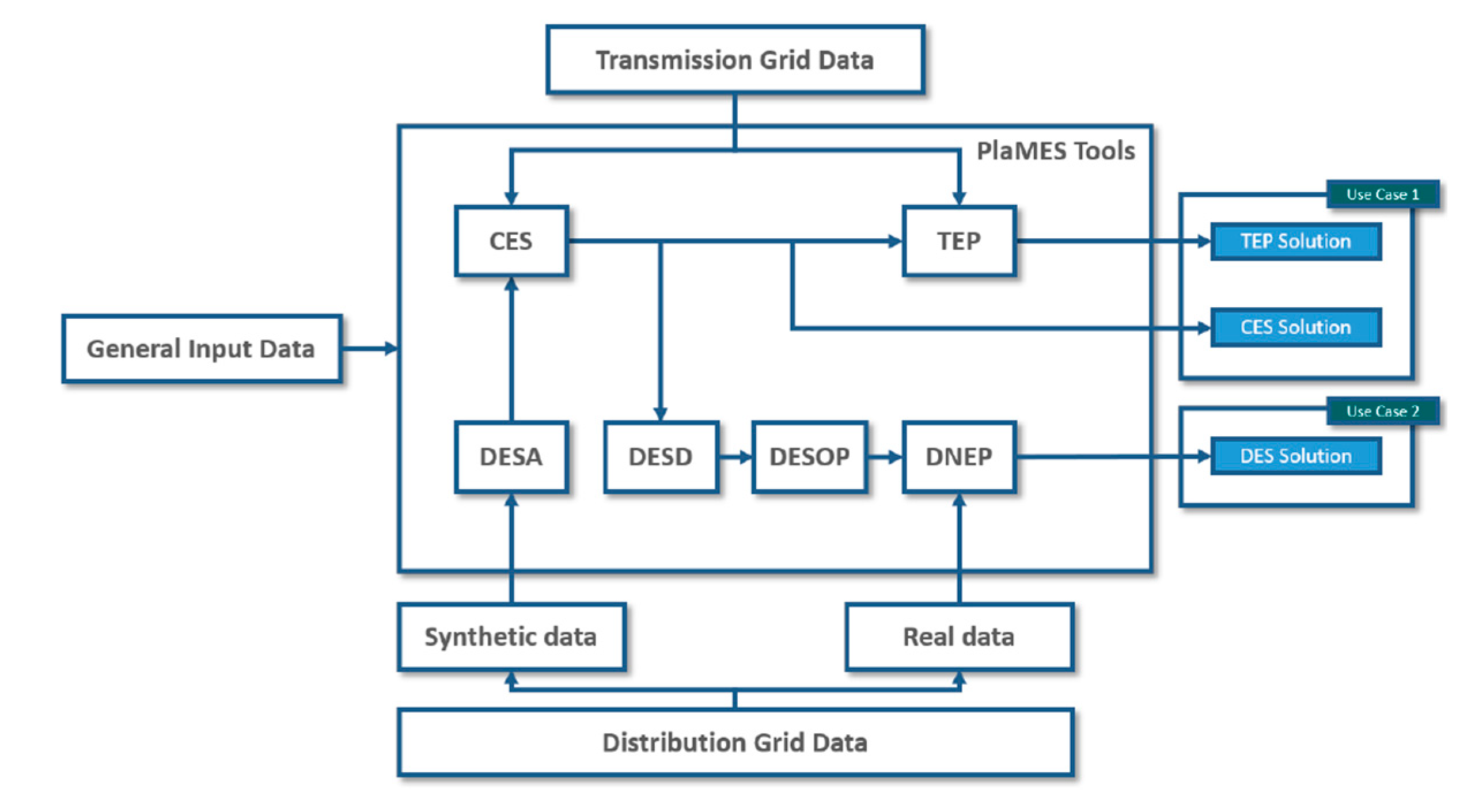
The PlaMES research project ([48]) aims at developing an integrated planning tool for MES at a European scale. The PlaMES model considers the coupling of different energy sectors (electricity, heat, mobility and gas) and calculates the cost-optimal energy mix for the future European energy system (e. g. up to 2050) compliant with the climate goals. These modeling requirements lead to write a large mixed-integer (non-linear) optimization problem. Besides generation and storage systems, also transmission and distribution grids are considered in the planning and operation stage in an integrated way. The complete modelling approach is described in deliverable D2.2 ([49]). It contemplates the use of six tools (see Figure 17) carrying out a single stage optimization procedure each. These tools can also be used separately, but the procedure foresees their coordinated usage to cope with the complete planning procedure. The focus is on the electricity carrier, the other ones being modeled only for their interactions with the electricity carrier.

The six tools perform the following tasks:

• DESA (Decentral Energy System Aggregation) derives costs for each decentral network area by performing a distribution grid expansion planning for various supply tasks depending on the integration of technologies to the respective area. The result of this model can then be used in central planning.
• In a fully linearized approach, CES plans the Central Energy System, taking data from DESA and the transmission grid into account.
• The result of the CES will then be given to the TEP (Transmission Expansion Planning) module, which focuses on a detailed expansion planning approach analyzing different expansion technologies and congestion management interventions.
• DESD (Decentral Energy System Disaggregation) undertakes the placing of renewable energy sources and other assets, that have centrally been planned in CES for a Decentral Energy System (DES).
• The operation of a DES can be performed by the DESOP (Decentral Energy System Operational Planning) module and can be enriched by information from CES.
• The DNEP (Distribution Network Expansion Planning) module implements an optimization approach to calculate the distribution network expansion planning.

As shown above, the PlaMES approach is strongly fragmented in sub tasks. If this helps, on one side, to tackle high-dimensionality problems reducing them to tractable numerical optimizations, on the other side there is a high risk to calculate a sub-optimal solution. Additionally, detailed planning approaches implemented in the last steps might suffer the consequences of important approximations taken to calculate the former steps, which provide the latter with input data.

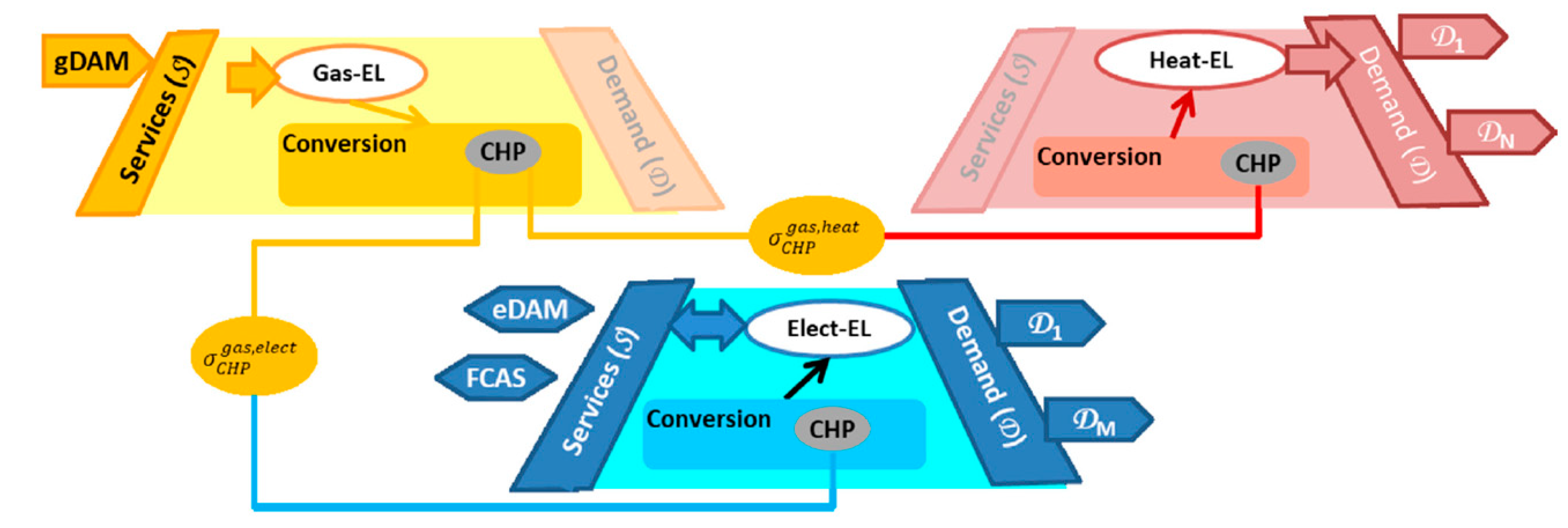
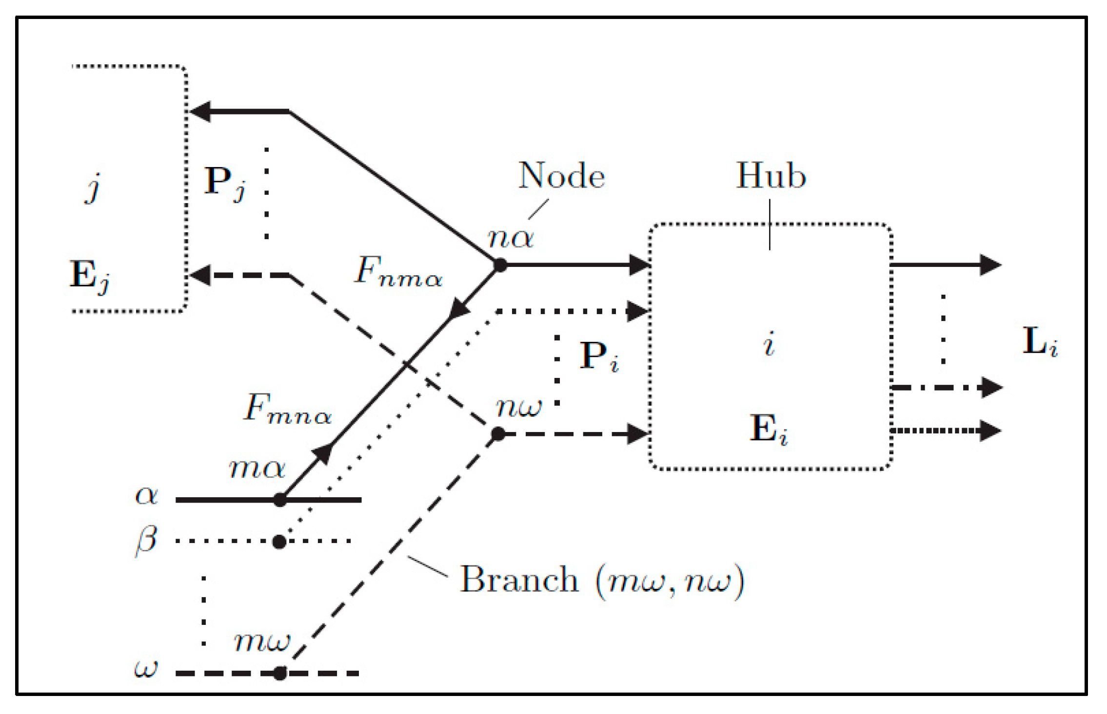
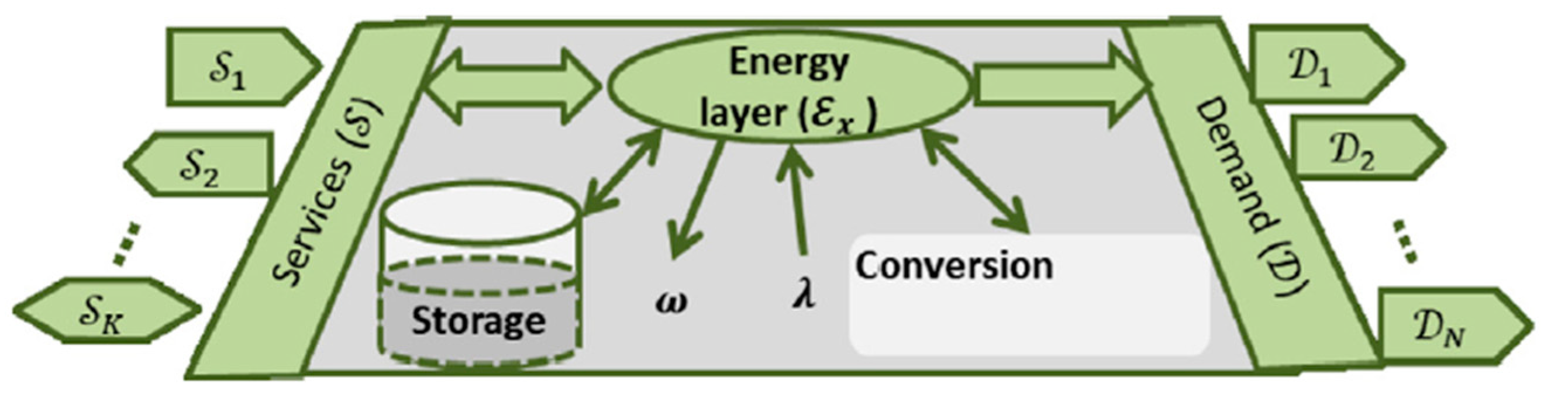
An interesting approach on optimizing participation of MES to energy and ancillary services markets is adopted by the MAGNITUDE project ([50]), which aims to develop business and market mechanisms as well as supporting coordination tools to provide flexibility to the European electricity system, by increasing and optimizing synergies between electricity, gas and heat systems. As described in ([51]), the MAGNITUDE project develops a novel modelling framework and an associated optimization methodology for short-term operational planning to deploy MES flexibility, with application to district energy systems and participation in energy and Frequency Control Ancillary Services (FCAS). The approach is based on the concept of ME lattice, which models MES by splitting them into several energy layers (see Figure 18), each one associated with a specific energy carrier. There can be multiple services associated with an energy carrier. Each service can be for “import”, “export”, or “dual-mode”: the import services require an increase in the import (or decrease in the export) of an energy carrier, export services require increase in the export (or decrease in the import) of an energy carrier, while dual-mode may require both directions of energy flows. Figure 19 provides a simple example of application referred to a Combined Heat and Power plant (CHP, [52]).

The MAGNITUDE project defines different kinds of flexibility to be provided by MES and associates each of them to the relevant services it can provide (see Figure 20):

• Physical: maximum flexibility available on the energy vector and is quantified by its operational range.
• Operational: modulation capability for an energy carrier that MES can provide with respect to (starting from) a given operating point. The operational flexibility of a device is divided into two components: upward and downward.
• Carrier-balancing: operational flexibility for an energy carrier, reduced by the constraints imposed by the other energy carriers through conversion nodes. The energy vectors of MES are coupled and cannot be viewed independently: the operational flexibility available to an energy vector is also impacted by the constraints of other energy vectors.
• Market-product: carrier-balancing flexibility subject to market product constraints, e.g., maximum allowed activation time, minimum service duration, which further limit the flexibility that can be provided by a cluster of resources.
• Economic: flexibility that the MES operator can offer at a given cost for a specific service and accounting for MES economic objectives (to be optimized). A device will only participate in a given service if the revenues are greater than the cost of delivering that service.
• Market: economic flexibility cleared and accepted by the market given the market requirements and other offers.

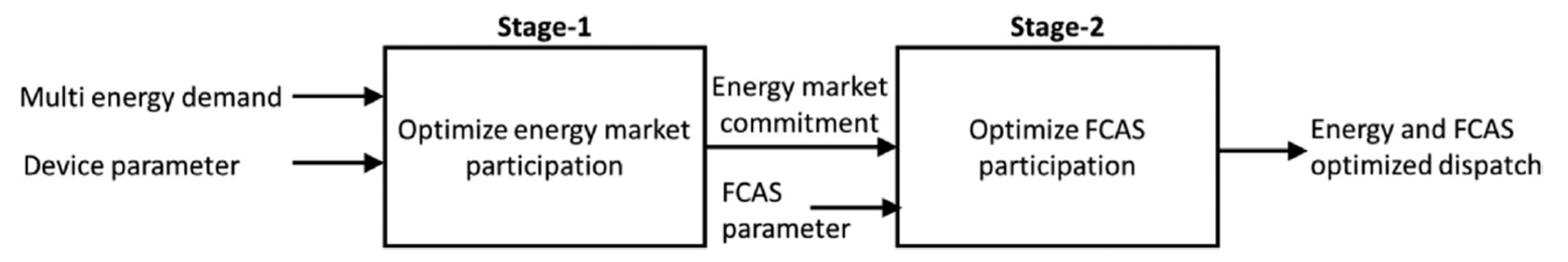
The energy market is modeled as a simplification of the standard market design implemented in many European countries and elsewhere, as schematized as in Figure 21. Stage 1 optimizes the participation of the MES in various energy markets while fulfilling multi-carrier demand(s) requirements. The decision variables obtained from the first stage of the methodology are then provided as input parameters to the second stage, which optimizes FCAS participation. The outcome of the second stage is the optimal scheduling of the resources in the ancillary service market.

Two further European still on-going research projects, iDesignRES ([53]) and MOPO ([54]) are dedicating their efforts to create advanced tools using multi-energy modelling.

Finally, it is worth mentioning that the Los Alamos National Laboratory’s Advanced Network Science Initiative ANSI ([55]) has recently developed a few interesting open access and open source libraries for modeling infrastructure networks ([56]). In particular, the library GasPowerModels.jl (using the Julia programming language [24]) is dedicated to the joint optimization of power and natural gas transmission networks.

4. Conclusions

The above pages of this paper have introduced some of the most typical approaches present in today’s technical literature to describe static models of MES, either resulting in equation systems utilized to solve load flow problems or in optimization systems to calculate optimal dispatch or grid planning or market allocation. ME problems have the characteristic to require a very large number of variables to describe all the implemented carriers with a reasonable level of detail. Often, integer variables are implied as well (e.g. for optimal planning investment problems), making the optimization problem a MILP problem, solved by using branch-and-bound techniques, possibly simplified by adopting some decomposition technique. The most typical one is Benders’ decomposition, which proves particularly convenient for implementations based on parallel computing platforms and programming languages allowing to distribute computation over parallel processors, as it is the case for the most recent high-level languages, like MATLAB and Julia. In this frame, getting a linear or linearized modelling for the represented MES components is of paramount importance to ensure system convexity and allow using fast linear systems solving techniques.

The first part of this paper was devoted to analyzing separately the components of each single carrier: electric, compressible fluids (gas/hydrogen) and heat networks. While the linearization brought by the direct current approximation is often acceptable for static studies of electric networks, most components of gas and heat networks (long elements, compressors, regulation valves) have non-linear mathematical descriptions. Yet, linearization techniques do exist, which should be utilized whenever this is acceptable. The required modeling approach strongly depends on the type of study to be carried out: grid planning, operational optimization, optimization of the services that the MES can provide, etc. It must also be noted that very few literature articles deal with modeling for ME planning. Grid planning has strong peculiarities (it might require fewer modeling details on the individual components, but the number of variables is much higher, having to simulate much longer time horizons and including extra variables related to investments).

The second part of the paper was devoted to describing approaches to the joint representation of the different MES carriers. Energy hubs and graphs, two classic modelling tools for MES, are first introduced. Then, other approaches are presented, including an interesting one allowing to model also cylinder truck-transported hydrogen.

In conclusion, it must be admitted that matching a numerically tractable technique to the solution of very large MES (like the most general one described by (31)) is still a daunting task and a field of research: numerical techniques are gradually adapted to the steadily increasing performances of computer hardware and software. On this regard, recently, the introduction of cloud computing ([57]) has brought new possible horizons.