
Submitted:
26 February 2025
Posted:
27 February 2025
You are already at the latest version
Abstract
This study explores the application of wireless wearable devices within the emerging domain of biomechanical feedback systems for sports and rehabilitation. A critical aspect of these systems is the need for real-time operation, where wearable devices must execute multiple processes concurrently while ensuring specific tasks are performed within precise time constraints. To address this challenge, we developed a specialized, lightweight periodic scheduler for microcontrollers. Extensive testing under various conditions demonstrated that sensor sampling frequencies of 650 Hz and 1750 Hz are achievable when utilizing 1 and 26 sensor samples per packet, respectively. Receiver delays were observed to be a few milliseconds or more, depending on the application scenario. These findings offer practical guidelines for developers and practitioners working with real-time biomechanical feedback systems. By optimizing sensor sampling frequencies and packet configurations, our approach enables more responsive and accurate feedback for athletes and patients, improving the reliability of motion analysis, rehabilitation monitoring, and training assessments. Additionally, we outline the limitations of such systems in terms of transmission delays and jitter, providing insights into their feasibility for different real-world applications.
Keywords:
wearable devices
; periodic scheduler
; sensors
; IMU
; microcontroller
; real-time biofeedback
; sport
; physical rehabilitation
1. Introduction
Advancements in Information and Communication Technology (ICT) have significantly contributed to various research fields, thereby enhancing overall quality of life. One such field is development of biomechanical feedback systems for sports and rehabilitation, which we address in this paper. These systems aim to acquire, monitor, analyse, assess, and improve human movement patterns in real time. While initially developed for sports performance enhancement, biomechanical feedback has also found applications in physical rehabilitation, helping patients regain mobility and correct movement patterns [1-2].
A crucial aspect of biomechanical feedback systems is the timing of feedback delivery [1], which determines when corrective information is provided to the user. Feedback can be terminal (delivered after task completion), concurrent (provided in real time during the movement), or cyclic (offered immediately after completing a repeating motion cycle). Wearable devices play a key role in enabling real-time feedback, as they allow unobtrusive monitoring and wireless communication with processing units. These devices are worn on the body as accessories, attachments, or implants and encompass a broad spectrum—from smart devices like smartphones and smartwatches to small accessories such as smart eyewear, and specialized sensor devices or intelligent sports equipment [3]. Comprehensive overviews of wearable devices and their associated challenges are provided in [4-5], while their technical challenges and limitations are explored in [6-7].
When evaluating wearable sensor devices for RTBF, our focus was primarily on kinematic sensors, such as inertial measurement units (IMUs) [13]. They are widely used in wearable technologies for performance enhancement and risk assessment in various fields, including sports, industry [14], and rehabilitation [15]. IMUs employ gyroscopes and accelerometers to capture body motion, and are sometimes used to supplement marker-based optical systems for monitoring high-speed motion in sports [16]. Other types of sensors, such as piezoelectric [17] or triboelectric [18], are available for measuring human activities, body processes and states, but they do not fall into the scope of this work.
Real-time biomechanical feedback (RTBF) applications for analysing human motion require strict time guarantees, especially when high sampling frequencies are required, often exceeding 100 or 200 Hz [10]. We have previously conducted a study to determine the most commonly used approaches in RTBF applications [8] and were surprised to find that none of the articles we reviewed explicitly discussed specific software mechanisms for handling real-time constraints. Even when timing requirements were mentioned, they were often vague or not directly related to software implementation. For instance, in [19], the authors stated that "the microcontroller continuously calculates the current position," but did not provide specific details about the timing constraints. In another study, [20], the authors reported choosing a time window of 12 seconds and a sampling frequency of 64 Hz for EEG signals, but did not specify any timing requirements for the accelerometer readings, which they described as "instantaneous measurements." The most stringent timing requirements we found were in [16], where a capture rate of 1000 Hz was required, but even in this article, no details were provided on how the system ensured precise timing and synchronization.
Wearable sensor devices for RTBF systems must execute multiple processes in parallel, including: acquiring sensor data at uniform time intervals, formatting and assembling data packets, and transmitting sensor data wirelessly while maintaining minimal latency. Ensuring precise timing and synchronization across these processes presents a technical challenge, particularly given the limited computational resources of battery-powered microcontrollers. Several Real-Time Operating System (RTOS) solutions are available for real-time embedded applications, including FreeRTOS, ChibiOS, and NuttX. These systems provide features like pre-emptive multitasking, priority-based scheduling, and inter-task communication, making them suitable for general-purpose real-time applications. However, for RTBF applications, these features introduce unnecessary overhead, making them less suitable for resource-constrained wearable devices.
To address these challenges, we developed a lightweight periodic scheduler tailored to the specific needs of real-time biomechanical feedback applications. Unlike full RTOS solutions, which provide complex task management features, our scheduler follows a cooperative round-robin execution model, ensuring minimal overhead and precise timing control. This design allows us to achieve:
- Minimal overhead - It is lean and efficient, avoiding excessive memory usage or processing time that could interfere with other processes.
- Task-specific design - It performs only the essential functions required for our wireless sensor device, without unnecessary complexity.
- Configurability - It is adaptable to various application scenarios, such as streaming, logging, or event detection.
- Cost-effective and energy-efficient design - Since wireless systems often operate on battery power, energy efficiency is important for prolonged use. However, considering that our device is intended for shorter operational intervals in environments with accessible charging options, cost efficiency also plays a key role. The scheduler should therefore maintain a balance between low power consumption and affordability, ensuring an optimal trade-off between performance, energy usage, and price.
The primary research question addressed in this study is: What is the maximum sensor sampling frequency that can be supported by a given wearable device in streaming mode? In answering the question, the following contributions were identified: (a) development and implementation of a lightweight periodic scheduler tailored to the specific needs of real-time biomechanical feedback applications and adaptable for other real-time data acquisition tasks, (b) a wearable RTBF system with flexible sensor sample streaming capabilities covering a range of possible needs in sports and rehabilitation, (c) determination of the upper limit of the sampling frequency for the specific hardware we used with different formats and numbers of samples in a package.
2. Materials and Methods
In order to meet the requirements of being lightweight and autonomous, we chose the Adafruit Feather M0 board, which features an ATSAMD21 microcontroller and ATWINC1500 network controller, as a base of our system. The compact size and weight of the board make it unobtrusive to the wearer's movement, and it can be mounted discreetly.
2.1. System Architecture and Implementation
To acquire comprehensive motion data, we utilized the MinIMU-9 v5 board from Pololu [13], which integrates two sensor chips manufactured by STMicroelectronics: the LIS3MDL magnetometer [11] and the LSM6DS33 accelerometer and gyroscope [12]. Together, these sensors provide measurements along three axes each, totalling nine degrees of freedom essential for detailed analysis of human movement. The sensor assembly was connected to the Adafruit Feather M0 microcontroller board via the I²C communication interface, as shown in Figure 1. For our initial testing phase, we employed the Arduino library supplied by Pololu to configure the sensors and retrieve raw data outputs.
We utilized Pololu's Arduino library to maintain compatibility with the Arduino environment, but for effective debugging, a more advanced Integrated Development Environment (such as a CMake project in Visual Studio Code using the Cortex-Debug extension) is necessary.
In Figure 2, we present three examples of system implementations that we use in various biofeedback applications developed in our laboratory [21]. These are prototypes that will later be built into different enclosures and used as 9 DoF wearable devices with wireless communication. These are some of the devices used in the tests and measurements presented in later sections of this article.
2.2. Scheduler Implementation
To achieve uniformly spaced sensor readings, we developed a custom cooperative periodic scheduler without task prioritization. This scheduler employs a round-robin execution model capable of handling a variable number of finite tasks, each of which must be completed within a predefined time slice. By utilizing a modular and transparent software architecture, our system prevents race conditions and CPU starvation through cooperative task scheduling without priorities. This implementation leverages a single timer interrupt, as illustrated in Figure 3. As shown in the figure, the system masks native Arduino interrupts during the execution of the timer interrupt and permits them only between the scheduled tasks.
By imposing stringent constraints on the tasks supported by our system, we were able to simplify it to its bare minimum. As shown in Figure 3, tasks are executed in a strict round-robin fashion, and it is the user's responsibility to ensure that each task completes before the next timer interrupt occurs. Upon each interrupt, the scheduler simply retrieves the address of the next task to be executed and runs it. This approach imposes only about 3 μs of overhead, which is significantly lower than the overhead imposed by any of the RTOS solutions presented in the previous section.
As a direct consequence of the aforementioned simplification and overhead reduction, we were able to utilize a less powerful, energy-efficient microcontroller without compromising real-time performance. This design choice inherently contributes to lower power consumption, as the selected processor operates with reduced computational demands1. Additionally, the scheduler itself occupies less than 1 kB of the 256 kB of available flash memory, leaving sufficient capacity for the remaining program code and future extensions. The SRAM utilization is similarly low, as this memory primarily serves as a buffer for sensor readings prior to transmission via the Wi-Fi interface. Since data is transmitted continuously with minimal buffering, the required SRAM remains well below 1 kB.
Due to the deterministic nature of task execution, no conflicts or unexpected task delays were observed under normal operation, as long as each task adhered to its allocated time slice. The primary challenge arises in high-load scenarios where a transmitted packet is not successfully received due to network conditions or interference. However, this is not a limitation of the scheduler itself; rather, it is handled at the communication protocol level, where the system simply requests a packet resend as needed. This ensures that data transmission remains reliable without disrupting the strict timing requirements of the real-time biofeedback process.
2.3. Preliminary Tests
Preliminary tests indicate that the minimum feasible time slice is constrained by the duration of a single raw data reading, which is approximately 330 μs for one nine-degrees-of-freedom data sample. Assuming no additional tasks are executed, the maximum achievable sampling rate is 3000 samples per second, given that the scheduler's overhead is approximately 1% (i.e., 3 μs per cycle). With a time slice of 400 μs, a stable sampling rate of 2500 samples per second can be achieved when no other tasks are running.
To demonstrate proof of concept, we established a continuous data stream via a Universal Asynchronous Receiver-Transmitter (UART) connection through a Universal Serial Bus (USB) to a personal computer. The conversion from UART to USB was handled by a dedicated interrupt routine within the Arduino software framework. To prevent interference with real-time tasks, we assigned the routine a lower priority than the scheduler’s timer interrupt.
We successfully maintained a continuous data stream at 2500 sample packages per second. Each sample contains an 8-byte synchronization header, a 4-byte timestamp, a 4-byte sample number, and three 3D sensor vectors (magnetometer, accelerometer, and gyroscope). Each vector component is stored as a 16-bit integer, resulting in a gross sample package size of 34 bytes.
2.4. System Operation
The wearable device we designed primarily functions in a streaming mode, continuously capturing sensor data and wirelessly transmitting it to the processing unit of the RTBF system. To ensure smooth and efficient streaming, several tasks must be executed in a specific sequence:
- Sensor Data Acquisition – Collect readings from the three sensors integrated on Pololu's MinIMU-9 v5 board.
- Data Formatting – Convert the raw sensor values into a format compatible with the UDP transport protocol.
- Packet Assembly – Compile the formatted data into packets containing one or more sensor samples.
- Data Transmission – Send the assembled packets to the processing unit via the Wi-Fi controller.
Ensuring that sensor data acquisition occurs at uniform time intervals is critical for accurate data representation. We achieve this by embedding the sampling task within the timer interrupt routine of our periodic scheduler. This routine is triggered at precise times defined by , where is the sample index and is the sampling period. This setup ensures a consistent sampling frequency of .
The Data Formatting step involves converting the sensor readings and timestamps—originally represented as unsigned 16-bit or 32-bit integers—into ASCII-encoded decimal or hexadecimal values. This conversion is required by the UDP protocol used in the microcontroller's IP stack library. In practice, this step is often integrated with the packet assembly process.
During Packet Assembly, the formatted sensor data is combined with control information and metadata, such as sensor identifiers, timestamps, and sample numbers. Each packet may contain multiple sensor samples collected over consecutive sampling intervals.
The final step, Data Transmission, involves sending the assembled packet to the ATWINC1500 Wi-Fi controller through the SPI interface on the Feather M0 board, as illustrated in Figure 1. Depending on various parameters such as sampling frequency and I2C bus speed, the system operates in one of two modes: Single-Sample Mode - Each streaming packet contains a single sensor sample. All tasks must be executed within the sampling period (), as shown in Figure 4 (a). Multi-Sample Mode - Each streaming packet contains multiple sensor samples, usually spanning several sampling periods (e.g., S12 or F3 in Figure 4 (b)). It can be observed that the formatting task is executed as soon as possible after each sensor sample is read. The assembly and transmission tasks are executed only after all expected sensor samples have been read and formatted. For example, in Figure 4 (b), samples 1 and 2 are assembled and sent together.
2.5. Measurement Methodology
We carried out extensive measurements to record the results. For each measurement, we first checked the correct operation of the scheduler by monitoring the pin states of the microcontroller board with the oscilloscope, as described in Section 3.1. Once we had established the correct operation of the system, we carried out various measurements of the parameters that are the subject of this article.
The first measurement phase was dedicated to measuring the sensor readout times at different I2C bus frequencies (see Figure 8) and determining the stable operating frequency of the I2C bus based on the results shown in Table I. As a result of these measurements, we used the stable I²C bus frequency of 1500 kHz for all subsequent tests, as described in Section 3.2.
In the second phase, we used the stable I²C bus frequency for all measurements to determine the times for assembling and sending packets for the single/multi-sensor sample streaming modes. We included the time for formatting the sensor samples as part of the packet assembly time (see Figure 4). We tested scenarios with 1 or more (2, 5, 10, 26) sensor samples in one packet. We also made code optimizations to speed up the execution of the tasks and achieve better results, i.e., we replaced the decimal ASCII representation of 16- or 32-bit integer values for packet assembly with the hexadecimal representation computed by two different functions. The results and comparisons are presented in Section 3.3.
Finally, we measured the packet delay and its variations in the processing device (receiver), although this was not our primary objective in this research. This issue needs to be further investigated with measurements in different environments and with a number of different commercial WiFi devices. See Section 3.4 for the results.
3. Results
It is now time to address the central research question of this work, which aims to determine the maximum sensor sampling frequency supported by a particular wearable device in streaming mode. To obtain the results, we used four different wearable devices with the architecture in Figure 2 and followed the methodology described in Section 2.5.
3.1. Verification of Scheduler Operation
To validate the proper operation of our scheduler, we monitored the state changes of specific pins on the Feather M0 microcontroller board by toggling them between LOW and HIGH states. At the start of each task—namely, sensor reading, packet assembly, and data transmission—the corresponding pin was set to HIGH, reverting to LOW upon task completion. Each task was assigned a dedicated pin, allowing simultaneous measurement of all pins using an oscilloscope. It is important to note that in all measurements, the data formatting task was incorporated into the packet assembly task. Figure 5 presents the oscilloscope traces of the three monitored pins: Pin D1 corresponds to the sensor reading task, Pin D3 to the packet assembly task, and Pin D4 to the packet transmission task. The traces demonstrate that tasks are executed sequentially without time gaps. Specifically, the packet transmission duration is measured at 1.1 milliseconds, as indicated between the two vertical dotted lines.
Figure 6 illustrates the system operating at a sampling frequency of 100 Hz with one sample per packet. The graph displays four consecutive sampling intervals, with a measured period of 10 milliseconds between the vertical dotted lines. This results in a sampling frequency of , confirming the correct timing set by the scheduler's timer interrupt for single-streaming mode. This configuration also provides ample time for the microcontroller to perform additional tasks if necessary.
At a higher sampling frequency of 1750 Hz and with 26 samples per packet, Figure 7 shows that the packet assembly and transmission tasks span multiple sampling periods, as indicated by Pin D1's trace. Without a scheduler, executing these tasks within the brief 0.571 ms sampling period would be unfeasible. However, the figure confirms correct system operation in multiple-streaming mode. Notably, there are 26 sensor reading tasks (Pin D1 transitions) between two consecutive packet assembly tasks (Pin D3), allowing the sampling frequency to be calculated based on the time interval and the number of readings.
While Figure 5, Figure 6 and Figure 7 graphically verify the operation of our scheduler, further validation can be performed by analysing the measured times for sensor reading, packet assembly, and packet transmission. For example, with Device D operating at a sampling frequency of 1750 Hz, incorporating 26 samples per packet and using bit-shifted hexadecimal value representation, the time to read a single sample is 0.318 ms, the time to assemble 26 samples into a packet is 2.300 ms, and the time to send the packet is 12.060 ms. The total time of 14.678 ms is less than the cumulative duration of 26 sampling periods at 1750 Hz (14.857 ms), as derived from Tables I to III, confirming the system operates within the required time constraints.
3.2. Sensor Sample Reading Times and I2C Bus Frequencies
To determine the maximum stable frequency for the I²C interface across all tested devices, we examined how sensor read times vary with the I²C bus speed, which is governed by its clock frequency. Higher clock frequencies reduce read times. Table I lists the sensor reading times for four different devices at I²C bus frequencies ranging from 100 to 1800 kHz. Attempts to operate at 2000 kHz were unsuccessful for all devices. The results indicate stable operation up to 1600 kHz. To ensure reliability, we selected an I²C bus frequency of 1500 kHz for all subsequent tests.
We further measured the sensor read times at I²C frequencies between 100 kHz and 1800 kHz. Figure 8 illustrates the sensor readout times as a function of the I²C bus frequency. At the chosen stable frequency of 1500 kHz, the average readout time for both sensors is approximately 330 microseconds across all devices. On the Pololu MinIMU-9 v5 board, the accelerometer and gyroscope are integrated into a single chip, while the magnetometer is separate. Therefore, we report a combined read time for the accelerometer and gyroscope, as they are read simultaneously. Each complete sensor sample includes nine degrees of freedom (DoF) sensor values and metadata such as a 32-bit timestamp and sample number.
The I²C bus frequency is a critical parameter defined within a range of 100 to 3400 kHz. As shown in Table I, the highest bus frequency achieved was 1800 kHz with Device D, resulting in a sensor reading time of 0.288 ms. with improved device assembly and optimization, attaining even higher bus frequencies and lower sensor reading times is feasible, enabling increased sampling frequencies for the wearable device.
3.3. Packet Asesembling and Sending Times
In the second phase of our experiments, we measured the time required for packet assembly and transmission to the Wi-Fi module via the SPI bus. Table II presents the average times for assembling packets, while Table III shows the average times for sending packets across all four tested wearable devices. The tests were conducted by incrementally increasing the sampling frequency to predefined values of 100, 200, 500, 1000, 1500, and 2000 Hz. If a device failed to operate correctly at any of these frequencies, we reduced the frequency in decrements of 50 Hz until we identified the highest stable operating frequency. As a result, some frequencies outside the initial predefined set are included in Table II and Table III, containing measurement results only for the devices where maximum frequency determination was necessary . In the 5H scenario in both tables, for example, we performed the tests with the predefined values listed above. At a sampling frequency of 1500 Hz, the tested device did not work correctly. We therefore reduced the sampling frequency in steps of 50 Hz until we achieved stable operation at 1150 Hz.
These tables also highlight the differences arising from various functions and formats used to calculate and represent the measured 16-bit and 32-bit integer values in ASCII format, as required by the UDP protocol in the Arduino library. We employed two data formats—decimal and hexadecimal—and utilized three different functions for converting integer values to ASCII format. In Table II and Table III, values displayed in black correspond to decimal ASCII representation, while values in red and green represent hexadecimal ASCII formats. The decimal conversion was performed using Arduino's built-in snprintf() function. For hexadecimal conversions, we used custom-developed functions: the basic function decToHexMeasurements() (indicated in red) and the optimized function konvHex16() (indicated in green).
Figure 9 and Figure 10 present a comparative analysis of packet assembly and transmission times when using an optimized hexadecimal representation with bit-shifting techniques. The results demonstrate that, at a constant sampling frequency, both assembly and transmission times increase as the number of samples per packet grows. This outcome is expected because the microcontroller must accumulate the specified number of samples before it can execute the assembly and transmission processes. Although the additional time required for these tasks is not ideal, it enables the system to operate at higher sampling frequencies. For instance, when packets contain only one sample, the maximum achievable sampling frequency is limited to 500 Hz. In contrast, by including 26 samples in each packet, the system can reach sampling frequencies up to 1750 Hz.
The decimal representation of the sensor values is not optimal, but it is very useful for the prototypes, first tests, and sufficient for all applications with low sampling frequency. We, therefore, decided to include it in the tests. Using the hexadecimal representation results in shorter packets for the same number of samples compared to the decimal representation. In the decimal representation, 1, 2, 5, and 10 samples in a packet result in a payload size of 138, 276, 690, and 1380 bytes, respectively. In hexadecimal representation, 1, 5, 10, and 26 samples in a packet result in a payload size of 53, 265, 530, and 1378 bytes, respectively.
In Figure 11, we compare the average time to perform all the tasks required to process a packet. This includes reading one, five, or ten sensor samples, assembling the samples into a packet, and sending the packet. The packet processing time increases with the number of samples in a packet and decreases with the optimal value representation, from decimal to hexadecimal and hexadecimal with a bit shift.
Analysis of Tables II, III, and Figure 11 reveals that transitioning from decimal to hexadecimal value representation significantly increases the achievable sampling frequency. This improvement is attributed to the ability to include more samples per packet and reduced processing times for data formatting (comparing the blue lines with the red and green lines in Figure 11). Further optimization of formatting 16-bit and 32-bit integers into hexadecimal ASCII representation yields additional reductions in processing time (comparing the red and green lines in Figure 11).
3.4. Packet Delay at the Receiver
In the third phase of our testing, we measured packet delays at the receiving end to evaluate the system's performance under different conditions. The initial results indicate that the average packet delay increases proportionally with the number of samples included in each packet. Although the jitter—calculated as the standard deviation of the delay—also rises with the number of samples, its rate of increase is significantly lower compared to that of the average delay. Figure 12 illustrates these findings for a sampling frequency of 100 Hz.
4. Discussion
In this study, we conducted comprehensive tests using wearable devices specifically assembled for research in various biomechanical applications within sports and physical rehabilitation [9]. These applications span a wide range of actions with differing requirements: some necessitate low sampling frequencies and minimal streaming latency, while others demand high temporal resolution (i.e., high sampling frequencies) and can tolerate greater latency [8]. This section discusses factors that could enhance the performance and usability of the presented systems.
It should be reiterated that the primary research objective of this study is the maximum sensor sampling frequency that can be supported by a given wearable device in streaming mode [3]. For this reason, we did not take any measures to mitigate packet loss in the wireless Wi-Fi connection. Some RTBF applications are highly insensitive to packet loss and do not require any measures to mitigate this loss. For applications that require reliable data transmission, additional tasks need to be implemented on the wearable device, lowering the highest achievable sampling frequency determined in our experiments. The reduction depends on the complexity of the data loss mitigation measures and protocols, but the detailed study of these measures is outside the scope of this paper.
In this study, we did not consider the possible differences between the output rates of the sensor data and the sampling frequency of the device. While the former is a property of the sensor and is controlled by its registers, the latter depends on the settings of the periodic scheduler. For our results, it does not matter if there is a discrepancy between the two, as we only measure the capabilities of the wearable device, which depend on its sampling frequency. For real applications, the output data rate of the sensor and the sampling frequency of the device must be adjusted and set correctly.
Optimizing the representation of sensor sample values in ASCII format for the UDP protocol is also crucial. By reducing the number of characters required for data representation, we increased the number of sensor samples that can be included in a single packet. The Wi-Fi protocol standard imposes a payload limit of approximately 1500 bytes, including IP and UDP headers. Considering these constraints two options are available: (a) a decimal representation requires 138 bytes per sample and allows a maximum of 10 samples per packet and (b) a hexadecimal representation requires 53 bytes per sensor sample, therefore a packet can hold up to 26 samples. Decimal representations are suitable for simple applications with low sampling frequencies of up to a few hundred Hz. Hexadecimal representations are required for demanding applications with high sampling frequencies or applications with additional processing load on the microcontroller.
The results demonstrate that our wearable device, coupled with the developed scheduler, offers numerous combinations of sampling frequencies and packet delays, along with flexibility in payload formats. The optimal configuration depends on the specific requirements of the intended application. When assembling packets with multiple sensor samples, the packet delay at the receiver comprises the product of the number of samples and the sampling period, plus the time required to transmit the packet from the Wi-Fi module to the receiver (measured in milliseconds). The following three examples illustrate this.
Maximizing Sampling Frequency: To achieve the highest possible sampling frequency, the maximum number of sensor samples per packet should be used, effectively utilizing the microcontroller's processing capacity. However, this approach results in increased packet delay at the receiver. For instance, at a sampling frequency of 1750 Hz with 26 samples per packet, the packet delay exceeds 15 ms.
Minimizing Receiver Delay: If minimizing delay at the receiver is paramount, transmitting one sample per packet is preferable. This configuration is feasible up to 650 Hz using hexadecimal representation and up to 450 Hz using decimal representation, with expected receiver delays of only a few milliseconds.
Intermediate Scenarios: Other configurations fall between these extremes. For example, as shown in Figure 12, at a sampling frequency of 100 Hz with 10 samples per packet, the receiver delay exceeds 100 ms. This is because the system must collect 10 samples (taking slightly more than 9 ms) before the packet can be transmitted. Developers of RTBF applications [8] or other systems employing such wearable devices with a scheduler now have multiple options at their disposal. In scenarios requiring maximum sampling frequencies or minimal receiver delays at the highest achievable frequencies, the microcontroller's computing resources are almost entirely dedicated to data streaming. By avoiding these extreme cases, additional processing power remains available for other tasks unrelated to streaming, which may be necessary for the application's successful operation.
Note that the described results represent the upper performance limit of the proposed scheduler on the current hardware configuration. Should we employ a faster processor, the scheduler’s overhead remains constant in terms of CPU cycles, meaning that its relative computational load would be lower in percentage terms, thereby increasing processing capacity. In scenarios with additional sensors or computational tasks the feasibility of maintaining real-time performance depends primarily on the available CPU power and memory capacity. However, since the scheduler itself does not introduce complex task management overhead, it remains a lightweight and scalable solution. When increasing the sampling frequency beyond 1750 Hz, potential bottlenecks arise primarily from sensor communication limits (e.g., I²C bus speed), data formatting overhead, and wireless transmission constraints, rather than from the scheduler. Optimizing hardware components—such as using a higher-clocked processor, faster memory access, or more efficient sensor interfaces—can extend the system’s capabilities beyond the reported performance thresholds.
While our scheduler was designed specifically for real-time biomechanical feedback applications, its simplicity makes it adaptable for other real-time data collection tasks. However, unlike a full RTOS, it lacks the task management and prioritization features required for complex, multi-threaded applications such as advanced robotics or large-scale industrial automation systems with numerous concurrent processes. For simpler applications, such as continuous sensor monitoring in industrial or environmental settings, the scheduler remains a lightweight and efficient solution.
5. Conclusion
This study presents significant findings on achieving low-latency communication in microcontroller-based wearable sensor devices for real-time biomechanical feedback (RTBF) applications. We developed a lightweight periodic scheduler capable of supporting a wide range of applications. Our experiments demonstrate that reliable and stable low-latency communication is achievable at sensor sampling frequencies up to 650 Hz when transmitting one sample per packet, and up to 1750 Hz when transmitting 26 samples per packet. This flexibility allows for various combinations of sampling frequencies and packet sizes to meet different application requirements.
Our ongoing research focuses on precisely measuring delays and jitter at the receiver under diverse environmental conditions, considering factors such as frequency spectrum occupancy and the quality of Wi-Fi devices. We are confident that the findings from this work provide valuable guidance for the design and utilization of wearable sensor devices, especially for RTBF applications in sports and physical rehabilitation.
Author Contributions
All authors contributed in conceptualisation, methodology, investigation, and reviewing. Writing, A.K., I.F.; software, A.B., M.H., J.P.; Editing, A.U., S.T.; visualisation, A.K., M.H., I.F.; funding acquisition, S.T. All authors have read and agreed to the published version of the manuscript.
Funding
This work is sponsored in part by the Slovenian Research and Innovation Agency within the research program ICT4QoL-Information and Communications Technologies for Quality of Life (research core funding no. P2-0246).
Acknowledgement
This article is a revised and expanded version of a conference paper [21].
Conflicts of Interest
The authors declare no conflicts of interest.
| 1. | Although the expected average power draw of the selected ATSAMD21 controller is quite low (approximately 3 mA in active mode), certain other low-power models, such as the STM32L4 series, can achieve even lower active mode currents. However, these models are typically two to three times more expensive. |
References
- A. Kos and A. Umek, Biomechanical Biofeedback Systems and Applications. Springer, 2018.
- A. Kos and A. Umek, “Wearable Sensor Devices for Prevention and Rehabilitation in Healthcare: Swimming Exercise With Real-Time Therapist Feedback,” IEEE Internet of Things Journal, vol. 6, no. 2, pp. 1331–1341, Apr. 2019. [CrossRef]
- Umek, A., & Kos, A. (2018). Smart equipment design challenges for real time feedback support in sport. Facta Universitatis, Series: Mechanical Engineering, 16(3), 389-403.
- Seneviratne, S., Hu, Y., Nguyen, T., Lan, G., Khalifa, S., Thilakarathna, K., ... & Seneviratne, A. (2017). A survey of wearable devices and challenges. IEEE Communications Surveys & Tutorials, 19(4), 2573-2620.
- G. Aroganam, N. Manivannan, and D. Harrison, “Review on Wearable Technology Sensors Used in Consumer Sport Applications,” Sensors, vol. 19, no. 9, p. 1983, Jan. 2019. [CrossRef]
- Williamson, J., Liu, Q., Lu, F., Mohrman, W., Li, K., Dick, R., & Shang, L. (2015, January). Data sensing and analysis: Challenges for wearables. In Design Automation Conference (ASP-DAC), 2015 20th Asia and South Pacific (pp. 136-141). IEEE.
- A. Kos and A. Umek, “Performance Limitations of Biofeedback System Technologies,” in Biomechanical Biofeedback Systems and Applications, A. Kos and A. Umek, Eds. Cham: Springer International Publishing, 2018, pp. 81–116. [CrossRef]
- Hribernik, M., Umek, A., Tomažič, S., & Kos, A. (2022). Review of Real-Time Biomechanical Feedback Systems in Sport and Rehabilitation. Sensors, 22(8), 3006.
- A. Kos and A. Umek, “Applications,” in Biomechanical Biofeedback Systems and Applications, A. Kos and A. Umek, Eds. Cham: Springer International Publishing, 2018, pp. 117–180.
- A. Umek and A. Kos, “The Role of High Performance Computing and Communication for Real-Time Biofeedback in Sport,” Mathematical Problems in Engineering, vol. 2016, 2016. [CrossRef]
- LIS3MDL datasheet. https://www.st.com/resource/en/datasheet/lis3mdl.pdf.
- LSM6DS33 datasheet. https://www.st.com/resource/en/datasheet/lsm6ds3tr-c.pdf.
- Pololu's MinIMU-9 v5 board. https://www.pololu.com/product/2738.
- McDevitt, S., Hernandez, H., Hicks, J., Lowell, R., Bentahaikt, H., Burch, R., ... & Anderson, B. (2022). Wearables for biomechanical performance optimization and risk assessment in industrial and sports applications. Bioengineering, 9(1), 33.
- Milosevic, B., Leardini, A., & Farella, E. (2020). Kinect and wearable inertial sensors for motor rehabilitation programs at home: State of the art and an experimental comparison. Biomedical engineering online, 19, 1-26.
- Lapinski, M., Brum Medeiros, C., Moxley Scarborough, D., Berkson, E., Gill, T. J., Kepple, T., & Paradiso, J. A. (2019). A wide-range, wireless wearable inertial motion sensing system for capturing fast athletic biomechanics in overhead pitching. Sensors, 19(17), 3637.
- Yuan, S., Bai, J., Li, S., Ma, N., Deng, S., Zhu, H., ... & Zhang, T. (2024). A multifunctional and selective ionic flexible sensor with high environmental suitability for tactile perception. Advanced Functional Materials, 34(6), 2309626.
- Ou-Yang, W., Liu, L., Xie, M., Zhou, S., Hu, X., Wu, H., ... & Li, J. (2024). Recent advances in triboelectric nanogenerator-based self-powered sensors for monitoring human body signals. Nano Energy, 120, 109151.
- Ashapkina, M. S., Alpatov, A. V., Sablina, V. A., & Melnik, O. V. (2021, June). Vibro-Tactile Portable Device for Home-Base Physical Rehabilitation. In 2021 10th Mediterranean Conference on Embedded Computing (MECO) (pp. 1-4). IEEE.
- Cheriyan, A. M., Jarvi, A., Kalbarczyk, Z., Iyer, R. K., & Watkin, K. L. (2009, December). Pervasive real-time biomedical monitoring system. In 2009 International Conference on Biomedical and Pharmaceutical Engineering (pp. 1-8). IEEE.
- Kos, A., Tomažič, S. and Umek, A., 2023, September. Affordable Wearable Devices with Low-Latency Wireless Communication. In 2023 IEEE AFRICON (pp. 1-5). IEEE.
Figure 1.
Schematic representation of the connection between the sensors and the Adafruit Feather M0 microcontroller via the I²C interface. The microcontroller (ATSAMD21) communicates directly with the LIS3MDL and LSM6DS33 sensor modules.
Figure 1.
Schematic representation of the connection between the sensors and the Adafruit Feather M0 microcontroller via the I²C interface. The microcontroller (ATSAMD21) communicates directly with the LIS3MDL and LSM6DS33 sensor modules.
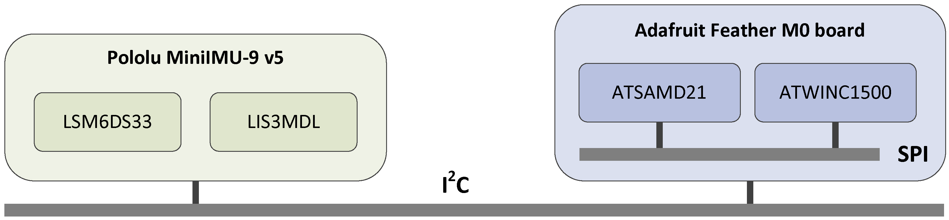
Figure 2.
Three examples of the system implementation with Adafruit Feather M0 board with added Pololu's MinIMU-9 v5 board and other elements such as battery or LED indicators.
Figure 2.
Three examples of the system implementation with Adafruit Feather M0 board with added Pololu's MinIMU-9 v5 board and other elements such as battery or LED indicators.
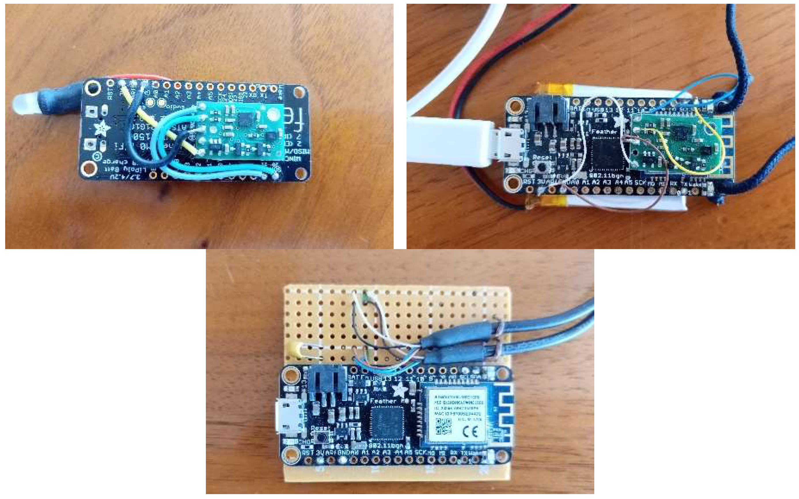
Figure 3.
Implementation of a single timer interrupt serving as a periodic task scheduler.
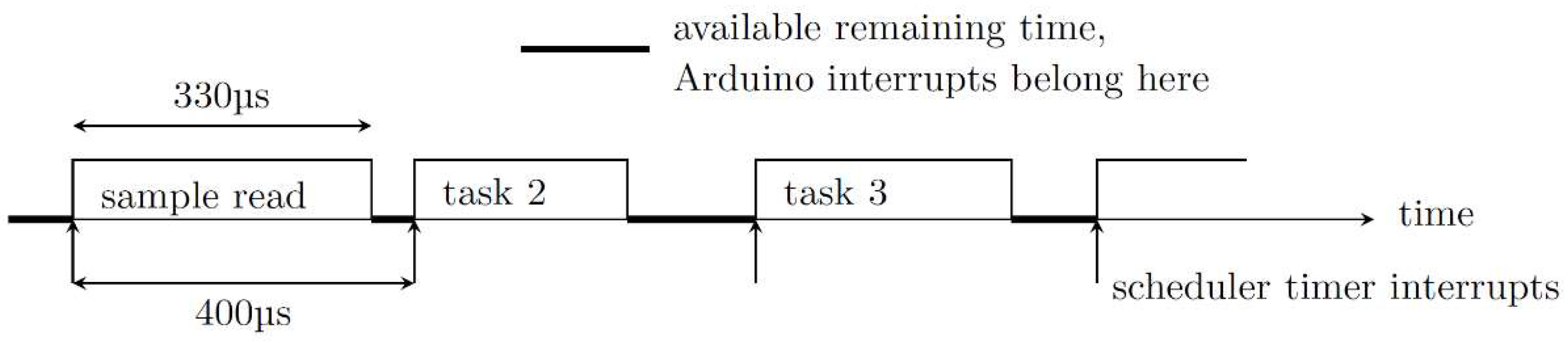
Figure 4.
Operation of the scheduler at two different sampling frequencies and number of samples in a packet. The graph shows (a) the situation with one sensor sample in one packet, (b) the situation with two sensor samples in one packet. Labels R, F, A, and S denote reading, formatting, assembly, and sending tasks, respectively.
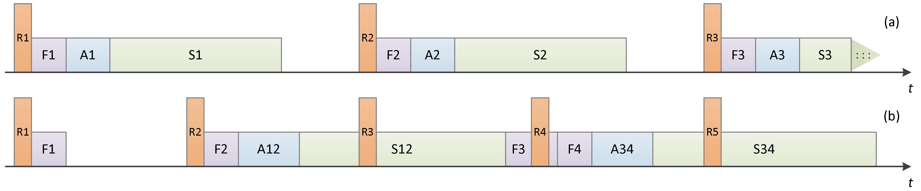
Figure 5.
Oscilloscope traces of Feather M0 board pin states. Pin D1 (lower trace) represents sensor sampling duration, Pin D3 (middle trace) shows packet assembly time, and Pin D4 (upper trace) indicates packet transmission time.
Figure 5.
Oscilloscope traces of Feather M0 board pin states. Pin D1 (lower trace) represents sensor sampling duration, Pin D3 (middle trace) shows packet assembly time, and Pin D4 (upper trace) indicates packet transmission time.
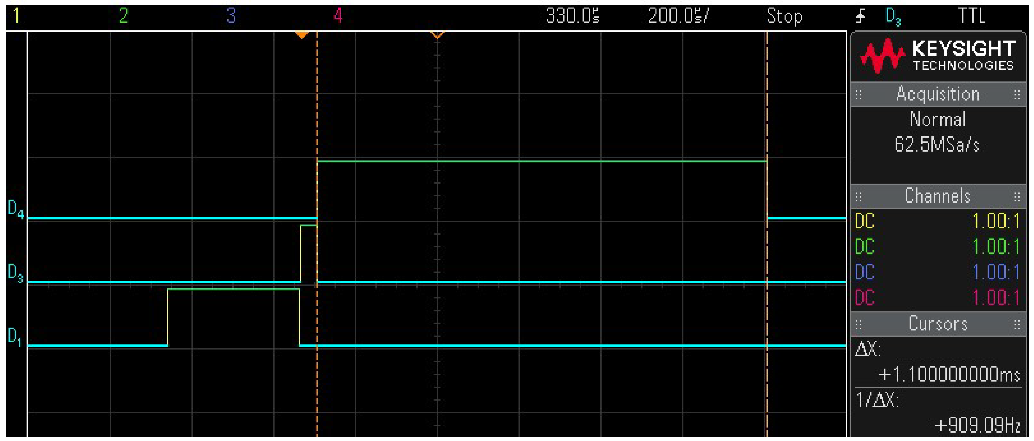
Figure 6.
Four sampling intervals at a 100 Hz sampling frequency with one sample per packet.
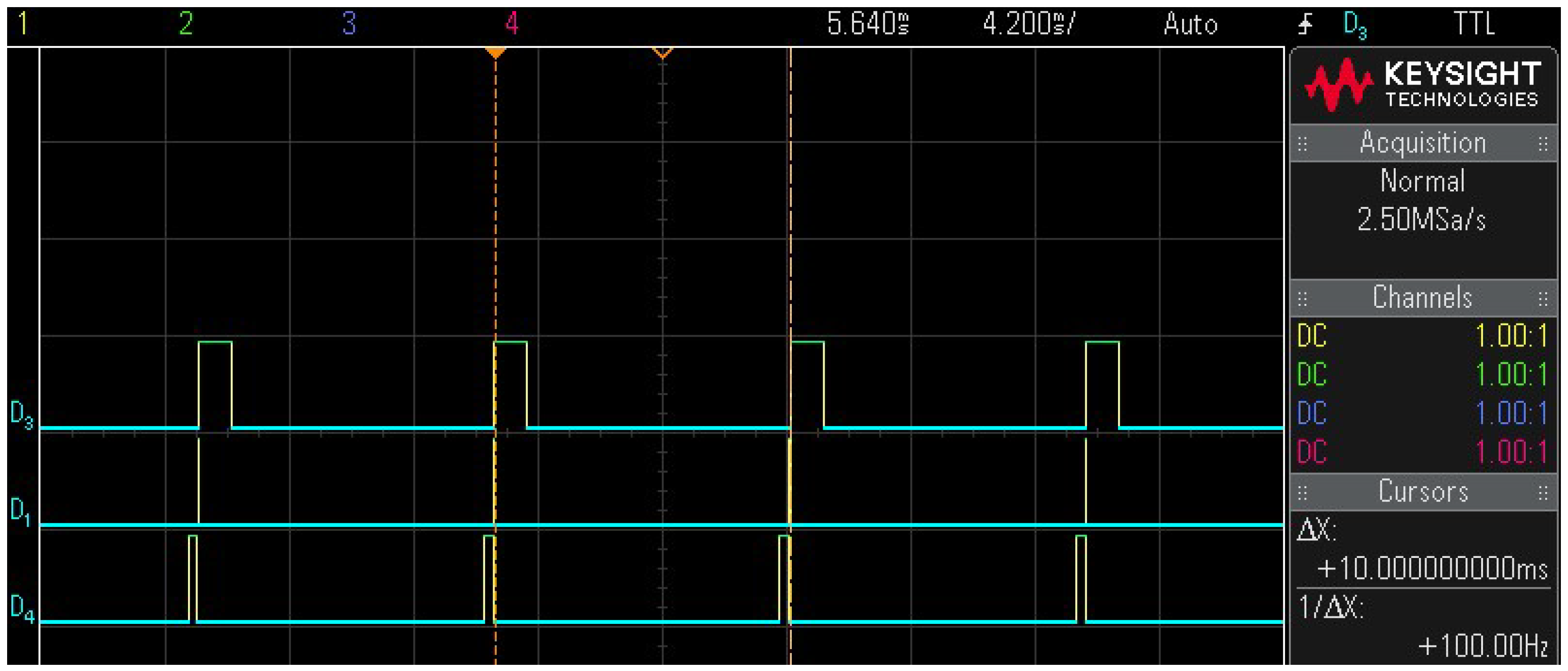
Figure 7.
One sampling episode at a 1750 Hz sampling frequency with 26 samples per packet.
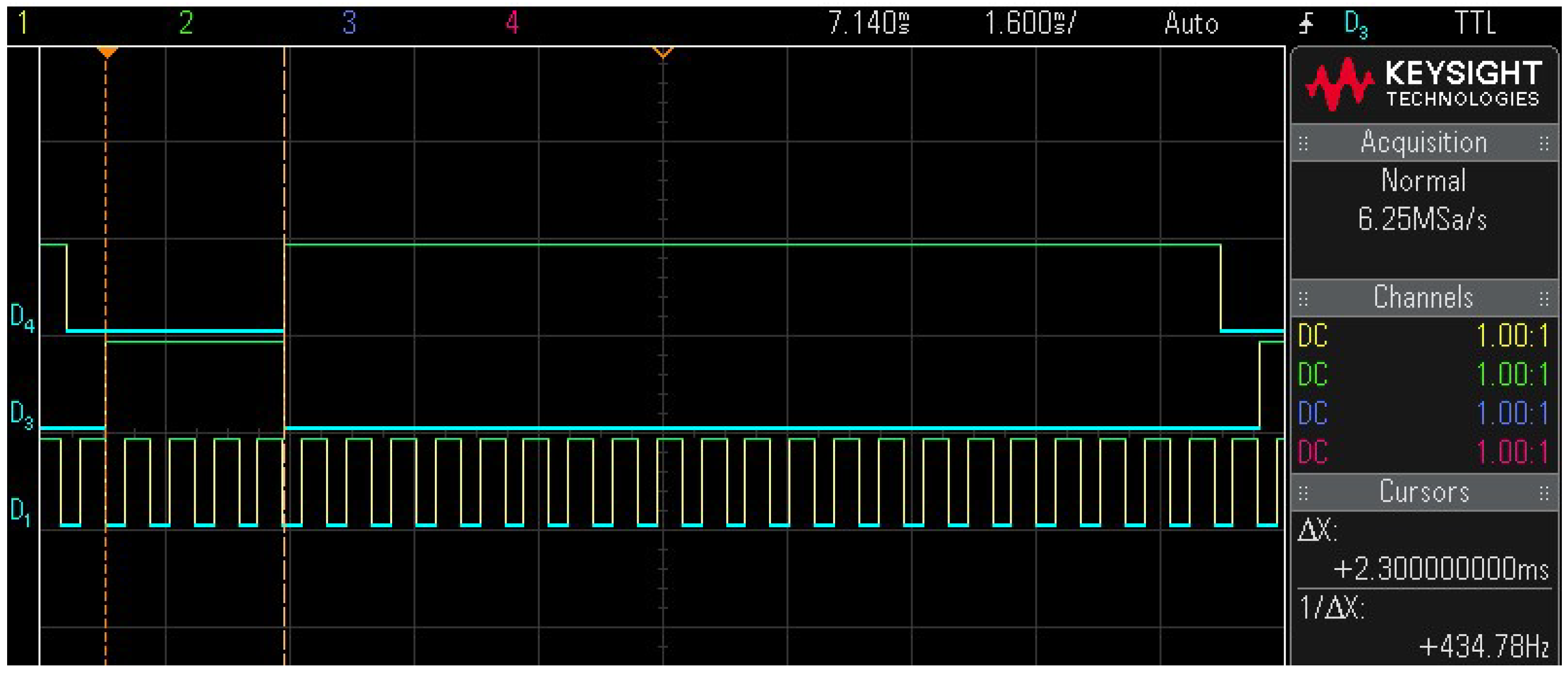
Figure 8.
Sensor readout times versus I²C bus frequency. Values are in milliseconds; the horizontal axis represents frequency in kilohertz.
Figure 8.
Sensor readout times versus I²C bus frequency. Values are in milliseconds; the horizontal axis represents frequency in kilohertz.
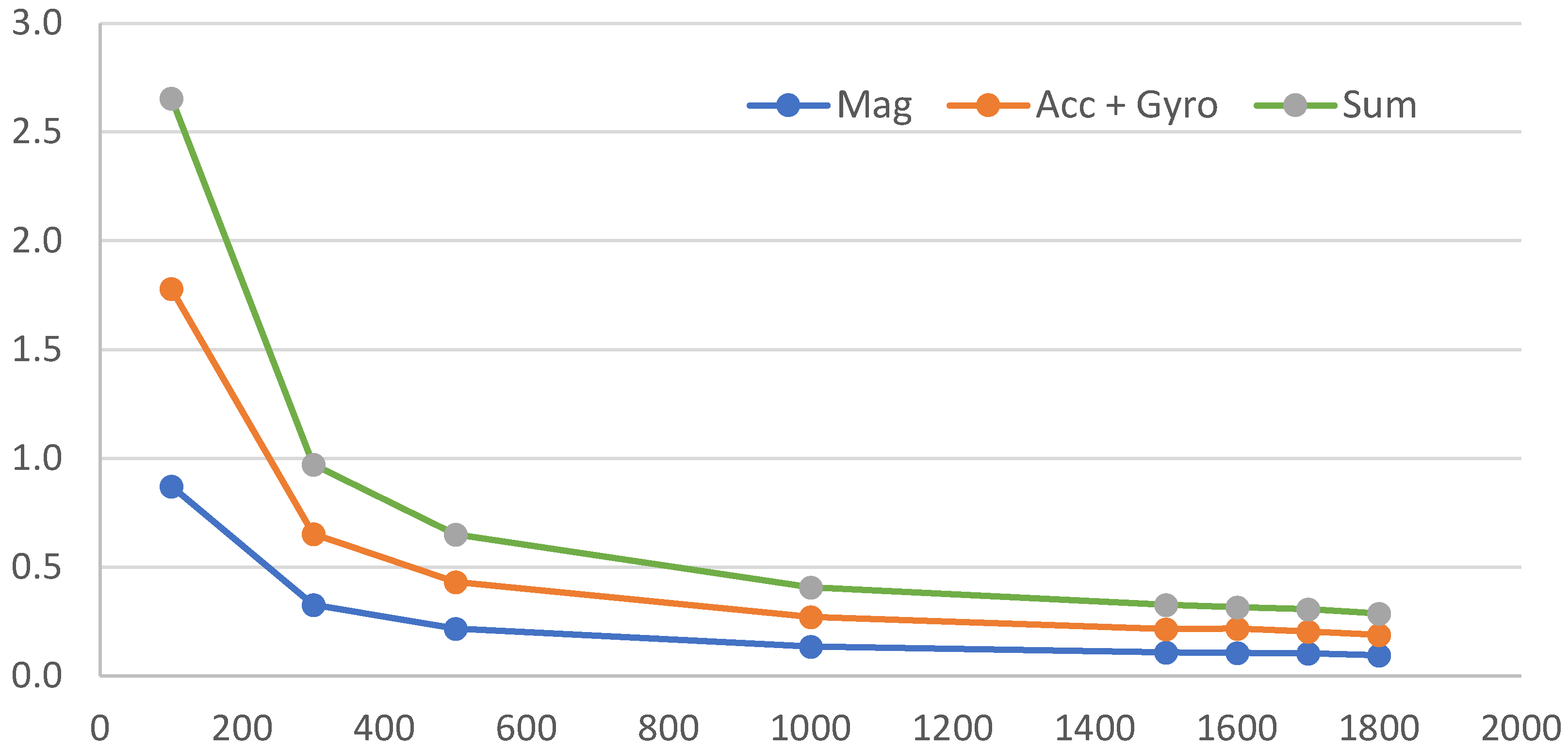
Figure 9.
Packet assembly times [ms] for varying numbers of samples per packet as a function of sensor sampling frequency [Hz], using optimized hexadecimal representation with bit-shifting.
Figure 9.
Packet assembly times [ms] for varying numbers of samples per packet as a function of sensor sampling frequency [Hz], using optimized hexadecimal representation with bit-shifting.
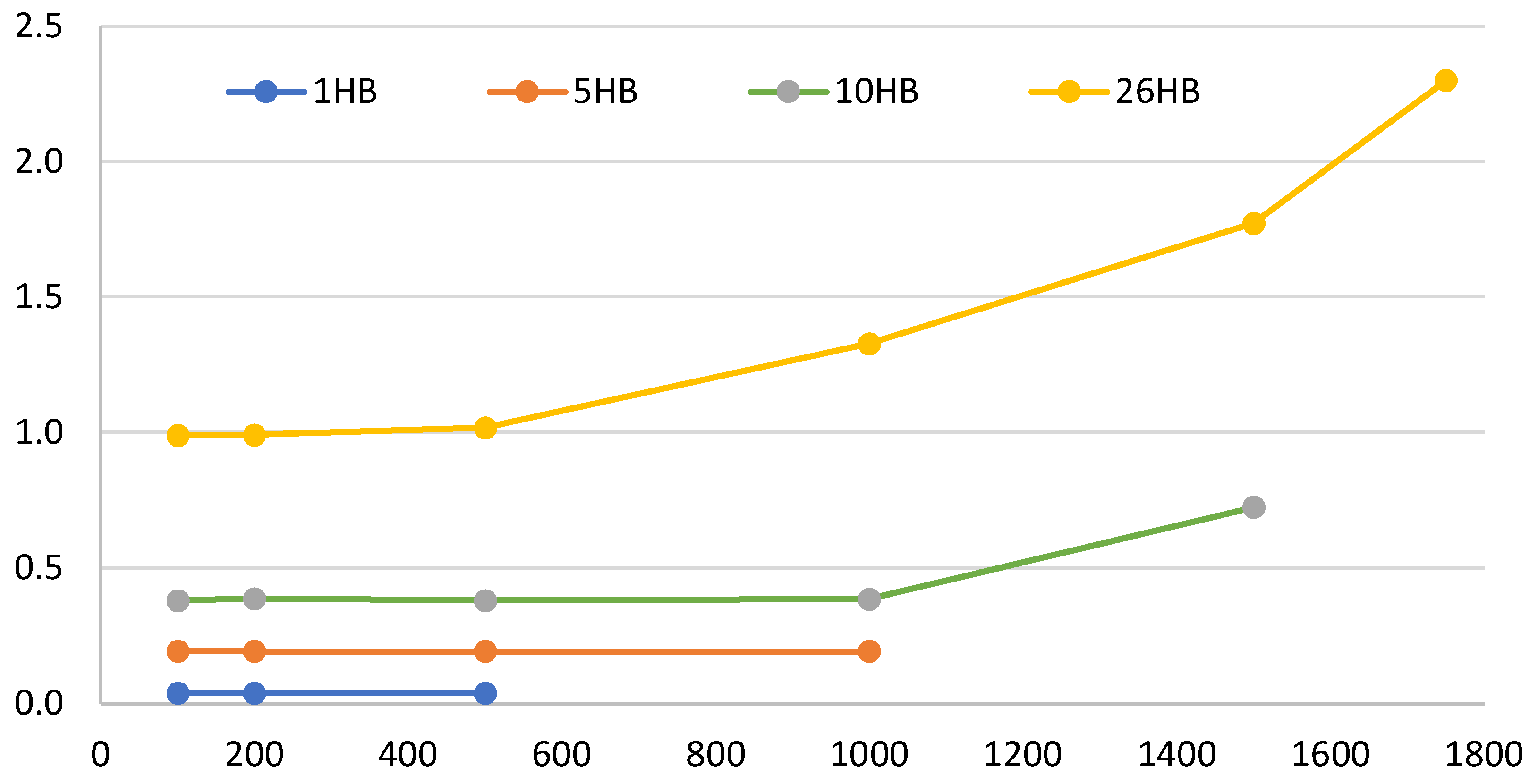
Figure 10.
Packet transmission times [ms] for varying numbers of samples per packet as a function of sensor sampling frequency [Hz], using optimized hexadecimal representation with bit-shifting.
Figure 10.
Packet transmission times [ms] for varying numbers of samples per packet as a function of sensor sampling frequency [Hz], using optimized hexadecimal representation with bit-shifting.
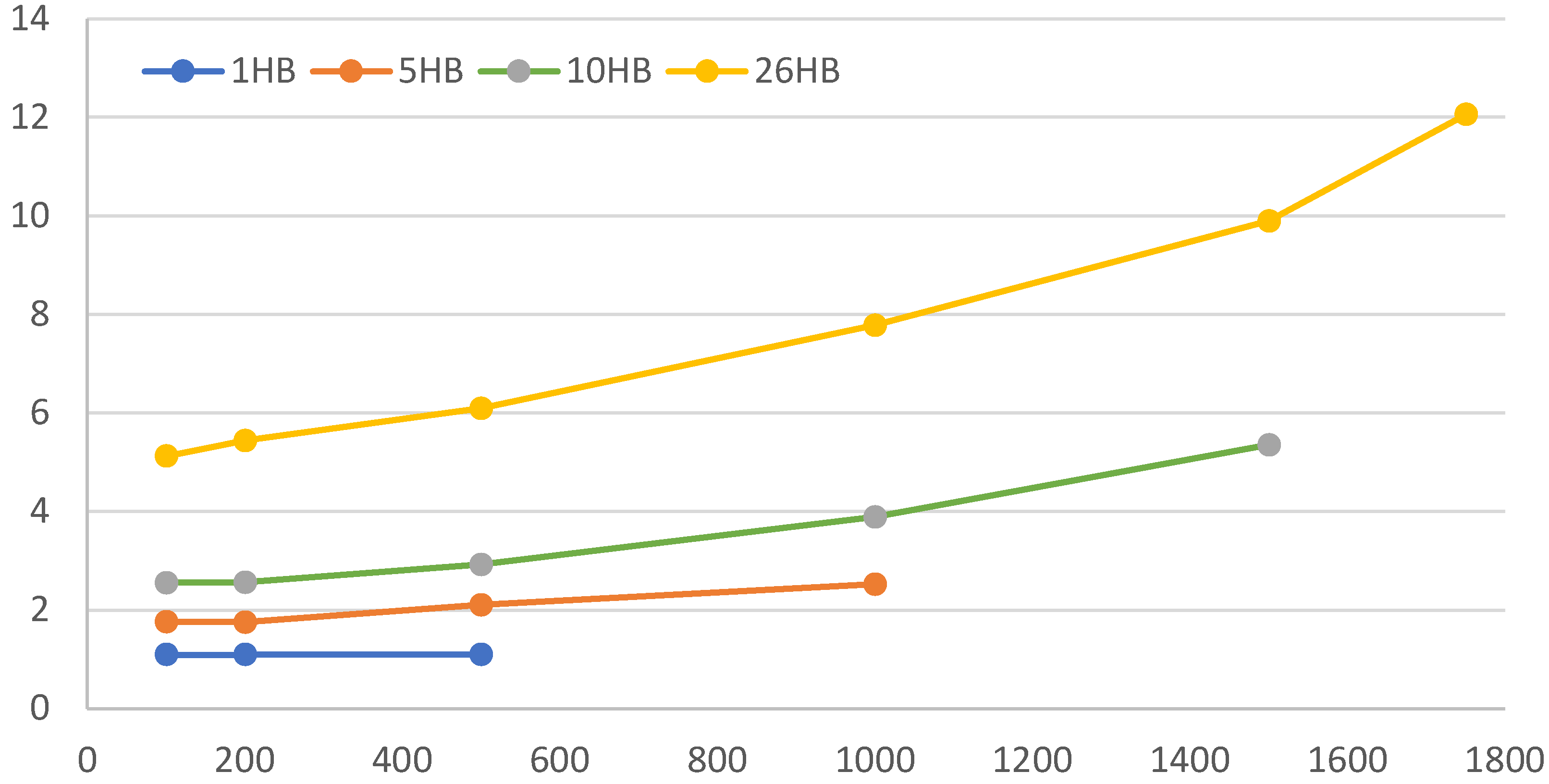
Figure 11.
Average time in [ms] for completion of all tasks needed to send one packet, depending on the sensor sampling frequency. Legend label numbers denote the number of samples in one packet, letters denote different sensor value representations: D = decimal, H = hexadecimal, HS = hexadecimal with a bit shift.
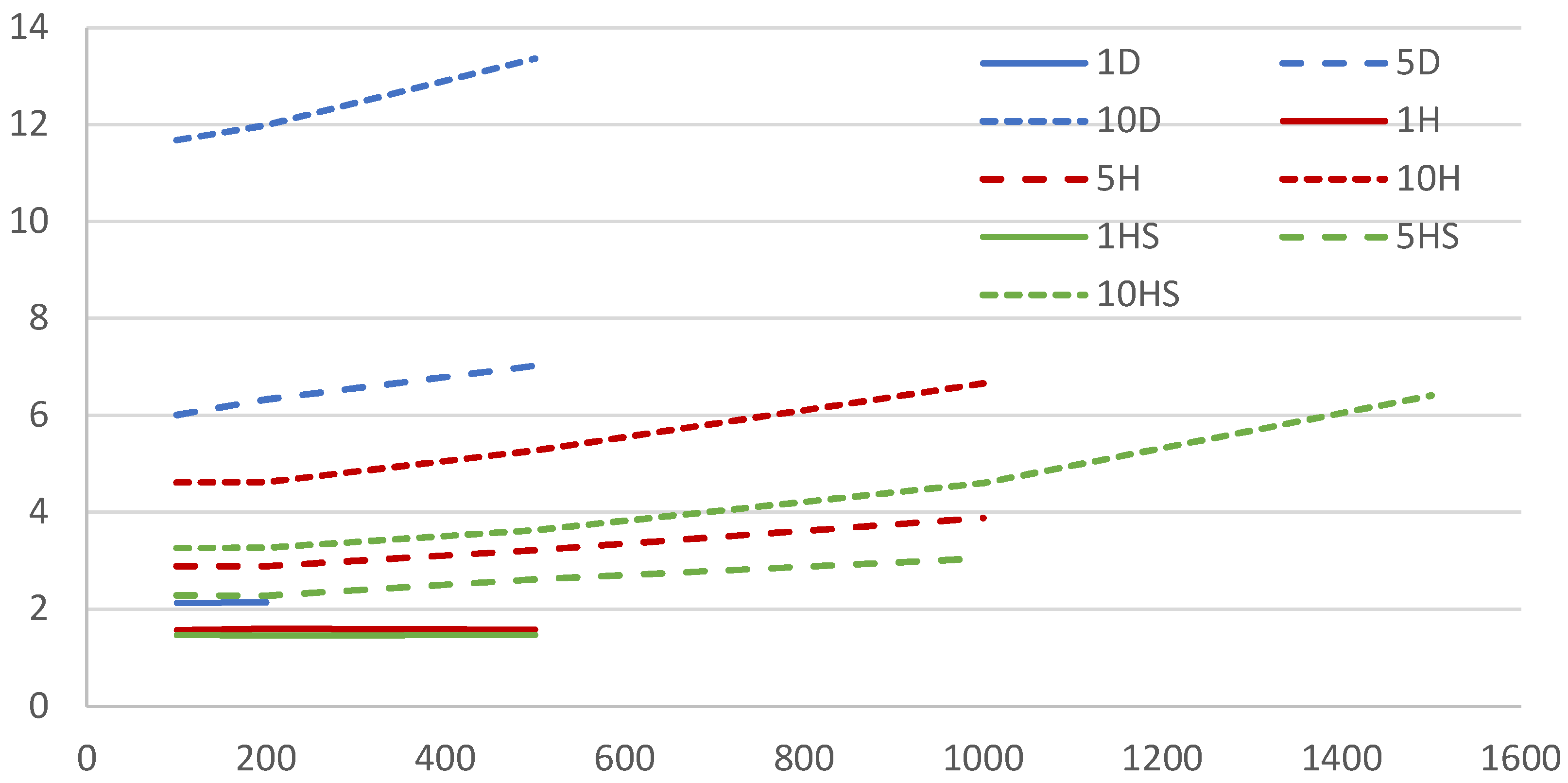
Figure 12.
Average packet delay and jitter [ms] at the receiver as a function of the number of samples per packet at sampling frequency of 100 Hz.
Figure 12.
Average packet delay and jitter [ms] at the receiver as a function of the number of samples per packet at sampling frequency of 100 Hz.


Table I.
Sensor reading times (combined magnetometer, accelerometer, and gyroscope) for four devices at varying I²C bus frequencies [milliseconds].
Table I.
Sensor reading times (combined magnetometer, accelerometer, and gyroscope) for four devices at varying I²C bus frequencies [milliseconds].
| fwire [kHz] | Dev A | Dev B | Dev C | Dev D |
|---|---|---|---|---|
| 100 | 2.640 | 2.680 | 2.650 | 2.650 |
| 300 | 0.972 | 0.972 | 0.976 | 0.972 |
| 500 | 0.642 | 0.676 | 0.646 | 0.642 |
| 1000 | 0.397 | 0.432 | 0.406 | 0.398 |
| 1500 | 0.319 | 0.352 | 0.323 | 0.318 |
| 1600 | 0.306 | 0.339 | 0.314 | 0.307 |
| 1700 | 0.297 | 0.330 | 0.298 | |
| 1800 | 0.288 | 0.288 |
Table II.
Packet assembly times in [ms] for different sensor sampling frequencies fs and different number of samples in one packet in three different formats. A number in column names represents the number of samples and letters the format: D = decimal, H = hexadecimal, HS = hexadecimal calculated by a bit-shift operation.
| fs [Hz] | 1D | 2D | 5D | 10D | 1H | 5H | 10H | 26H | 1HS | 5HS | 10HS | 26HS |
|---|---|---|---|---|---|---|---|---|---|---|---|---|
| 100 | 0.44 | 0.90 | 2.27 | 4.52 | 0.12 | 0.62 | 1.18 | 3.24 | 0.04 | 0.19 | 0.381 | 0.990 |
| 200 | 0.45 | 0.90 | 2.26 | 4.51 | 0.12 | 0.62 | 1.18 | 3.24 | 0.04 | 0.19 | 0.388 | 0.993 |
| 450 | 0.45 | |||||||||||
| 500 | 0.89 | 2.62 | 5.22 | 0.12 | 0.62 | 1.18 | 3.57 | 0.04 | 0.19 | 0.381 | 1.018 | |
| 550 | 0.91 | |||||||||||
| 600 | 2.60 | 5.55 | 0.12 | |||||||||
| 650 | 2.64 | 5.62 | 0.04 | |||||||||
| 1000 | 0.62 | 1.57 | 4.57 | 0.19 | 0.386 | 1.328 | ||||||
| 1150 | 0.95 | |||||||||||
| 1300 | 1.89 | 5.50 | 0.19 | 2.050 | ||||||||
| 1350 | 0.19 | |||||||||||
| 1500 | 0.725 | |||||||||||
| 1550 | 0.713 | |||||||||||
| 1750 | 2.300 |
Table III.
Packet send times in [ms] for different sensor sampling frequencies fs and different number of samples in one packet in three different formats. A number in column names represents the number of samples and letters the format: D = decimal, H = hexadecimal, HS = hexadecimal calculated by bit-shift operation.
| fs [Hz] | 1D | 2D | 5D | 10D | 1H | 5H | 10H | 26H | 1HS | 5HS | 10HS | 26HS |
|---|---|---|---|---|---|---|---|---|---|---|---|---|
| 100 | 1.36 | 1.91 | 3.41 | 6.82 | 1.11 | 1.94 | 3.10 | 8.470 | 1.09 | 1.76 | 2.554 | 5.125 |
| 200 | 1.35 | 1.91 | 3.74 | 7.14 | 1.14 | 1.94 | 3.11 | 8.78 | 1.09 | 1.75 | 2.559 | 5.438 |
| 450 | 1.36 | |||||||||||
| 500 | 2.24 | 4.07 | 7.81 | 1.11 | 2.27 | 3.76 | 9.760 | 1.09 | 2.10 | 2.922 | 6.098 | |
| 550 | 2.25 | |||||||||||
| 600 | 4.41 | 8.18 | 1.12 | |||||||||
| 650 | 4.43 | 8.55 | 1.10 | |||||||||
| 1000 | 2.93 | 4.76 | 12.27 | 2.52 | 3.893 | 7.780 | ||||||
| 1150 | 2.93 | |||||||||||
| 1300 | 5.43 | 14.08 | 3.15 | 12.50 | ||||||||
| 1350 | 3.10 | |||||||||||
| 1500 | 5.355 | |||||||||||
| 1550 | 5.211 | |||||||||||
| 1750 | 12.06 |
Disclaimer/Publisher’s Note: The statements, opinions and data contained in all publications are solely those of the individual author(s) and contributor(s) and not of MDPI and/or the editor(s). MDPI and/or the editor(s) disclaim responsibility for any injury to people or property resulting from any ideas, methods, instructions or products referred to in the content. |
© 2025 by the authors. Licensee MDPI, Basel, Switzerland. This article is an open access article distributed under the terms and conditions of the Creative Commons Attribution (CC BY) license (http://creativecommons.org/licenses/by/4.0/).
Copyright: This open access article is published under a Creative Commons CC BY 4.0 license, which permit the free download, distribution, and reuse, provided that the author and preprint are cited in any reuse.


