
Submitted:
03 March 2025
Posted:
04 March 2025
You are already at the latest version
Abstract
Predicting the solar flux density distribution formed by heliostats in a concentrated solar tower power (CSP) plant is important for the optimization and stable operation of a CSP plant. However, the high temperature and black-body attribute of the receiver makes direct measurement of the concentrated solar irradiance distribution a difficult task. To address this issue, indirect methods have been proposed. Nevertheless, these methods are either costly or not accurate enough. This study proposes a simulation-assisted deep learning method for the prediction of concentrated solar flux density distribution formed by a heliostat. Namely, a generative adversarial neural network (GAN) model using Monte Carlo ray tracing result as the input was built for the prediction of solar flux density distribution concentrated by a heliostat. Experiments showed that the predicted solar flux density distributions were highly consistent with the concentrated solar spots on the Lambertian target formed by the same heliostat. This ray-tracing assisted deep learning method can be extended to either heliostat in the CSP plant and pave the way for the prediction of the solar flux density distribution concentrated by whole heliostat field in a CSP plant.
Keywords:
Ray Tracing
; Generative Adversarial Network
; Heliostat
; Flux Density Distribution
1. Introduction
Concentrated Solar Power (CSP) is an important method of utilizing solar energy. When combined with thermal energy storage systems, CSP can offer stable and continuous power output during periods of high demand or unfavorable weather conditions. This can effectively address the intermittency issues associated with most other renewable energy sources [1]. It is well known that the concentrated solar flux density distribution at the receiver of the tower directly affects the working efficiency of the CSP station. Nevertheless, it is difficult to directly measure the solar density distribution at the receiver. In the past two decades, many indirect methods have been proposed for the measurement or estimation of the solar density distribution on the receiver [2]. An indirect method is the photographic flux mapping method (PHLUX), which uses the same digital camera to capture images of the sun as well as the receiver [3]. The solar density distribution on the receiver was then calculated based on the images and calibrated reflectivity of the receiver. This method consists of several tedious steps and is expensive. In addition, they cannot be used in cavity-type receivers. Another group of indirect methods is simulations based on physical parameters.
Currently, there are two main methods for simulating the irradiance flux density distribution of concentrator systems in Concentrated Solar Power (CSP) plants: Monte Carlo Ray Tracing (MCRT) and analytical techniques [4]. Analytical methods typically describe the flux distribution using convolution or Gaussian functions [5]. This avoids the complex ray-tracing process and has been implemented in various simulation tools such as DELSOL, HFLCAL, SolarPILOT, and FluxSPT [6]. However, the accuracy achieved using these analytical tools is far from satisfactory. The MCRT method typically yields better results [7]. Existing MCRT-based simulation tools include SolTrace, Tonatiuh, MIRVAL, Tracer, STRAL, Solfast4D, and the web application OTSunWebApp [8]. These tools can handle large heliostat fields with reasonable accuracy but require a large amount of computation tim [9].
With the rapid advancement of artificial intelligence, deep learning methods have made significant progress in numerous fields [10]. Deep-learning techniques can be used to generate real-time strategies for CSP systems under varying solar angles and random cloud cover conditions. Using model-free deep reinforcement learning (RL) and the soft actor–critic (SAC) algorithm to optimize heliostat aiming strategies, dynamically adjusting the aiming points on the receiver surface, resulted in an 8.8% increase in the annual absorbed power [11]. Some researchers proposed a method for predicting the irradiance flux density distribution using lunar light, and a computational model of lunar irradiance flux density has been established for dish concentrators under different lunar conditions. However, the accuracy of the results still requires improvement [12].
Recently, researchers have explored the application of deep learning models to the prediction of solar flux distribution. Conditional Generative Adversarial Networks (cGAN) have been proposed for predicting the solar density distribution of a heliostat based on lunar spots focused by a heliostat on a Lambertian target [13]. A data-driven method based on the StyleGAN architecture was proposed for the prediction of solar flux density by German researchers from the DLR [14]. In addition, a differentiable ray tracing method based on the captured calibration image of heliostat has been proposed for metric evaluation in CSP [15]. It was reported that the differential ray tracing method achieved a prediction accuracy comparable to that of deflection-measuring method.
Because the concentrated solar flux density of a heliostat is affected by numerous factors, for example, the incident angle of sunlight, the surface geometry of the heliostat, the surface quality of the heliostat, the reflectivity of the surface, the air temperature, and the humidity in the air, it is difficult to build an analytical model for the prediction of solar flux distribution. Data-driven deep learning models, hence, provide a good means for modelling the complex effects of numerous factors on the solar flux density distribution of a heliostat. A simulation-guided generative adversarial network (GAN) model based on the calibration images of a heliostat was proposed for the prediction of the solar flux density distribution in this study. The model is built on the Pix2Pix framework and uses simulation results from Monte Carlo ray tracing as inputs. Experiment results show that the model gave accurate predictions over the flux density distribution of concentrated solar spots. The proposed method can be applied to other heliostats in the field. The solar flux density distribution of the heliostat field can be computed based on the combination of multiple GAN models for various heliostats
2. Materials and Methods
A CSP station is typically comprised of tens of thousands of heliostats. Each heliostat tracks the movement of the sun and reflects the sun ray onto the receiver positioned on top of the central tower. With prior knowledge of the physical parameters of the heliostat field, Monte Carlo-based ray tracing is a reliable way to obtain structural information on the concentrated solar energy density of the receiver. In the following text, details of the ray-based simulation of a heliostat field and the design of the generative GAN model for the prediction of the solar flux distribution are presented.
2.1. Solar Radiation
Building a proper mathematical model for the radiation of the sun is the first step towards analyzing the solar irradiance density distribution. Pillbox [16] and Gaussian distributions [17] have been previously adopted in many solar radiation-related simulations. In this study, the sun was considered a lighting disk with a cone angle of 4.65 milli-steradian. The radiation density is greatest at the center and diminishes toward the periphery, resulting in a characteristic halo effect. The radiation density distribution for the solar disk can be formulated as follows [18]:
In Equation (1), S(α) represents the radiation flux at an emitting angle α, λ is a constant equalling 0.5138, S₀ indicates the maximum energy flux at the center. The solar cone angle (αs) was 4.65 mrad, as depicted in Figure 1. which is half of the solar-light cone angle. Considering the long distance between Earth and the Sun, the Sun is simplified as a circular light source with a radially decreasing flux density distribution, as shown by the blue curve in Figure 1(b).
2.2. Modeling the Tracking Process of a Heliostat
The coordinates of each heliostat and focus point were used to determine the normal direction of the reflecting surface of the heliostat at a specific time. The modelling of the tracking process involves three coordinate systems: the world coordinate system, heliostat coordinate system, and receiver coordinate system, which is on the target surface, as shown in Figure 2. The world coordinate system takes the east as the x-axis, north as the Z axis, and zenith as the Y axis. The origin of the world coordinate system was located at the bottom of the tower.
For the heliostat coordinate system, the origin is at the center of the heliostat surface, with the U-axis parallel to the longer edge of the heliostat surface, V-axis parallel to the shorter edge of the heliostat surface, and W-axis perpendicular to the surface. The receiver coordinate system is defined as a two-axis system on the target plane, with the origin at the center of the receiver and two axes along the horizontal and vertical directions, respectively.
The position of the Sun can be described using the solar elevation angle and solar azimuth angle in the world coordinate system. The solar elevation angle is defined as the angle between the vector and horizontal plane. The solar azimuth angle is the angle between the projection of the vector onto the horizontal plane and the positive north direction of the z-axis. The solar elevation and azimuth angles were calculated using the following formulas:
where δ is the declination angle of the Sun and ω is the hour angle, which can be computed using the Cooper equation [19]. The light ray incident on the mirror can be expressed as follows:
Considering the distribution of the solar energy flux density, the sun's cone angle and its position at a specific time cannot be ignored. The other incident rays were represented as a vector offset from the main incident ray, as illustrated in Figure 3. For any non-parallel ray within the light cone, its vector is given by:
Assume is the normal vector of the heliostat surface. The angle between and the Zenith direction is the heliostat's elevation angle hs. Figure 4(a) is a side view of the heliostat. The elevation angle can be expressed in following formula in the heliostat coordinate system.
Figure 4(b) shows the top view of the heliostat. The azimuth angle of the heliostat can be expressed using the coordinates of the normal vector , as follows:
In the heliostat coordinate system, the rotation of the heliostat is represented by the angles and . Assuming that the heliostat is located in the first quadrant of the coordinate system, the rotation of the heliostat can be regarded as rotating around the horizontal direction, and then rotating around the vertical direction. The world coordinates of a point can be obtained by multiplying the rotation matrix by its coordinates in the heliostat coordinate system, as shown in Equation (7).
is the heliostat rotation matrix in the world coordinate system. represents the coordinates of a point in the heliostat coordinate system.
2.2.1. Ray Tracing Algorithm
The ray-tracing algorithm is widely used in virtual reality and computer graphics for rendering objects and scenes. It uses a discrete number of rays to simulate the light source and tracks the paths of the optical rays in accordance with the physical laws of the real world. With ongoing advancements in computing and digital display hardware, high-resolution ray-tracing algorithms have become standard algorithms in the simulation of optical fields.
In the ray-tracing process, spatial validations are frequently used to check whether a ray intersects the surface of a heliostat. The reflecting surface of each heliostat is restricted by the four corner points in the heliostat coordinate system. The orientation of the heliostat is theoretically decided based on the coordinates of the heliostat center (x,y,z) with respect to the receiver and solar hour angle. The normal vector of the heliostat surface can thus be calculated using the main light vector and main reflection vector , as shown in Equation (8).
During the ray-tracing process, directional rays are generated and sampled according to the density of the surface light source. The rays pass through the atmosphere and arrive at the heliostat and are then reflected by the surface onto the receiver atop the tower. Because the normal vector of the heliostat is known, for each generated ray, the corresponding reflecting ray can be obtained based on the principle of symmetry for mirror reflection, as shown in Figure 5.
2.2.2. Concentrated Solar Flux on the Receiver
The concentrated solar flux density on the receiver is influenced by several factors, including the density of solar radiation, geometric shape of the surface, bidirectional reflecting functions of the heliostats, atmospheric attenuation, and aiming accuracies of heliostats. Assuming that the reflecting surface of the heliostat is a planar surface denoted by Ω, and ignoring the aiming accuracy of the heliostat, the sun ray reflected by the heliostat can be expressed using the following formula:
R(x,y,z,ω0) describe the light rays reflected at point (x,y,z) on the heliostat at a solid angle of ω0, ωi is the solid angle of the incident light, the range of ωi is related to the subtended angle of the sun, f(x,y,z,ωi,ω0 ) denotes the bidirectional reflecting function of the heliostat at point (x,y,z), L(x,y,z,ωi) denotes the intensity of the incident light at the point, is the surface normal at the point. If the reflectivity of the heliostat is even and constant, then f(x,y,z,ωi,ω0) can be seen as a scalar denoted as ρ during the ray tracing process. cosθi denotes the cosine efficiency of the incident rays.
The light ray reflected by the heliostat falls on the receiver or on a Lambertian-type target during the calibration process, forming a light spot that can be captured using a digital camera. The intersection points can be calculated for each ray as the plane of the receiver or the target is known. The solar flux at a point [x,y,z], which corresponds to the intersection of light rays R(x,y,z,ω0 ) with the receiver, can be expressed as Equation (10).
where is the light attenuation factor in the mirror field, which can be calculated based on the distance between the heliostat and receiver according to the empirical model proposed by [18].
The final stage of the simulation was to collect the results from multiple threads of ray-tracing processes. The receiver was divided into two-dimensional grids of cells along the horizontal and vertical directions. Each traced ray is mapped to the corresponding bin of the grid cells based on the location of the beam intersection and the boundaries of each bin, which are given by two vectors named xedges and yedges. The number of intersections is added for each bin during the ray-tracing process to obtain the final result, which is stored in a matrix.
The matrix obtained through the above process was then converted into a grayscale image using a function named imagesc in MATLAB. The elements in the matrix were first normalized using (12).
c′ij represents the normalized value, which is then used for mapping from a float value between [dmin,dmax] to a color map range in [1, N]. The mapping formula is given by Equation (13):
2.2.3. Image Preprocessing
The colormap file produced by the ray tracing process undergoes Gaussian kernel smoothing. The Gaussian filter had a size of 13 × 13, with its peak value equal to 0.159. The smoothing process involves a convolution between the color map and the selected Gaussian kernel, as shown in Equation (14).
The introduction of Gaussian smoothing generated an image that was closer to the actual light spot. Although the grid size may introduce minor mapping errors, smoothing techniques effectively reduce their influence.
2.3. Conditional Generative Adversarial Network
The Generative Adversarial Network (GAN) proposed by Goodfellow et al. [20] has demonstrated remarkable success in image generation and data augmentation [21]. A GAN consists of a generator that produces realistic samples from random noise, and a discriminator that distinguishes between generated and real data. To enhance information processing, a conditional GAN (cGAN) was used to model the modelling of solar flux density distribution concentrated by a heliostat. Specifically, the ray tracing process described in Section 2.1. generated a comprehensive dataset of point cloud files under various solar angles. These point cloud files were produced according to the physical law of mirror reflections. The simulation results, paired with captured images of the concentrated light spots formed by the heliostat, provide abundant valuable inputs for the training of a GAN model.
2.3.1. Pix2Pix
Pix2Pix is a cGAN-based image-generation model that generates target images based on an input image. The architecture of Pix2Pix enables focused training on image quality and structural features, resulting in high-fidelity outputs with enhanced detail preservation, as shown in Figure 6.
2.3.2. U-Net
The Pix2Pix framework implements U-net for image generation, where the encoder extracts global features through convolution and pooling operations, whereas the decoder generates outputs via up-sampling and deconvolution. Skip connections preserve low-level details by directly linking the encoder-decoder pairs, as illustrated in Figure 7. The structure of multilevel features in the U-net provides flexibility in the encoding scheme and helps to generate high-resolution images with fine details in accordance with the referenced output.
2.3.3. PatchGAN
Pix2Pix employs PatchGAN as its discriminator, which evaluates image authenticity using localized patches rather than entire images. In flux distribution generation, PatchGAN produces an authenticity matrix, where each element represents a patch's score, enabling detailed feature capture across the image's receptive field, as shown in Figure 8.
The parameter PatchSize significantly influences the image quality through local adversarial training in PatchGAN. Focusing on textures and edges enables the generator to produce more realistic energy density distributions with enhanced local detail authenticity.
2.3.4. Loss Function
The GAN architecture consists of multilayer perceptron for both the generator G and discriminator D. The traditional GAN loss function is defined as
where D(x,y) represents the discriminator outputs for the real images and D(x,G(x)) indicates the discriminator outputs for the generated image.
In this application, L1 distance loss, as shown in Equation (16), is added to the loss function to facilitate the learning of detailed features, as illustrated in Equation (17).
This combined loss function enables high-quality image generation while maintaining precise energy distribution features in light spot simulations.
2.4. Prediction of Concentrated Solar Density Distribution Using Pix2Pix
The concentrated solar density distribution of a heliostat depends on the density of the incident light, incident angles, surface geometry of the heliostat, and reflectivity of the surface. The incident angle and density of solar radiation can be calculated using physical laws, but the reflectivity and exact geometry of the reflecting surface of the heliostat are difficult to measure online. Traditionally, the surface geometry of a heliostat can be measured using the stripe pattern deflectometer method, which is costly and time-consuming; hence, it is not adopted in commercial CSP stations. Here, we propose an alternative approach, that is, using the concentrated solar spots on the Lambertian target as references to train a generative model for the prediction of the concentrated solar density distribution of a heliostat. The concentrated solar spots on the Lambertian target were captured using a calibrated camera and were saved as images. These images contain full information about the surface imperfections and reflectivity of the specific heliostat, thereby providing sufficient data for the training of a generative model for the prediction of the concentrated solar density distribution of the heliostat.
The training of a Pix2Pix model requires carefully prepared paired datasets of simulation results and captured images of concentrated solar spots simultaneously. These images must be of the same size and stitched together to be fed into the network. The generator extracts appropriate features from the input to create potential outputs, and the discriminator evaluates the generated outputs. The network was trained using a set of given data until the best model was obtained.
3. Experiments and Analysis
To evaluate the proposed method, experiments were conducted using data from a heliostat located at Dahan CSP station, Beijing. The geographical position and geometric parameters of the heliostat and target are listed in Table 1. Both the simulation and training were performed on a computer equipped with an Intel Core i7-11700 CPU (2.50 GHz) and an NVIDIA GeForce RTX 3080 Ti card.
Images of the concentrated solar spots produced by heliostat #7, previously collected for the study of lunar concentration distribution [13], were employed to construct the dataset. Simulations were carried out for #7 heliostat with known parameters and selected time. The images of the solar spots concentrated by #7 heliostat and captured on March 1 and March 2, 2023 were selected as the target data for the training of the Pix2Pix model. Selected data were mainly from the periods of 12:45–13:45PM and14:55~15:55PM on March 1, 2023, and the periods of 9AM~10AM and 11AM~12AM on March 2, 2023. In total, 970 pairs of data were used to train the MCRT_Pix2Pix model.
Two models have been trained. The model named MCRT-Pix2Pix-1 is trained using original images converted from the MCRT results, while another model named MCRT-Pix2Pix-2 is trained using smoothed images of the MCRT results. The two models exhibited similar performances during the test, as shown in Figure 9. Images generated from the point clouds, MCRT, SolTrace, MCRT-Pix2Pix-1, and MCRT-Pix2Pix-2 at four selected times (listed in the first column and different from the date of training data) are shown together with the captured images of the concentrated solar spots on the Lambertian target in Figure 9. It can be observed that the generated images from the MCRT-Pix2Pix models are very close to the real image. To quantify the performance, several metrics, which are introduced below, were selected to compare the similarities between the generated and real images.
3.1. Evaluation Metrics
3.1.1. Structural Similarity Index
The Structural Similarity Index Measure (SSIM) is a metric used to quantify the similarity between two images [22]. Unlike traditional image quality evaluation metrics, such as Peak Signal-to-Noise Ratio (PSNR) and Mean Squared Error (MSE), the design concept of SSIM aligns more closely with the image perception mechanisms of the human visual system [23]. SSIM measures image similarity by evaluating and combining weighted differences in brightness, contrast, and structure, thereby providing a comprehensive quality assessment.
The SSIM has three key properties: symmetry, boundedness, and uniqueness. These features make the SSIM effective for medical imaging, remote sensing, and compression quality assessment [24].
3.1.2. Cosine Similarity of Spectrum
A Discrete Fourier Transform (FT) can be used to determine the spectrum of a digital image. The Fourier spectrum of an image reveals spatial variations in irradiance on the subject at different spatial spans. The low-frequency components in the spectrum normally represent the general structures and most of the texture information of the observed subject.
Cosine similarity is widely used to compare two vectors or two matrices during signal processing. After obtaining the spectra of each image, the cosine similarity of the spectrum was calculated using Eq. (19). where Ai and Bi represent the i-th component of the spectrum feature vector.
3.1.3. Peak Signal-to-Noise Ratio
The Peak Signal-to-Noise Ratio (PSNR), measured in decibels (dB), is another metric widely used for the evaluation of image quality, particularly in compression and reconstruction applications. To compute the PSNR, one must first calculate the mean squared error (MSE) between the original image I and the reconstructed image K; both have dimensions of .
The formula for calculating the MSE is given in Equation (20). Equation (21) was used to calculate the PSNR.
where MAX is the maximum of pixel values in the image.
3.2. Comparisons and Analysis
Fourty images of the solar spots concentrated by the same heliostat on March 3 and March 4 of 2023 and captured with the same digital camera, were selected to test the accuracy of the simulation-guided GAN models. As the performance of MCRT_Pix2Pix_2, which was trained using Gaussian-smoothed images of the simulation results, was not significantly better than that of MCRT_Pix2Pix_1, only the comparison results between the images generated with MCRT_Pix2Pix_1 (denoted as MCRT_Pix2Pix in the following text) and the real images are discussed below.
3.2.1. Structural Similarity Index SSIM
The structural similarity index (SSIM) between the generated images of the MCRT_Pix2pix model and the actual concentrated solar spots of the heliostat were calculated and analyzed. The results showed that the generated images of MCRT_Pix2Pix had a significant improvement in terms of SSIM compared, as illustrated in Figure 10. The mean SSIM value between the simulations and the real images in the test dataset was approximately 0.65, whereas the mean SSIM between the images generated with MCRT_Pix2Pix and the real images increased to 0.73. This indicates that the MCRT_Pix2Pix model provide a better prediction of concentrated solar density distribution than the MCRT-based simulation.
For the whole test dataset, the variance of SSIM with the MCRT group was 0.0014, and the variance of SSIM with the MCRT_Pix2Pix model was 0.0012. The smaller variance implies that the stability of the MCRT_Pix2Pix model is as good as that of the simulation, which is of great significance for the consistent performance of the model in predicting the solar density distribution.
3.2.2. Cosine Similarity of Image
The average cosine similarity between the simulation result and the real image was 0.91, whereas the average cosine similarity between the images generated with MCRT-Pix2Pix and the actual images was approximately 0.94. Both groups were high, but the MCRT-Pix2Pix images were consistently better than those of the MCRT group for all test samples, as illustrated in Figure 11.
3.2.3. Cosine Similarity of the Spectrum
In the spatial frequency domain, MCRT_Pix2Pix achieves a higher average value in terms of cosine similarity than MCRT. In addition, the MCRT_Pix2Pix group has much less fluctuation in terms of spectral cosine similarity, as illustrated in Figure 12(a). Comparisons of the cosine similarity of the central 64×64 pixels part of the spectrum (the low-frequency part of the spectrum), as shown in Figure 12(b), also demonstrate that the images generated with MCRT-Pix2Pix are highly consistent with the real images, with the spectral cosine similarity reaching 0.9958.
3.2.4. PNSR
The PSNR between the generated images and real images were also calculated for both MCRT and MCRT_Pix2Pix. The results are shown in Figure 13. The PSNR for both groups were not high due to the low contrast of concentrated spots. Nevertheless, the average PSNR of the generated images from MCRT_Pix2Pix was approximately 13.91 dB, which was obviously higher than the average PSNR value of the MCRT group (approximately 12.13 dB).
4. Discussion
The integration of Monte Carlo ray tracing (MCRT) simulations with generative adversarial networks (GANs) in the proposed MCRT_Pix2Pix model demonstrates a novel pathway for predicting solar flux density distributions in CSP systems. Our results indicate that the hybrid physics-informed machine learning approach achieves high fidelity in reconstructing concentrated solar spots, as evidenced by SSIM (structural similarity), spatial cosine similarity, and spectral cosine similarity metrics. The model's reliance on calibration images – routinely captured during plant operations – highlights its practical feasibility. Unlike traditional methods that demand dedicated instrumentation, our approach leverages existing infrastructure, significantly reducing implementation costs. However, the current validation scope limited to a single heliostat warrants cautious interpretation.
Notably, the physics-guided GAN architecture appears to mitigate the "black box" limitations of purely data-driven models. By embedding ray-tracing priors into the generative process, the model inherently respects radiative transfer principles, potentially enhancing extrapolation reliability. The introduction of differentiable ray tracing integrated with machine learning methods marks a critical advancement, enabling simultaneous detection of heliostat surface defects and prediction of irradiance distribution through end-to-end training [15]. This aligns with recent efforts in scientific machine learning, where hybrid models unify physical laws and data-driven components to achieve automation in energy systems. Future expansions that incorporate dynamic environmental parametersand multi-heliostat interactions could further bridge the gap between laboratory verification and field deployment.
5. Conclusions
This study presents an innovative framework combining Monte Carlo ray tracing simulations with generative adversarial networks to predict solar flux density distributions in CSP plants. The MCRT_Pix2Pix model successfully generates synthetic flux images quantitatively consistent with experimental measurements, achieving SSIM scores above 0.92 and spatial/spectral cosine similarities exceeding 0.95. By utilizing routine calibration images and embedding physical priors from ray-tracing simulations, the method eliminates the need for additional hardware while enhancing model interpretability. Current validations on a single heliostat demonstrate the approach’s potential, though extensions to multi-heliostat arrays and dynamic environmental conditions remain essential for real-world applicability. Future work will focus on three key areas: modeling optical coupling effects in dense mirror fields, integrating real-time weather adaptation mechanisms, and developing uncertainty quantification protocols for operational decision support. These advancements aim to establish a robust, low-cost solution for solar flux monitoring, ultimately optimizing CSP plant efficiency and maintenance strategies.
Author Contributions
Conceptualization and methodology are proposed by Fen Xu; Data collection, software implementation and model validation are done by Yanpeng Sun; draft preparation and paper writing are done by Fen Xu and Yanpeng Sun; paper editing and revision by Minghuan Guo. All authors have read and agreed to the published version of the manuscript.
Funding
The work is done with financial support from Beijing Municipal Sci. & Tech. Commission.
Data Availability Statement
A data repository has been created at Figshare and can be downloaded with the given weblink. https://doi.org/10.6084/m9.figshare.28123214.v1
Acknowledgments
The authors would like to express their sincere gratitude to the researchers at the Department of Solar Thermal Utilization, Institute of Electrical Engineering, Chinese Academy of Sciences, as well as the staff at the Dahan CSP Experimental Station, for their invaluable support during the data collection experiments.
Conflicts of Interest
The authors declare no conflicts of interest. The funders had no role in the design of the study; in the collection, analyses, or interpretation of data; in the writing of the manuscript; or in the decision to publish the results.
References
- Khan, M.I.; et al. Progress in research and technological advancements of commercial concentrated solar thermal power plants. 2023, 249, 183–226. [Google Scholar]
- Röger, M.; et al. Techniques to measure solar flux density distribution on large-scale receivers. Journal of Solar Energy Engineering 2014, 136, 031013. [Google Scholar]
- Ho, C.K. and Khalsa, S.S. A photographic flux mapping method for concentrating solar collectors and receivers. Journal of solar energy engineering 2012, 134, 041004. [Google Scholar]
- Elsayed, M. and Fathalah, K. Solar flux density distribution using a separation of variables/superposition technique. Renewable energy 1994, 4, 77–87. [Google Scholar]
- He, C.; et al. An improved flux density distribution model for a flat heliostat (iHFLCAL) compared with HFLCAL. Energy 2019, 189, 116239. [Google Scholar] [CrossRef]
- Leonardi, E. and D’Aguanno, B. CRS4-2: A numerical code for the calculation of the solar power collected in a central receiver system. Energy 2011, 36, 4828–4837. [Google Scholar] [CrossRef]
- Jafrancesco, D.; et al. Optical simulation of a central receiver system: Comparison of different software tools. Renewable and Sustainable Energy Reviews 2018, 94, 792–803. [Google Scholar] [CrossRef]
- Roccia, J.; et al. , SOLFAST, a Ray-Tracing Monte-Carlo software for solar concentrating facilities. Journal of Physics: Conference Series, IOP Publishing 2012, 012029. [Google Scholar] [CrossRef]
- Pujol-Nadal, R. and Cardona, G. OTSunWebApp: A ray tracing web application for the analysis of concentrating solar-thermal and photovoltaic solar cells. SoftwareX 2023, 23, 101449. [Google Scholar]
- Wu, S. and Ni, D. A method for real-time optimal heliostat aiming strategy generation via deep learning. Engineering Applications of Artificial Intelligence 2024, 127, 107279. [Google Scholar]
- Carballo, J.; et al. Reinforcement learning for heliostat aiming: Improving the performance of Solar Tower plants. Applied Energy 2025, 377, 124574. [Google Scholar]
- Hao, W.; et al. Calculation model of moonlight concentration ratio distribution for solar dish concentrator. Acta Energiae Solaris Sinica 2022, 43, 148. [Google Scholar]
- Xu, F.; et al. Prediction of Solar Concentration Flux Distribution for a Heliostat Based on Lunar Concentration Image and Generative Adversarial Networks. Applied Artificial Intelligence 2024, 38, 2332114. [Google Scholar]
- Kuhl, M.; et al. (2024) Flux Density Distribution Forecasting in Concentrated Solar Tower Plants: A Data-Driven Approach.
- Pargmann, M.; et al. Automatic heliostat learning for in situ concentrating solar power plant metrology with differentiable ray tracing. Nature Communications 2024, 15, 6997. [Google Scholar] [PubMed]
- Biggs, F. and Vittitoe, C.N., The HELIOS model for the optical behavior of reflecting solar concentrators, Sandia National Lab.(SNL-NM), Albuquerque, NM (United States), 1979.
- Bendt, P. and Rabl, A. Optical analysis of point focus parabolic radiation concentrators. Applied optics 1981, 20, 674–683. [Google Scholar] [PubMed]
- Leary, P. and Hankins, J., User's guide for MIRVAL: a computer code for comparing designs of heliostat-receiver optics for central receiver solar power plants, Sandia National Lab.(SNL-CA), Livermore, CA (United States), 1979.
- Cooper, P. The absorption of radiation in solar stills. Solar Energy 1969, 12, 333–346. [Google Scholar] [CrossRef]
- Goodfellow, I.; et al. (2014) Generative adversarial nets. Advances in neural information processing systems 27.
- Karras, T.; et al. , A style-based generator architecture for generative adversarial networks, Proceedings of the IEEE/CVF conference on computer vision and pattern recognition, 2019, pp. 4401-4410.
- Wang, Z.; et al. Image quality assessment: from error visibility to structural similarity. IEEE transactions on image processing 2004, 13, 600–612. [Google Scholar] [PubMed]
- Bakurov, I.; et al. Structural similarity index (SSIM) revisited: A data-driven approach. Expert Systems with Applications 2022, 189, 116087. [Google Scholar]
- Mudeng, V.; et al. Prospects of structural similarity index for medical image analysis. Applied Sciences 2022, 12, 3754. [Google Scholar]
Figure 1.
(a) Solar disk observed from Earth (b) Three representative models for solar radiation.
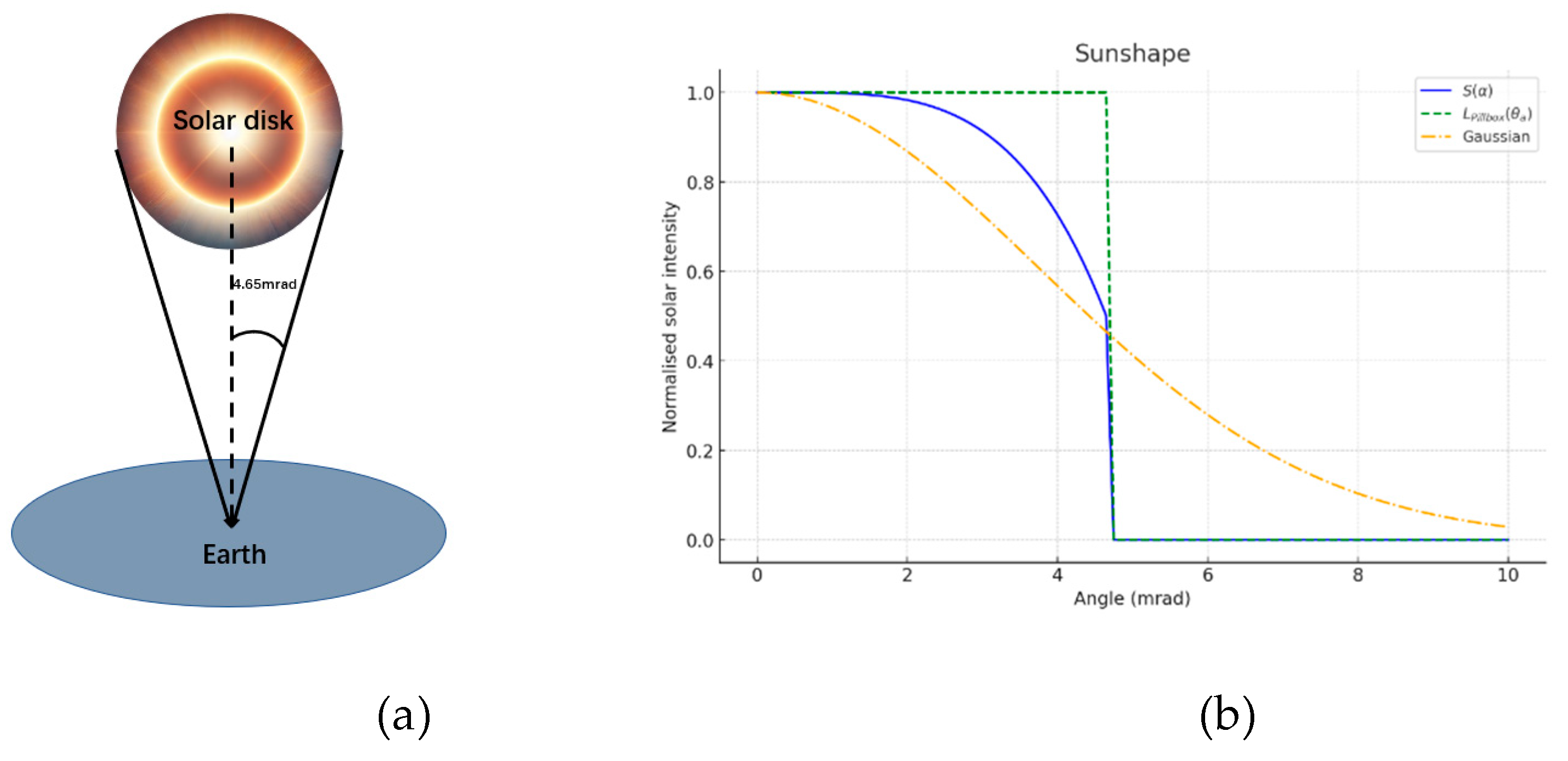
Figure 2.
Illustration of coordinate systems.
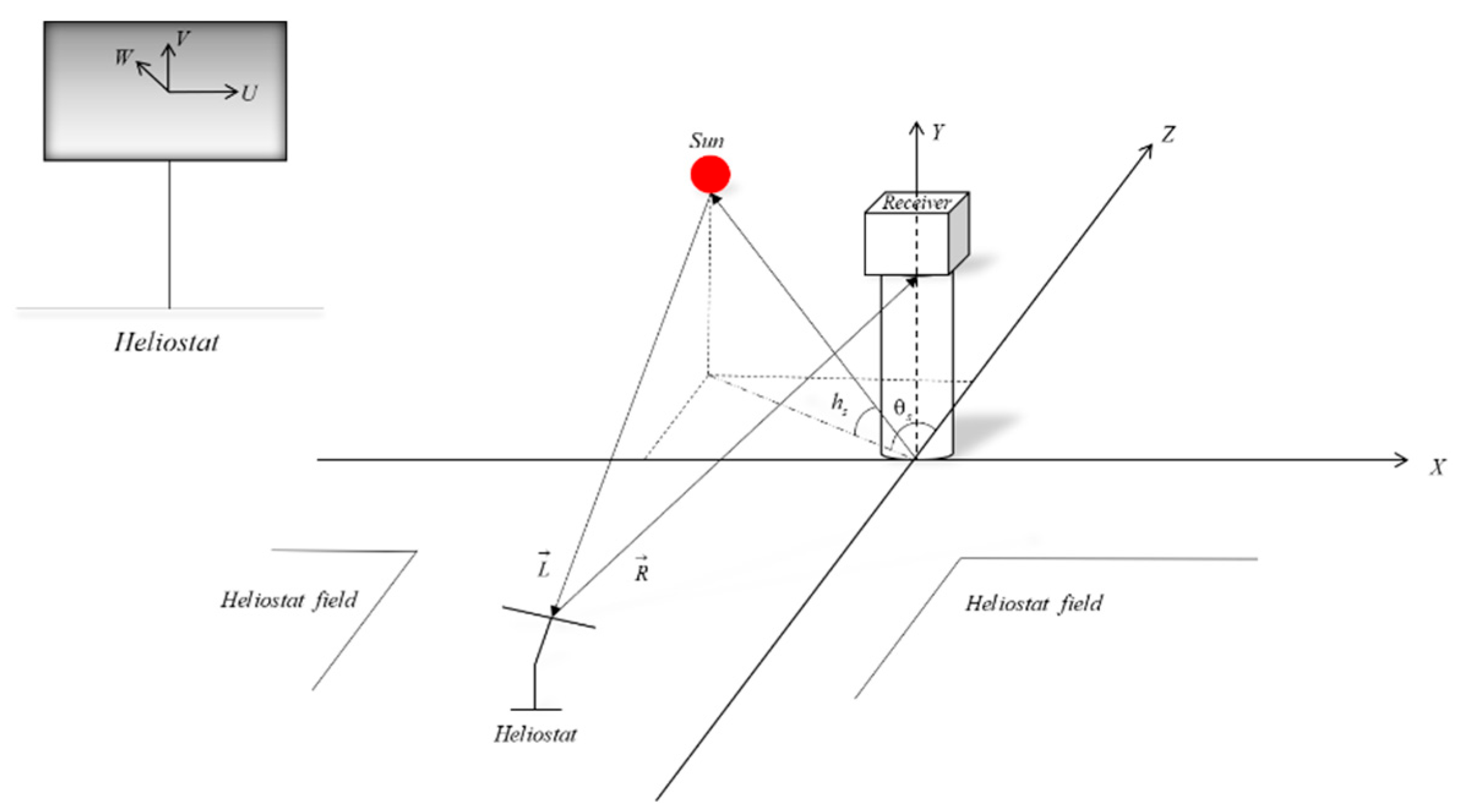
Figure 3.
Non-parallel incident light ray vector representation
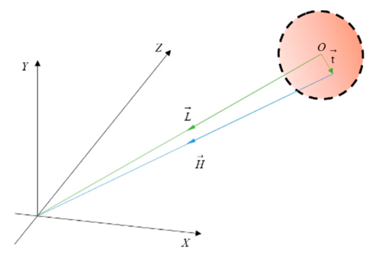
Figure 4.
Side and top views of the heliostat.
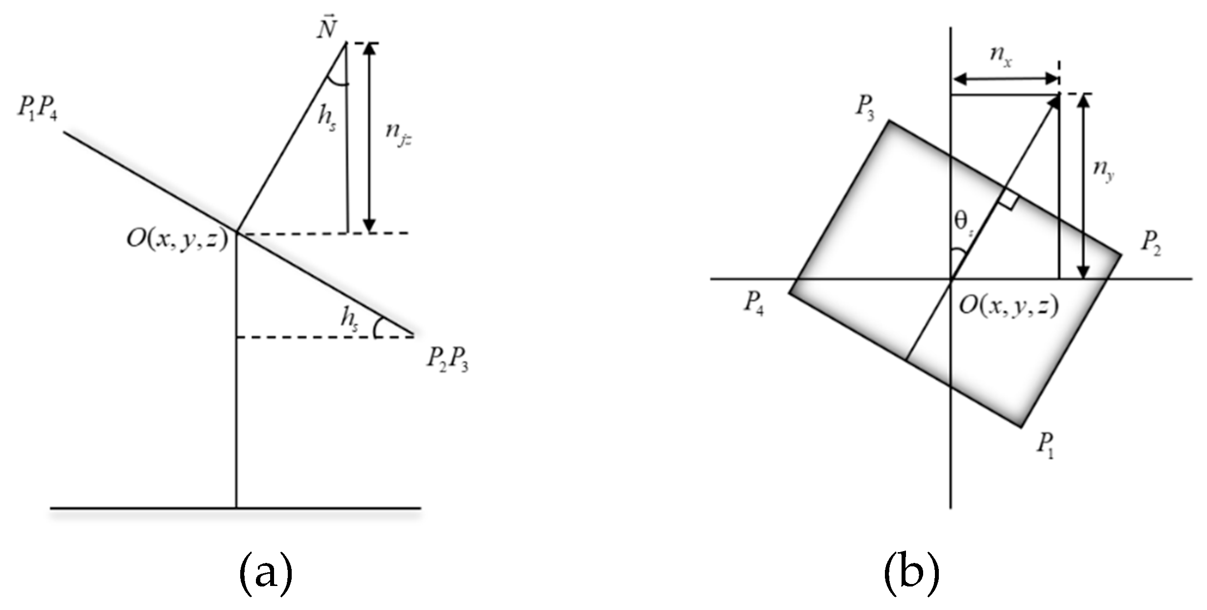
Figure 5.
Schematic diagram of incident and reflected ray unit vector calculation.
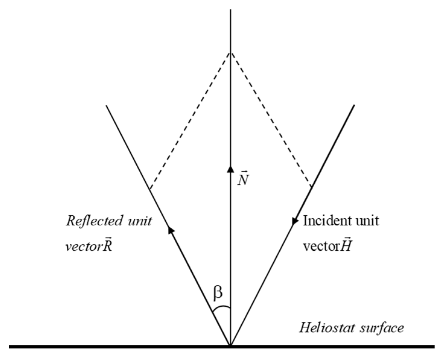
Figure 6.
Framework of Pix2Pix.
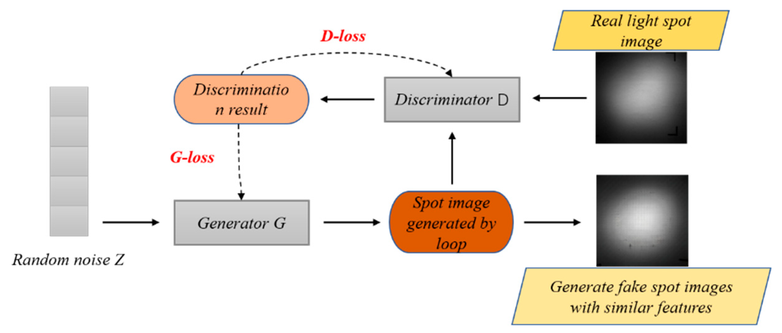
Figure 7.
The structure of U-net.
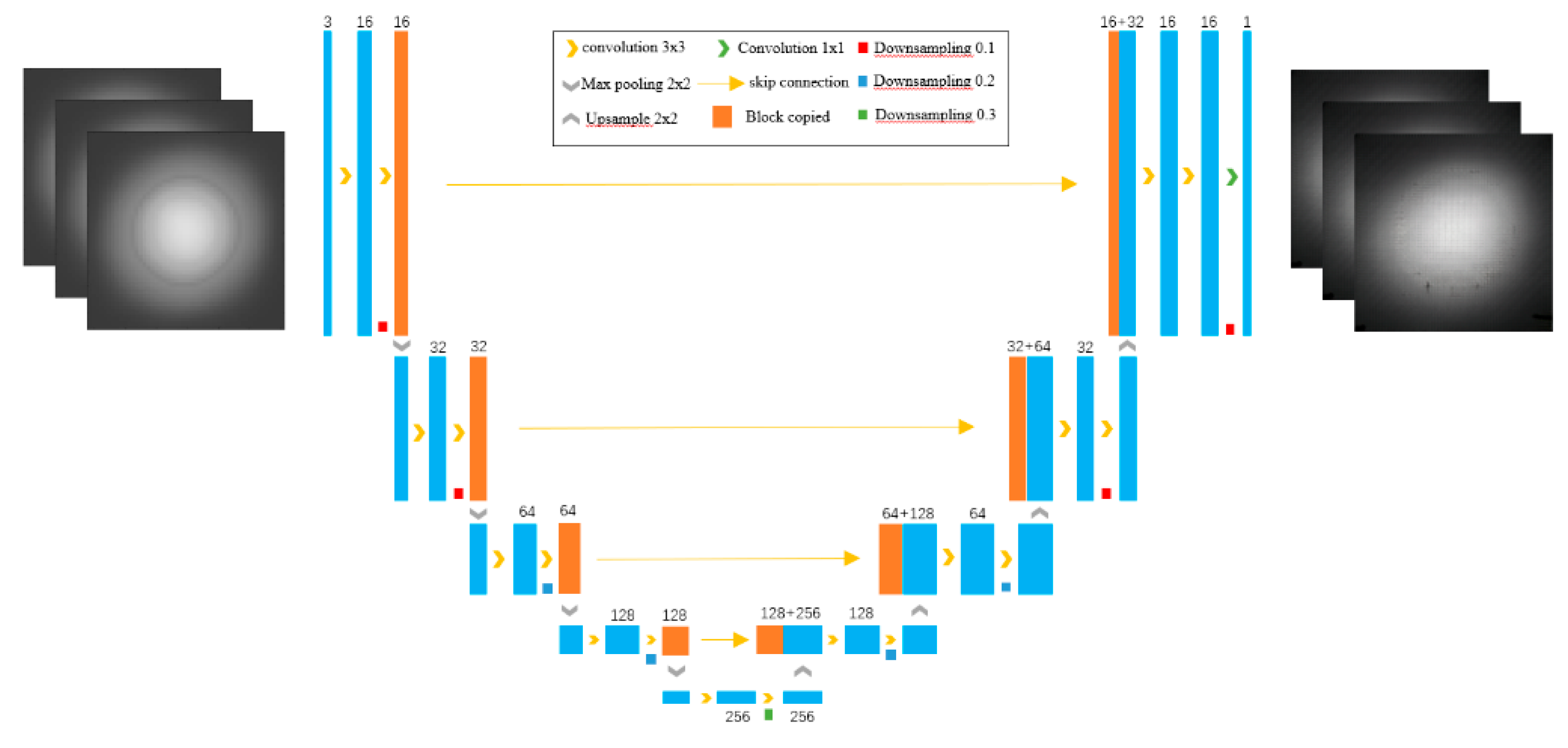
Figure 8.
Schematic diagram of PatchGAN.
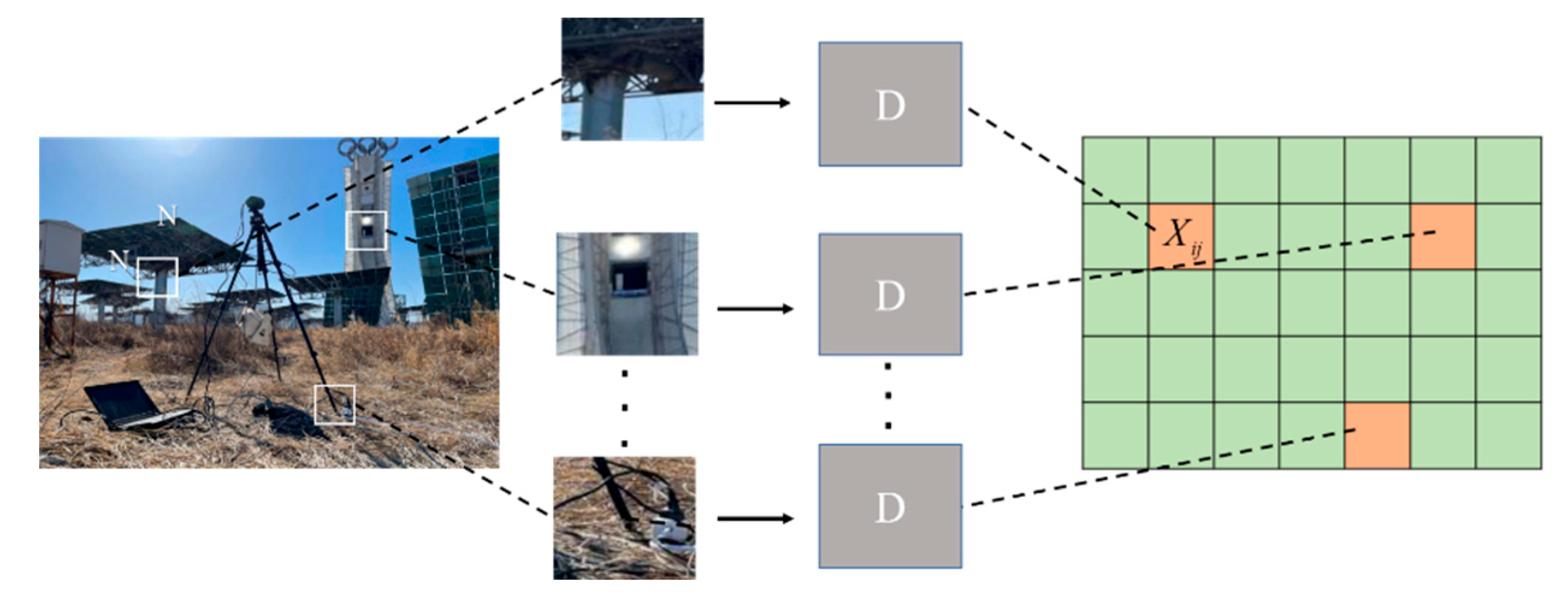
Figure 9.
Example of images generated with different methods.
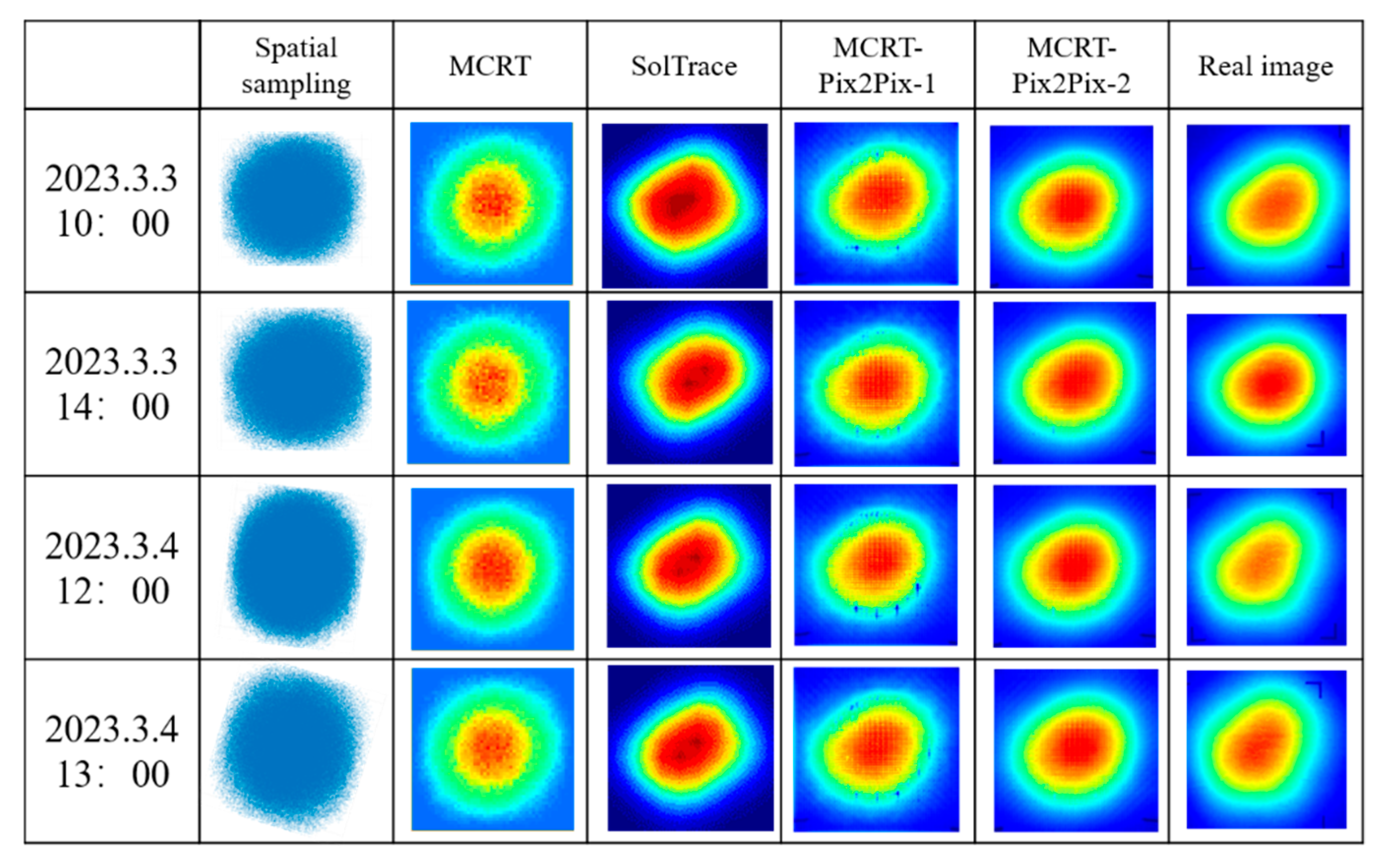
Figure 10.
SSIM values of samples.
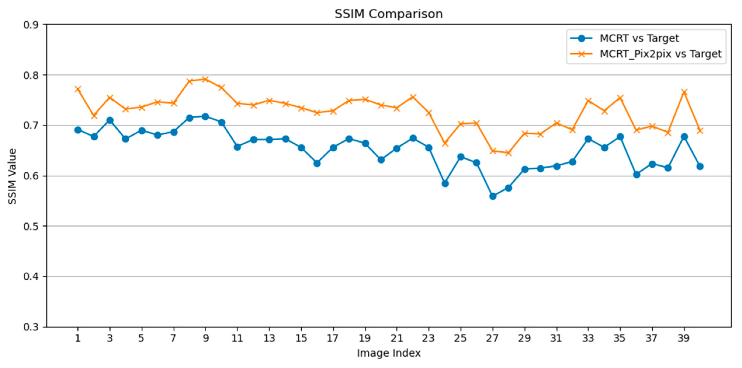
Figure 11.
Cosine similarities in the spatial domain for 50 test samples.
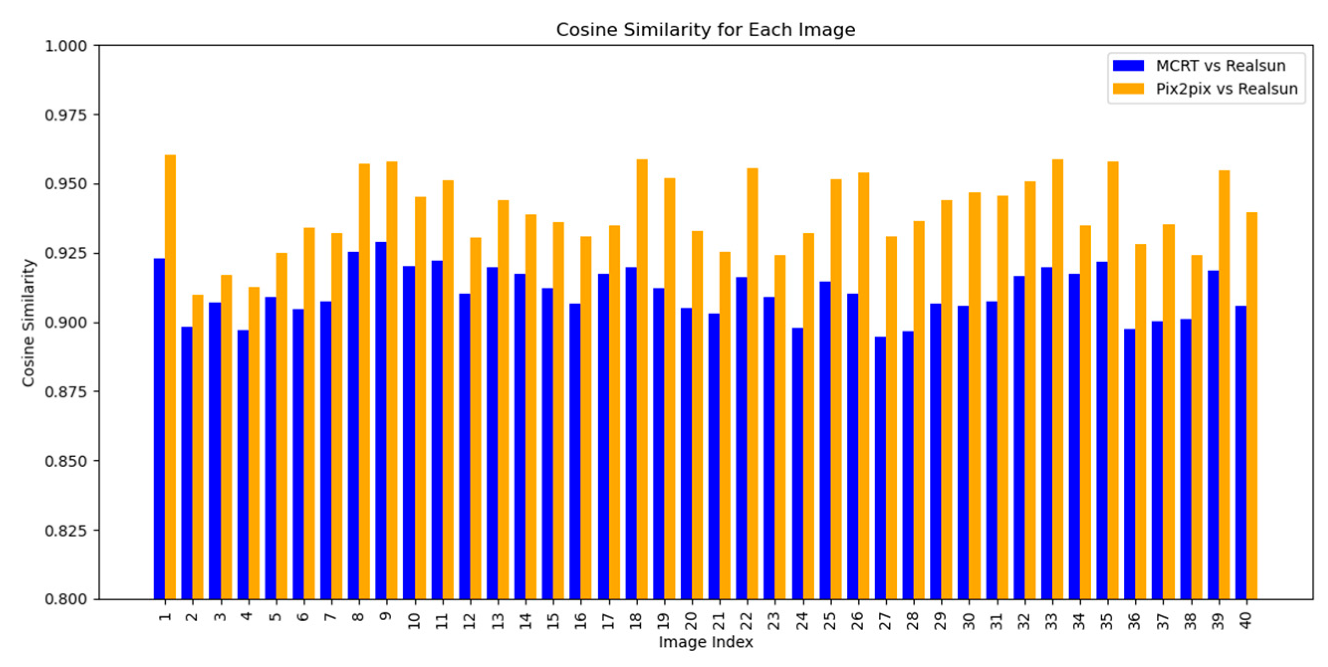
Figure 12.
(a) Comparison of cosine similarity of the spectrum (b) Comparison of cosine similarity of the central part of the spectrum.
Figure 12.
(a) Comparison of cosine similarity of the spectrum (b) Comparison of cosine similarity of the central part of the spectrum.
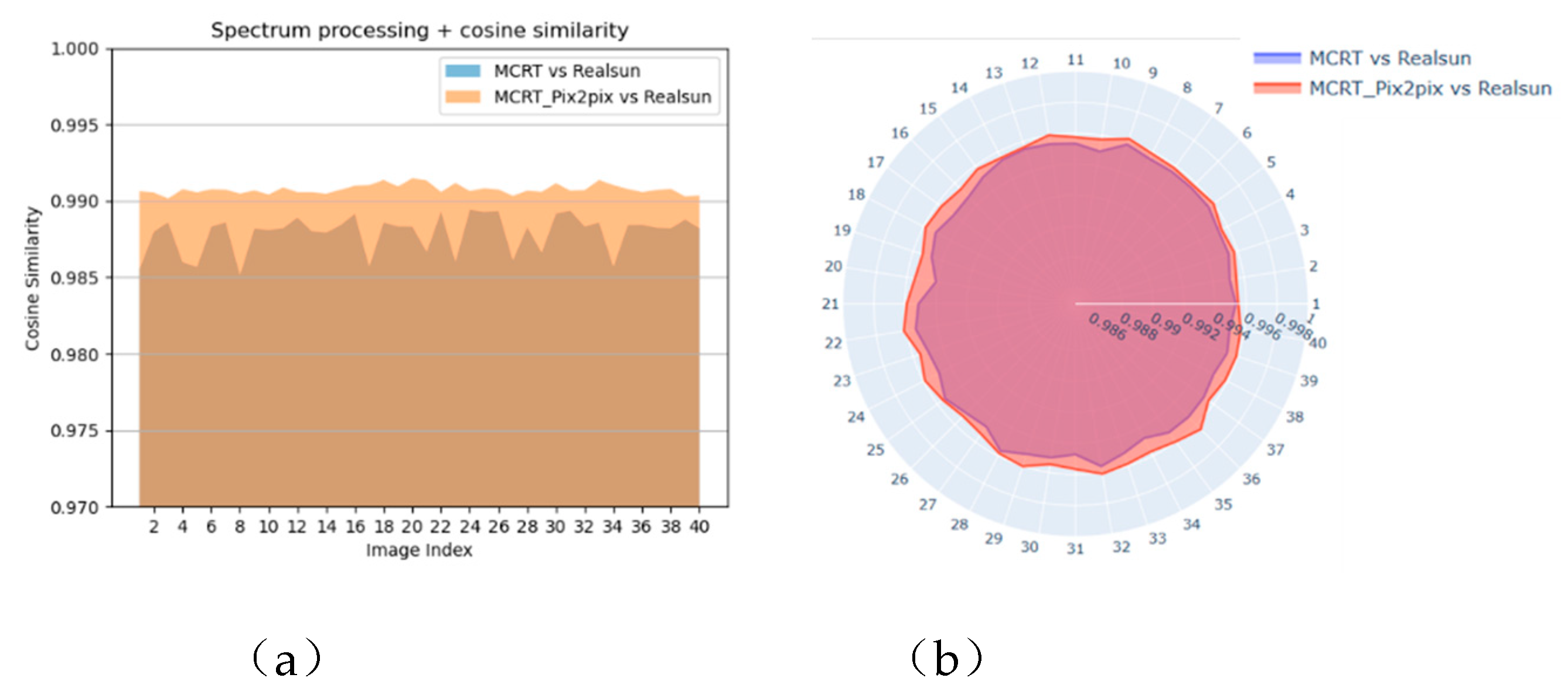
Figure 13.
Comparison of peak signal-to-noise ratio of corresponding light spot images.
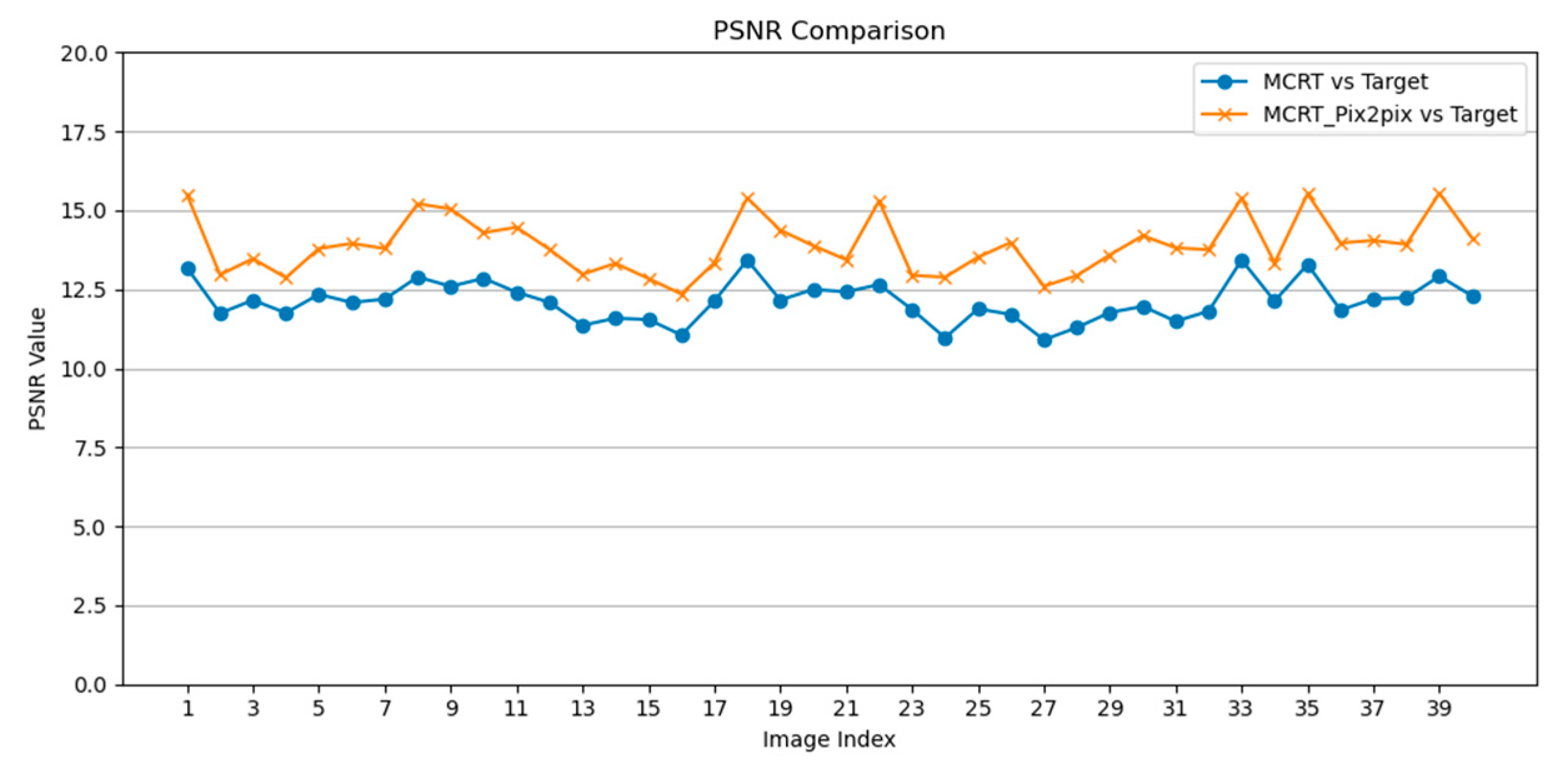

Table 1.
Parameter Settings for ray-tracing Simulation.
| Heliostat field parameters | Simulation values | Heliostat field parameters | Simulation values |
|---|---|---|---|
| Longitude/E | 115.94° | Heliostat size | 10*10 |
| Latitude/N | 40.38° | Heliostat coordinates | (0; 26.7, 5.78) |
| Average altitude/m | 40 | Receiver coordinates | (0; -74; 74.5) |
| Number of mirror light points | 40 million | Receiver size | 5m*5m |
Disclaimer/Publisher’s Note: The statements, opinions and data contained in all publications are solely those of the individual author(s) and contributor(s) and not of MDPI and/or the editor(s). MDPI and/or the editor(s) disclaim responsibility for any injury to people or property resulting from any ideas, methods, instructions or products referred to in the content. |
© 2025 by the authors. Licensee MDPI, Basel, Switzerland. This article is an open access article distributed under the terms and conditions of the Creative Commons Attribution (CC BY) license (http://creativecommons.org/licenses/by/4.0/).
Copyright: This open access article is published under a Creative Commons CC BY 4.0 license, which permit the free download, distribution, and reuse, provided that the author and preprint are cited in any reuse.


