
Submitted:
28 February 2025
Posted:
03 March 2025
You are already at the latest version
Abstract
Fatigue-induced crack initiation and propagation is a major concern in pearlitic railway rails and wheels. Rails and wheels undergo significant plastic deformation on their surface-near layers during service, leading to the initiation and propagation of cracks within the deformed region. Existing models typically use finite element models (FEM) to describe these kind of fatigue phenomena. However, they fail to establish a strong connection between the microstructure of the undeformed and the deformed materials and their corresponding fatigue properties. Therefore, we developed a model based on the soft-contact Discrete Element Method (DEM) that considers microstructural details such as prior austenite grains (PAG), pearlite blocks, pearlite colonies, and lamellar orientation of the ferrite-cementite structure of the pearlite. The Voronoi Tessellation method was used to generate a hierarchical mesh to represent these microstructural details, considering the distribution of microstructural details. The crack propagation is simulated by applying damage laws on the microstructural interface level that degrades the stiffness of the fibers connecting the mesh elements. The model's crack growth predictions are compared to experimental results from the literature to validate its accuracy for different deformation degrees.
Keywords:
Fatigue crack growth
; Discrete element method
; Pearlitic steel
; R260
; Railways
; Voronoi method
1. Introduction
The interaction between the wheel and rail significantly impacts railway performance and safety. The contact forces at the wheel-rail interface support the vehicle's weight, acceleration, braking, and steering forces [1]. If stresses in the contact areas are greater than the plastic yield limit, the material experiences plastic deformation. Pearlitic steel is the common material used in manufacturing rails and wheels in Europe [1]. The mechanical characteristics of pearlitic steel are highly dependent on its microstructural features. For pearlitic steel, the spacing between lamellae is a critical microstructural feature. There is a correlation between the interlamellar spacing and the steel's strength, as demonstrated by Dollar et al. [2]. Bouaziz et al. [3] have also developed a relationship to predict the effect of the interlamellar spacing on the flow stress. Grain size is one of the parameters that can influence the mechanical properties of pearlitic steel. The Hall-Petch relation is one of the most well-known relationships describing grain size's effect on yield strength [4]. Pearlitic steel shows mechanical properties resulting from the mixture of ferrite and cementite, making it strong and resistant to wear without being too brittle; therefore, it can withstand the heavy cyclic loads experienced by railway infrastructure [1].
The contact zone between train wheels and rails is tiny, resulting in high contact pressures that can cause localized severe plastic deformations (SPD) near the surface. Cracks originate mainly from the highly deformed regions below the surface [5]. Improving the crack growth model's reliability and accuracy in SPD regions can increase maintenance planning reliability and traffic safety [6]. Scientists have developed techniques to produce severely deformed microstructures, such as high-pressure torsion (HPT) [7]. The scheme for creating a severely plastically deformed microstructure through the HPT process involves applying substantial torque and hydrostatic pressure to a disk-shaped sample. The usual experimental approach to investigate the effect of severe plastic deformation on the mechanical properties of railway material is to find a relationship between the microstructure, mechanical properties, and the local strain for lab-produced largely deformed microstructure or worn rails [8,9,10,11,12]. The effect of SPD microstructure on fatigue behavior is also widely researched experimentally [13,14,15,16,17,18,19].
Additionally, the effect of plastic deformation on fatigue life was investigated numerically using a parameter that accounts for microstructural characteristics [20,21]. The T-γ model [22] was developed to predict crack initiation using damage function. The finite element method, FEM, combined with cohesive zone modeling, is often used for modeling fatigue crack growth in the literature [23]. Vijay et al. [24] used developed a 3D FEM model to analyze the anisotropy in rolling contact fatigue as a result of anisotropic material properties (randomness) in crystals. Integrating cohesive zone modeling and extended finite element methods enabled Dekker et al. to model crack growth in arbitrary paths [25]. Arata et al. [26] used the cohesive zone modeling method to investigate the crack path within the lamellar structure of titanium aluminide grains. Another alternative approach to model fatigue crack growth is to use the crack growth resistance function in the domain of interest. With the help of such functions, Larijani et al. [27] developed a model to calculate the fatigue crack growth rate anisotropy in near-surface layers of deformed wheel materials without explicitly considering microstructural features. Nezhad et al. [28] developed a 3D finite element model to predict rolling contact fatigue (RCF) crack growth direction and rate in railheads under combined stress and thermal loading.
Other than FEM, some methods are capable of modeling crack growth, such as Discrete Element Method (DEM) and Peridynamic model. DEM is typically used for granular materials. However, it can be employed to model solid-state materials. The discrete element method was first introduced by Cundall and Strack in 1979 to analyze granular material [29]. DEM is a strong computational method for discontinuous material [30,31,32,33,34]. Raje et al. [35,36,37] used the soft contact discrete element model (which is in the family of the DEM) to investigate RCF in roller bearings. Januschewsky et al. [38] developed a DEM model capable of predicting the rolling contact model (RCF) with a novel bond law considering crack closure behavior.
This research presents a method to predict the fatigue crack growth rate (FCG) via DEM in deformed and undeformed microstructures of pearlitic steels. The model is designed to account for the impact of plastic deformation during service life on the microstructure and behavior of cracks. The model employs a hierarchical mesh introduced by Davoodi Jooneghani et al. [39]. In the hierarchsical mesh, each layer represents a distinct microstructural feature. The model combines the DEM and damage criteria. This combination allows for the prediction of the crack growth rate. The influence of plastic deformation on the FCG rate is determined to be substantial, and this outcome is further analyzed by comparing it with crack growth rate data for a particular variant of pearlitic steel, identified as R260, as documented in existing research. The developed model allows us to connect microstructural features with the material's behavior during cyclic loading.
2. Experimental Methods and Materials
The experimental data used for this research was obtained from the studies done on R260 at the Montanuniversität Leoben [18,19,40]. Their experiments include High-Pressure Torsion (HPT) stages and Fatigue Crack Growth (FCG). Their experiment starts with cutting disks from an R260 rod with a 30 mm diameter cut longitudinally from the rail. These 8 mm-thick disks were then sheared via HPT under a pressure of 5.6 GPa, producing two degrees of deformation: 0.25 and 3 rotations. The degree of deformations reached are moderately deformed () and severely deformed (), where is the shear strain. Compact tension (CT) specimens were then machined from these deformed disks according to ASTM 647 standards with orientations as A-T, T-A, R-T, and T-R; which first letter refers to the crack plane normal vector direction, and the second letter shows expected propagation directions relative to the axial (A), tangential (T), and radial directions (R) of the HPT disk [18,19,40]. The shear plane normal vector as the result of deformation is in axial direction. In our study, we focus on A-T and T-A orientations. For FCG testing, the CT specimens undergo further preparation. A fatigue pre-crack is introduced to the specimen using a resonance testing machine. Specimens are subjected to a sinusoidal load with different load ratios (R = 0.1 and 0.7). Crack length is measured using the Potential Drop Technique [18,19,40]. In this research, we selected the load ratio of 0.1.
3. Meshing Methodology
The meshing methodology used in this paper is based on previous research [39]. In general, the 2D representation of the pearlitic steel microstructure is generated by subdividing a domain into cells based on some randomly generated seed points, from which Voronoi polygons are created. These polygons represent the pearlitic steel's microstructural elements like prior austenite grains (PAG), pearlite colonies, and pearlite blocks. To do this, we measured colony, block, and PAG sizes for the undeformed microstructure of R260. Colony size measurements were derived from several scanning electron microscope (SEM) images, with an average colony size of 15 µm. Since blocks are not visible in SEM, Electron Backscatter Diffraction (EBSD) was used for block size analysis, measuring ~ 30 µm. Low-magnification optical microscopy (OM) images provided PAG size measurements similarly, which is calculated to be ~ 60 µm.
The undeformed state, moderately deformed states in the A-T and T-A orientations, and severely deformed states in the A-T and T-A orientations were all represented by meshes created using the mesh methodology outlined in [39]. Three repetitions were made for each of the five deformation states to guarantee model robustness, yielding 20 meshes. These repetitions were similar in the PAG size, pearlite block size, and pearlite colony size as in the original mesh. The only variation among the repetitions was due to the randomness within the hierarchical mesh methodology [39]. These generated meshes were then analyzed for FCG behavior.
A shear strain of 2 was applied for the moderately deformed state. In contrast, a shear strain of 30 was used for the severely deformed (SPD) condition, as these values correspond with data available from Leitner's studies [18,19,40], including data for the undeformed state. The meshes representing different deformation degree microstructures are shown in Figure 2. Their repetitions are not shown here.
Figure 3 shows the angular distribution of lamellae orientations for undeformed, moderately deformed, and severely deformed meshes. The severely deformed microstructure mostly aligns parallel to the shear plane, indicating the highest degree of alignment among the three deformations. However, the moderately deformed microstructure exhibits greater alignment than the undeformed state but less than the severely deformed one.
4. FCG Modeling Using DEM
DEM is an appropriate approach to model fatigue crack growth in undeformed and shear-deformed microstructures because the microstructure can be explicitly considered. A DEM simulation is needed to calculate the stress field around the initial crack in the domain, which ultimately results in fatigue crack growth. The material is modeled in DEM as discrete, rigid entities interacting at their interfaces. Such interactions are modeled with springs, which link the elements together. The springs that join the elements are the only parts that deform; the elements do not deform. A typical two-element DEM setup is illustrated in Figure 4. Two discrete elements, and , are in contact in this setup. The contact between these elements is modeled using springs in normal and tangential directions. The springs in the normal direction control the compressive and tensile interactions, while the tangential springs manage the shear interactions between the elements. Here, and are the stiffness properties in these springs' normal and tangential directions, respectively. When a force is applied to the material, the springs deform according to the relative displacement of the elements they are connected to. The springs' stiffness values in the normal and tangential directions, and , determine how much force is required to produce a given displacement, thereby defining the material's resistance to deformation. The springs' stiffness will degrade as a response to load cycles, following the applied damage law, and eventually, a crack will form.
The springs in a general DEM model can also exhibit damping properties. This damping usually takes the form of damping coefficients that scale with the springs' stiffness. In the current work, damping is not included in the interface formulation. We use this simplification to isolate the measurement of the material's static behavior because only the quasi-static results are of interest for the current study.
The stiffness values in the normal () and tangential () directions in the DEM are derived from integrating the distributed local stiffness along the contact surface length in and . By integrating these local stiffness values over the length of contact (), the global stiffness parameters, and , for the interface are obtained. To derive the governing equilibrium equation in the DEM, we consider two contacting elements, and . When an external load is applied, deformation occurs in the contacting springs between these two elements (see Figure 5). In this figure, represents the center of the contact interface between elements and . is the point located on element at the distance of from . is the point located on element which was in contact with prior to any deformation. Other parameters will be clarified in the following paragraphs.
The normal force and the tangential force can be described as follows in equations (1)-(4), based on Figure 5:
where represents the distributed stiffness of the spring connecting elements and . Furthermore, is the normal component of which describes the fiber stretch connecting two points and in Figure 5. This normal displacement component is used to calculate the normal force generated in the spring, accounting for the stiffness and relative displacement between the elements.
Tangential force resists the sliding motion between the elements like the normal force resists compression or separation. To calculate the tangential force, we have:
where and represent the displacements of the springs at the midpoint of the contact face in the normal and tangential directions for element , which is in contact with element . is the rotational stretch of spring at the distance of . and are the rotational displacement at elements and . To proceed, we need to relate and to the displacement of the center point of elements. Displacement of the center point of elements and are:
, , are displacements in global coordinates in the and directions and rotational displacement of element.
Displacements of the springs at the midpoint of the contact face can be described as:
where is defined as a unit vector perpendicular to the vector connecting the center point of element to the midpoint of the contact face between elements and (see Figure 6). is the component of in direction and is the component of in direction.
To project the displacement vector in normal and tangential directions, we took the following steps:
where is dot product, is the component of a normal vector () in direction and is the component of a normal vector in direction. Similarly, the projection of the displacement vector in tangential directions is done by:
Therefore, we obtain the following expressions for the normal and tangential components of the force:
Given the displacements of the two contacting elements and , the force acting on the surface between these two elements can be calculated. Additionally, momentum (or torque) acting on the surface must be considered. The momentum should be calculated around the center point of the element. The momentum around the element center point is calculated as follows:
where:
is the momentum resulting from concentrated forces acting on the contacting surface between elements and .
is the momentum resulting from distributed forces acting on the contacting surface between elements and .
is the momentum around the center point of the element.
where is the cross-product and is the lever vector shown in Figure 6. This equation translates the local momentum from the contact face to the element’s center by adding the moment caused by the distance between the two points. Therefore, the can be expressed as:
In equation (14), , , and are the stretch of the spring due to displacement in normal, tangential, and rotational direction. By expanding equation (14), we obtain:
Until now, we calculated the forces and the momentum acting on element due to contacting element . However, in our meshes, elements have contact with several other elements. The other contacting elements are as , , ……, and assuming element has contact with other elements. To achieve equilibrium for element , the sum of all forces and moments due to contacts with each neighboring element must be balanced. Therefore, for the equilibrium of the element in global , and rotational direction, we have:
In equations (16)-(18), the contacting elements (, , ……, and ) should be known. To improve efficiency, a faster method [36] is employed by restricting the search region to the immediate vicinity of the element. The details of this method are mentioned in the Figure 7.
To solve equations (16), (17), and (18) for a mesh containing elements, we can rewrite them in a more generalized matrix form, which will help facilitate the solution process. As mentioned earlier, we have already identified the contacting elements (, , ……, and ) for element . For a system with elements, these equations can be expressed as:
In -direction:
In -direction:
In -direction:
, , and () are calculated from the expansion of equations considering all the contacting elements. To solve equations (19), (20), and (21), we organized them like a stiffness matrix in equilibrium analysis. Just like in a traditional stiffness matrix formulation, where the relationship between forces and displacements is represented through a global matrix equation, we can describe the equilibrium of forces and moments acting on an element as:
where, is the stiffness matrix that incorporates the interaction between all contacting elements. This matrix would include contributions from the neighboring elements (, , ……, and ) in contact with element . The vector represents the unknown displacements, and represents the forces acting on the elements due to the forces at the boundaries of the mesh domain. If we expand the matrix and assume there are no boundary forces, the equation can be expressed in its expanded form as follows:
Normal and tangential stiffness calibration directly impacts stress and strain calculation. As a result, many studies have focused on calibrating these stiffnesses to enhance the prediction of stress and strain for different materials in DEM. Following the findings of Raje et al. [36], we selected the stiffness values as detailed below in equations (24) and (25). In this context, represents the distance between the centers of elements i and j, projected along the normal direction and, is the thickness of the elements, is the elastic modulus and is the Poisson's ratio.
The stress near the initial crack is calculated in the model by applying a force on the domain's boundary. The magnitude of the applied force is determined based on available data from the literature, which is in the form of stress intensity factors. Linear elastic fracture mechanics principles convert stress intensity factors into the boundary forces. The corresponding boundary forces were calculated to match the stress intensity factor values reported in the literature. Then, based on the damage law proposed by Raje et al. [36], the springs' stiffness will degrade as a response to load cycles, leading to crack propagation from the initial crack. A damage parameter D is defined and assigned to each interface. Initially, D is set to zero and gradually increases to a maximum value of 1 as load cycles progress.
where and are the initial stiffness in normal and tangential directions.
The damage parameter must increase with load cycles and the amplitude of applied stresses at the interface. For a damage law suitable for the proposed meshing methodology, it is essential to account for the multi-layered mesh structure. Since crack growth behavior differs based on whether it grows along or breaks through cementite lamellae, two distinct conditions are proposed: one for when the crack propagates along the cementite layers and another for when it penetrates through them (see Figure 8).
When a crack grows alongside the cementite and ferrite interface, as shown in Figure 8 (a), the following power-law relation is proposed for the rate of damage evolution in an interface. This relation combines the ideas and approaches of the Peridynamic fatigue cracking model of Silling and Askari [42] and the fatigue threshold model of Lucas and Gerberich [43].
In this context, represents the damage evolution at the interface due to the normal stress acting on it. Here, is the material’s yield stress, is constant, is the length of the contacting interface, while is the threshold stress below which the crack does not propagate. The stress of the threshold may also depend on other material properties. Similarly, we can define the damage evolution when the stress is tangential to the interface of ferrite and cementite interface (damage because of tangential stress ()).
Equation (28) and (29) apply when the crack propagates along the interface between cementite and ferrite. However, when the crack breaks through the cementite lamellae, it must overcome stress greater than due to the higher strength of the cementite. In this scenario, the crack must surpass critical stress (characteristic strength of cementite ()), representing the strength required to fracture the cementite, typically exceeding the yield stress. For this case, we have the following equations governing the damage evolution under normal and tangential loading conditions:
Thus, after calculating the separate damage evolutions for normal and tangential loads, the overall damage evolution can be determined as follows:
.
It is worth noting that for other interfaces within the mesh, such as block, colony, and PAG boundaries, equations (28) and (29) are used because crack propagating through these interfaces does not require cementite breakage.
Once damage parameter reaches a value of 1, a crack propagates along the interface, requiring multiple load cycles. Simulating each load cycle, however, is computationally time-consuming. Therefore, the Jump-In-Cycles method, described by [36], is used to model fatigue damage. This method applies a small increment, , to the damage variable for each cycle block, , while keeping the stress level constant (Figure 9).
When the desired crack length is reached by degrading several interfaces, we calculate the average slope of crack length versus the load cycles graph. This slope represents the crack growth rate under the specific load value related to the applied stress or stress intensity factor. This procedure is repeated for multiple data points (different load values), and each crack growth rate is used in the fatigue crack growth (FCG) graph. The structure of the calculation is shown in detail in Figure 10. As previously described and shown in this figure, the boundary stresses in the simulation () are chosen based on the target stress intensity factors using Linear Elastic Fracture Mechanics (LEFM). A crack growth simulation is done for each selected boundary stress (data point) until the desired crack length is reached. The crack growth rate for each data point is then recorded. By repeating the procedure for data points, the final fatigue crack growth rate diagram can be plotted.
5. Results and Discussion
The meshes described in Figure 2 and their repetitions were used in the DEM model. For the simulation process, damage model parameters must be chosen for each level of deformation. The damage model explained in equations (28)-(32) was calibrated to match the undeformed state and tested and validated for both moderately deformed and severely deformed states. For determining the yield stress, , in the damage model, the research by Tomlison et al. [44] was used. In their study, they modeled the yield stress as a function of the shear strain () using the equation (33) for R260:
By using equation (33), we can calculate the yield stress for the undeformed state to be , for moderately deformed () to , and for severely deformed () to . The threshold stress () can be derived proportional to the stress intensity factor threshold () with the help of previously mentioned linear elastic fracture mechanics (LEFM). The values for for different deformation states are for undeformed, for moderately deformed (), and for severely deformed () based on the experiments done by Leitner et al. [18,19,40]. The characteristic strength of cementite () is approximately based on the research conducted by Garvik et al. [45]. and in equations (28)-(32) were fitted for the undeformed state (see Figure 11) to be and and used to validate other deformation degrees. The results exhibit scattering, as the range shown by the error bars in Figure 11. This scattering is likely due to inherent randomness in the model.
The result of fatigue crack simulation and the experimental results for different deformation states are shown in Figure 12. To generate Figure 12, all four repetitions of three deformation state meshes needed to be run, and the combined result with the error bar was calculated and shown in this figure. It is worth emphasizing again that these results are parameterized for the undeformed state and validated for both deformed and severely deformed states. Measurement errors or unaccounted parameters may cause a difference in the FCG rate for the severely deformed state between simulation and experiments. However, the results are sufficiently acceptable because the same damage law and constant parameters were used throughout the analysis.
Another interesting set of results that can be concluded from the DEM simulation is the crack paths for each deformation state. The crack path for the meshes is shown in Figure 13. The results show that when the deformation goes higher, the crack path tends to be smoother, which is in agreement with the observation reported by Leitner et al. [18,19,40].
As shown in Figure 13, the degree of deformation and its orientation significantly influence the crack trajectory. The model predicts that cracks primarily grow along the interface between cementite and ferrite lamellae when there are no geometrical constraints. This prediction is consistent with the findings of Leitner et al. [40], which state that in pearlitic steels, cracks predominantly propagate along the interface between the ferritic and carbon-rich (previously cementite) phase. Crack tortuosity is a parameter that can describe how twisted or curved a crack path is compared to a straight-line crack path. Crack tortuosity parameter measures the deviation of a crack path from a perfectly straight path. It is defined as the ratio of the actual path to the straight-line distance between the crack's beginning and end (In this case, the distance along the x-coordinate). Figure 14 shows the crack tortuosity for different deformation states simulated by DEM. It is important to note that tortuosity was not calculated for the severely deformed state in the T-A orientation because of the extremely short crack length along the x-coordinate; this value would be much higher than others. The higher values of crack tortuosity may explain the crack growth rate anisotropy in pearlitic rail steel material. For slower orientation, e.g., T-A orientation, the crack should encounter more deviation in its path when it needs to reach a specific length.
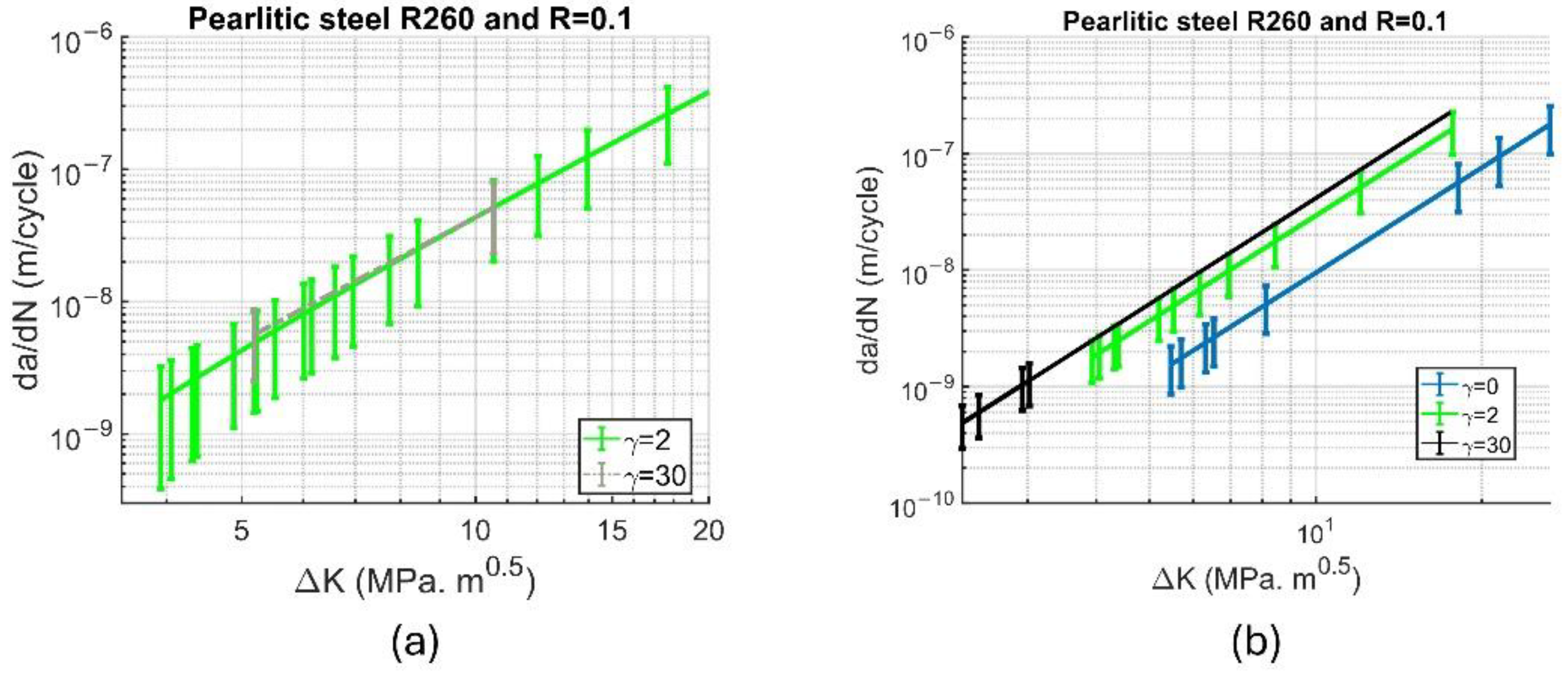
To investigate the influence of the different deformation states on fatigue resistance, we simulated the crack evolution of SPD and moderately deformed meshes under similar stress intensity factor ranges. The results shown in Figure 15. (a) were obtained with the previously adjusted values of and . Figure 15. (a) show that the differences in the FCG rate between the SPD and moderately deformed conditions are minimal. This means that the increment in the FCG rate predicted by the model starts already at moderate deformation level of (see comparison with undeformed state in Figure 12). Furthermore, simulations were performed using same values of and to isolate the effect of mesh deformation on FCG (see Figure 15. (b). The results show that the FCG rate increases mainly due to re-orientation of microstructural components occurring already at moderate deformation of . Finally, we can conclude that the strain hardening that modifies the yield strength does not considerably affect the FCG rate.
6. Summary and Conclusions
This paper presents a methodology to predict the relation of microstructural parameters to the fatigue crack growth behavior in plastically deformed pearlitic steel using DEM and hierarchical meshing methods presented in an earlier work [39]. This meshing methodology enabled us to model complex meshes representing various microstructural features of the pearlitic steel. Plastic deformation was also considered in the mesh via simple geometrical shearing. Several meshes were generated and analyzed using the DEM model to investigate the crack growth and the effect of plastic deformation. The model can capture the fatigue crack growth rate anisotropy induced in the material due to the deformation.
From this work we can conclude that:
- The crack grows faster in deformed pearlite as in undeformed microstructure due to the orientation of the microstructural features
- The crack growth rate slightly decreases with the strain hardening from the plastic deformation (yield strength)
- The reorientation of the pearlite lamellae results in lower tortuosity in SPD conditions compared to the undeformed condition. The lower tortuosity leads to higher FCG rate
The model can correlate the plastic deformation with the microstructural features and the fatigue properties to estimate the RCF lifetime of wheel-rail material. Finally, the reasons for slight deviations between measurements and modelled results can be that the models do not account for plasticity, breakage or dissolution of the cementite, and that the damage model is simple.
Author Contributions
Conceptualization, H.D.J. and K.S. and M.C.P. and G.T.; methodology, H.D.J. and S.S.Sh. and K.S. and M.C.P. and G.T.; software, H.D.J. and S.S.Sh. and K.S. and M.C.P. and G.T.; validation, H.D.J. and S.S.Sh. and K.S. and M.C.P. and G.T.; formal analysis, H.D.J. and S.S.Sh. and K.S. and M.C.P. and G.T.; investigation, H.D.J. and S.S.Sh. and K.S. and M.C.P. and G.T.; writing—original draft preparation, H.D.J.; writing—review and editing, H.D.J. and S.S.Sh. and K.S. and M.C.P. and G.T.; visualization, H.D.J. and S.S.Sh. and K.S. and M.C.P. and G.T.; supervision, K.S. and M.C.P. and G.T.; project administration K.S. and M.C.P. and G.T.; funding acquisition, G.T. All authors have read and agreed to the published version of the manuscript.
Funding
This research was funded in whole, or in part, by the Austrian Science Fund (FWF) under project No. P 34612-N. The publication was partly written at Virtual Vehicle Research GmbH in Graz and partially funded within the COMET K2 Competence Centers for Excellent Technologies from the Austrian Federal Ministry for Climate Action (BMK), the Austrian Federal Ministry for Labour and Economy (BMAW), the Province of Styria (Dept. 12) and the Styrian Business Promotion Agency (SFG). The Austrian Research Promotion Agency (FFG) has been authorized for programme management. For the purpose of open access, the author has applied a CC BY public copyright license to any Author Accepted Manuscript version arising from this submission.
Data Availability Statement
Data will be available upon request.
Conflicts of Interest
The authors declare no conflicts of interest.
Appendix A
The Model parameters used in the simulation are summarized in Table A1.

Table A1.
Model parameters used in the fatigue crack growth simulation.
| Variable | Description | Value [Unit] |
|---|---|---|
| [-] | ||
| [-] | ||
| ] | ||
References
- Olofsson, U. Wheel-rail interface handbook. 2009.
- Dollar, M.; Bernstein, I.; Thompson, A. Influence of deformation substructure on flow and fracture of fully pearlitic steel. Acta Met. 1988, 36, 311–320. [Google Scholar] [CrossRef]
- Bouaziz, O.; Le Corre, C. Flow Stress and Microstructure Modelling of Ferrite-Pearlite Steels during Cold Rolling. Mater. Sci. Forum 2003, 426-432, 1399–1404. [Google Scholar] [CrossRef]
- Hansen, N. Hall–Petch relation and boundary strengthening. Scr. Mater. 2004, 51, 801–806. [Google Scholar] [CrossRef]
- Cannon, D.; Pradier, H. Rail rolling contact fatigue Research by the European Rail Research Institute. Wear 1996, 191, 1–13. [Google Scholar] [CrossRef]
- Talebi, N.; Ahlström, J.; Ekh, M.; Meyer, K.A. Evaluations and enhancements of fatigue crack initiation criteria for steels subjected to large shear deformations. Int. J. Fatigue 2024, 182. [Google Scholar] [CrossRef]
- Leitner, T. Fatigue Crack Growth of Nanocrystalline and Ultrafine-Grained Metals Processed By Severe Plastic Deformation. Montanuniversitat Leoben, 2017.
- Kumar, A.; Agarwal, G.; Petrov, R.; Goto, S.; Sietsma, J.; Herbig, M. Microstructural evolution of white and brown etching layers in pearlitic rail steels. Acta Mater. 2019, 171, 48–64. [Google Scholar] [CrossRef]
- Kapp, M. Structural instabilities in nanostructured metals. Austrian Academy of Sciences, 2017.
- Masoumi, M.; Ariza, E.A.; Sinatora, A.; Goldenstein, H. Role of crystallographic orientation and grain boundaries in fatigue crack propagation in used pearlitic rail steel. Mater. Sci. Eng. A 2018, 722, 147–155. [Google Scholar] [CrossRef]
- He, Y.; Xiang, S.; Shi, W.; Liu, J.; Ji, X.; Yu, W. Effect of microstructure evolution on anisotropic fracture behaviors of cold drawing pearlitic steels. Mater. Sci. Eng. A 2017, 683, 153–163. [Google Scholar] [CrossRef]
- Hu, Y.; Zhou, L.; Ding, H.; Lewis, R.; Liu, Q.; Guo, J.; Wang, W. Microstructure evolution of railway pearlitic wheel steels under rolling-sliding contact loading. Tribol. Int. 2021, 154. [Google Scholar] [CrossRef]
- Adamczyk-Cieślak, B.; Koralnik, M.; Kuziak, R.; Brynk, T.; Zygmunt, T.; Mizera, J. Low-cycle fatigue behaviour and microstructural evolution of pearlitic and bainitic steels. Mater. Sci. Eng. A 2019, 747, 144–153. [Google Scholar] [CrossRef]
- Meyer, K.A.; Nikas, D.; Ahlström, J. Microstructure and mechanical properties of the running band in a pearlitic rail steel: Comparison between biaxially deformed steel and field samples. Wear 2018, 396, 12–21. [Google Scholar] [CrossRef]
- Dylewski, B.; Risbet, M.; Bouvier, S. The tridimensional gradient of microstructure in worn rails – Experimental characterization of plastic deformation accumulated by RCF. Wear 2017, 392-393, 50–59. [Google Scholar] [CrossRef]
- Rezende, A.; Fonseca, S.; Fernandes, F.; Miranda, R.; Grijalba, F.; Farina, P.; Mei, P. Wear behavior of bainitic and pearlitic microstructures from microalloyed railway wheel steel. Wear 2020, 456-457, 203377. [Google Scholar] [CrossRef]
- Stock, R. Influencing rolling contact fatigue and wear by different rail grades and contact conditions. 2011.
- Leitner, T.; Hohenwarter, A.; Pippan, R. Anisotropy in fracture and fatigue resistance of pearlitic steels and its effect on the crack path. Int. J. Fatigue 2019, 124, 528–536. [Google Scholar] [CrossRef]
- Leitner, T.; Trummer, G.; Pippan, R.; Hohenwarter, A. Influence of severe plastic deformation and specimen orientation on the fatigue crack propagation behavior of a pearlitic steel. Mater. Sci. Eng. A 2018, 710, 260–270. [Google Scholar] [CrossRef]
- McDowell, D.L. Simulation-based strategies for microstructure-sensitive fatigue modeling. Mater. Sci. Eng. A 2007, 468-470, 4–14. [Google Scholar] [CrossRef]
- Przybyla, C.; Prasannavenkatesan, R.; Salajegheh, N.; McDowell, D.L. Microstructure-sensitive modeling of high cycle fatigue. Int. J. Fatigue 2010, 32, 512–525. [Google Scholar] [CrossRef]
- Evans, J.R.; Burstow, M.C. Vehicle/track interaction and rolling contact fatigue in rails in the UK. Veh. Syst. Dyn. 2006, 44, 708–717. [Google Scholar] [CrossRef]
- Park, K.; Paulino, G.H. Cohesive Zone Models: A Critical Review of Traction-Separation Relationships Across Fracture Surfaces. Appl. Mech. Rev. 2011, 64, 060802. [Google Scholar] [CrossRef]
- Vijay, A.; Paulson, N.; Sadeghi, F. A 3D finite element modelling of crystalline anisotropy in rolling contact fatigue. Int. J. Fatigue 2018, 106, 92–102. [Google Scholar] [CrossRef]
- Dekker, R.; van der Meer, F.; Maljaars, J.; Sluys, L. A cohesive XFEM model for simulating fatigue crack growth under mixed-mode loading and overloading. Int. J. Numer. Methods Eng. 2019, 118, 561–577. [Google Scholar] [CrossRef]
- Arata, J.; Kumar, K.; Curtin, W.; Needleman, A. Crack growth in lamellar titanium aluminide. Int. J. Fract. 2001, 111, 163–189. [Google Scholar] [CrossRef]
- Larijani, N. Anisotropy in pearlitic steel subjected to rolling contact fatigue - modelling and experiments. 2014.
- Nezhad, M.S.; Larsson, F.; Kabo, E.; Ekberg, A. Finite element analyses of rail head cracks: Predicting direction and rate of rolling contact fatigue crack growth. Eng. Fract. Mech. 2024, 310. [Google Scholar] [CrossRef]
- Cundall, P.A.; Strack, O.D.L. A discrete numerical model for granular assemblies. Géotechnique 1979, 29, 47–65. [Google Scholar] [CrossRef]
- Wittel, F.K.; Kun, F.; Kröplin, B.-H.; Herrmann, H.J. A study of transverse ply cracking using a discrete element method. Comput. Mater. Sci. 2003, 28, 608–619. [Google Scholar] [CrossRef]
- Cheng, M.; Liu, W.; Liu, K. New discrete element models for elastoplastic problems. Acta Mech. Sin. 2009, 25, 629–637. [Google Scholar] [CrossRef]
- Liu, K.; Gao, L.; Tanimura, S. Application of Discrete Element Method in Impact Problems. JSME Int. J. Ser. A 2004, 47, 138–145. [Google Scholar] [CrossRef]
- Kosteski, L.E.; Riera, J.D.; Iturrioz, I.; Singh, R.K.; Kant, T. Analysis of reinforced concrete plates subjected to impact employing the truss-like discrete element method. Fatigue Fract. Eng. Mater. Struct. 2014, 38, 276–289. [Google Scholar] [CrossRef]
- Kosteski, L.E.; Iturrioz, I.; Cisilino, A.P.; D'Ambra, R.B.; Pettarin, V.; Fasce, L.; Frontini, P. A lattice discrete element method to model the falling-weight impact test of PMMA specimens. Int. J. Impact Eng. 2016, 87, 120–131. [Google Scholar] [CrossRef]
- Raje, N.; Sadeghi, F.; Rateick, R.G. A discrete element approach to evaluate stresses due to line loading on an elastic half-space. Comput. Mech. 2006, 40, 513–529. [Google Scholar] [CrossRef]
- Nihar, R. Statistical Numerical Modeling Of Subsurface Initiated Spalling In Bearing Contacts. Purdue University, 2008.
- Raje, N.; Sadeghi, F.; Rateick, R.G. A Statistical Damage Mechanics Model for Subsurface Initiated Spalling in Rolling Contacts. J. Tribol. 2008, 130, 042201. [Google Scholar] [CrossRef]
- Januschewsky, M.; Trummer, G.; Six, K.; Lewis, R. Discrete element modelling of rolling contact fatigue and crack closure with different bond laws. Wear 2024, 544-545. [Google Scholar] [CrossRef]
- Jooneghani, H.D.; Six, K.; Sharifi, S.; Poletti, M.; Trummer, G. Representation of the microstructure of pearlitic steels for DEM simulations of fatigue. Wear 2023, 540-541. [Google Scholar] [CrossRef]
- Leitner, T.; Sackl, S.; Völker, B.; Riedl, H.; Clemens, H.; Pippan, R.; Hohenwarter, A. Crack path identification in a nanostructured pearlitic steel using atom probe tomography. Scr. Mater. 2018, 142, 66–69. [Google Scholar] [CrossRef]
- Raje, N.; Slack, T.; Sadeghi, F. A discrete damage mechanics model for high cycle fatigue in polycrystalline materials subject to rolling contact. Int. J. Fatigue 2009, 31, 346–360. [Google Scholar] [CrossRef]
- Silling, S.; Askari, A. Peridynamic model for fatigue cracks. no. SANDIA REPORT SAND2014-18590, pp. 1–39, 2014.
- Lucas, J.P.; Gerberich, W.W. A PROPOSED CRITERION FOR FATIGUE THRESHOLD: DISLOCATION SUBSTRUCTURE APPROACH. Fatigue Fract. Eng. Mater. Struct. 1983, 6, 271–280. [Google Scholar] [CrossRef]
- Tomlinson, K.; Fletcher, D.; Lewis, R. Measuring material plastic response to cyclic loading in modern rail steels from a minimal number of twin-disc tests. Proc. Inst. Mech. Eng. Part F: J. Rail Rapid Transit 2021, 235, 1203–1213. [Google Scholar] [CrossRef]
- Garvik, N.; Carrez, P.; Cordier, P. First-principles study of the ideal strength of Fe3C cementite. Mater. Sci. Eng. A 2013, 572, 25–29. [Google Scholar] [CrossRef]
Figure 1.
FCG results for undeformed, moderately deformed, and severely deformed microstructure in A-T orientation [18,19,40].
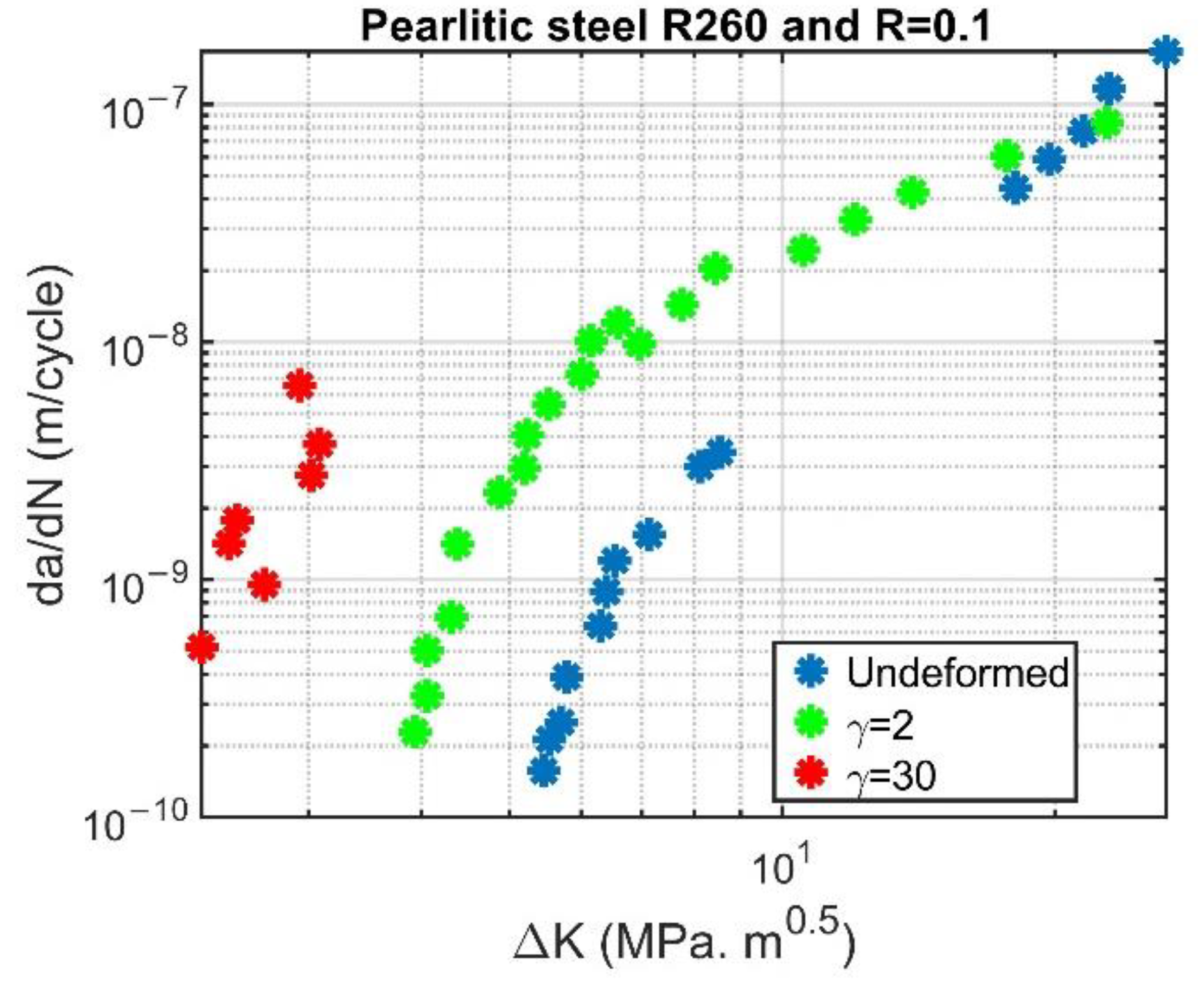
Figure 2.
Meshes representing the state of the R260 microstructure; (a). Undeformed; (b). Moderately deformed; (c). SPD; (d). Moderately deformed in T-A orientation; (e). SPD in T-A orientation.
Figure 2.
Meshes representing the state of the R260 microstructure; (a). Undeformed; (b). Moderately deformed; (c). SPD; (d). Moderately deformed in T-A orientation; (e). SPD in T-A orientation.
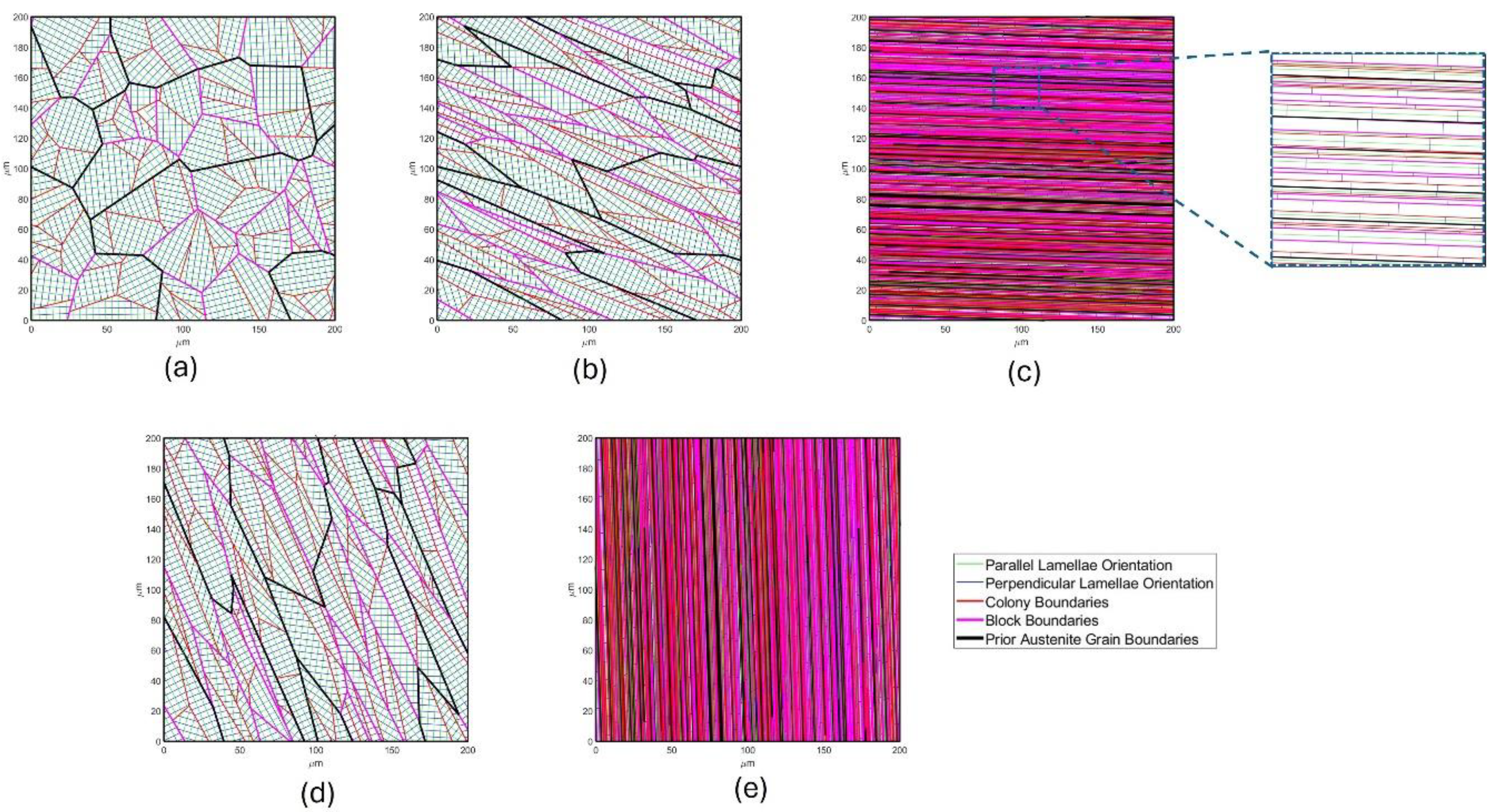
Figure 3.
The angular distribution of lamellae orientations for undeformed (Blue), moderately deformed (Green), and severely deformed microstructures (Red).
Figure 3.
The angular distribution of lamellae orientations for undeformed (Blue), moderately deformed (Green), and severely deformed microstructures (Red).
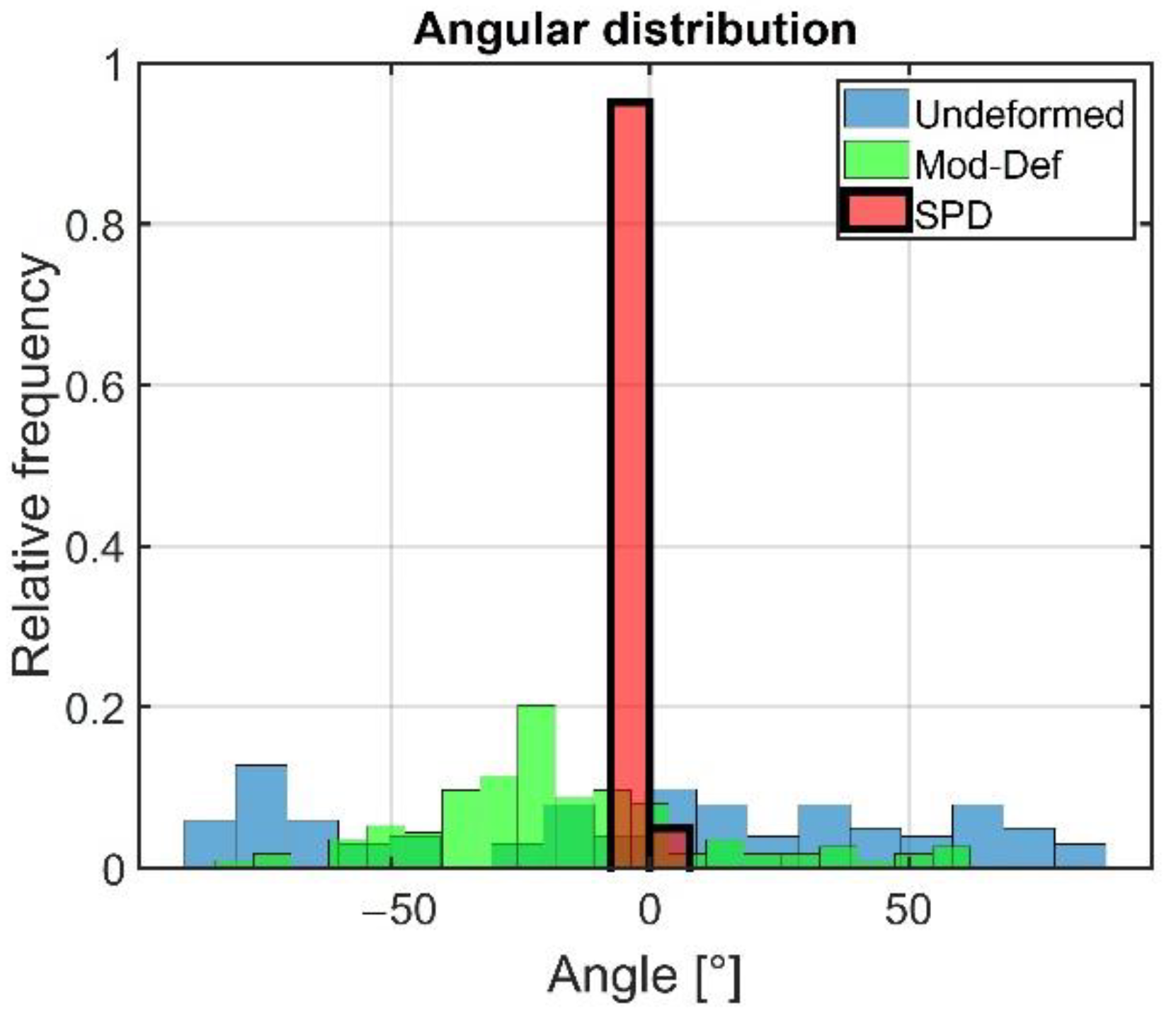
Figure 4.
A typical two-element DEM setup. Image redrawn from [41].
Figure 4.
A typical two-element DEM setup. Image redrawn from [41].
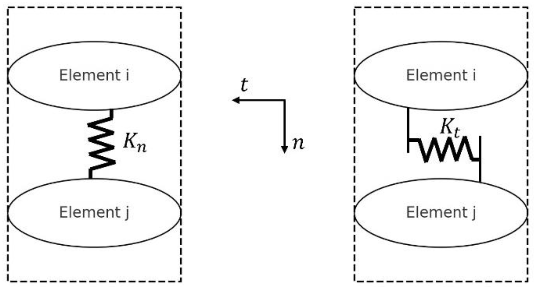
Figure 5.
The normal and tangential displacements of a stretched fiber.
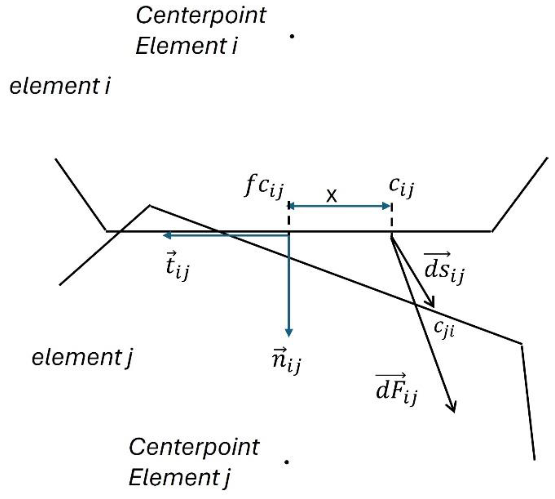
Figure 6.
Definition of and vectors.
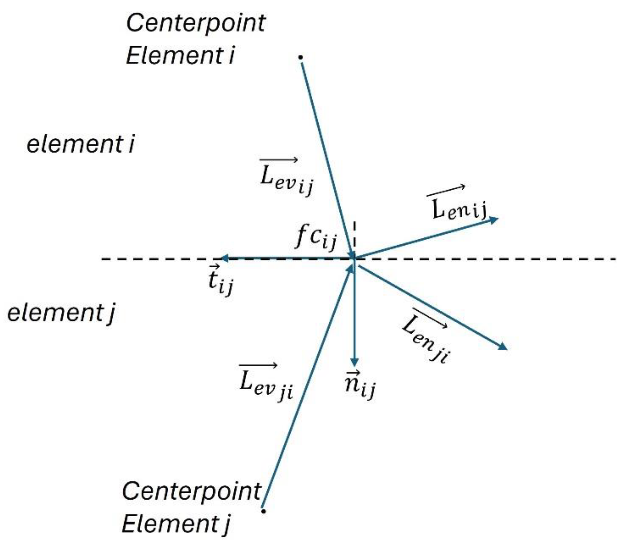
Figure 7.
Contact detection for a home cell with rectangular-shaped elements. Image redrawn from [36].
Figure 7.
Contact detection for a home cell with rectangular-shaped elements. Image redrawn from [36].
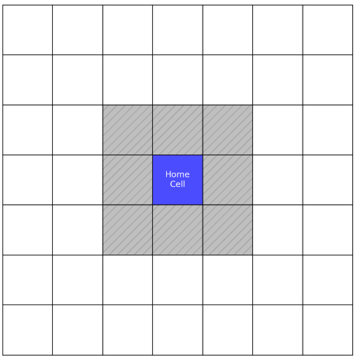
Figure 8.
Crack growth scenario in the mesh. (a) alongside cementite and ferrite interface. (b) through the cementite lamellae (crack breaks the cementite). Red arrows show the direction of crack growth.
Figure 8.
Crack growth scenario in the mesh. (a) alongside cementite and ferrite interface. (b) through the cementite lamellae (crack breaks the cementite). Red arrows show the direction of crack growth.
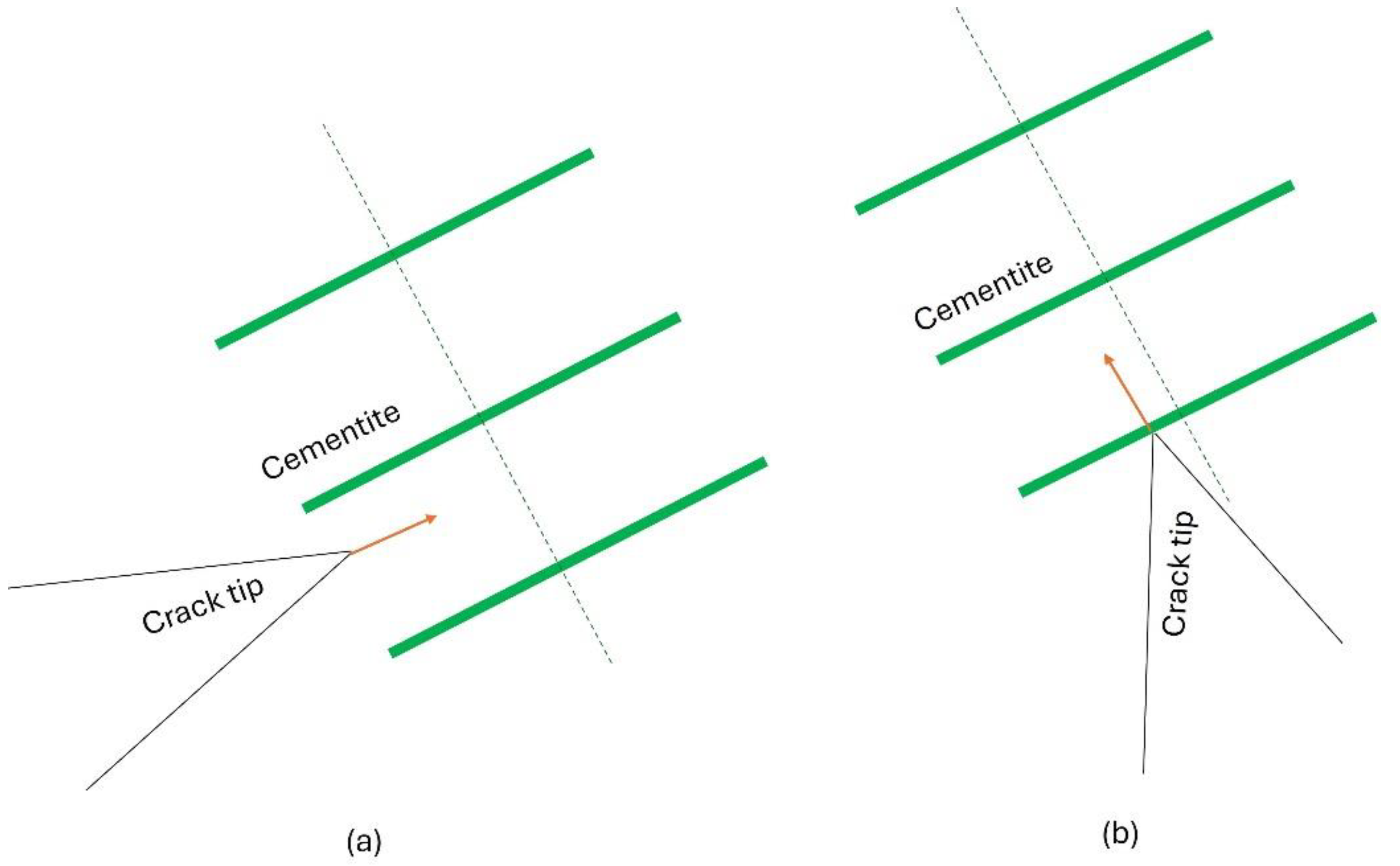
Figure 9.
The Jump-In-Cycles method. Image redrawn from [36].
Figure 9.
The Jump-In-Cycles method. Image redrawn from [36].
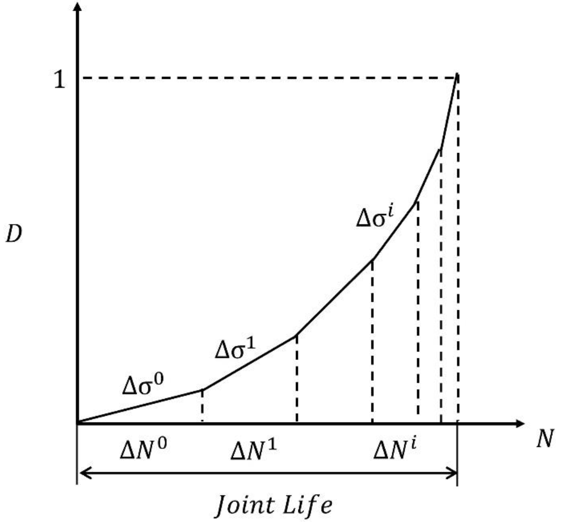
Figure 10.
Algorithm for simulating the fatigue crack growth (FCG) curve using the jump-in-cycles and LEFM methods for estimating stresses.
Figure 10.
Algorithm for simulating the fatigue crack growth (FCG) curve using the jump-in-cycles and LEFM methods for estimating stresses.
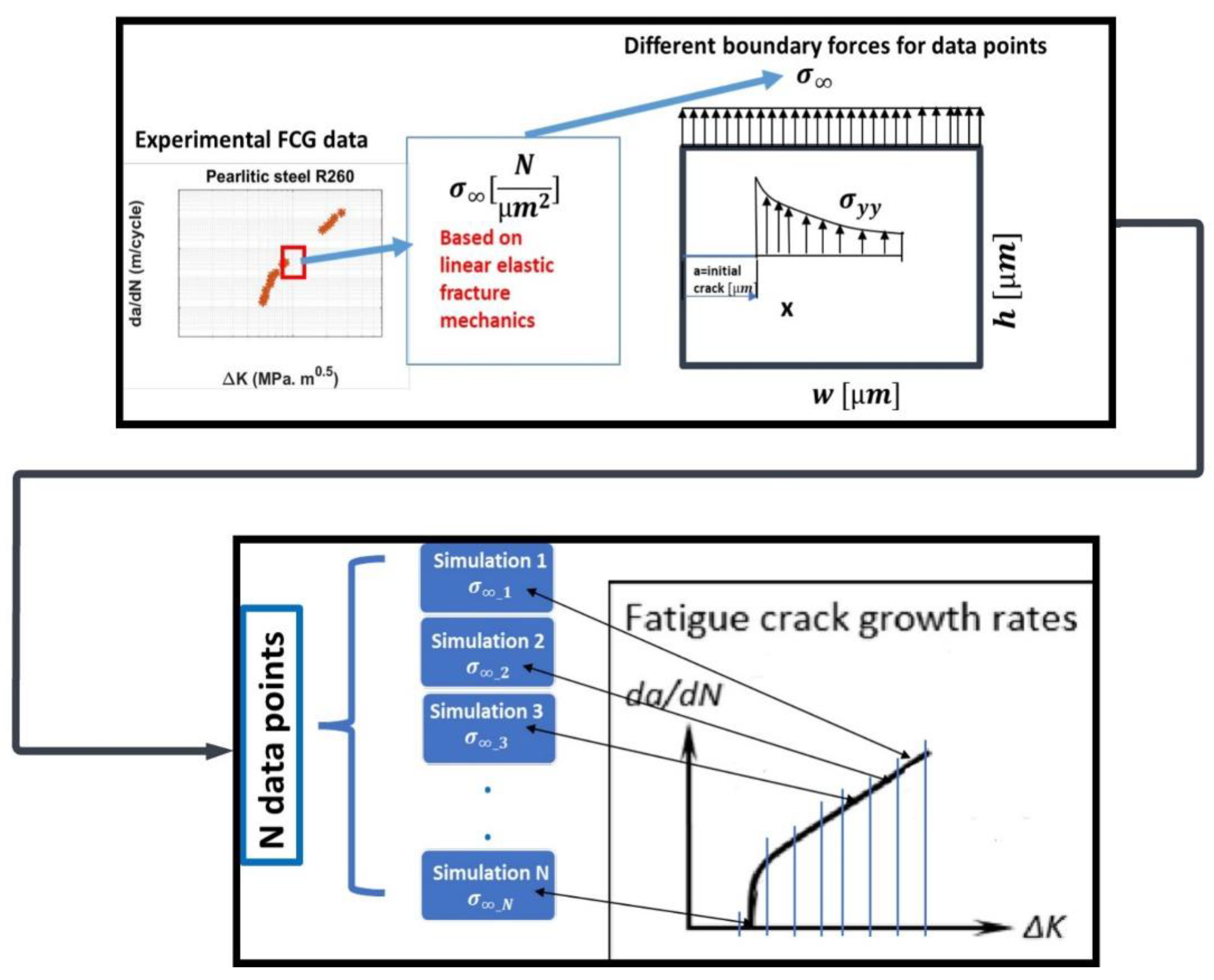
Figure 11.
Fatigue crack growth results for undeformed R260. Stars represent experimental results [18,19,40].
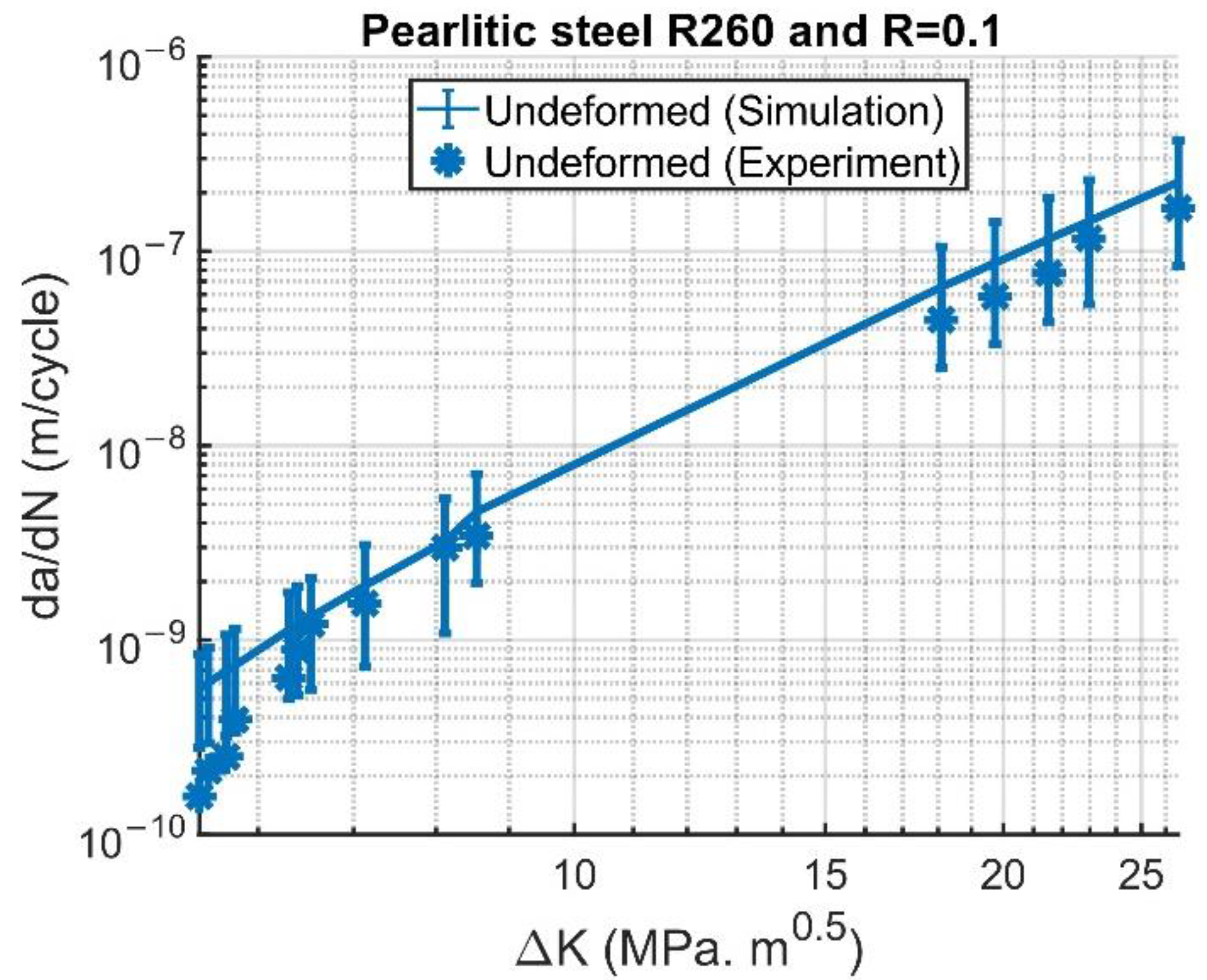
Figure 12.
Fatigue crack growth results in undeformed, moderately deformed, and severely deformed R260. Stars represent experimental results [18,19,40]. The lines are the DEM results.
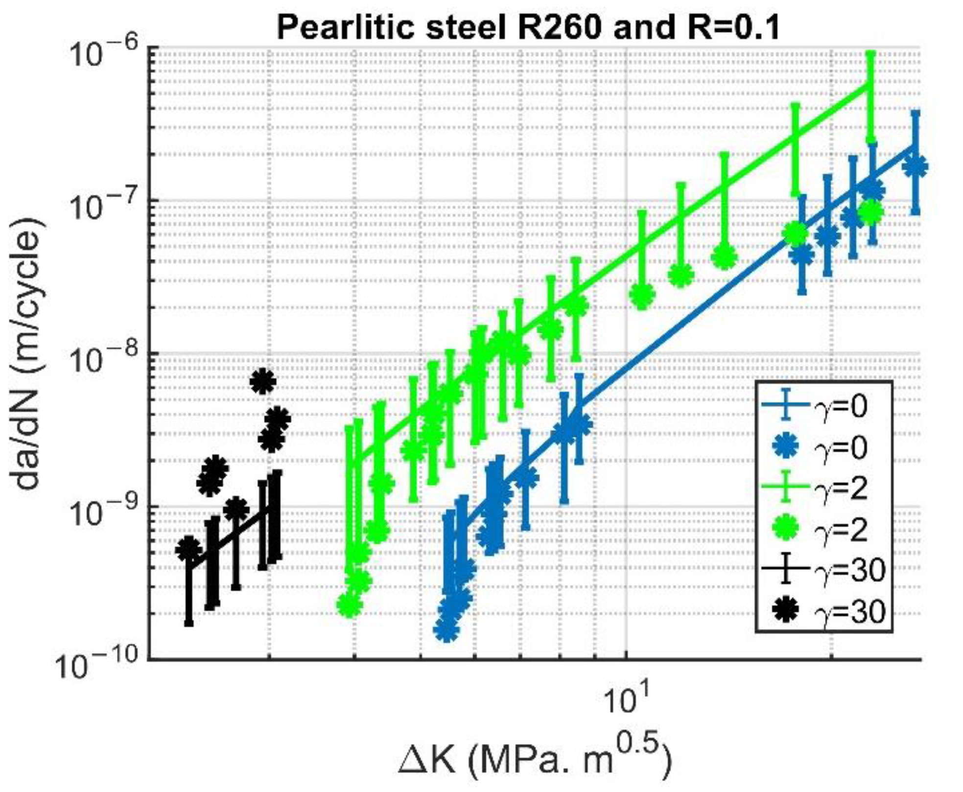
Figure 13.
Crack path for meshes representing the state of the R260 microstructure; (a). Undeformed; (b). Moderately deformed; (c). SPD; (d). Moderately deformed in T-A orientation; (e). SPD in T-A orientation.
Figure 13.
Crack path for meshes representing the state of the R260 microstructure; (a). Undeformed; (b). Moderately deformed; (c). SPD; (d). Moderately deformed in T-A orientation; (e). SPD in T-A orientation.
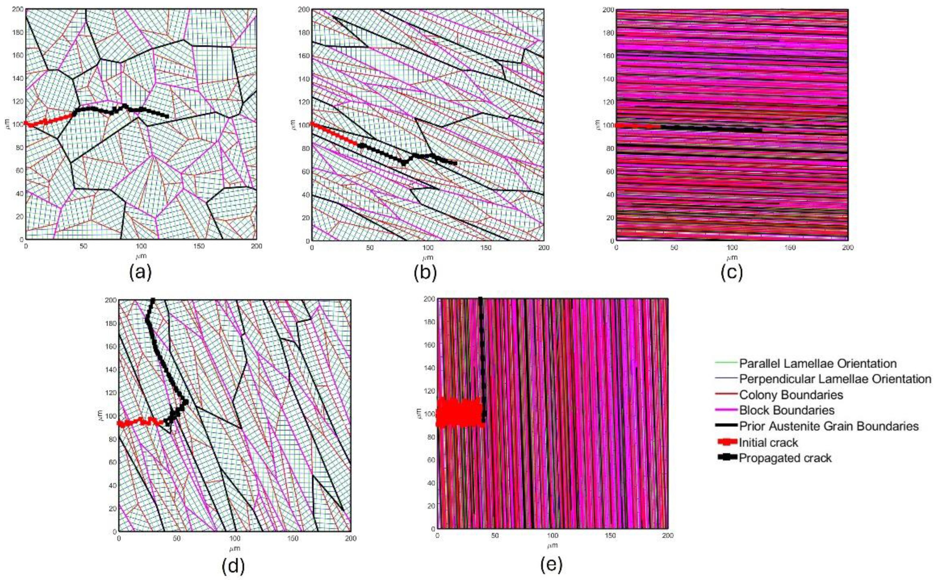
Figure 14.
Crack tortuosity values comparison for undeformed, moderately deformed, severely deformed, and moderately deformed in T-A orientation.
Figure 14.
Crack tortuosity values comparison for undeformed, moderately deformed, severely deformed, and moderately deformed in T-A orientation.
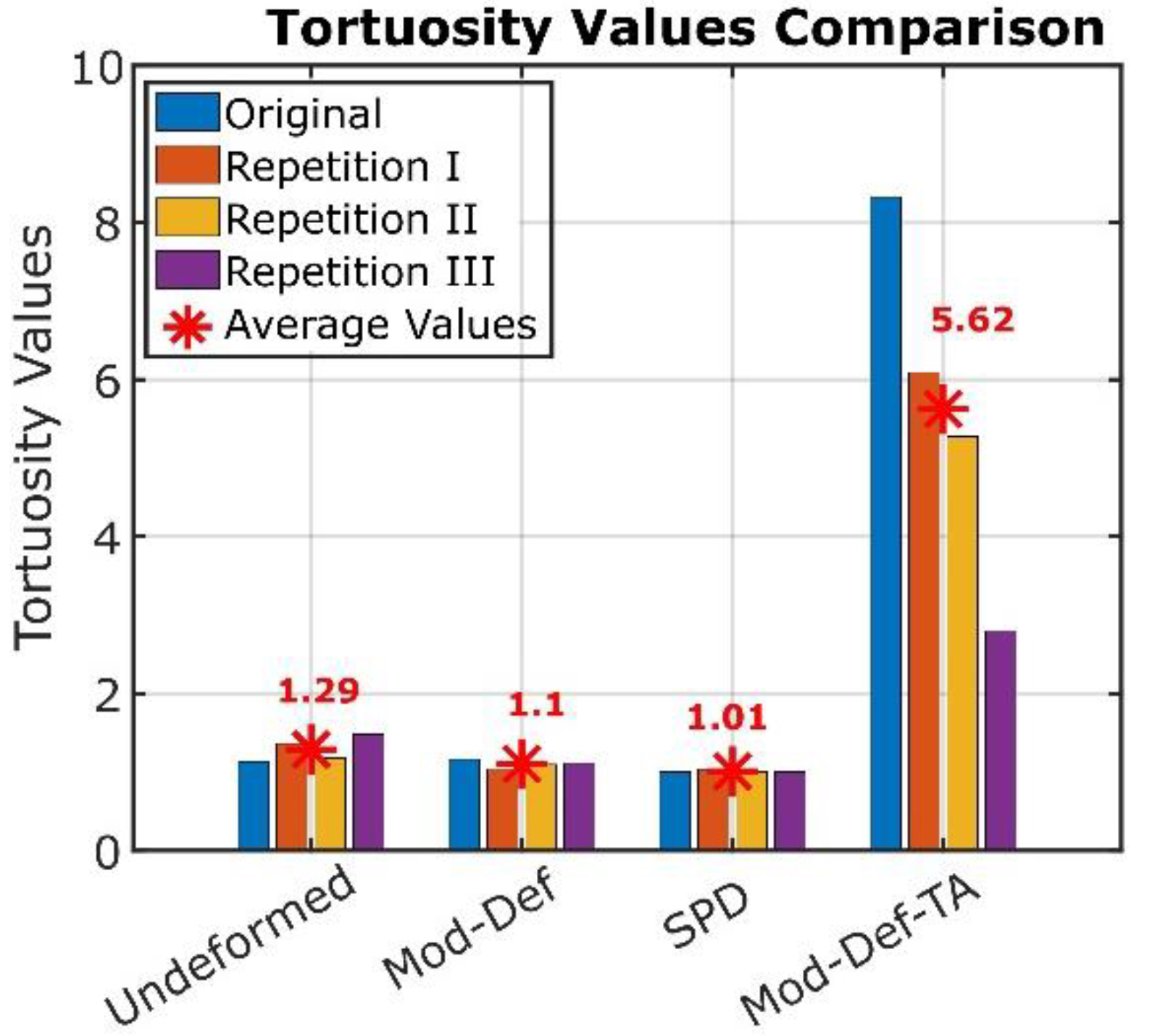
Figure 15.
(a). Comparison of the qualitative FCG rate between moderately and severely deformed mesh with adjusted values of and . (b). Qualitative FCG rate comparison between undeformed, moderately deformed and severely deformed meshes using and for undeformed, moderately deformed and severely deformed meshes.
Disclaimer/Publisher’s Note: The statements, opinions and data contained in all publications are solely those of the individual author(s) and contributor(s) and not of MDPI and/or the editor(s). MDPI and/or the editor(s) disclaim responsibility for any injury to people or property resulting from any ideas, methods, instructions or products referred to in the content. |
© 2025 by the authors. Licensee MDPI, Basel, Switzerland. This article is an open access article distributed under the terms and conditions of the Creative Commons Attribution (CC BY) license (http://creativecommons.org/licenses/by/4.0/).
Copyright: This open access article is published under a Creative Commons CC BY 4.0 license, which permit the free download, distribution, and reuse, provided that the author and preprint are cited in any reuse.


