
Submitted:
11 March 2025
Posted:
12 March 2025
You are already at the latest version
Abstract
The magnetic flux leakage (MFL) method is widely acknowledged as a highly effective non-destructive evaluation (NDE) technique for detecting local damage in ferromagnetic structures such as steel wire ropes. In this study, a multi-channel MFL sensor module was developed, incorporating a purpose-designed Hall sensor array and magnetic yokes specifically shaped for steel cables. To validate the proposed damage detection method, artificial damages of varying degrees were inflicted on wire rope specimens through experimental testing. The MFL sensor module facilitated the scanning of the damaged specimens and measurement of the corresponding MFL signals. In order to improve the signal-to-noise ratio, a comprehensive set of signal processing steps, including channel equalization and normalization, was implemented. Subsequently, the detected MFL distribution surrounding wire rope defects was transformed into MFL images. These images were then analyzed and processed utilizing an object detection method, specifically employing the YOLOv10 network, which enables accurate identification and localization of defects. Furthermore, a quantitative defect detection method based on image size was introduced, which is effective for quantifying defects using the dimensions of the anchor frame. The experimental results demonstrated the effectiveness of the proposed approach in detecting and quantifying defects in steel cables, which combines deep learning-based analysis of MFL images with the non-destructive inspection of steel cables.
Keywords:
Nondestructive inspection
; steel cable
; magnetic flux leakage
; YOLO
1. Introduction
Wire ropes are integral components extensively utilized in a diverse range of industries, and play crucial roles in critical applications such as lifting, towing, and suspension systems. The assurance of wire rope integrity and reliability assumes great significance in order to reduce the risks of accidents and equipment failures. However, the detection and assessment of defects within wire ropes present challenges due to their complex structure. Consequently, the development of effective non-destructive testing (NDT) methods has emerged as a pressing need to address these challenges and ensure the sustained performance and safety of wire ropes [1]. Wire rope defects can generally be categorized into two types: local defects (LF) and metal cross-section loss (LMA) [2]. In wire rope inspection, several mainstream NDT methods are available to detect and assess these defects. Visual inspection involves a thorough visual examination of the wire rope to identify visible defects. It relies on human inspectors to visually inspect the rope for surface irregularities. Ultrasonic testing (UT) [3] is another widely used method for wire rope inspection , which utilizes high-frequency sound waves to detect and evaluate defects in materials. By analyzing analyzing the reflected waves, UT can identify flaws such as cracks, corrosion, and internal discontinuities. Radiographic testing (RT) [4] employs X-rays or gamma rays to penetrate the wire rope and create an image that reveals internal defects, which is effective in detecting defects such as internal corrosion and voids within the rope structure. Eddy current testing (ECT) [5] utilizes electromagnetic induction to detect surface and subsurface defects in conductive materials. By measuring changes in electrical conductivity, ECT can identify defects such as cracks, corrosion, or variations in material properties. In addition, other testing methods for wire rope inspection include infrared thermography (IT) method [6,7], acoustic emission (AE) method [8] and metal magnetic memory (MMM) method [9]. In comparison to the aforementioned methods, magnetic flux leakage (MFL) [10,11] testing offers several advantages, including reliable effectiveness, robustness, convenience and rapid detection capabilities, thereby making it a more suitable and widely employed technique for wire rope inspection [12,13]. This method involves the application of a high-intensity magnetic field to magnetize the ferromagnetic material. In the presence of a discontinuous volume in the measured specimen, such as a defect, the magnetic induction lines leak out from the material in a saturation magnetization state. MFL testing enables the detection of these leaked magnetic flux lines using magnetic sensors, which facilitates the identification and assessment of wire rope defects.
With the continuous advancement of information processing technology, MFL defect detection techniques are gradually shifting towards automation and quantification. In this context, two-dimensional MFL signals often offer advantages over one-dimensional MFL signals in defect assessment. Based on two-dimensional MFL images, scholars have proposed two categories of defect assessment methods: model-based and model-free approaches. The model-based approach utilizes physical mechanisms to estimate the MFL signals surrounding the defects and recovers the dimensional information of defects through various optimization methods. Li et al. [14] introduced the Modified Harmony Search (MHS) algorithm based on a multiple selection opposition-based learning strategy to reconstruct defect dimensions. Peng et al. [15] utilized the combination-invariance property of MFL signals and performed combined operations on the measured MFL signals using a priori MFL signal set to approximate the defect contour. Long et al. [16] combined the characteristic approximation approach (CAA) with the magnetic dipole model-derived MFL signal distribution characteristics to achieve defect contour detection and improve defect recognition accuracy. The model-based approach yields accurate results but relies heavily on optimization algorithms, which is sensitive to parameter selection. In practical engineering applications, the complex parameters significantly increase the modeling difficulty and computational complexity. On the other hand, the model-free approach provide a faster solution for defect assessment. These methods construct a mapping model between signal sequence features and defect dimensions, without relying on a physical model. Artificial intelligence techniques are primarily employed in such approaches. Tan and Zhang [17] proposed a multi-frame image resolution enhancement method based on a giant magneto-resistance (GMR) sensor array, and achieved a quantitative identification rate of 91.43% for steel wire rope defects through the implementation of a radial basis function neural network. Lu et al. [18] introduced a defect dimension estimation method based on MFL imaging and visual transformation CNN (VT-CNN) theory, incorporating a visual transformation layer to accurately differentiate defects of different sizes. Yang et al. [19] presented a multi-MFL image detection algorithm based on the SSD network, achieving precise detection of defects at multiple scales. Yu et al. [20] improved the generalization ability of defect assessment model by constructing multi-domain features using the dynamic multi-domain feature input iterative stacking estimation network (WT STACK) for triaxial MFL signals. Wu et al. [21] proposed a defect reconstruction method that combines reinforcement learning with the classic iteration-based approach, improving the accuracy of defect reconstruction. Tu et al. [22] utilized the Dempster-Shafer evidence theory and Apriori algorithm for feature fusion in MFL signal processing, and employed a Stacking strategy to integrate LR, KNN and RF models, resulting in improved data adaptability and defect recognition rate for MFL defect identification.
The utilization of advanced algorithms in MFL image processing enhances the accuracy of defect detection, thereby facilitating the implementation of automated systems. However, these methods often suffer from slow detection speeds and lack visual intuitiveness during the detection process, which can impede their practical applicability in real-world applications. Consequently, ongoing research endeavors are directed towards enhancing the accuracy, efficiency and automation of these methods. In this study, a novel approach for wire defect detection is proposed, which employs a multi-channel MFL sensor module and integrates the YOLOv10 network. The MFL sensor module enables MFL imaging, while a filtering algorithm based on cable strand distribution features is proposed to enhance image quality. Subsequently, the YOLOv10 network is utilized for defect recognition. This integrated approach enhances the accuracy and efficiency of wire defect detection while also providing improved automation. As a result, faster and more intuitive detection results can be achieved. These advancements contribute to the development of more reliable and efficient wire rope inspection systems.
2. Methodology
2.1. Principle of Magnetic Flux Leakage
The fundamental principle of wire rope defect detection using the MFL method in nondestructive testing was illustrated in Figure 1. In this method, the steel wire rope is enclosed by two sets of permanent magnet arrays, each consisting of eight neodymium magnets. These permanent magnet arrays are specially positioned along with the magnetic yoke to create a magnetic circuit surrounding the wire rope. These components form a magnetic circuit that passes through the wire rope, in which case the wire rope is magnetized into a saturated state. Under normal conditions, the magnetic flux within the wire rope remains constant, indicating the absence of any magnetic leakage signals. However, when defects are present within the wire rope, such as corrosion, wire breakage or other forms of damage, the magnetic permeability at the defect location decreases. This decrease in permeability leads to an increase in magnetic reluctance, which subsequently causes the magnetic induction lines to deviate from their regular path. Consequently, there is a diffusion of magnetic flux towards the surface of the defect, which results in the generation of a magnetic leakage field. This magnetic leakage field directly indicates changes in the magnetic flux caused by defects within the wire rope. By measuring and analyzing this magnetic leakage field, it becomes possible to identify the location and extent of the defects present in the wire rope. To quantitatively assess the extent of damage in the wire rope, the leakage magnetic field data is obtained through magnetic-sensitive elements, which captures variations in the magnetic field surrounding the defects present in the wire rope. The collected data is subsequently subjected to analysis and processing techniques to extract relevant information necessary for the identification and characterization of the defects.
To describe the distribution of the three-dimensional MFL, Dutta et al. [23] developed a magnetic dipole model and derived the analytical expression of the magnetic field in the air dielectric space above the defect. In this study, a simplified analytical dipole model is developed for a cylindrical surface defect on a wire rope, as depicted in Figure 2. Notably, owing to the orientation of the wire rope, the MFL field components of this particular defect can be categorized into three distinct types: the Tangential component (), the Axial component (), and the Radial component (). The specific dipole model of the defect is shown in a Cartesian Coordinate System in Figure 3, where the defect depth is denoted as and the radius as . In this coordinate system, , and represent the unit vectors along the -axis, -axis and -axis, respectively.
Therefore, the surface magnetic charge of the element S can be expressed as [23]:
where denotes the surface magnetic charge density and denotes the magnetization vector.
Therefore, at any point located above the defect, the magnetic field from the element S can be expressed as:
where represents the vector from the defect element to the point .
By integrating the magnetic field contributions from all the elements on the defect surface S, the complete MFL distribution at point can be expressed as:
Then the position vector can be expressed as:
Thus, the whole leakage magnetic field intensity can be converted into:
In accordance with Eq. 5, the distribution of the leakage magnetic field is simulated through constructing defects. Specifically, to facilitate the imaging of magnetic leakage near the cable surface, our experimental focus primarily lies in the detection of the radial magnetic field component within the cable cross-section. Figure 4 presents a visualization of the typical normalized spatial distribution of this radial component of the leakage magnetic field intensity. Along the y-axis scanning direction, it’s noticeable that exhibits a discernible pattern. It initially undergoes an increase, followed by a subsequent decrease, culminating in peak absolute values at the edges on either side of the defect. Notably, this intensity distribution is symmetrically centered around the central position of the defect. This characteristic enables us to derive valuable spatial information regarding the defects based on the distribution of .
2.2. Principle of YOLOv10 Network
Deep learning-based object detection methods can be generally classified into two types: one-stage detectors and two-stage detectors. The two-stage detectors, represented by notable architectures such as Faster R-CNN [24], Mask R-CNN [25] and Cascade R-CNN [26], generate regional proposal and perform object classification sequentially. As a popular two-stage detector, Fast R-CNN exhibited inefficiencies in learning and execution speed due to its separate candidate area generation module, decoupled from the CNN backbone. On the other hand, one-stage detectors, which involves approaches like YOLO [27], SSD [28], SqueezeDet [29], FCOS[30] and Efficientdet [31], handle both regional proposal and classification tasks simultaneously, effectively addressing both localization and classification tasks in a unified framework.
The initial YOLO proposed by Redmon et al. [27] presented a unified approach, which requires precise manual annotation for bounding boxes and integrates all object detection components within a single neural network. By leveraging global image features, YOLO predicts bounding boxes and class probabilities for all objects in a single forward pass, making it notably faster than traditional two-stage detectors. It formulates the detection process as a regression problem. The input image is divided into an S×S grid, with each grid cell predicting B bounding boxes along with their respective confidences and class probabilities. The network parameters are iteratively adjusted through backpropagation during training to minimize the detection loss, which includes localization loss, confidence loss, and class prediction loss. The utilization of a unified network enables YOLO to achieve impressive real-time performance while maintaining competitive detection accuracy.
With successive versions of YOLO algorithm, a pattern of enhanced accuracy coupled with sustained high-speed processing has emerged. YOLOv10, similar to its predecessor YOLOv8, retains the fundamental architectural divisions; however, it introduces a series of optimizations that further elevate algorithmic performance, which is lighter and faster. This innovative iteration’s architectural layout is graphically represented in Figure 5. The YOLOv10 series encompasses five model versions: YOLOv10N, YOLOv10S, YOLOv10M, YOLOv10L, and YOLOv10X. While these models share a core structural foundation, differences lie in the scaling of modules and convolutional kernels. This scaling influences the models’ complexity and dimensions, with YOLOv10N being the smallest and YOLOv10X being the largest. The focus of the current experiment is conducted based on the YOLOv10N variant.
In terms of data augmentation, YOLOv10 employs mosaic data augmentation, which involves composing images from smaller patches. This technique amplifies the model’s adeptness at detecting objects across varying scales. The architecture of YOLOv10 comprises three essential segments: the backbone network, the neck network, and the head network. The backbone segment functions as the core feature extractor and comprises the Conv module, C2f module, C2fCIB module, SPPF module, and PSA module. The Conv module includes standard convolutional operations, batch normalization, and the SiLU activation function. The C2f module is inspired by the Bottleneck design philosophy, which partitions the feature map along a specific dimension. This partitioning enhances the model’s nonlinear representation capacity, thereby improving its proficiency in processing complex image features. It integrates two 1×1 convolutions, a sequence of bottleneck layers, and a final 1×1 convolution for concatenation. The SPPF module enhances the network’s receptive field and addresses multi-scale challenges. The C2fCIB module introduces a Compact Inverted Block (CIB) structure, which provides higher efficiency and accuracy compared to previous versions. To address computational complexity and memory footprint, YOLOv10 presents an efficient Partial Self-Attention (PSA) module design, as shown in Figure 5. Specifically, it comprises a Multi-Head Self-Attention (MHSA) module and a Feed-Forward Network (FPN). The neck component of YOLOv10 employs PANet [32] and FPN [33] operations. PANet contributes to precise high-level feature localization, while FPN leverages upsampling for potent low-level semantic features. This dynamic combination enhances object detection capabilities. The head network employs an NMS-free training strategy for YOLOS, incorporating dual label assignments and a consistent matching metric, thereby achieving enhanced efficiency and competitive performance. These advancements significantly improve overall performance and efficiency, with a notable enhancement in small object detection, rendering the approach particularly well-suited for MFL image defect detection tasks.
3. Experimental Setup
3.1. Establishment of Inspection System
The steel wire rope inspection system is a meticulously engineered apparatus, consisting of four fundamental components: a magnetizer, a Hall sensor array, a data acquisition system, and an equidistant encoder. A schematic view and a photographic view of this system are presented in Figure 6 and Figure 7, respectively, providing both a conceptual representation and a visual depiction of its structural design and functionality.
The magnetizer serves as the linchpin of the system, comprised of permanent magnet arrays designed to magnetize the steel wire rope to a state of saturation, thereby enabling optimal sensitivity to the MFL detection technique. In the experiment, each neodymium magnet exhibits a residual magnetic field strength of approximately 1.4 Tesla. The Hall sensor array, as present in Figure 8, which transforms magnetic signals into electrical ones, capturing the normal component of the leakage magnetic field for yielding comprehensive data. The equidistant encoder is affixed to one of the collection system’s guide wheels, where it encodes the linear distance covered by the wire rope during the inspection process, operating at a sampling frequency of 1000 Hz. It operates in synchronization with the system, triggering the simultaneous sampling of multi-channel magnetic flux leakage signals when encoder signals are activated. This data acquisition mechanism ensures the maintenance of precise spatial accuracy throughout the inspection. In the experiment, the steel wire rope is guided through the guide wheel and passes through the channel wall, as depicted in Figure 8. The control system functions as the central command unit within the inspection setup, which is responsible for sending control instructions to the detection system and receiving feedback data in return. This pivotal role in commanding the system and managing the bidirectional flow of information ensures the smooth orchestration of the inspection process, enabling real-time control and data acquisition.
Expanding on the fundamental components outlined above, the comprehensive detection process of the entire system is elaborated in Figure 9, with a specific focus on the identification of the leakage magnetic field. It issues instructions to the controller to commence data collection, and this process begins when the equidistant encoder outputs a signal. Once a set of data is collected, the controller transmits the received signals back to the server and handheld devices through either serial communication or WiFi, facilitating real-time display of the magnetic flux leakage signals relevant to the detected defects. The collaborative synergy of these components serves as a cornerstone, guaranteeing the efficacy and precision of the system in the domain of non-destructive steel wire rope evaluation.
3.2. Establishment of Dataset
In the experimental setup, the steel wire rope, as depicted in Figure 10, comprises six external strands, each having a diameter of 38mm, which are arranged in a right-hand direction. Building upon this specimen, various steel wire rope specimens with different defect sizes were prepared. These defects are categorized into two primary types: LF (Local Flaw) and LMA (Loss of Metallic Cross-Sectional Area). A typical LF defect is illustrated in Figure 10, while a typical LMA defect is shown in Figure 10. It is noteworthy that LMA defects exhibit a larger loss of cross-sectional area around the circumferential direction of the cable compared to LF defects. Recognizing on the distinction between LF and LMA, the experiment further enhances defect assessment by introducing an evaluation of defect severity based on the extent of damage along the cable’s axial direction. This classification, which considers different LF and LMA defects based on their length along the cable’s axis, allows for a more detailed and precise defect assessment.
The MFL signals collected from the 32-Hall sensor array, corresponding to various defect categories, are subjected to detailed analysis. These signals undergo transformation, wherein they are laid out in a horizontal plane, as visually represented in Figure 11. This processing step allows for the conversion of the MFL signals into a comprehensive MFL image, enabling precise defect localization in both circumferential and axial directions. This approach substantially improves the clarity and precision of defect localization, which provides a more intuitive and accurate resolution.
Figure 11 provides a three-dimensional visual representation of the raw MFL image without defect, which is derived from the signals captured by the Hall sensor array. It is worth noting that the MFL signals exhibit a certain degree of periodicity along the axial direction of the wire rope, which allows us to perform baseline correction using a sliding window averaging method in that direction. However, in the circumferential direction, voltage discrepancies among channels can obscure the identification of defects, posing a significant challenge. To address this, a method based on channel-wise data normalization is introduced. Initially, the peak-to-peak detection method is used to identify all peak and valley values in each channel. Subsequently, the average of all peak values and the average of all valley values are calculated for each channel. The difference between these two values represents the average peak-to-valley value for that specific channel. Finally, one channel’s peak-to-valley value is selected as a reference, and the other channels are compensated in comparison to this reference. Following the normalization of peak-to-valley values, a three-dimensional visual representation of the MFL image displays reduced differences between channels, as shown in Figure 11.
To alleviate the computational complexity of the neural network, the dataset utilizes two-dimensional MFL gray-scale images captured from the top view of the x-y plane. Figure 12 and Figure 12 respectively showcase typical MFL images, one devoid of defects and the other encompassing both LMA and LF defects. Notably, these images exhibit a distinctive periodic pattern within the signal traces. This pattern, stemming from the inherent structural characteristics of the wire rope, can influence defect assessment to some extent. Therefore, a filtering algorithm is incorporated based on the cable strand inclination angle, to ameliorate the influence of strand-related textural features. This process yields an MFL image without the special textures, exemplified in Figure 12 and Figure 12, wherein the positions of defects and their corresponding dimensions are prominently visible. Here, the yellow boxes indicate LF defects, while the red boxes highlight LMA defects.
A magnetic leakage image dataset was constructed by collecting data of sample ropes within the laboratory setting. This dataset encompasses a total of 256 samples, with each sample featuring different types of defects, including 1,678 instances of LF defects and 981 cases of LMA defects. Subsequent to the compilation of this labeled dataset, an allocation strategy was employed, partitioning the dataset into three subsets: 80% was designated as the training set, 10% for validation, and the remaining 10% for testing purposes. The training subset will be utilized as the input for training the YOLOv10 network model, enabling its development and evaluation.
4. Experiment and Results
4.1. Dataset
Based on the methodology described in Section 3.2, the dataset was established by collecting data from sample ropes in a laboratory setting. This dataset consists of 256 samples, encompassing 1,678 instances of LF defects and 981 instances of LMA defects. Following the compilation of this labeled dataset, an allocation strategy was implemented, dividing the dataset into three subsets: 80% for training, 10% for validation, and 10% for testing. The training subset is utilized to train the YOLOv10 network model, thereby facilitating its development and evaluation.
4.2. Parameters Setting
In the YOLOv10 training phase, the Stochastic Gradient Descent with Momentum (SGDM) optimization algorithm is applied, utilizing specific hyperparameters detailed in Table 1.
Throughout training, input images undergo augmentation and resizing before being fed into the CNNs. Following this, predictions of bounding box information are generated based on anchor boxes. Subsequently, the loss function is employed to calculate the disparity between the predicted bounding boxes and the ground truth bounding boxes. During the testing phase, well-trained neural networks process input images with high efficiency, particularly benefiting from the one-to-one branch structure.
4.3. Evaluation Indicator
The commonly used evaluation metrics for object detection include precision (P), recall (R), and mean Average Precision (). Precision denotes the probability that all positive samples detected by the model are actual positive samples, while recall represents the probability that the model detects positive samples within the actual positive samples. Precision and recall are respectively defined by Equation 6 and Equation 7:
Here, is the number of correctly detected defective samples, is the number of non-defective samples falsely identified as defective, is the number of defective samples incorrectly recognized. Furthermore, is a comprehensive metric considering both precision (P) and recall (R). A higher value indicates a higher detection accuracy of the model. It is defined as:
4.4. Results
The typical prediction results are illustrated in Figure 13, showcasing the network’s ability to provide distinct predictive analyses for different defects, including LMA and LF. Additionally, the The confusion matrix depicting the two defect classes is visualized in Figure 13. The detection precision for LF defects is 81%, while the detection precision for LMA defects is 69%. Specifically, the detection accuracy for LF is notably high, whereas the detection accuracy for LMA defects is comparatively lower. This discrepancy can be attributed to the complex nature of the texture features of LMA defects, which span across multiple cables, making the semantic information relatively intricate and prone to confusion compared to LF defects.
5. Conclusion and Discussion
In summary, this study has demonstrated the efficacy of preprocessing multi-channel one-dimensional magnetic leakage signals and their transformation into magnetic leakage images. This approach greatly facilitates two-dimensional defect localization and enhances the resolution and analysis of defect detection. Leveraging advanced deep learning algorithms, a effective real-time defect detection based on magnetic flux leakage technology has been achieved, thereby improving the efficiency and accuracy of the detection process. The utilization of the enhanced YOLOv10 network has enabled the analysis and processing of magnetic leakage images, yielding precise information regarding the positions and sizes of detected defects. This methodology significantly enhances the effectiveness of magnetic leakage detection in wire ropes. Furthermore, the expansion of the sample dataset has proven instrumental in continuously enhancing the accuracy of non-destructive testing for steel wire ropes using magnetic leakage images. It has enabled the synchronous classification detection of traditional wire rope defect types, encompassing both local defects and section loss. The fusion of deep learning networks with magnetic leakage images has paved the way for the integration of cutting-edge computer vision algorithms into the domain of electromagnetic nondestructive testing, ultimately contributing to the advancement and efficacy of electromagnetic nondestructive testing techniques.
Author Contributions
Conceptualization, M.Z.,Z.F. and D.N.; methodology, Z.F.,B.J.and M.Z.; software, M.Z., J.Z. and Z.F.; validation, M.Z. and Z.F.; formal analysis, M.Z.,B.J. and F.D.; investigation, M.Z., Z.F.and J.Z.; resources, M.Z. and B.J.; data curation, M.Z., F.D. and Z.F.; writing—original draft preparation, M.Z.,Z.F. and J.Z.; writing—review and editing, M.Z.,F.D.,and N.D.; supervision, M.Z. and N.D.; project administration, M.Z.,B.J. and N.D. All authors have read and agreed to the published version of the manuscript.
Funding
This research was supported by the Guangdong Province Key Construction Discipline Research Ability Enhancement Project (Grant Number: 2024ZDJS071).
Institutional Review Board Statement
Not applicable.
Informed Consent Statement
Not applicable.
Data Availability Statement
The data presented in this study are available on request from the corresponding author.
Acknowledgments
The author would like to thank Mr. Song Lu, Mr Zongguo Yang and Mr. Zhao Zhang for his kindly suggestions in the scenario requirements definition and experiments method.
Conflicts of Interest
The authors declare no conflict of interest.
References
- Zhou, P.; Zhou, G.; Zhu, Z.; He, Z.; Ding, X.; Tang, C. A Review of Non-Destructive Damage Detection Methods for Steel Wire Ropes. Applied Sciences 2019, 9. [Google Scholar] [CrossRef]
- Liu, S.; Sun, Y.; Jiang, X.; Kang, Y. A review of wire rope detection methods, sensors and signal processing techniques. Journal of Nondestructive Evaluation 2020, 39, 1–18. [Google Scholar]
- Rostami, J.; Tse, P.W.; Yuan, M. Detection of broken wires in elevator wire ropes with ultrasonic guided waves and tone-burst wavelet. Structural Health Monitoring 2020, 19, 481–494. [Google Scholar]
- Chakhlov, S.; Anpilogov, P.; Batranin, A.; Osipov, S.; Zhumabekova, S.; Yadrenkin, I. Generation and analysis of wire rope digital radiographic images. In Proceedings of the IOP Conference Series: Materials Science and Engineering. IOP Publishing, Vol. 132; 2016; p. 012008. [Google Scholar]
- Feng, B.; Deng, K.; Wang, S.; Chen, S.; Kang, Y. Theoretical Analysis on the Distribution of Eddy Current in Motion-Induced Eddy Current Testing and High-Speed MFL Testing. Journal of Nondestructive Evaluation 2022, 41, 59. [Google Scholar] [CrossRef]
- Xia, H.; Yan, R.; Wu, J.; He, S.; Zhang, M.; Qiu, Q.; Zhu, J.; Wang, J. Visualization and quantification of broken wires in steel wire ropes based on induction thermography. IEEE Sensors Journal 2021, 21, 18497–18503. [Google Scholar] [CrossRef]
- Xu, L.; Hu, J. A method of defect depth recognition in active infrared thermography based on GRU networks. Applied Sciences 2021, 11, 6387. [Google Scholar]
- Xin, H.; Cheng, L.; Diender, R.; Veljkovic, M. Fracture acoustic emission signals identification of stay cables in bridge engineering application using deep transfer learning and wavelet analysis. Advances in Bridge Engineering 2020, 1, 1–16. [Google Scholar]
- Juraszek, J. Residual magnetic field for identification of damage in steel wire rope. Archives of Mining Sciences 2019, 64, 79–92. [Google Scholar] [CrossRef]
- Liu, S.; Sun, Y.; Jiang, X.; Kang, Y. A new MFL imaging and quantitative nondestructive evaluation method in wire rope defect detection. Mechanical Systems and Signal Processing 2022, 163, 108156. [Google Scholar] [CrossRef]
- Donglai Zhang, Min Zhao, Z.Z. Quantitative inspection of wire rope discontinuities using magnetic flux leakage imaging. Journal of Nondestructive Evaluation 2012, 70, 872–878. 2012; 70, 872–878.
- Peng, X.; Anyaoha, U.; Liu, Z.; Tsukada, K. Analysis of magnetic-flux leakage (MFL) data for pipeline corrosion assessment. IEEE Transactions on Magnetics 2020, 56, 1–15. [Google Scholar]
- Donglai Zhang, Min Zhao, Z.Z.S.P. Characterization of wire rope defects with gray level co-occurrence matrix of magnetic flux leakage images. Journal of Nondestructive Evaluation 2013, 32, 37–43.
- Li, F.; Feng, J.; Zhang, H.; Liu, J.; Lu, S.; Ma, D. Quick reconstruction of arbitrary pipeline defect profiles from MFL measurements employing modified harmony search algorithm. IEEE Transactions on Instrumentation and Measurement 2018, 67, 2200–2213. [Google Scholar]
- Peng, L.; Huang, S.; Wang, S.; Zhao, W. An element-combination method for arbitrary defect reconstruction from MFL signals. In Proceedings of the 2020 IEEE International Instrumentation and Measurement Technology Conference (I2MTC). IEEE; 2020; pp. 1–6. [Google Scholar]
- Long, Y.; Huang, S.; Peng, L.; Wang, S.; Zhao, W. A characteristic approximation approach to defect opening profile recognition in magnetic flux leakage detection. IEEE Transactions on Instrumentation and Measurement 2021, 70, 1–12. [Google Scholar]
- Tan, X.; Zhang, J. Evaluation of Composite Wire Ropes Using Unsaturated Magnetic Excitation and Reconstruction Image with Super-Resolution. Applied Sciences 2018, 8. [Google Scholar] [CrossRef]
- Lu, S.; Feng, J.; Zhang, H.; Liu, J.; Wu, Z. An estimation method of defect size from MFL image using visual transformation convolutional neural network. IEEE Transactions on Industrial Informatics 2018, 15, 213–224. [Google Scholar] [CrossRef]
- Yang, L.; Wang, Z.; Gao, S. Pipeline magnetic flux leakage image detection algorithm based on multiscale SSD network. IEEE Transactions on Industrial Informatics 2019, 16, 501–509. [Google Scholar]
- Yu, G.; Liu, J.; Zhang, H.; Liu, C. An iterative stacking method for pipeline defect inversion with complex MFL signals. IEEE Transactions on Instrumentation and Measurement 2019, 69, 3780–3788. [Google Scholar] [CrossRef]
- Wu, Z.; Deng, Y.; Liu, J.; Wang, L. A reinforcement learning-based reconstruction method for complex defect profiles in MFL inspection. IEEE Transactions on Instrumentation and Measurement 2021, 70, 1–10. [Google Scholar] [CrossRef]
- Tu, F.; Wei, M.; Liu, J. A coupling model of multi-feature fusion and multi-machine learning model integration for defect recognition. Journal of Magnetism and Magnetic Materials 2023, 568, 170395. [Google Scholar] [CrossRef]
- Dutta, S.M.; Ghorbel, F.H.; Stanley, R.K. Dipole modeling of magnetic flux leakage. IEEE Transactions on Magnetics 2009, 45, 1959–1965. [Google Scholar] [CrossRef]
- Ren, S.; He, K.; Girshick, R.; Sun, J. Faster r-cnn: Towards real-time object detection with region proposal networks. Advances in neural information processing systems 2015, 28. [Google Scholar]
- He, K.; Gkioxari, G.; Dollár, P.; Girshick, R. Mask r-cnn. In Proceedings of the Proceedings of the IEEE international conference on computer vision, 2017, pp.
- Cai, Z.; Vasconcelos, N. Cascade r-cnn: Delving into high quality object detection. In Proceedings of the Proceedings of the IEEE conference on computer vision and pattern recognition, 2018, pp.
- Redmon, J.; Divvala, S.; Girshick, R.; Farhadi, A. You only look once: Unified, real-time object detection. In Proceedings of the Proceedings of the IEEE conference on computer vision and pattern recognition, 2016, pp.
- Liu, W.; Anguelov, D.; Erhan, D.; Szegedy, C.; Reed, S.; Fu, C.Y.; Berg, A.C. Ssd: Single shot multibox detector. In Proceedings of the Computer Vision–ECCV 2016: 14th European Conference, Amsterdam, The Netherlands, 2016, Proceedings, Part I 14. Springer, 2016, October 11–14; pp. 21–37.
- Wu, B.; Iandola, F.; Jin, P.H.; Keutzer, K. Squeezedet: Unified, small, low power fully convolutional neural networks for real-time object detection for autonomous driving. In Proceedings of the Proceedings of the IEEE conference on computer vision and pattern recognition workshops, 2017, pp.
- Tian, Z.; Shen, C.; Chen, H.; He, T. Fcos: Fully convolutional one-stage object detection. In Proceedings of the Proceedings of the IEEE/CVF international conference on computer vision, 2019, pp.
- Tan, M.; Pang, R.; Le, Q.V. Efficientdet: Scalable and efficient object detection. In Proceedings of the Proceedings of the IEEE/CVF conference on computer vision and pattern recognition, 2020, pp.
- Liu, S.; Qi, L.; Qin, H.; Shi, J.; Jia, J. Path aggregation network for instance segmentation. In Proceedings of the Proceedings of the IEEE conference on computer vision and pattern recognition, 2018, pp.
- Lin, T.Y.; Dollár, P.; Girshick, R.; He, K.; Hariharan, B.; Belongie, S. Feature pyramid networks for object detection. In Proceedings of the Proceedings of the IEEE conference on computer vision and pattern recognition, 2017, pp.
Figure 1.
Schematic of excitation structure and detect sensor.
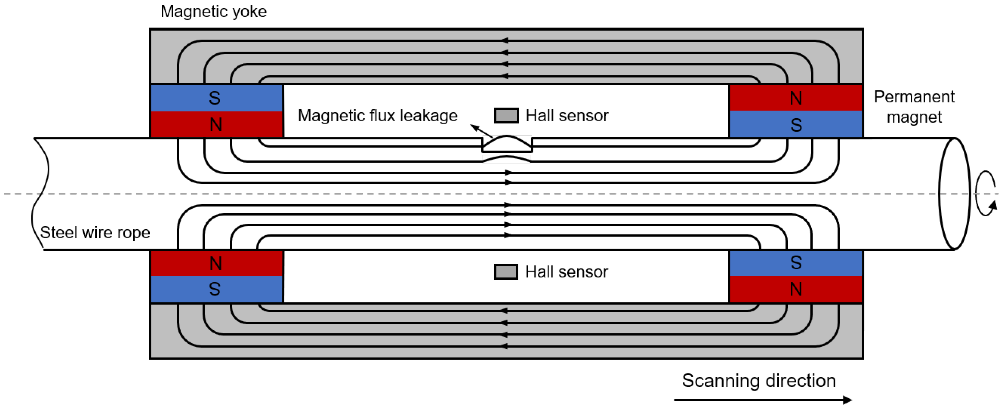
Figure 2.
Schematic of the dipole model on a wire rope.
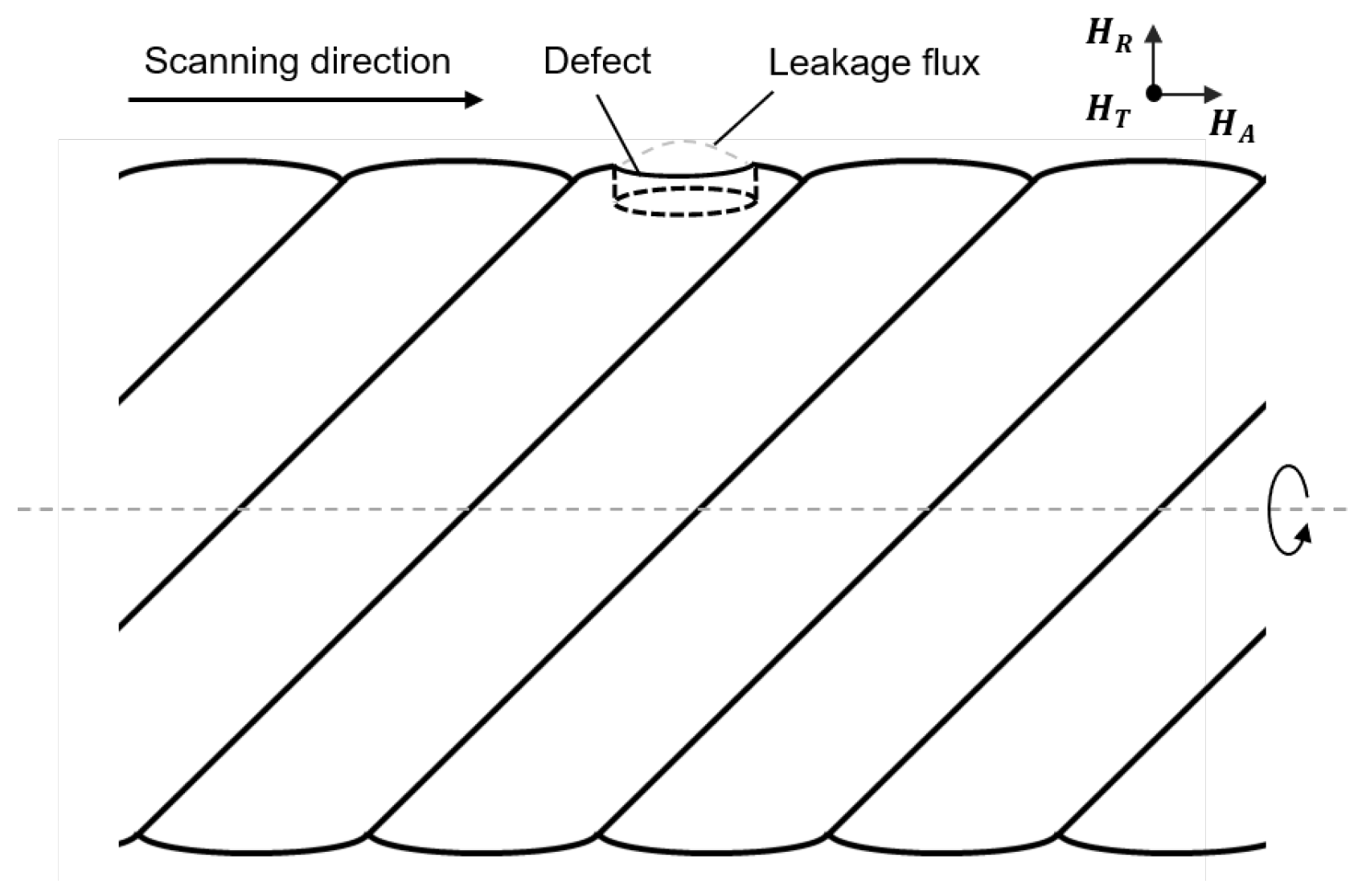
Figure 3.
Cylindrical defect magnet dipole model (a) 3-D view (b) Top view.
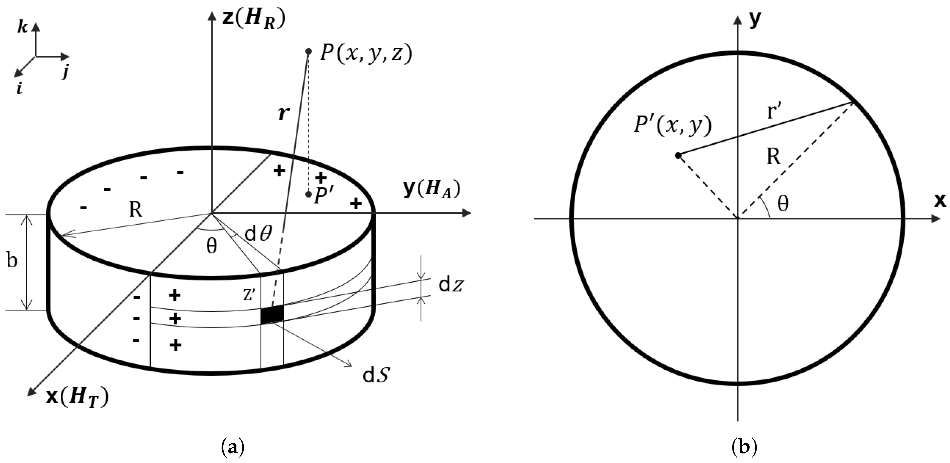
Figure 4.
Normalized radial component of leakage magnetic field spatial distribution (a) 3-D view (b) Top view.
Figure 4.
Normalized radial component of leakage magnetic field spatial distribution (a) 3-D view (b) Top view.
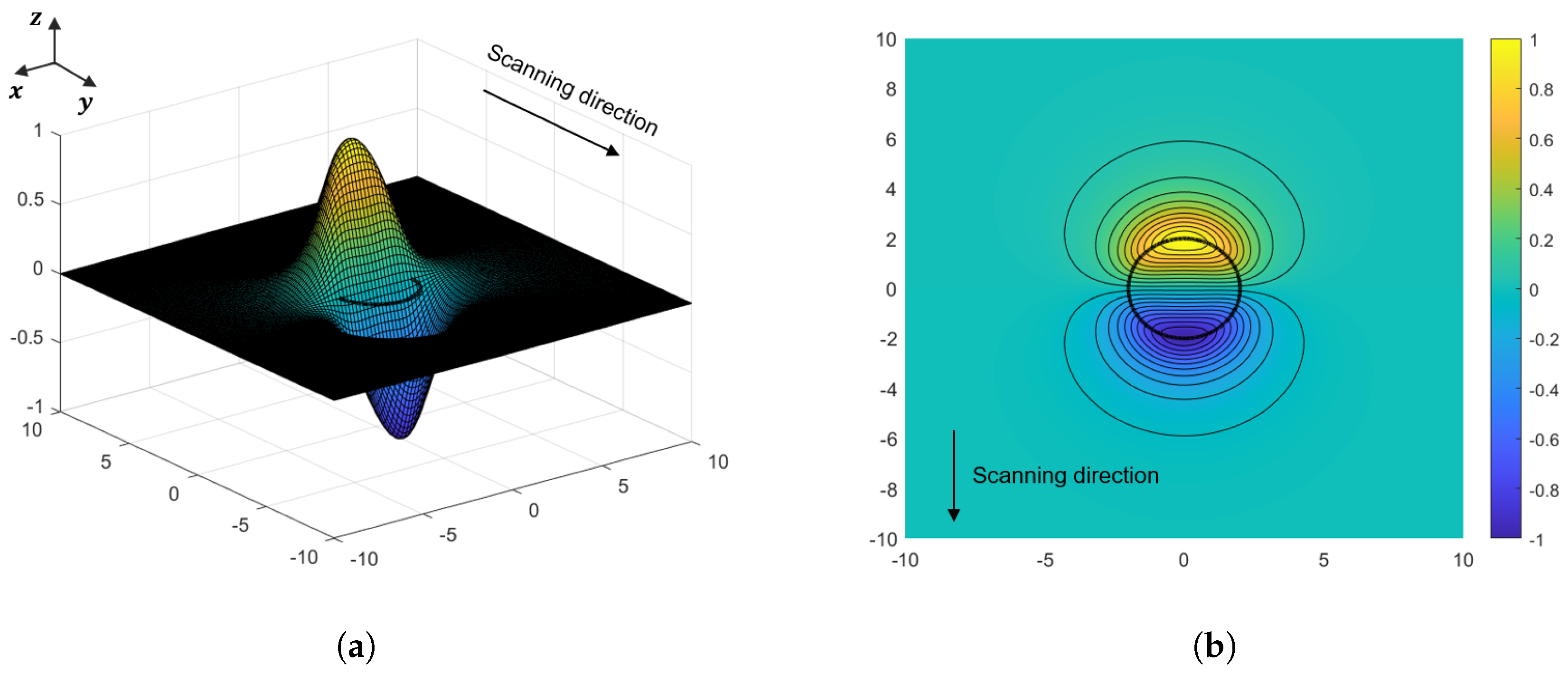
Figure 5.
Architecture of YOLOv10.
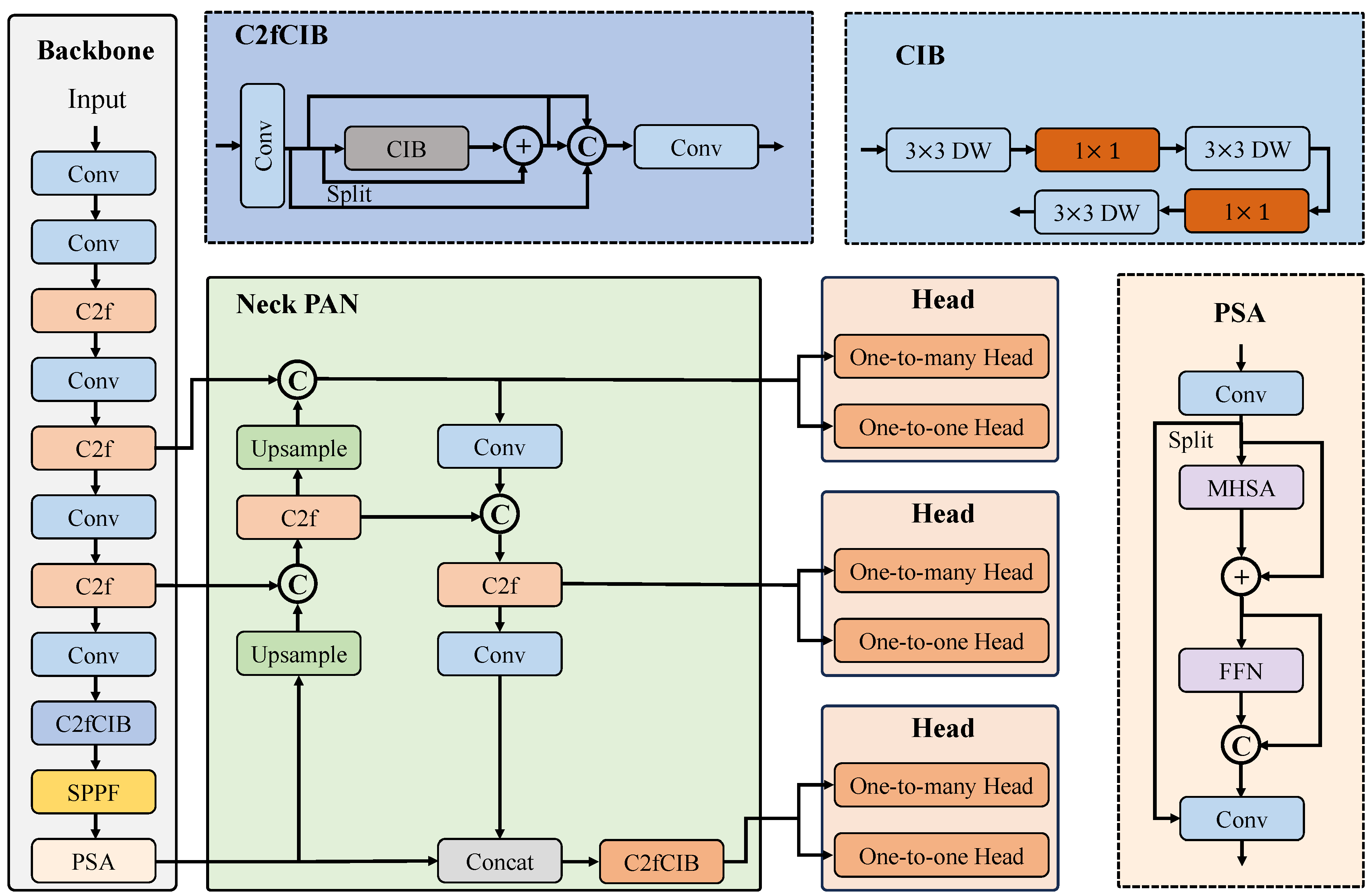
Figure 6.
Schematic view of system structure.
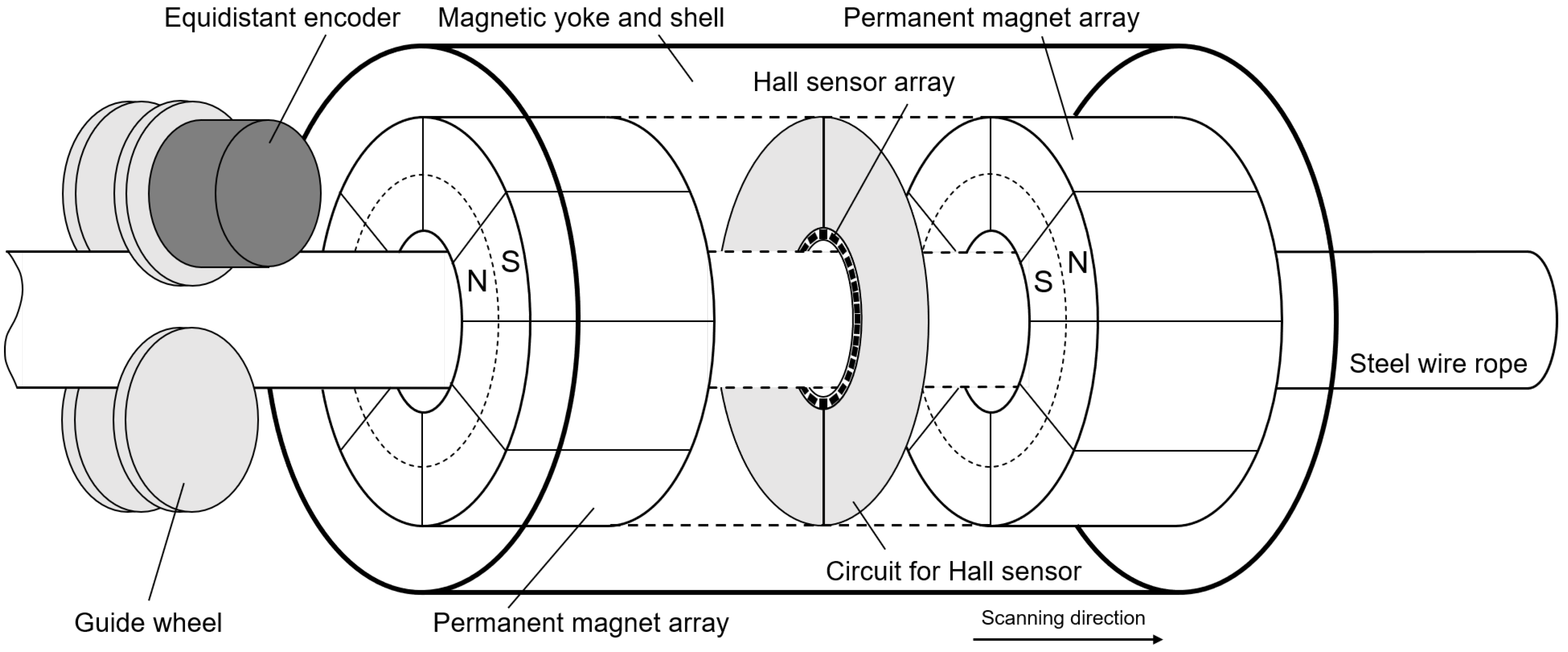
Figure 7.
Photographic view of system structure.
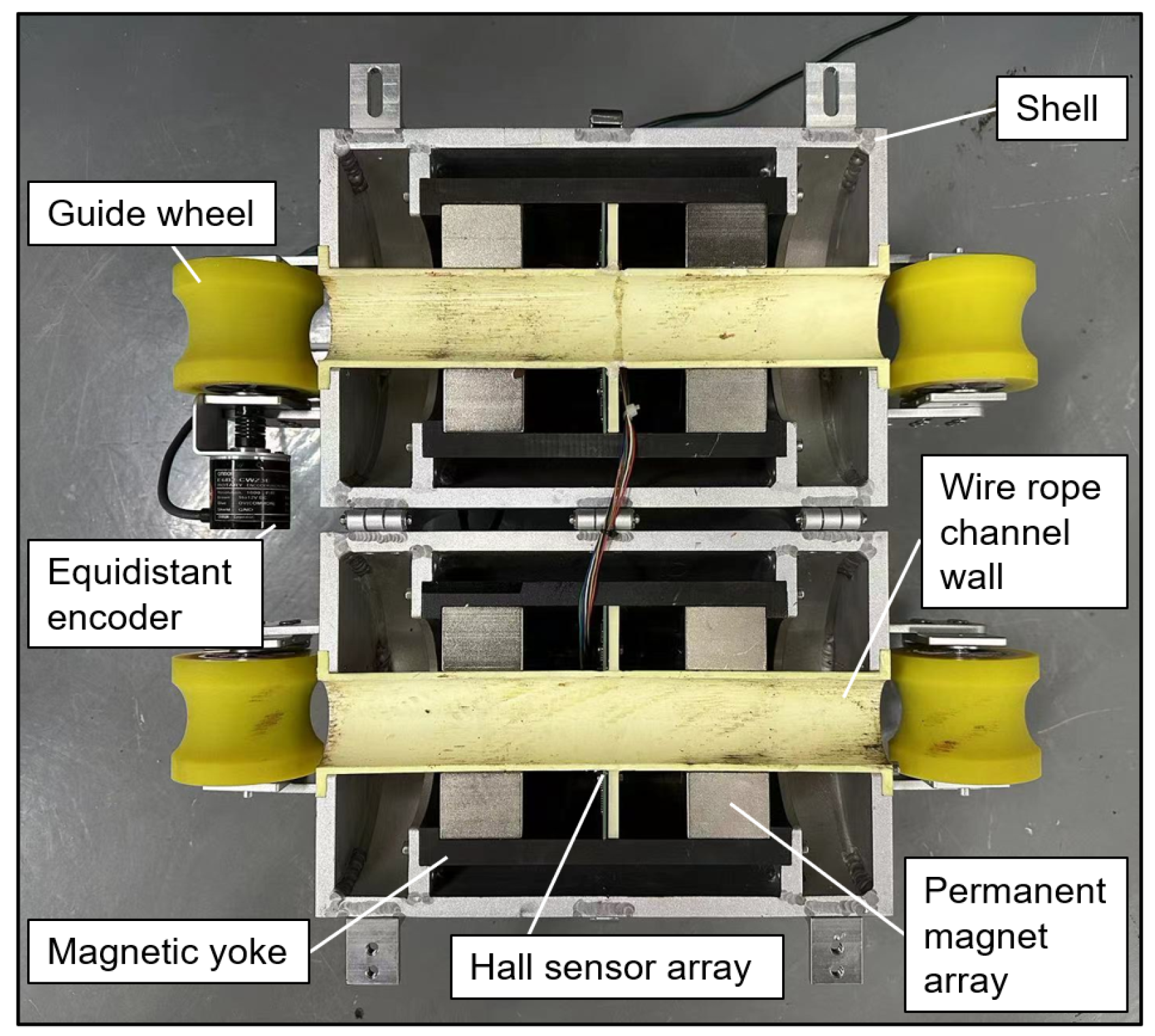
Figure 8.
Experimental diagram (a) Photographic view of Hall sensor array (b) Diagram of experimental assembly.
Figure 8.
Experimental diagram (a) Photographic view of Hall sensor array (b) Diagram of experimental assembly.
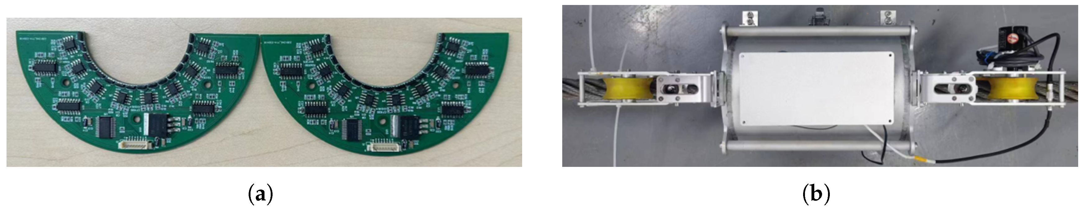
Figure 9.
Flaw diagram of leakage magnetic field acquisition system.
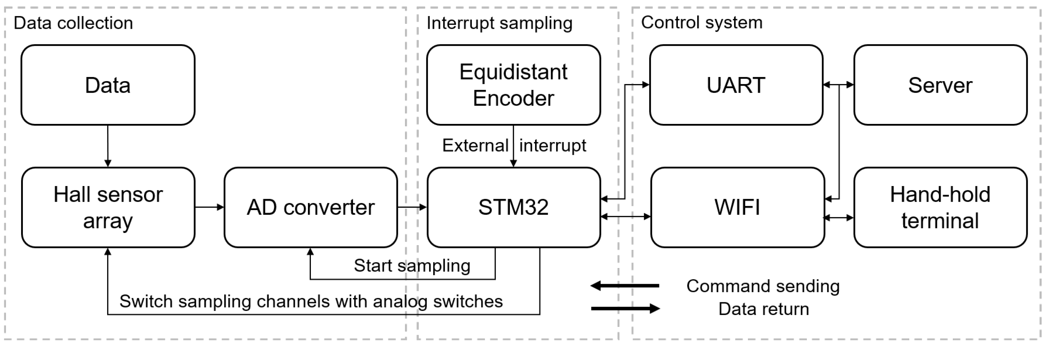
Figure 10.
Experimental diagram (a) Photographic view of the steel wire rope (b) Typical LF defect diagram (c) Typical LMA defect diagram.
Figure 10.
Experimental diagram (a) Photographic view of the steel wire rope (b) Typical LF defect diagram (c) Typical LMA defect diagram.
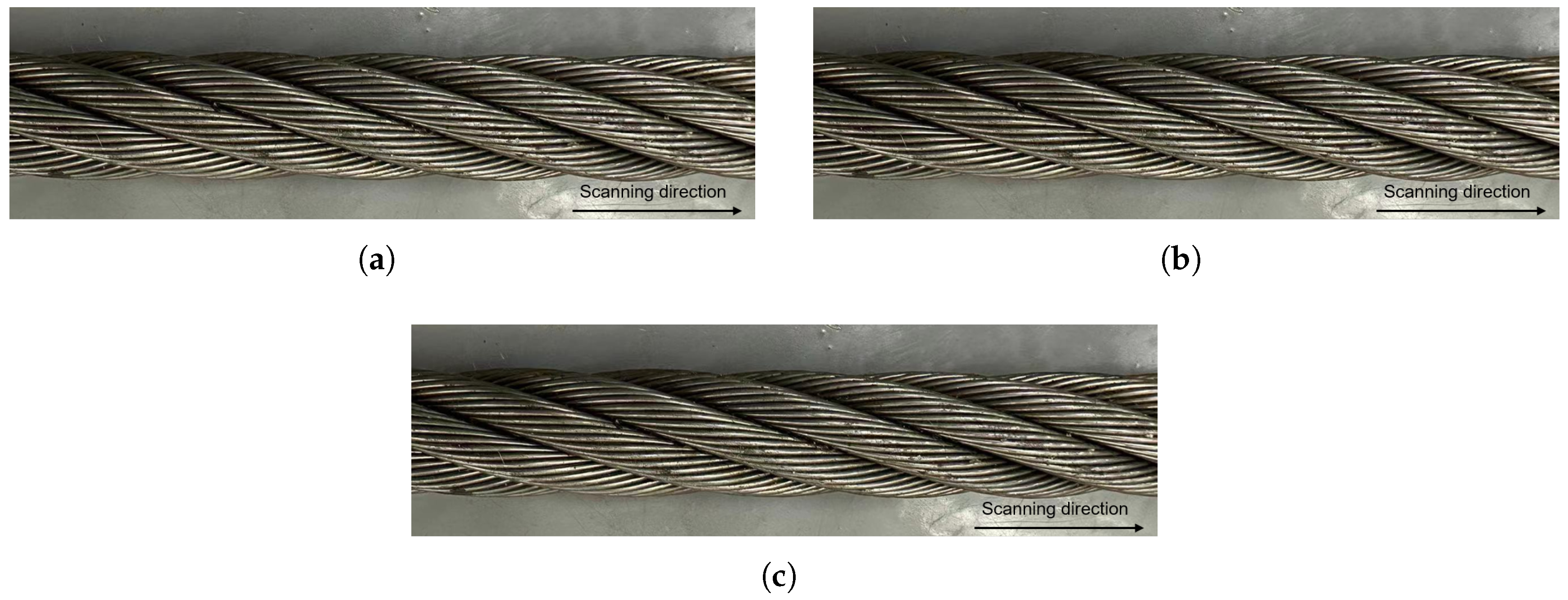
Figure 11.
Typical 3D MFL images (a) Schematic diagram of MFL image (b) Raw MFL image (c) Processed MFL image.
Figure 11.
Typical 3D MFL images (a) Schematic diagram of MFL image (b) Raw MFL image (c) Processed MFL image.
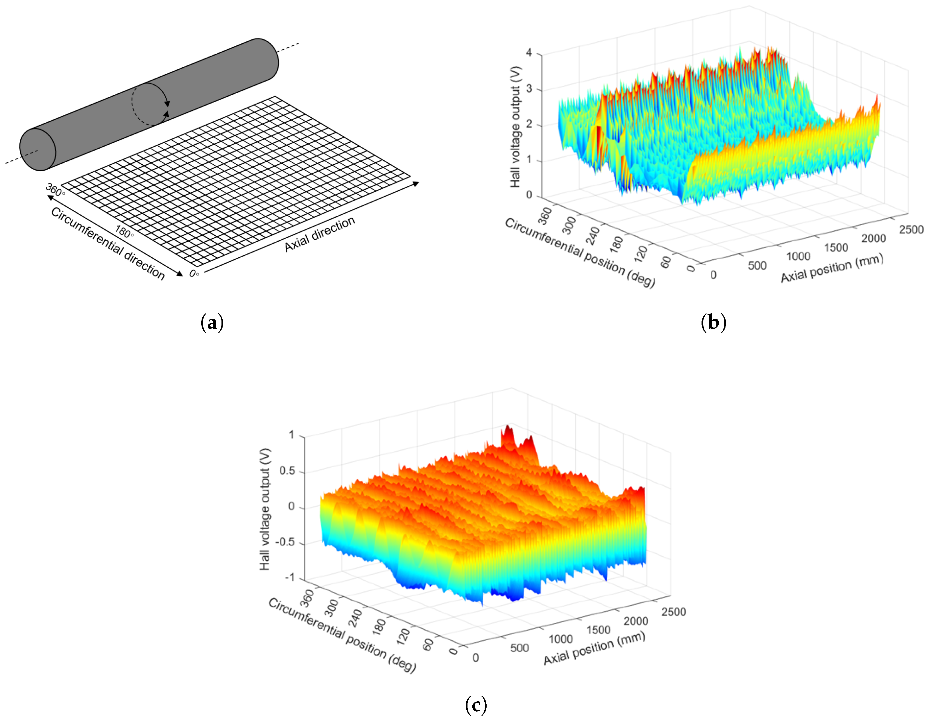
Figure 12.
Typical 2D MFL images (a) MFL image without defect (b) MFL image with defects (c) Texture-Removed MFL image without defect (d) Texture-Removed MFL image with defects.
Figure 12.
Typical 2D MFL images (a) MFL image without defect (b) MFL image with defects (c) Texture-Removed MFL image without defect (d) Texture-Removed MFL image with defects.
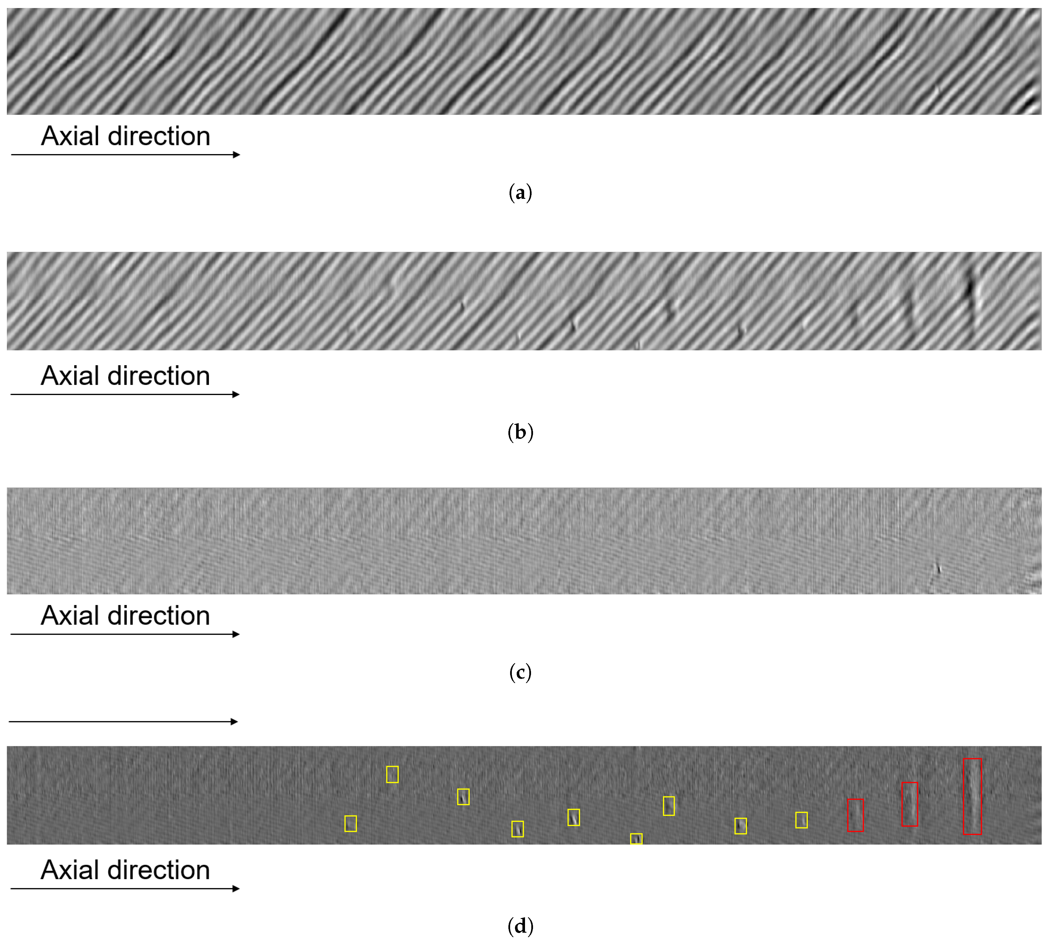
Figure 13.
2D MFL images experimental results (a) prediction result of a MFL image with defects (b) confusion matrix of all the prediction results (c) mAP, Precision, and Recall results.
Figure 13.
2D MFL images experimental results (a) prediction result of a MFL image with defects (b) confusion matrix of all the prediction results (c) mAP, Precision, and Recall results.
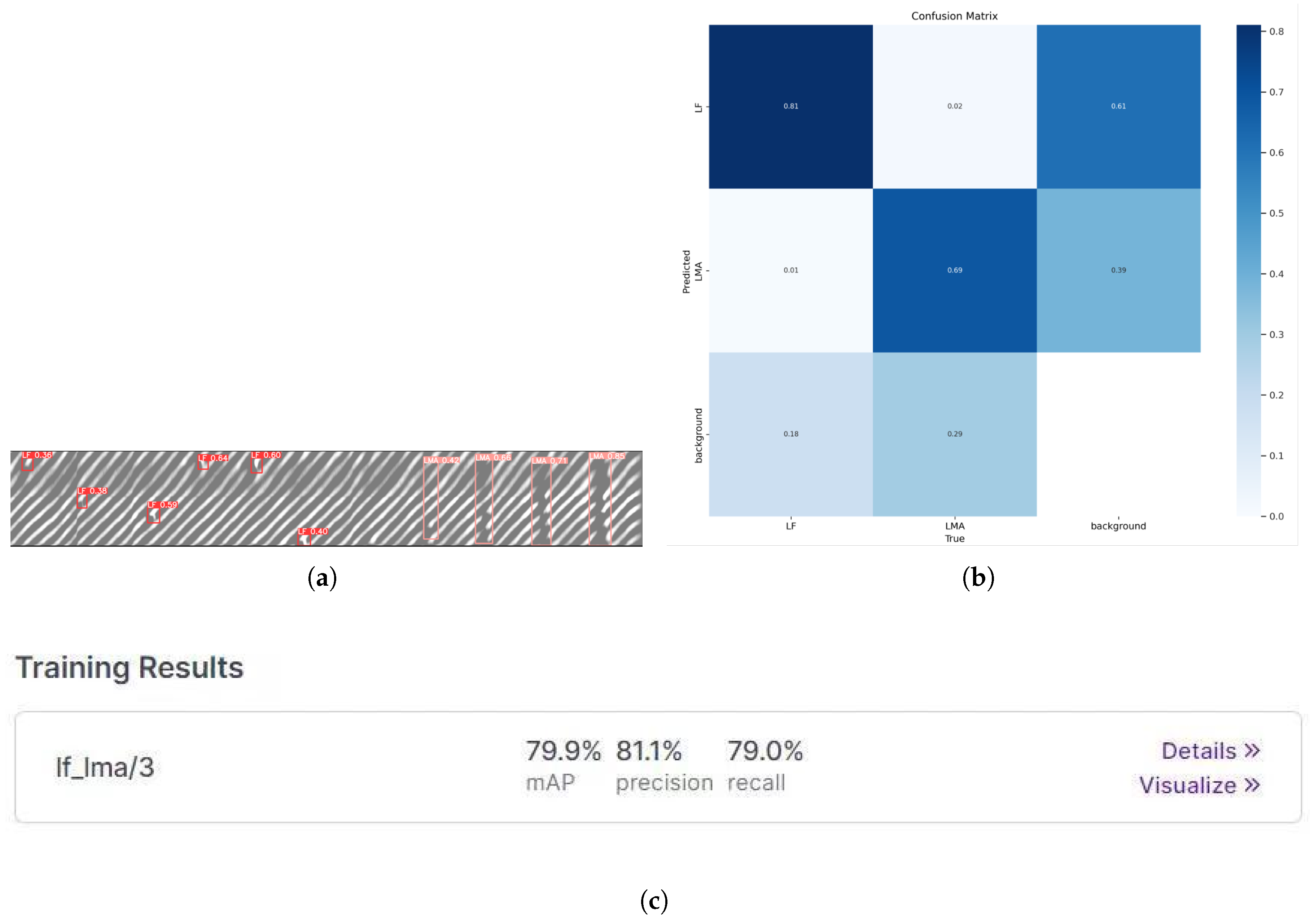

Table 1.
The settings for the training hyperparameters.
| Hyperparameters | Value |
|---|---|
| lr | 0.001 |
| momentum | 0.9 |
| weight_decay | 0.0005 |
| batch_size | 16 |
Disclaimer/Publisher’s Note: The statements, opinions and data contained in all publications are solely those of the individual author(s) and contributor(s) and not of MDPI and/or the editor(s). MDPI and/or the editor(s) disclaim responsibility for any injury to people or property resulting from any ideas, methods, instructions or products referred to in the content. |
© 2025 by the authors. Licensee MDPI, Basel, Switzerland. This article is an open access article distributed under the terms and conditions of the Creative Commons Attribution (CC BY) license (http://creativecommons.org/licenses/by/4.0/).
Copyright: This open access article is published under a Creative Commons CC BY 4.0 license, which permit the free download, distribution, and reuse, provided that the author and preprint are cited in any reuse.


