
Submitted:
13 March 2025
Posted:
14 March 2025
You are already at the latest version
Abstract
Given the growing need to enhance the accuracy of exploration robots, this study focuses on designing a teleoperated navigation system for a robot equipped with a continuous track traction system. The goal is to improve navigation performance by developing mathematical models that describe the robot’s behavior, which are validated through experimental measurements. The system incorporates a digital twin based on ROS (Robot Operating System) to configure the nodes responsible for teleoperated navigation. A PID controller is implemented for each motor, with pole cancellation to achieve first-order dynamics and anti-windup to prevent integral error accumulation when the reference is not met. Finally, a physical implementation is carried out to validate the functionality of the proposed navigation system. The results demonstrate that the system ensures precise and stable navigation, highlighting the effectiveness of the proposed approach in dynamic environments. This work contributes to advancing robotic navigation in controlled environments and offers potential for improving teleoperation systems in more complex scenarios.
Keywords:
Navigation system
; ROS
; remote control
; kinematic model
; dynamic model
; mathematical model
1. Introduction
Robotics has managed to capture the attention of society with its scientific advancements, making it a part of everyday life in many ways. Moreover, it is experiencing tremendous growth due to the integration of sensors, electronics, and software, bringing groundbreaking changes in industries and processes such as mining, transportation, agriculture, etc [1].
This study case is framed in the field of mobile robotics, which meets the need to limit human intervention and facilitate production processes by implementing optimal navigation. This is achieved through mechatronic devices that allow the robot to move in its environment using limbs, wheels or tracks [2].
The morphology of the robot to be controlled is of differential type, a design in which most of the propulsion systems use wheels. From this scheme, the kinematic models of the system are developed, as described in [3,4,5,6,7,8]. For the study case in which the robot has caterpillar tracks, it is important to take into account that the tangential velocity of the caterpillar track is uniform. Therefore, gear ratios are generated in the driving elements of the system, so that the kinematic analysis of the robot can be performed with any element that is part of the track [9,10,11,12].
For the operation of a navigation system, it is important to model all the loads (i.e., forces or moments) acting on the robot to produce its motion. For this purpose, we can use the Lagrange–Euler formulation [13], or the Newton-Euler method [14].
The proposed kinematic and dynamic models are essential to understand the operation of the robot, providing the necessary calculations and equations to develop the navigation system. This process begins with the programming of nodes for teleoperated navigation using ROS, a flexible framework for robotic software development. ROS offers a wide range of tools and libraries for building complex robotic systems and supports multiple programming languages, such as Java, C++ and Python. For teleoperated navigation, it is sufficient to use nodes and topics in ROS. The transmission methods for communicating nodes and topics are described in [15]. A subscriber node then receives these velocity values, which dictate the motion of the robot.
To evaluate programming nodes, ROS-compatible simulation software like Gazebo can be utilized. Gazebo is an open-source platform comprising libraries designed to streamline the development of high-performance robotic applications. It enables the simulation and evaluation of various navigation systems, including teleoperated navigation showed in [16,17], and more advanced systems such as autonomous navigation [18]. Autonomous systems often incorporate a broader range of sensors and tools, such as artificial vision cameras and neural networks, which can be seamlessly implemented within Gazebo.
The ROS topics and nodes must transmit reference values to the system’s actuators, making a control system essential to ensure the robot achieves the commanded speeds. To achieve this, the mathematical model of the controlled systems is required. In this case, the focus is on DC motors with permanent magnets, whose equations and physical principles are detailed in [19,20,21,22]. Additionally, manufacturer data, combined with experimental tests, are used to determine specific system parameters. This process results in the derivation of the motors’ transfer function, which corresponds to a second-order underdamped system.
The mathematical model of the system to be controlled plays a crucial role in facilitating the design of an appropriate controller, especially when analytical techniques are applied. Techniques such as those detailed in [23] and [24] provide a foundation through classical control methods, including PID and Lead-Lag compensators, as well as modern approaches using state-space representations. For more complex systems, advanced methods like fuzzy logic [25] or neural networks [26] can be employed. The selection of a specific control method depends on the system’s complexity and the performance requirements of the desired response.
One of the most commonly used controllers in mobile robot control is the PID controller and its variants [27,28,29], due to its ability to meet the requirements for efficient and precise navigation in such systems. The tuning methods applied to this controller are diverse, ranging from analytical approaches of varying complexity levels [30,31,32], which often incorporate additional techniques such as anti-windup to mitigate the accumulation of the error integral [33,34], to advanced methods that utilize specialized algorithms to achieve optimal controller configuration or more advanced variants of the same [35,36,37].
This work aims to develop a remote navigation system for a differential mobile robot with crawler-type traction. To achieve this, a digital twin is implemented in ROS, enabling the evaluation and optimization of the programmed nodes. The system control is performed using a PID controller, analytically tuned using the pole-zero cancellation technique previously described. Additionally, the control system is evaluated in MATLAB/Simulink to ensure a comprehensive analysis and thorough validation of performance. Finally, the system is tested under real-world conditions, implementing navigation through a Jetson Nano, where all necessary nodes are programmed and configured, and an Arduino Mega 2560, which integrates the motor control system.
2. Materials and Methods
2.1. Establishment of Parameters
The parameters required for the design of the navigation system are obtained from mathematical models, experimental data, data sheets, and data obtained from the mechanical design of the system. The initial parameters, given by the mechanical design and the data sheets, are shown in Table 1.
2.1.1. Robot Kinematic Model
Since the robot operates on a differential drive system, the control variables, V (linear velocity) and (angular velocity), are defined by Equations (2) and (3). These are expressed as functions of the track velocities, which in turn depend on the angular velocity of the driving elements, specifically, the drive sprockets of each track. These sprockets are connected to their respective motors via a transmission ratio i, as defined by Equation (4).
2.1.2. Dynamic Model of the Robot
For the validation of the control system, it is essential to have the model of the forces and moments acting on the robot, as these serve as disturbances to the control system, enabling the evaluation of the system’s robustness. Newton’s equations are applied to the dynamic model, based on the equilibrium diagrams presented in Figure 2.
If Newton’s second law for rotational mechanics is applied using the moments generated by the forces from Figure 2, the Equation is obtained.
2.1.3. Parameters for the Control System
The kinematic and dynamic models describe the robot’s behavior, providing information on key parameters for the navigation system. However, it must be considered that the response of the actuators is not ideal, so obtaining their transfer function is essential to design a control system and ensure that the system reaches the desired reference values. To this end, experimental tests are conducted to approximate the transfer functions, which are given by Equation (13) for the right motor and by Equation (14) for the left motor.
The models previously shown correspond to a second-order underdamped system, with each model having an equivalent circuit like the one in Figure 3, and they are governed by Kirchhoff’s laws, as shown in Equation (15), and by Newton’s second law in Equation (16).
Equation (16) can be rewritten as a difference between the torque delivered by the motor, which is given by Equation (17), and the disturbance torques modeled by Equations (11) and (12).
With these equations and the block diagram corresponding to the motor in Figure 4, a simulation of the entire system can be performed, allowing the evaluation of the controller’s behavior when subjected to different disturbances modeled by the load torque Td.
2.2. Design Proposal
For the navigation of the robot, a remote control is used that is connected to a computer designated as “Master”. This computer publishes the velocities at which the robot must move in the topical cmd_vel. This topic, in turn, sends these values to the node controlling the motors in the robot’s CPU. Using Equations (5) and (6), the angular velocities of the robot’s motors are calculated and these reference values are sent to the control system at each time instant. The detailed scheme of this process is shown in Figure 5.
2.2.1. Programming the Robot in ROS
For the robot programming, the teleop_twist_joy package was used to configure the controller shown in Figure 6.
The installed node allows configuring the buttons and axes from Figure 6 and scaling them to the robot’s velocity values obtained in Table 2, so that the node publishes the robot’s linear velocity V and angular velocity on the cmd_vel topic.
On the other hand, for the implementation of the digital twin in Gazebo, the URDF file of a simplified version of the robot is used, where the robot’s masses shown in Table 1 are configured. Additionally, the differential_drive_controller plugin is added, in which the angular velocities, angular accelerations, and torques of the driving wheels are configured using the data from Table 1 and Table 2. In this way, the connection of the nodes with the velocity topic is as shown in Figure 7.
2.2.2. Design of the Control System
To ensure that the motors’ acceleration does not produce torques greater than previously stated, a response time is proposed that depends on this parameter and the maximum angular velocity.
Using Equation (19), a response time of 0.322 s is obtained, so the pole dominating the dynamics of both systems must be located at 12.4224. To achieve this, a PID controller is proposed, with a transfer function for each motor, as shown in Equation (20).
The PID controller is designed in such a way that the dynamics of the plant to be controlled are nullified, so that, in a closed loop, the system has a first-order transfer function used te pole-zero cancelation. In this way, the desired response time can be controlled almost freely. However, controllers that employ an integrative part to correct the steady-state error have a drawback: when the control signal saturates, which is inevitable in physical systems, the integral of the error begins to accumulate over time, leading to the windup effect. Therefore, it is necessary to counteract this effect with some anti-windup technique, such as those discussed before.
On the other hand, the mathematical models of the plants are second-order underdamped, as shown in Equation (21).
Pole cancellation nullifies the plant’s dynamics, ensuring that Equation (22) is satisfied.
In this way, the direct chain of the system is given by Equation (23).
Therefore, considering unit feedback as shown in the diagram of Figure 8, the closed-loop transfer function is given by Equation (24).
With the response time equation for a first-order system, Equation 25 is obtained.
Equations (22) and (25) allow finding the values of the PID controllers that adjust the response to the desired time and eliminate the steady-state error. These values are shown in Table 5.
With the controller designed and functional in continuous time, a control algorithm can be obtained, making use of numerical methods to go from the complex domain s to the complex domain z. The complexity of the methods varies according to the precision and accuracy desired in the estimation; some of the best-known methods can be seen in [39]. For the discretization of the controllers, the Backward Euler method is used, with a sampling time of 25 ms. This time was determined analytically, considering the smallest sampling interval allowed by the encoders of the motors used. In this way, the necessary equations for the control algorithms are obtained, as shown below.
Equations (26) and (28) correspond to the control laws for the right and left motors, respectively, while Equations (27) and (29) correspond to the equations for the error integrals of both motors, in which the anti-windup technique shown in Figure 9 is applied.
For the physical implementation, the joy_node and teleop_node, shown in Figure 7, are programmed in ROS, installed on a Linux-based operating system (Ubuntu 20.04) on a computer designated as the master. On the other hand, the computer responsible for receiving commands from the master computer, known as the slave, does not require node programming, as it will only connect to the master via a network. This computer, also equipped with ROS and the same operating system, is a Jetson Nano. Its primary function is to transmit the received velocities to the control system via serial communication, maintaining the structure outlined in Figure 5.
Finally, the control system is implemented on a microcontroller, specifically on an Arduino Mega 2560, using ROS libraries to manage communication with the topics sent by the master computer’s nodes. Based on the robot’s linear and angular velocity values received through the cmd_vel topic, individual references for each motor are calculated using the robot’s kinematic model. These references are subsequently sent to the discretized PID controller, equipped with an anti-windup system to ensure a quick response under saturation conditions.
3. Results
3.1. Implementation of ROS Nodes in Gazebo
The nodes programmed in ROS are evaluated through the implementation of the digital twin in Gazebo, using two network-connected computers: the master, with the nodes to read the controller values and publish them as velocity values, and the slave, with the Gazebo node running to simulate the physical movement of the robot based on the received velocity commands. In this way, the topic is published by the master computer, while the same topic is read and processed by the slave computer.
3.2. Simulation of the Control System
Before implementing the control system with the mathematical models of the robot, it was verified that the performance of the controllers tuned using the pole-zero cancellation method met the established design conditions. To achieve this, the control system’s response for both the right motor and the left motor was evaluated in continuous time, obtaining an output curve in response to a step input, as shown in Figure 11.
The response shape shown in Figure 11 corresponds to the curve of the left motor. However, since the tuning method used for both motors is exactly the same, the right motor’s response exhibits an identical shape. When the control system is discretized and its behavior is analyzed in response to a step input, the resulting curve is shown in Figure 12.
Similarly to the previous case, the curve shown in Figure 12 corresponds to the left motor, while the curve for the right motor is practically identical. Additionally, as observed in both figures, the behavior of the two systems is similar, with a slight discrepancy around 0.4 seconds. At that point, the discrete system deviates from behaving like a first-order system, exhibiting a small overshoot that is negligible. This difference is more clearly seen in Figure 13.
The discrepancy between the responses in continuous and discrete time arises because, when discretizing the continuous system, pure integrations and differentiations disappear. Additionally, the numerical method used for discretization plays a crucial role in determining how well the discrete-time system approximates the continuous-time system.
Another fundamental factor in the discretization of the control system is the sampling time. Regardless of the numerical method used, a shorter sampling interval ensures a better approximation to the continuous-time system. In the case of Figure 13, the discrete-time system demonstrates good performance using the Backward Euler method with a sampling period of 25 ms.
When a saturator is implemented in the previously evaluated control system, the behavior of the response changes dramatically. When the system operates without the anti-windup controller and a saturator, its behavior is shown in Figure 14. During saturation, when the actuators reach their maximum speed limit, they are unable to precisely track the reference velocity, causing a delay in the system’s response. This delay arises because the controller’s integrative part continues to accumulate error as the reference is not reached. Once the system returns to its operational limits, the output signal remains unchanged until the integral is fully discharged. It is crucial to note that even when the control signal is saturated, if the integral continues to grow, the control signal will stay at its saturation limit until the integral is entirely cleared.
To solve this problem, an anti-windup controller is implemented. This controller limits the accumulation of error over time, preventing the error from increasing indefinitely while the system is saturated. Thanks to this controller, when the system exits saturation and returns to its operational limits, the actual velocity quickly adjusts to follow the reference velocity instantaneously, eliminating the delay and improving the system’s response accuracy, as shown in Figure 15. The same controller has been applied to the right motor, ensuring the system operates correctly.
As observed in Figure 15, when the system is saturated, it does not reach the desired value because the control signal can no longer grow to adequately follow the reference. Additionally, this saturation alters the system’s behavior whenever the controller calculates a control signal greater than the saturation limit.
The desired behavior, as shown in Figure 12, will only be achieved if the control signal sent to the actuator always corresponds to the signal calculated by the controller. Otherwise, if saturation persists, even for a short period of time, the desired behavior of a first-order system can be lost. As shown between 6 and 7 seconds in Figure 15, the system exhibits under damped second-order behavior.
Finally, the system was validated using all the mathematical models, aiming to achieve responses as close as possible to those of a physical system. The simulated system is shown in Figure 16.
The system shown in Figure 16 consists of three fundamental blocks. The first is the controller, which implements the algorithms described in Figure 10 for both motors. Using step inputs for linear and angular velocities, connected to sliders, reference velocities are sent to the robot. Equations (5) and (6) are used to calculate the reference velocities for the motors.
The second block is the actuator, which contains the block diagram shown in Figure 4, where the inputs are the control signal and the disturbance torque. Lastly, the robot block includes kinematic and dynamic models, which allow the generation of graphs showing the linear and angular velocities achieved by the robot. Additionally, the dynamic model provides feedback to the actuators with the load torque generated by the robot.
With the system in operation, the linear velocity graphs, shown in Figure 17, and the angular velocity graphs, shown in Figure 18, are obtained, where the reference velocities are compared with the actual velocities.
The behavior of the curves in Figure 17 and Figure 18 is due to the saturation or physical limitation of the actuators, which have a maximum angular velocity of 321.6 rad/s. When a combination of linear and angular velocity is presented simultaneously, according to Equations (5) and (6), one of the two motors, depending on the direction of the robot’s movement, will need to exceed its maximum speed to reach the reference values. Since the system cannot achieve this, a steady-state error is generated. Additionally, the load that the motors must overcome reduces their maximum angular velocity, causing the saturation to occur sooner. When the linear velocity is saturated and the reference angular velocity changes, the linear velocity deviates from its reference to try to compensate for the angular velocity, similarly, when the angular velocity is saturated and the linear velocity changes. This effect is evident between 12 and 25 seconds of the simulation. Likewise, when the system exits saturation and returns to its operational limits, the anti-windup controller allows the output signal to quickly follow the reference, as observed around 35 seconds.
3.3. Implementation of the Navigation System
Once the systems were validated through simulation, they were physically implemented using the Jetson Nano and the Arduino Mega 2560. At this stage, the control system’s performance was initially evaluated by applying a constant reference value for linear velocity, followed by a constant reference value for angular velocity. The results obtained demonstrated that the system’s responses meet the established requirements. Figure 19 shows the graphs of the reference signal and the measured signal for linear velocity, while Figure 20 presents the corresponding graphs for angular velocity.
The horizontal axis of both graphs indicates the number of samples taken at regular intervals of 25 milliseconds, corresponding to the sampling time. This means that every 100 samples represent a 2.5-second interval. It can be observed that the process signal reaches the reference value around sample 15, which is approximately 0.375 seconds. Furthermore, as shown in the figures, the steady-state error is zero, demonstrating the correct performance of the system.
With the control system operating correctly, the master computer nodes were activated, and the serial connection between the Arduino and the Jetson Nano was established. From the Arduino code, the most relevant data was published on a new topic named w_m, which maintains the same structure as the cmd_vel topic. In this topic, the components x, y y z correspond to the control signal, the reference motor velocity, and the measured motor velocity, respectively. It is important to highlight that the linear velocity components are associated with the left motor, while the angular velocity components correspond to the right motor, as shown in Figure 21.
4. Conclusions
The acquisition of the robot’s parameters from mathematical models, datasheets, and mechanical design specifications is a crucial aspect, as these serve as input variables for designing the navigation system. In this work, three main stages were addressed: programming in ROS, controller design, and physical implementation. Programming the robot using ROS enabled the networking of a digital twin of the robot simulated on a computer with another computer used to control the system’s navigation via a remote control with joysticks.
On the other hand, the selected PID controller met all the established requirements, demonstrating optimal performance in the system simulated in MATLAB/SIMULINK. In this simulation, the most relevant parameters were considered to make the system resemble a real system as closely as possible, taking into account physical limitations such as the operational range of the actuators. To address these constraints, solutions such as the anti-windup compensator were proposed, designed to prevent excessive error accumulation.
Finally, the physical implementation of the navigation system allowed for the validation of both the performance of the programmed nodes and the designed control system. These components were seamlessly integrated with the physical equipment that will operate the robot, demonstrating the proper functioning of its remote navigation.
Author Contributions
Study conception and design, M.A., A.U., D.A., J.V., and J.L.; data collection, D.A., A.U. and J.V.; software A.U., D.A. and J.V.; Methodology, A.U., D.A. and J.V.; analysis and interpretation of results, M.A., A.U., D.A., J.V., J.L. and L.L.; writing—original draft preparation, A.U., D.A. and J.V.; writing—review and editing, L.L. All authors have read and agreed to the published version of the manuscript.
Funding
This research was funded by Universidad Politécnica Salesiana.
Institutional Review Board Statement
Not applicable.
Data Availability Statement
Data will be made available on request.
Conflicts of Interest
The authors declare no conflicts of interest.
References
- Baturone, A. Robótica: manipuladores y robots móviles; Marcombo, 2005; p. 1. [Google Scholar]
- Raj, R.; Kos, A. A Comprehensive Study of Mobile Robot: History, Developments, Applications, and Future Research Perspectives. Applied Sciences 2022, 12. [Google Scholar] [CrossRef]
- VALENCIA V., J.A.; MONTOYA O., A.; RIOS, L.H. MODELO CINEMÁTICO DE UN ROBOT MÓVIL TIPO DIFERENCIAL Y NAVEGACIÓN A PARTIR DE LA ESTIMACIÓN ODOMÉTRICA. Scientia Et Technica 2009.
- Feng, S.; Liu, Y.; Pressgrove, I.; Ben-Tzvi, P. Autonomous Alignment and Docking Control for a Self-Reconfigurable Modular Mobile Robotic System. Robotics 2024, 13. [Google Scholar] [CrossRef]
- Chen, X.; Jia, Y.; Matsuno, F. Tracking control for differential-drive mobile robots with diamond-shaped input constraints. IEEE Transactions on Control Systems Technology 2014, 22, 1999–2006. [Google Scholar] [CrossRef]
- Giorgi, C.D.; Palma, D.D.; Parlangeli, G. Online Odometry Calibration for Differential Drive Mobile Robots in Low Traction Conditions with Slippage. Robotics 2024, 13. [Google Scholar] [CrossRef]
- Kouvakas, N.D.; Koumboulis, F.N.; Sigalas, J. A Two Stage Nonlinear I/O Decoupling and Partially Wireless Controller for Differential Drive Mobile Robots. Robotics 2024, 13. [Google Scholar] [CrossRef]
- He, S. Feedback control design of differential-drive wheeled mobile robots. In Proceedings of the ICAR ’05. Proceedings., 12th International Conference on Advanced Robotics, 2005., 2005, pp. 135–140. [CrossRef]
- Sotelo Gomez, A.A. Implementación de un robot explorador con realidad virtual para incrementar la seguridad de la Institución Educativa 7213 Peruano Japonés en el distrito de Villa El Salvador–2020. Licenciatura thesis, Universidad Privada del Norte, 2020.
- Martinez, J.; Mandow, A.; Morales, J.; Garcia-Cerezo, A.; Pedraza, S. Kinematic modelling of tracked vehicles by experimental identification. In Proceedings of the 2004 IEEE/RSJ International Conference on Intelligent Robots and Systems (IROS) (IEEE Cat. No.04CH37566), 2004, Vol. 2, pp. 1487–1492 vol.2. [CrossRef]
- moosavian, S.A.A.; Kalantari, A. Experimental Slip Estimation for Exact Kinematics Modelling and Control of a Tracked Mobile Robot. 2008 IEEE/RSJ International Conference on Intelligent Robots and Systems 2008. [CrossRef]
- Iossaqui, J.G.; Camino, J.F.; Zampieri, D.E. A nonlinear control design for tracked robots with longitudinal slip. In Proceedings of the IFAC Proceedings Volumes (IFAC-PapersOnline). IFAC Secretariat, 2011, Vol. 44, pp. 5932–5937. [CrossRef]
- Choset, H.; Lynch, K.M.; Hutchinson, S.; Kantor, G.A.; Burgard, W. Configuration Space. In Principles of Robot Motion: Theory, Algorithms, and Implementations; MIT Press, 2005; pp. 47–68. [Google Scholar]
- Spong, M.W.; Hutchinson, S.; Vidyasagar, M. DYMAMICS AND MOTION PLANNING. In Robot Modeling and Control, 2nd ed.; John Wiley & Sons, 2020; Vol. 1, pp. 165–214. [Google Scholar]
- Du, K.L.; Swamy, M.N.S. Wireless Communication Systems. Conference Record of 2004 Annual Pulp and Paper Industry Technical Conference (IEEE Cat. No.04CH37523) 2010, pp. 94–101. [CrossRef]
- Blanco Abia, C. Desarrollo de un sistema de navegación para un robot móvil. PhD thesis, Universidad de Valladolid, Escuela de Ingenierías Industriales, 2014.
- Nasirian, A.; Khanesar, M.A. Sliding mode fuzzy rule base bilateral teleoperation control of 2-DOF SCARA system. In Proceedings of the 2016 International Conference on Automatic Control and Dynamic Optimization Techniques (ICACDOT), 2016, pp. 7–12. [CrossRef]
- Lee, C. Fuzzy logic in control systems: fuzzy logic controller. I. IEEE Transactions on Systems, Man, and Cybernetics 1990, 20, 404–418. [CrossRef]
- Chapman, S. Motores y generadores de corriente directa. In Máquinas Eléctricas, 5 ed.; Mc Graw Hill, 2012; pp. 345–413. [Google Scholar]
- Nise, N.S. MODELING IN THE FREQUENCY DOMAIN. In Control Systems Engineering, 8 ed.; John Wiley & Sons, 2020; pp. 33–115. [Google Scholar]
- Stefek, A.; van Pham, T.; Krivanek, V.; Pham, K.L. Energy comparison of controllers used for a differential drive wheeled mobile robot. IEEE Access 2020, 8, 170915–170927. [Google Scholar] [CrossRef]
- Rahayu, E.S.; Ma’arif, A.; Cakan, A. Particle Swarm Optimization (PSO) Tuning of PID Control on DC Motor. International Journal of Robotics and Control Systems 2022, 2, 435–447. [Google Scholar] [CrossRef]
- Nise, N.S. Controller Design. In Control Systems Engineering, 8 ed.; John Wiley & Sons, 2020; pp. 455–721. [Google Scholar]
- Ogata, K. Diseño de controladores. In Ingeniería de control moderna, 5 ed.; Pearson Educación, 2010; pp. 416–745. [Google Scholar]
- Lee, C. Fuzzy logic in control systems: fuzzy logic controller. I. IEEE Transactions on Systems, Man, and Cybernetics 1990, 20, 404–418. [Google Scholar] [CrossRef]
- Sierra-García, J.E.; Santos, M. Redes neuronales y aprendizaje por refuerzo en el control de turbinas eólicas. Revista Iberoamericana de Automática e Informática industrial 2021, 18, 327–335. [Google Scholar] [CrossRef]
- Carlucho, I.; Paula, M.D.; Acosta, G.G. Double Q-PID algorithm for mobile robot control. Expert Systems with Applications 2019, 137, 292–307. [Google Scholar] [CrossRef]
- Bârsan, A. Position Control of a Mobile Robot through PID Controller. Acta Universitatis Cibiniensis. Technical Series 2019, 71, 14–20. [Google Scholar] [CrossRef]
- Padhy, P.K.; Sasaki, T.; Nakamura, S.; Hashimoto, H. Modeling and position control of mobile robot. In Proceedings of the 2010 11th IEEE International Workshop on Advanced Motion Control (AMC). IEEE, 3 2010, pp. 100–105. [CrossRef]
- MSajnekar, D.; scholar Ycce.; Road, H. Comparison of Pole Placement & Pole Zero Cancellation Method for Tuning PID Controller of A Digital Excitation Control System. International Journal of Scientific and Research Publications 2013, 3.
- Kim, K.; Schaefer, R. Tuning a PID controller for a digital excitation control system. In Proceedings of the Conference Record of 2004 Annual Pulp and Paper Industry Technical Conference (IEEE Cat. No.04CH37523). IEEE, 2004, pp. 94–101. [CrossRef]
- Zhang, W.; Cui, Y.; Ding, X. An improved analytical tuning rule of a robust pid controller for integrating systems with time delay based on the multiple dominant pole-placement method. Symmetry 2020, 12. [CrossRef]
- Peng, Y.; Vrancic, D.; Hanus, R. Anti-windup, bumpless, and conditioned transfer techniques for PID controllers. IEEE Control Systems 1996, 16, 48–57. [Google Scholar] [CrossRef]
- Bohn, C.; Atherton, D.P. An analysis package comparing PID anti-windup strategies. IEEE Control Systems 1995, 15, 34–40. [Google Scholar] [CrossRef]
- Gün, A. Attitude control of a quadrotor using PID controller based on differential evolution algorithm. Expert Systems with Applications 2023, 229. [Google Scholar] [CrossRef]
- Mousakazemi, S.M.H.; Ayoobian, N. Robust tuned PID controller with PSO based on two-point kinetic model and adaptive disturbance rejection for a PWR-type reactor. Progress in Nuclear Energy 2019, 111, 183–194. [Google Scholar] [CrossRef]
- Mosaad, A.M.; Attia, M.A.; Abdelaziz, A.Y. Whale optimization algorithm to tune PID and PIDA controllers on AVR system. Ain Shams Engineering Journal 2019, 10, 755–767. [Google Scholar] [CrossRef]
- Jia, W.; Liu, X.; Jia, G.; Zhang, C.; Sun, B. Research on the Prediction Model of Engine Output Torque and Real-Time Estimation of the Road Rolling Resistance Coefficient in Tracked Vehicles. Sensors 2023, 23. [Google Scholar] [CrossRef] [PubMed]
- FunctionBay, I. Discrete Time Integrator, n.d. Accessed: 2024-07-10.
Figure 1.
Location in the plane of a differential mobile robot.
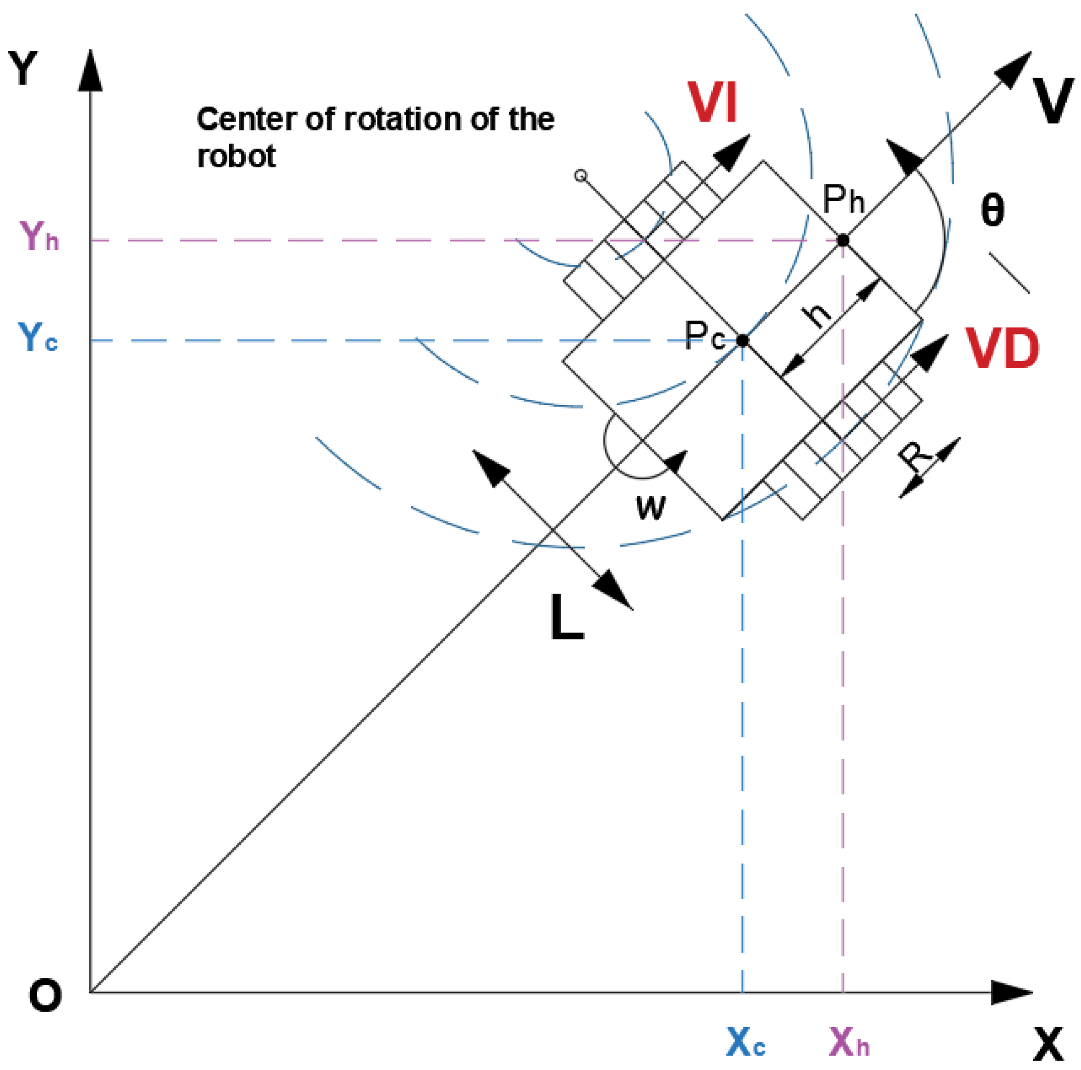
Figure 2.
Equilibrium diagrams for the dynamic model of the differential robot. (a) Equilibrium diagram in the XZ plane. (b) Equilibrium diagram in the XY plane.
Figure 2.
Equilibrium diagrams for the dynamic model of the differential robot. (a) Equilibrium diagram in the XZ plane. (b) Equilibrium diagram in the XY plane.
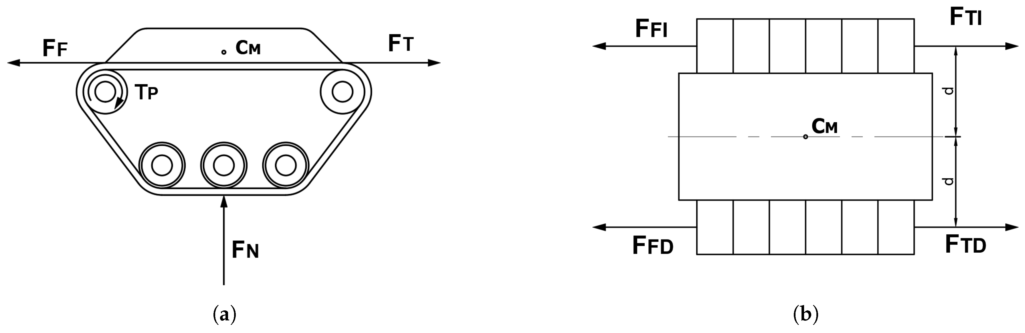
Figure 3.
Equivalent circuit of a permanent magnet DC motor. [20]
Figure 3.
Equivalent circuit of a permanent magnet DC motor. [20]
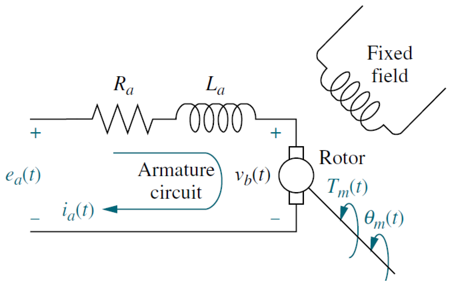
Figure 4.
Mathematical model of a permanent magnet motor with block diagram.
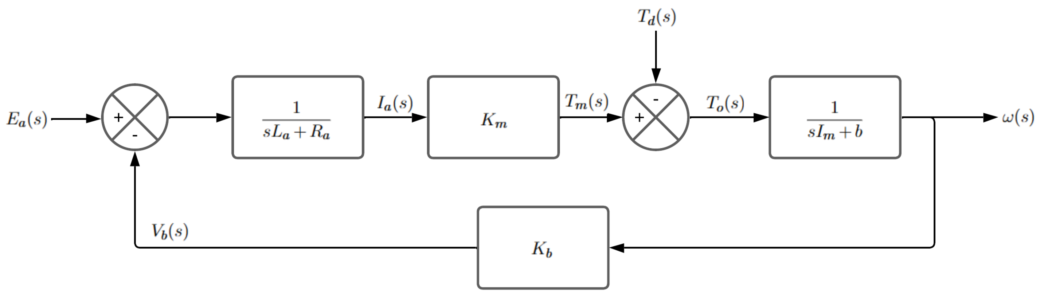
Figure 5.
Schematic of the remote navigation system.
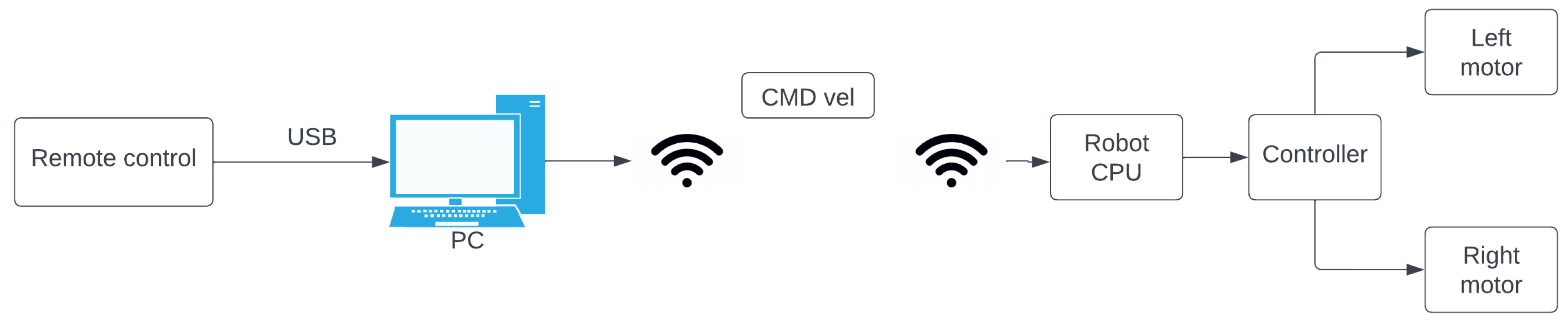
Figure 6.
Physical controller used for the teleoperated navigation of the robot.
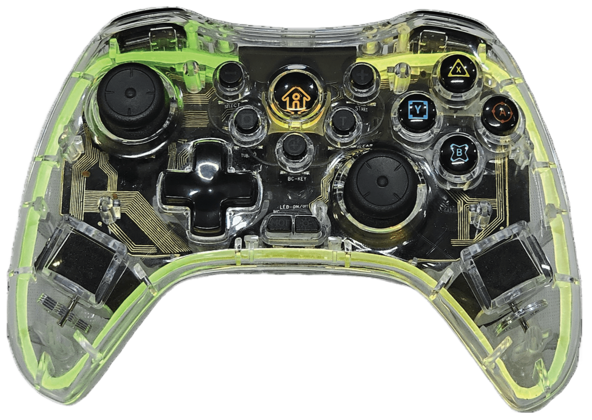
Figure 7.
Schematic of the connection between nodes.
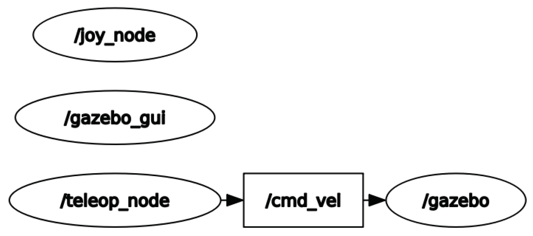
Figure 8.
Schematic of the control system with unity feedback.
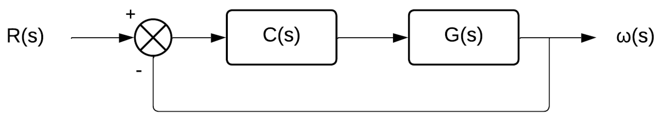
Figure 9.
Schematic of the control system with unity feedback and anti-windup.
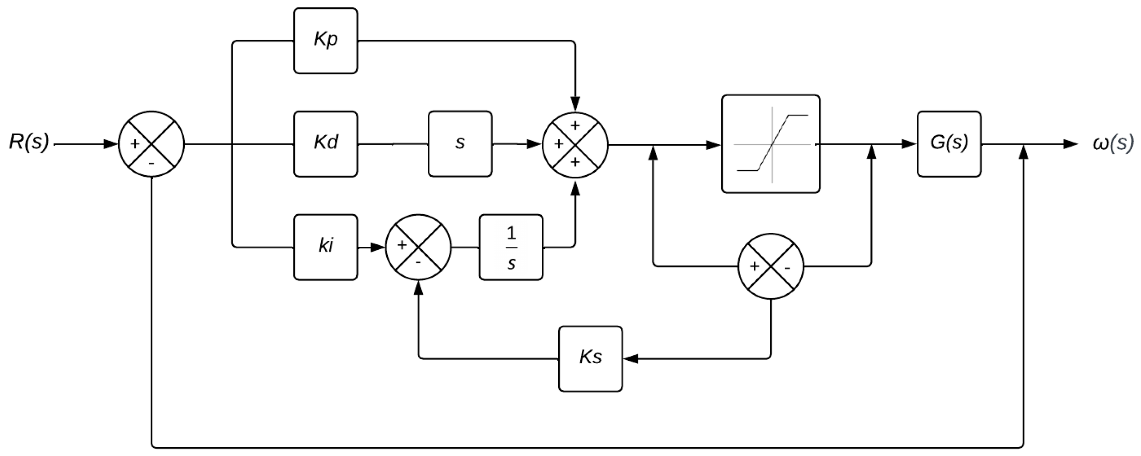
Figure 10.
Schematic of the control system with unity feedback and anti-windup.
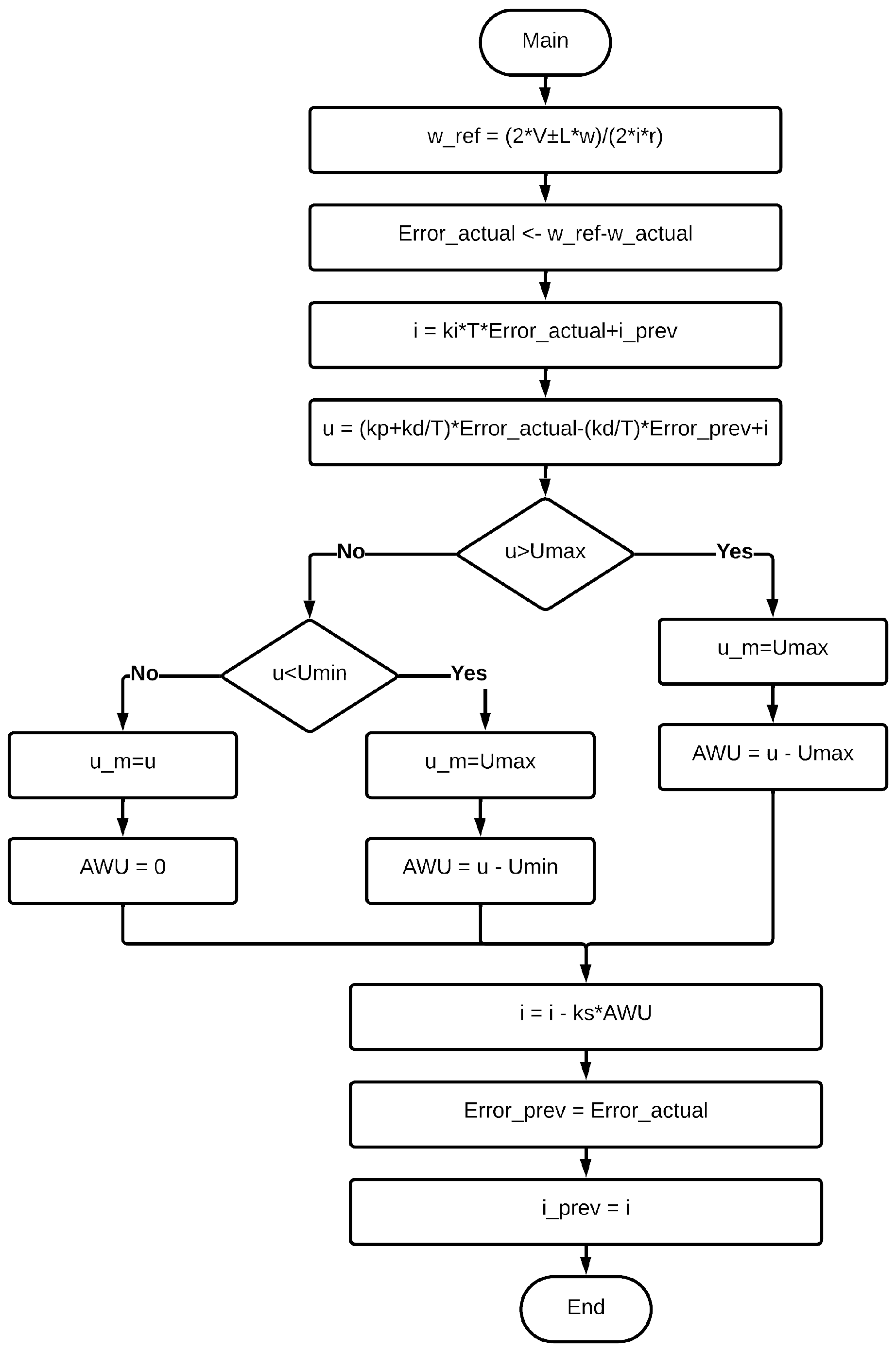
Figure 11.
Performance of the control system for the left motor in response to a step input in continuous time.
Figure 11.
Performance of the control system for the left motor in response to a step input in continuous time.
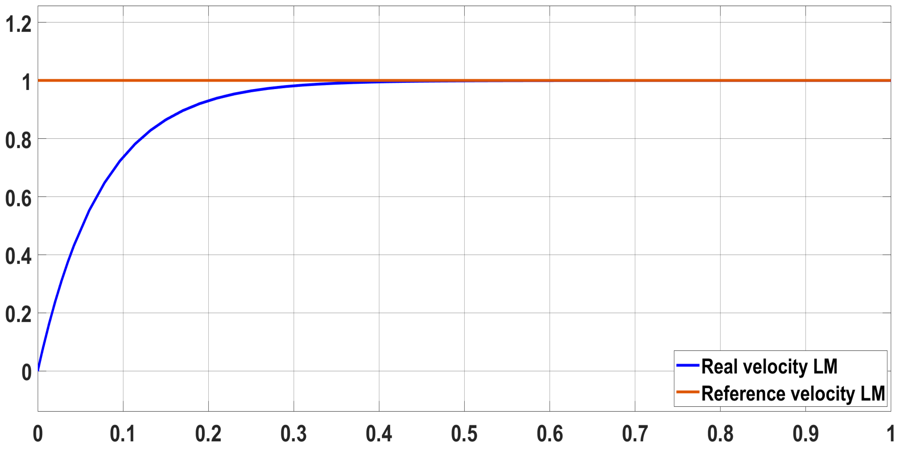
Figure 12.
Performance of the control system for the left motor in response to a step input in discrete time.
Figure 12.
Performance of the control system for the left motor in response to a step input in discrete time.
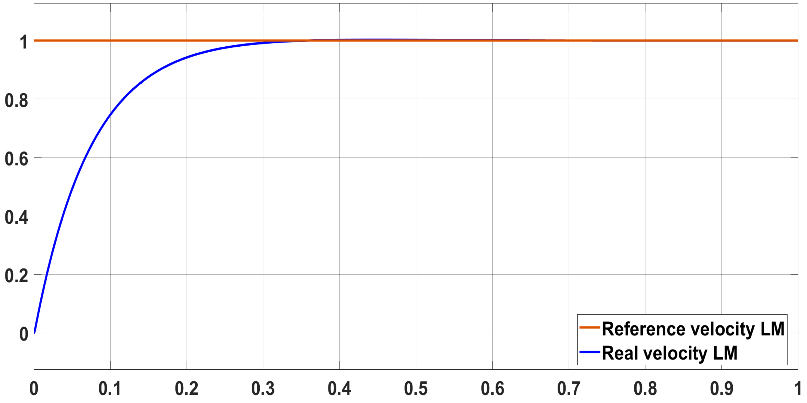
Figure 13.
Comparison between the behavior of the continuous and discrete controllers in response to a step input.
Figure 13.
Comparison between the behavior of the continuous and discrete controllers in response to a step input.
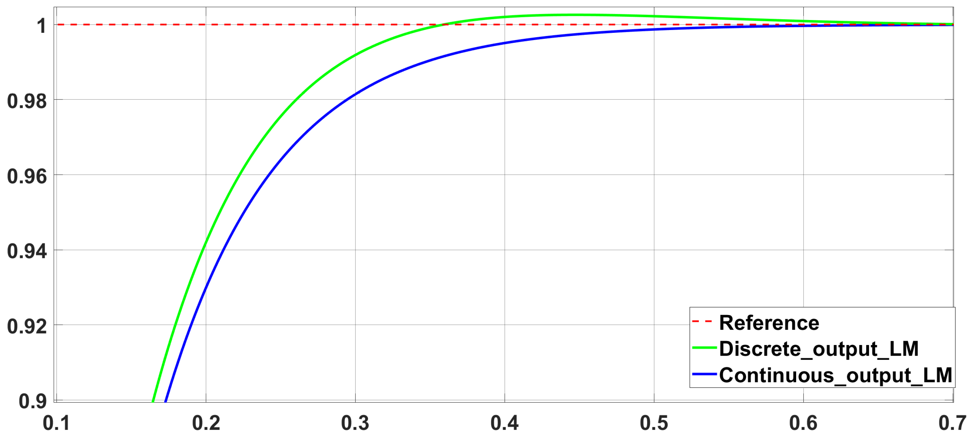
Figure 14.
Windup effect on the left motor.
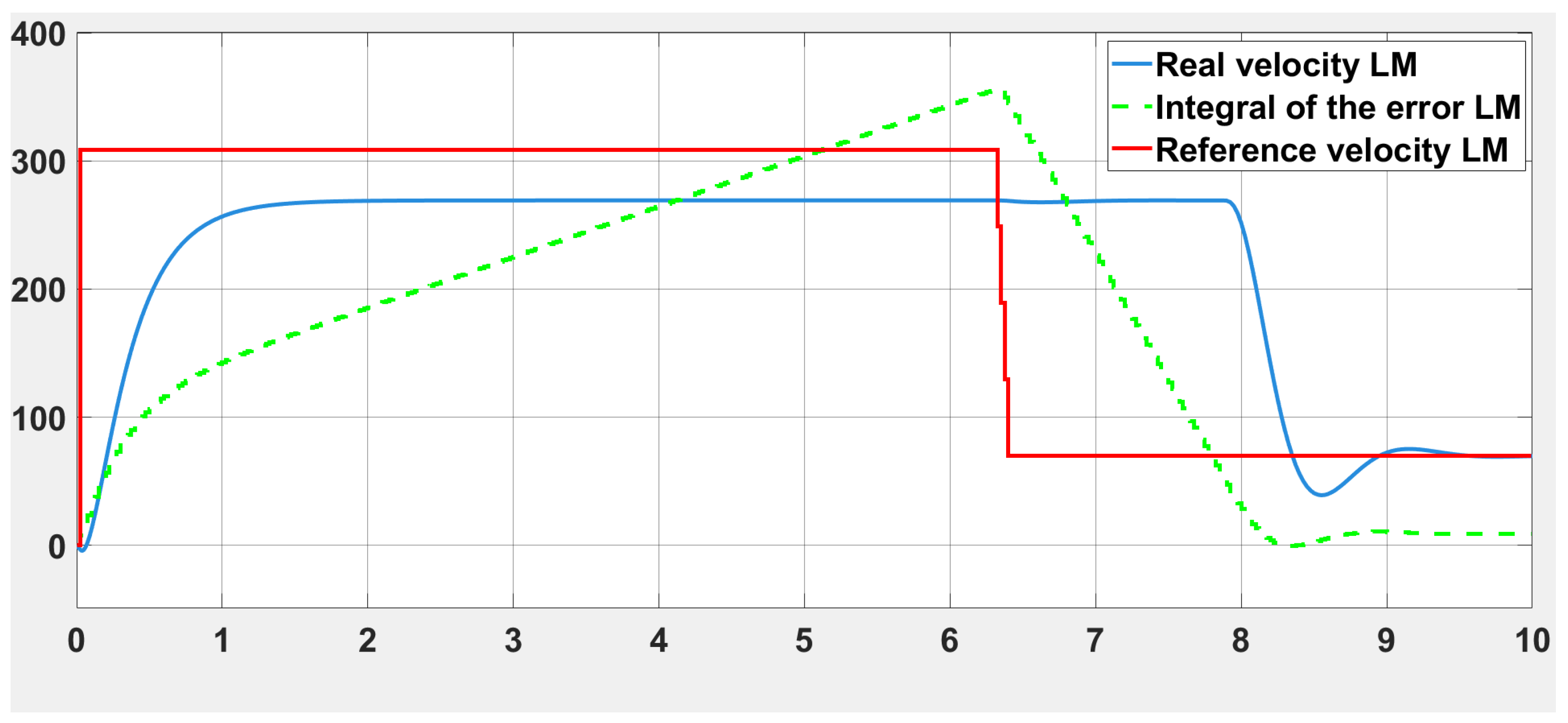
Figure 15.
Anti-windup effect on the left motor.
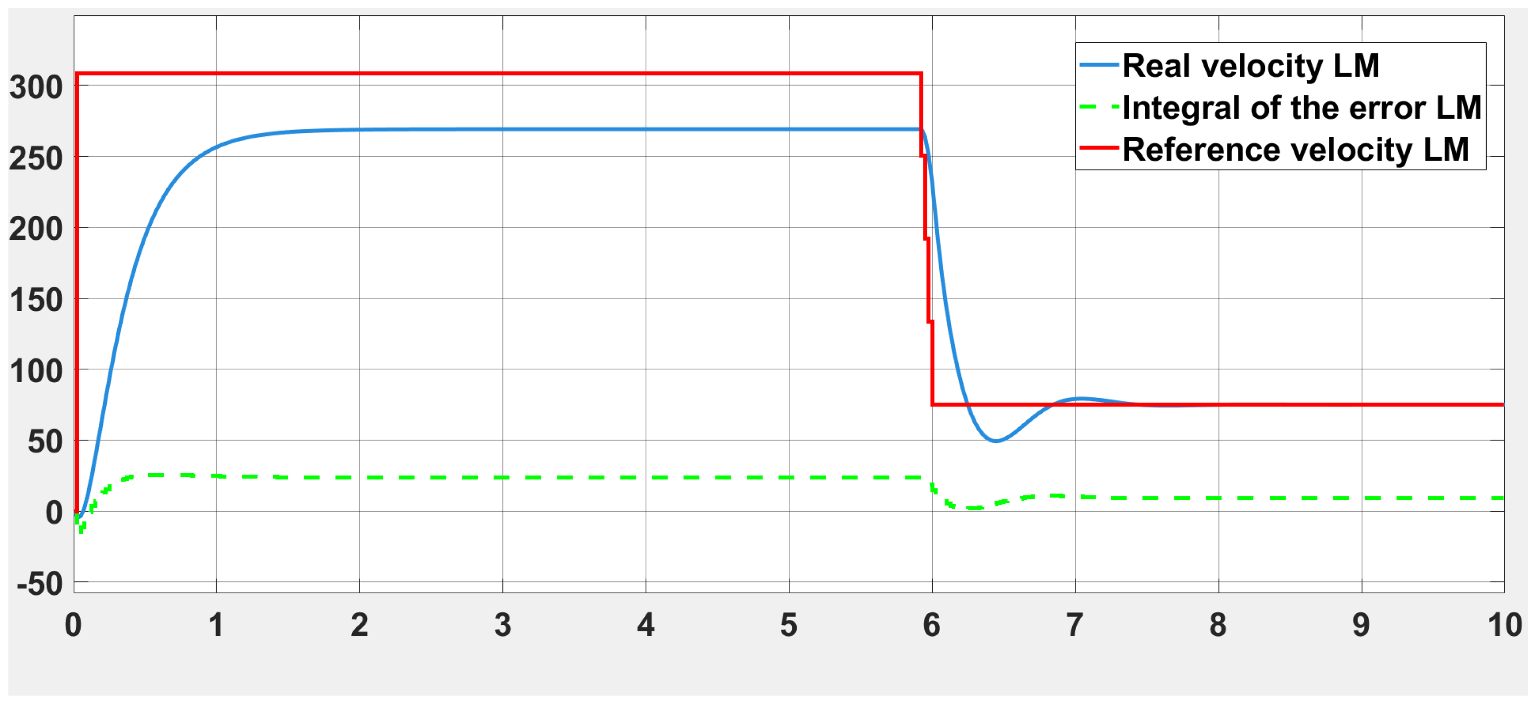
Figure 16.
Mathematical model of the robot implemented in Matlab/Simulink.
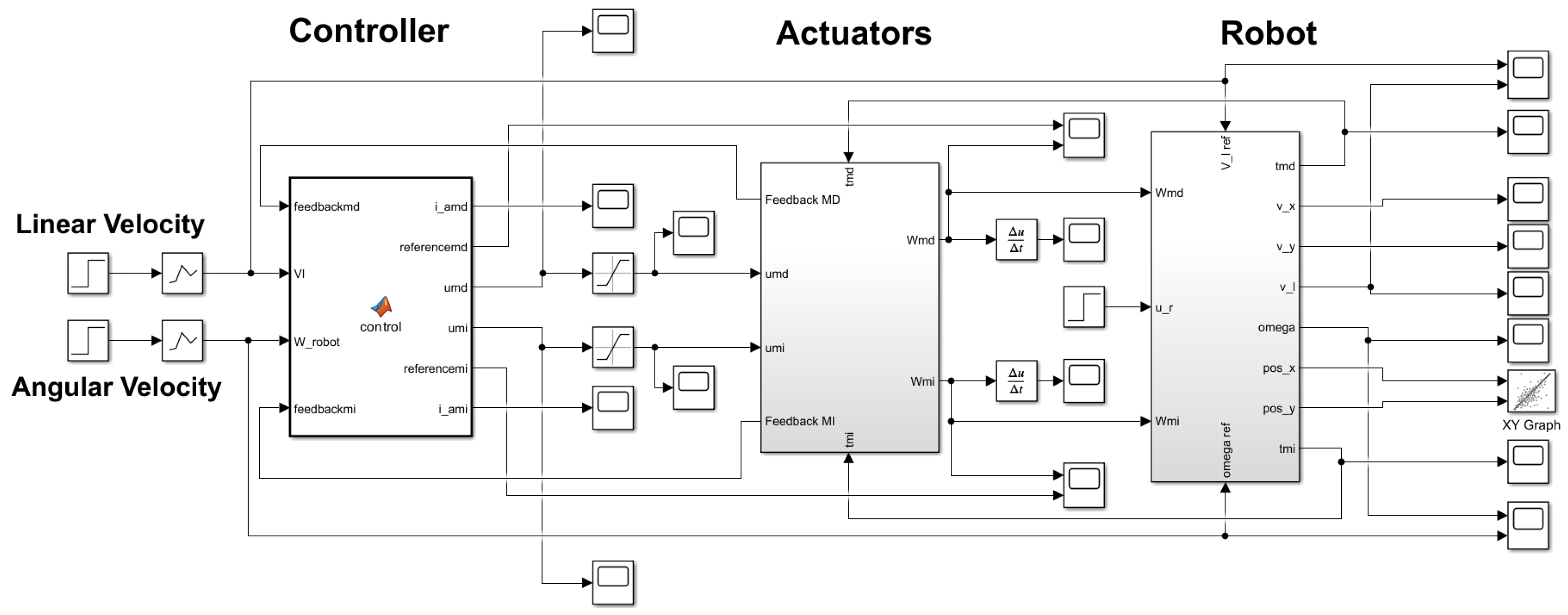
Figure 17.
Reference linear velocity and linear velocity achieved by the control system.
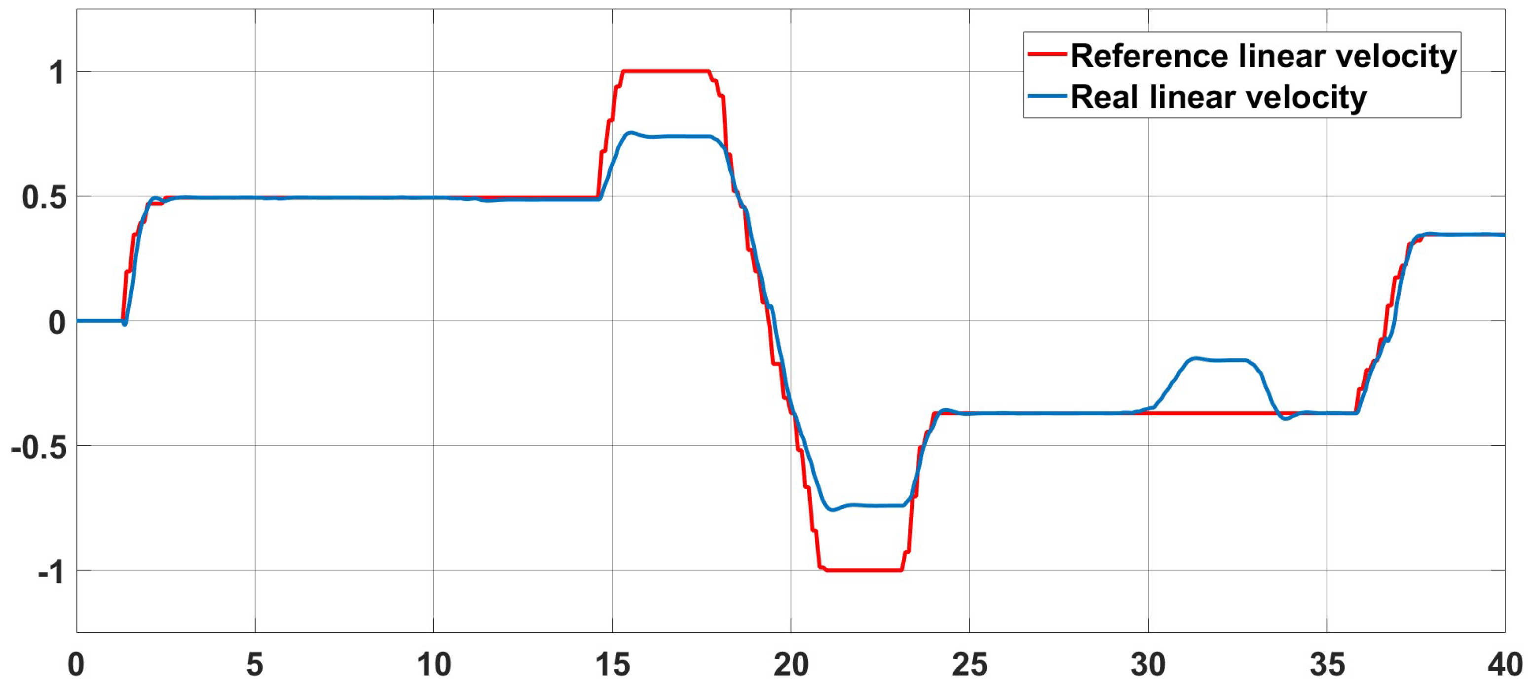
Figure 18.
Reference angular velocity and angular velocity achieved by the control system.
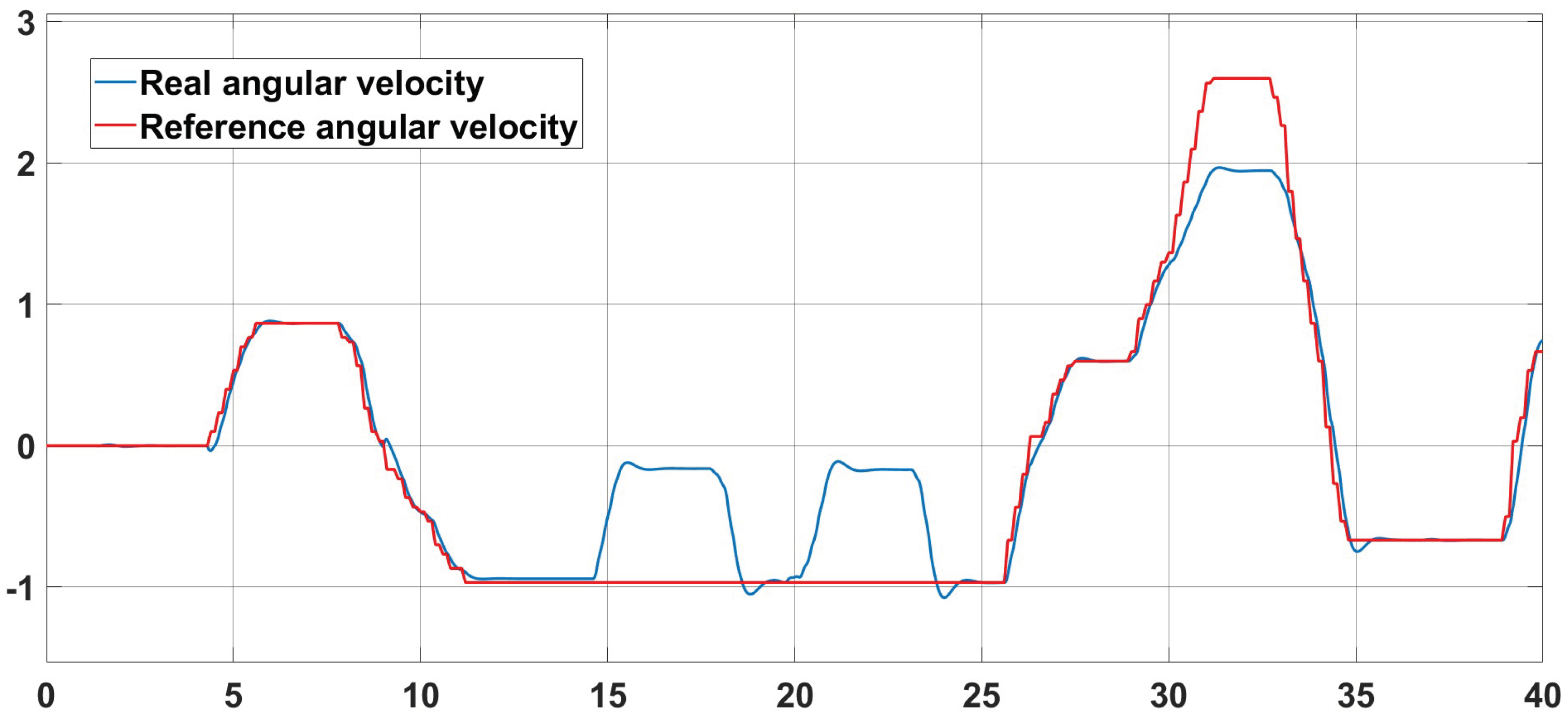
Figure 19.
Reference linear velocity and linear velocity achieved by the control system.
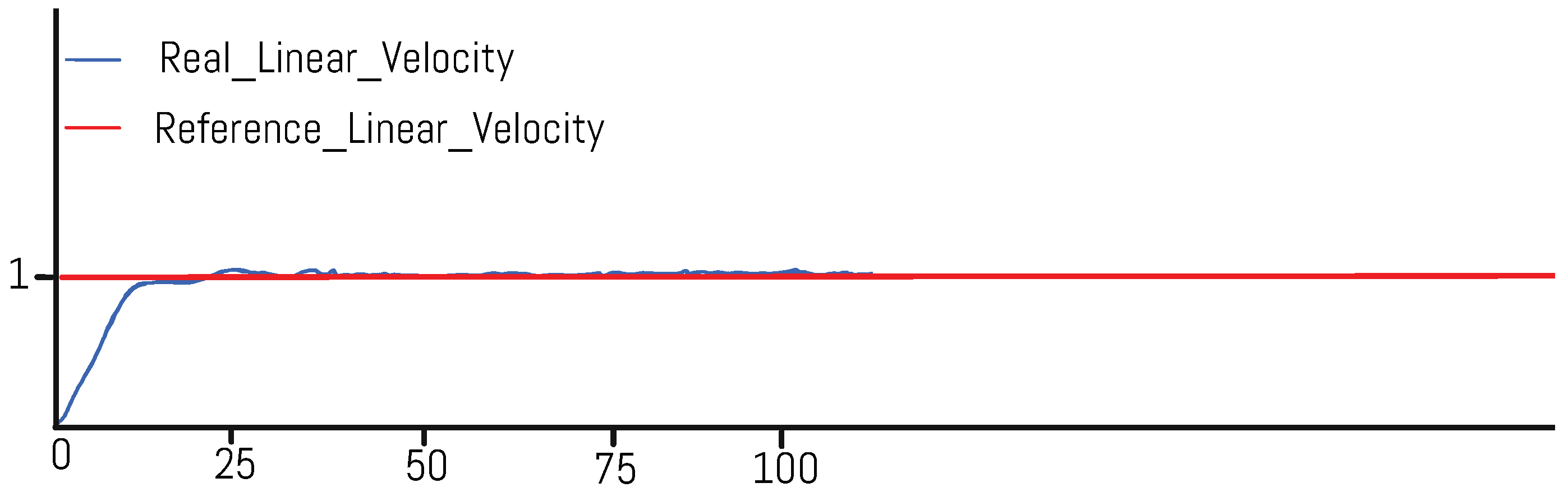
Figure 20.
Reference angular velocity and angular velocity achieved by the control system.
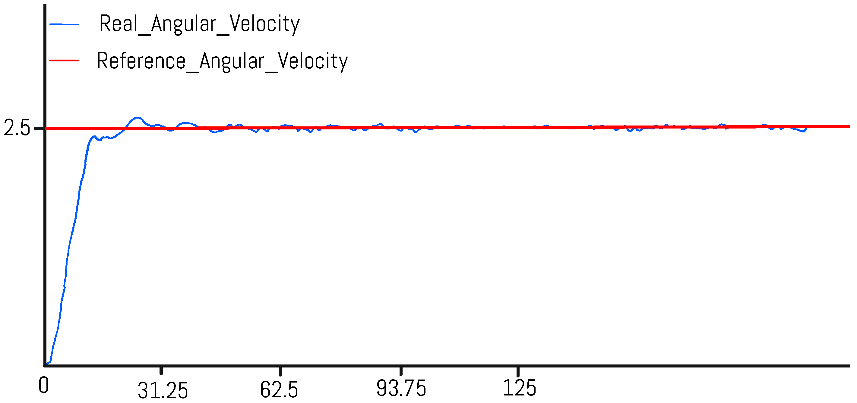
Figure 21.
Topic w_m with the most relevant data from the control system.
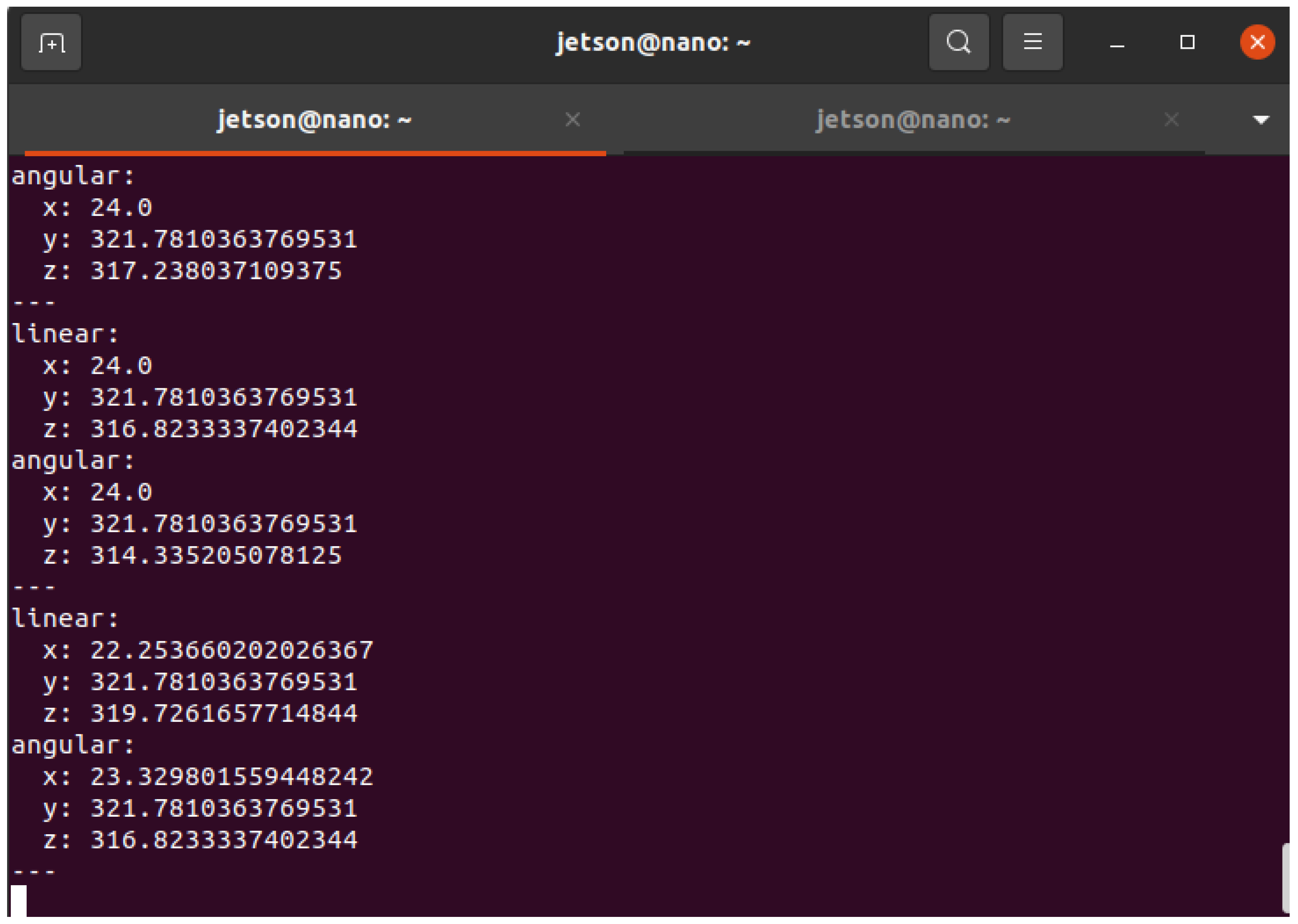

Table 1.
Known robot variables.
| Variable | Valor |
|---|---|
| Distance between wheels (L) | 0.650048 m |
| Track sprocket radius (r) | 0.07286 m |
| Number of motor output teeth (N1) | 18 |
| Number of teeth of the track sprocket (N2) | 27 |
| Mass of the structure | 6.949 kg |
| Track mass | 5.435 kg |
| Wheel mass | 3.589 kg |
| Front sprocket mass | 2.898 kg |
| Rear sprocket mass | 2.36 kg |
| Casing mass | 6.464 kg |
| Other components | 13.667 kg |
| Robot inertia () | 15.3 kg· m2 |
| Maximum angular velocity of motor () | 321.6 rad/s |
| Maximum motor torque () | 1.1333 Nm |
| Gearbox motor transmission ratio () | 1/15 |
| Motor supply voltage | 24 V |
Table 2.
Established parameters.
| Parameter | Value |
|---|---|
| Maximum linear speed of the robot (V) | 1.03396 m/s |
| Maximum angular velocity of the robot () | 3.18119 rad/s |
| Maximum angular acceleration of the motors () | 1000 rad/s2 |
Table 3.
Approximate parameters of the right motor.
| Parameter | Unit |
|---|---|
| KT | 0.1039 Nm/A |
| Kb | 0.0694 V· s/rad |
| Im | 0.000512 kg· m2 |
| b | 0.000251 Nm · s /rad |
| La | 0.153063 H |
| Ra | 2.2 |
Table 4.
Approximate parameters of the left motor.
| Parameter | Unit |
|---|---|
| KT | 0.1086 Nm/A |
| Kb | 0.0694 V· s/rad |
| Im | 0.000542 kg· m2 |
| b | 0.000272 Nm · s /rad |
| La | 0.164792 H |
| Ra | 2.3 |
Table 5.
PID controller parameters for the robot’s motors.
| Parameter | Right motor | Left motor |
| kp | 0.149347 | 0.158561 |
| 0.067278 | 0.069166 | |
| 0.150127 | 0.158682 |
Disclaimer/Publisher’s Note: The statements, opinions and data contained in all publications are solely those of the individual author(s) and contributor(s) and not of MDPI and/or the editor(s). MDPI and/or the editor(s) disclaim responsibility for any injury to people or property resulting from any ideas, methods, instructions or products referred to in the content. |
© 2025 by the authors. Licensee MDPI, Basel, Switzerland. This article is an open access article distributed under the terms and conditions of the Creative Commons Attribution (CC BY) license (http://creativecommons.org/licenses/by/4.0/).
Copyright: This open access article is published under a Creative Commons CC BY 4.0 license, which permit the free download, distribution, and reuse, provided that the author and preprint are cited in any reuse.


