Decentralized Adaptive Control of Closed-Kinematic Chain Mechanism Manipulators

1. Introduction

Robot manipulators, whose structure assumes a closed-kinematic chain mechanism (CKCM) have attracted great attention from robotic researchers due to their advantages over their counterpart, namely manipulators with open kinematic chain mechanism (OKCM) [1]. CKCM manipulators can mitigate weaknesses of OKCM manipulators such as low stiffness, poor stability, small payload and accumulated and amplified errors from link to link [2]. The CKCM was first employed in the design and construction of the Stewart Platform (SP) that possesses 6 degrees of freedom (DOF) [3]. Nowadays, the SP has a wide application area in spacecraft simulation, medical rehabilitation and high-speed assembly operation, vehicle dynamics, high-speed train dynamics, airplane dynamics, drone manipulation, medical rehabilitation and high-speed assembly operation [4,31,32].

In order for a robot to track a desired trajectory, a closed-loop feedback controller employs sensors to be aware of its surroundings and then adjusts appropriate control strategy to achieve a desired performance like the way a human brain works. In general, robotic systems are complicated, time-varying and highly nonlinear systems with uncertainties and disturbances in their working environment [5]. Moreover, due to the closed-loop structure of CKCM manipulators, the motion of each active joint is constrained by the motion of other active joints. Thus, the lack of synchronization between active joints will lead to a large coupling effect, which degrades the performance of the whole system or even damages its mechanical structure, especially at high speed and large payload. Therefore, it is essential for a CKCM manipulator to possess a synchronized controller that has the capacity to adapt and improve itself under changing conditions without human intervention and to force each active joint to follow its desired trajectory as close as possible while synchronizing its motion with the other active joint’s motions in a defined synchronous manner.

Recently, synchronization method based on the cross-coupling control technology has been developed to solve the above problem by allowing each control loop to receive feedback from itself as well as from the others to achieve better coordination and then improve the manipulator performance significantly [6]. This approach is a powerful tool for not only CKCM manipulators but also systems that require multiple objects to operate simultaneously to achieve a common goal such as swarm of mobile robot [7,8] or multiple robotic manipulator systems [9,10].

Most existing synchronized control schemes are model-based adaptive control schemes [11,12] and their implementation requires a precise dynamical model of the manipulator [13,14,15]. Due to the fact that it is difficult if not possible to acquire a precise dynamical model of the manipulator and its associated mathematical calculation is computationally intensive, these synchronized control schemes are not suitable for real-time applications of CKCM manipulators particularly of those with more than 2 DOFs. To tackle the above dynamic modelling issue, robotic researchers have considered intelligent approaches such as fuzzy logic [16,17] and artificial neural network control schemes [18,19]. However, these intelligent controllers exhibited shortcomings such as assurance of stability, high computational demand, slow convergence rate, and time-consuming training process. Finally, the authors in [20,21,22] considered synchronized control schemes that have simple structures and do not require the knowledge of the manipulator dynamics in the implementation of their control laws. However, their controller gains must still be selected based on conservative estimates of the manipulator dynamic model, which could be problematic and impractical.

During the trajectory tracking processes, CKCM manipulators can be treated as a group of multi OKCM manipulators holding the same payload. Hence, it is possible to develop a decentralized control scheme in which each active joint is controlled independently to minimize the computational cost and move synchronously to achieve the desired tracking performance of the moving platform [22].

In this paper, we develop a new decentralized adaptive synchronized control (DASC) scheme for CKCM manipulators. Unlike conventional decentralized control schemes [23], each sub-controller of the DASC scheme receives feedback from not only its active joint but also from 2 neighboring ones. Then, by applying the model reference adaptive control (MRAC) technique based on the Lyapunov direct method into the synchronized control method, the DASC scheme guarantees the global asymptotic convergence of tracking errors to zero, while synchronizing all active joint’s motion and overcoming uncertainties and disturbances. Moreover, the DASC scheme whose controller gains are updated by an adaptation law driven only by the actual and desired trajectories of active joints is computationally efficient and thus is suitable for real-time applications.

The structure of this paper is as follows. Section 2 describes the synchronization control method and Section 3 presents the development of the DASC scheme. Section 4 presents and discusses the results of a computer simulation study conducted to evaluate the effectiveness of the DASC scheme in comparison with another existing adaptive control scheme. Section 5 concludes the paper with summary and future research directions.

2. Synchronization Control

For a CKCM manipulator with $n$ active joints, the synchronization goal can be described by

$${\displaystyle \frac{q_1\left(t\right)}{q_{d1}\left(\mathrm{t}\right)}}={\displaystyle \frac{q_2\left(t\right)}{q_{d2}\left(\mathrm{t}\right)}}=\dots ={\displaystyle \frac{q_n\left(t\right)}{q_{dn}\left(\mathrm{t}\right)}}$$

(1)

where $q_{di}$ and $q_i\left(t\right)$denote the desired and actual trajectory of the $i^{th}$ active joint, respectively.

If all ratios in (1) are equal or in other words, if Equation (1) is valid, then all active joints will move in a synchronous manner [20]. However, considering synchronization of all active joints may lead to a heavy computational burden especially when the number of active joints is large.

We proceed to rewrite (1) as a set of subgoals

$${\displaystyle \frac{q_i\left(t\right)}{q_{di}\left(t\right)}}={\displaystyle \frac{q_{i+1}\left(t\right)}{q_{di+1}\left(t\right)}}$$

(2)

From subgoals (2), synchronization functions are defined as

$$\left\{\begin{array}{c}{f}_1\left[q_1\left(t\right),q_2\left(t\right)\right]={\displaystyle \frac{q_1\left(t\right)}{q_{d1}}}-{\displaystyle \frac{q_2\left(t\right)}{q_{d2}}}=0\\ f_2\left[q_2\left(t\right),q_3\left(t\right)\right]={\displaystyle \frac{q_2\left(t\right)}{q_{d2}\left(t\right)}}-{\displaystyle \frac{q_3\left(t\right)}{q_{d3}\left(t\right)}}=0\\ ⋮\\ f_i\left[q_i\left(t\right),q_{i+1}\left(t\right)\right]={\displaystyle \frac{q_i\left(t\right)}{q_{di}\left(t\right)}}-{\displaystyle \frac{q_{i+1}\left(t\right)}{q_{di+1}\left(t\right)}}=0\\ ⋮\\ f_n\left[q_n\left(t\right),q_1\left(t\right)\right]={\displaystyle \frac{q_n\left(t\right)}{q_{dn}\left(t\right)}}-{\displaystyle \frac{q_1\left(t\right)}{q_{d1}\left(t\right)}}=0\end{array}\right.$$

(3)

Using Taylor Series [30] to expand (3) at the desired joint trajectories $q_{di}(t$) to obtain

$$f_i\left[q_i\left(t\right),q_{i+1}\left(t\right)\right]=f_i\left[q_{di}\left(t\right),q_{di+1}\left(t\right)\right]+\sum _{j=i}^{j=i+1}\begin{array}{c}\left[\left.{\displaystyle \frac{\partial f_i\left(.\right)}{\partial q_j}}\right|\right]\\ { q}_{di}\left(t\right)\end{array}\left\{q_j\left(t\right)-q_{dj}\left(\mathrm{t}\right)+\mathcal{O}\left[q_j\left(t\right)\right]\right\}=-\sum _{j=i}^{j=i+1}\begin{array}{c}\left[\left.{\displaystyle \frac{\partial f_i\left(.\right)}{\partial q_j}}\right|\right]\\ q_{di}\left(t\right)\end{array}{q}_{ej}\left(t\right)+\mathcal{O}\left[q_j\left(t\right)\right]$$

(4)

where $\mathcal{O}\left[q_j\left(t\right)\right]$ denotes the higher order terms.

Considering only the first-order derivative, then (4) becomes

$$f_i\left[q_i\left(t\right),q_{i+1}\left(t\right)\right]={\displaystyle \frac{q_{ei}\left(t\right)}{q_{di}\left(t\right)}}-{\displaystyle \frac{q_{ei+1}\left(t\right)}{q_{di+1}\left(t\right)}}=0$$

(5)

where

$$q_{ei}\left(t\right)=q_{di}\left(t\right)-q_i\left(t\right)$$

(6)

and $q_{ei}\left(t\right),q_{di}\left(t\right),q_i\left(t\right)$ denote tracking error trajectory, desired trajectory and actual trajectory of the $ith$ active joint, respectively. Next, we define the synchronization errors as [20]

$$\begin{array}{c}{\epsilon }_1\left(t\right)=p_1\left(t\right)q_{\mathrm{e}1}\left(t\right)-p_2\left(t\right)q_{\mathrm{e}2}\left(t\right)\\ {\epsilon }_2\left(t\right)=p_2\left(t\right)q_{\mathrm{e}2}\left(t\right)-p_3\left(t\right)q_{\mathrm{e}3}\left(t\right)\\ ⋮\\ {\epsilon }_i\left(t\right)=p_i\left(t\right)q_{\mathrm{e}i}\left(t\right)-p_{i+1}\left(t\right)q_{\mathrm{e}i+1}\left(t\right)\\ ⋮\\ {\epsilon }_n\left(t\right)=p_n\left(t\right)q_{en}\left(t\right)-p_1\left(t\right)q_{\mathrm{e}1}\left(t\right)\end{array}$$

(7)

where ${\epsilon }_i$ represents the synchronization error of the $i^{th}$ active joint and $p_i\left(\mathrm{t}\right)={\displaystyle \frac{1}{q_{di}\left(t\right)}}$ and $c_i\left(t\right)$ is bounded. Obviously, if all synchronization errors in (7) are equal to zero, then the synchronization goal (1) is automatically achieved.

It is noted that by making all ${\epsilon }_i\left(t\right)=0$, only the synchronization goal is achieved. However, the goal of the control scheme is to drive both tracking and synchronization errors to zero.

Consequently, an error encompassing both synchronization and tracking should be defined. Thus, we define the cross-coupling errors that combine both tracking errors and synchronization errors as [29]

$$\begin{array}{c}{e_1}^{\mathrm{*}}\left(\mathrm{t}\right)=q_{\mathrm{e}1}\left(\mathrm{t}\right)+\beta {\int }_0^t{[\epsilon }_1\left(w\right)-{\epsilon }_n\left(w\right)]dw\\ {e_2}^{\mathrm{*}}\left(\mathrm{t}\right)=q_{\mathrm{e}2}\left(\mathrm{t}\right)+\beta {\int }_0^t{[\epsilon }_2\left(w\right)-{\epsilon }_1\left(w\right)]dw\\ ⋮\\ {e_i}^{\mathrm{*}}\left(\mathrm{t}\right)=q_{\mathrm{e}i}\left(\mathrm{t}\right)+\beta {\int }_0^t\left[{\epsilon }_i\left(w\right)-{\epsilon }_{i-1}\left(w\right)\right]dw\\ ⋮\\ {e_n}^{\mathrm{*}}\left(\mathrm{t}\right)=q_{en}\left(\mathrm{t}\right)+\beta {\int }_0^t{[\epsilon }_n\left(w\right)-{\epsilon }_{n-1}\left(w\right)]dw\end{array}$$

(8)

where $\beta$ is a positive coupling parameter and ${e_i}^{\mathrm{*}}\left(\mathrm{t}\right)$ represents the cross-coupling error of the $i^{th}$ active joint. From (7) and (8), it is noted that the local controller of each joint receives feedback information from not only itself but also the two neighboring ones.

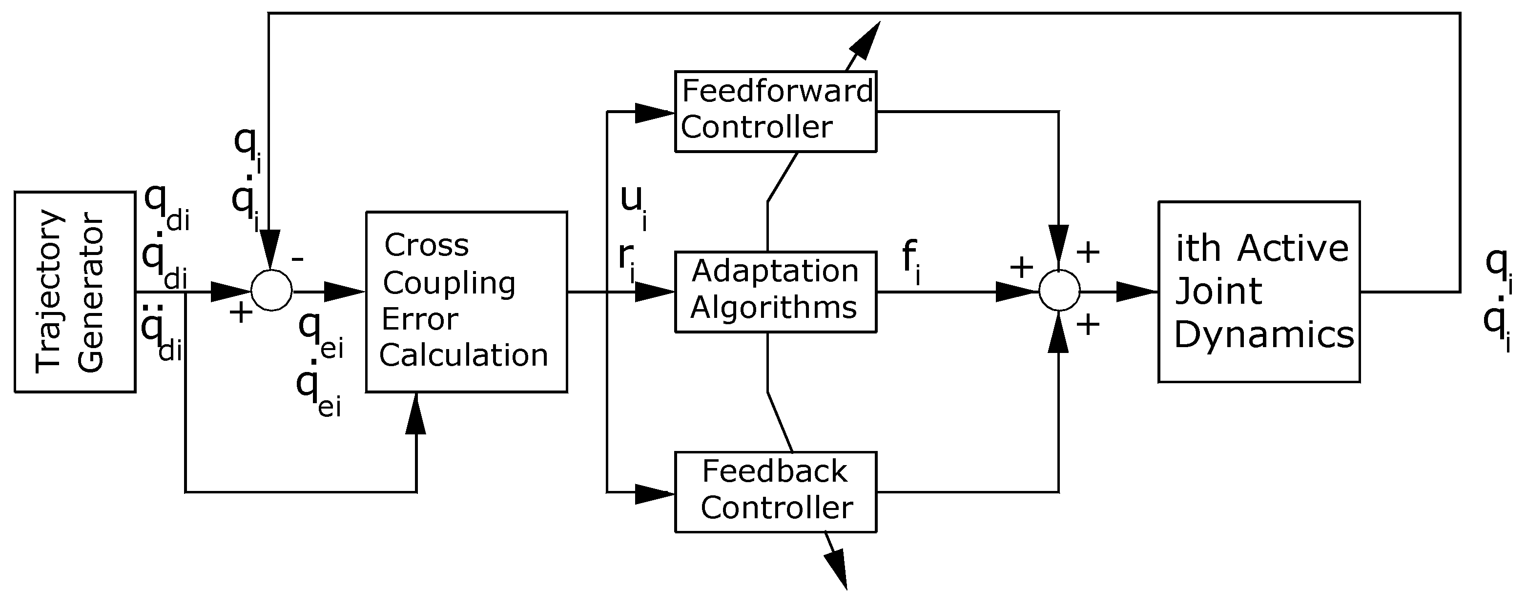
3. Development of the DASC Scheme

The dynamics of a robot manipulator having n active joints can be expressed in joint-space as [25]

$$M\left(q\right)\ddot{q}+N\left(q,\dot{q}\right)+G\left(q\right)+H\left(\dot{q}\right)=T\left(t\right)$$

(9)

where $q$ is the nx1 vector of joint displacement, $M\left(q\right)$ is the n x n symmetric positive definite inertia matrix, $N\left(q,\dot{q}\right)$ is the n x 1 Coriolis and centrifugal torque vector, $G\left(q\right)$ is the n x 1 gravitational torque vector and $H\left(\dot{q}\right)$ is the n x 1 frictional torque vector.

The $ith$ subsystem of the dynamical system (9) can be written as the following decentralized form [23]

$$m_{ii}\left(q\right){\ddot{q}}_{ii}\left(t\right)+\left[{\sum }_{\begin{array}{c}j=1\\ j\ne 1\end{array}}^6{m}_{ij}\left(q\right){\ddot{q}}_j\left(t\right)\right]+n_i\left(q,\dot{q}\right)+g_i\left(q\right)+h_i\left(\dot{q}\right)=T_i\left(t\right)$$

(10)

where $T_i$ is the control input of the $ith$ active joint.

As seen in (10),the $ith$ subsystem not only contains the gravity, friction, Coriolis and centrifugal torque, namely $n_i\left(q,\dot{q}\right)+g_i\left(q\right)+h_i\left(q\right)$ for the $ith$ active joint but also is coupled between it and the remaining subsystems shown by the term $\left[\sum _{\begin{array}{c}j=1\\ j\ne 1\end{array}}^6{m}_{ij}\left(q\right){\ddot{q}}_j\left(t\right)\right].$

Let

$$d_i\left(q,\dot{q},\ddot{q}\right)={\sum }_{\begin{array}{c}j=1\\ j\ne 1\end{array}}^6{m}_{ij}\left(q\right){\ddot{q}}_j\left(t\right)+n_i\left(q,\dot{q}\right)+g_i\left(q\right)+h_i\left(\dot{q}\right)$$

(11)

Then (10) becomes

$$m_{ii}\left(q\right){\ddot{q}}_{ii}\left(t\right)+d_i\left(q,\dot{q},\ddot{q}\right)=T_i\left(t\right)$$

(12)

Next, we define a command vector ui(t) as

$$u_i\left(t\right)=q_{di}\left(t\right)+\beta {\int }_0^t{[\epsilon }_n\left(w\right)-{\epsilon }_{n-1}\left(w\right)]dw+\alpha {\int }_0^t{e_i}^{\mathrm{*}}\left(w\right)dw$$

(13)

where $q_{di}\left(t\right)$ denotes the desired trajectory of the $i^{th}$ active joint and $\alpha$ is a positive constant. We also define a generalized error ri(t) as

$$r_i\left(t\right)=u_i\left(t\right)-q_i\left(t\right)={e_i}^{\mathrm{*}}\left(t\right)+\alpha {\int }_0^t{e_i}^{\mathrm{*}}\left(w\right)dw$$

(14)

Now a control law for the $ith$ subsystem in (10), can be defined as

$$T_i\left(t\right)=f_i\left(t\right)+\left[k_{0i}\left(t\right)r_i\left(t\right)+k_{1i}\left(t\right){\dot{r}}_i\left(t\right)\right]+\left[a_i\left(t\right)u_i\left(t\right)+b_i\left(t\right){\dot{u}}_i\left(t\right)+c_i\left(t\right){\ddot{u}}_i\left(t\right)\right]$$

(15)

Substituting (15) into (10) in light of (12) and dropping the subscript i for simplicity, we obtain the error differential equation in terms of the generalized error r(t) which is indeed r_i(t) as

$$m\ddot{r}\left(t\right)+k_1\left(t\right)\dot{r}\left(t\right)+k_0\left(t\right)r\left(t\right)=d-f\left(t\right)-a\left(t\right)u\left(t\right)-b\left(t\right)\dot{u}\left(t\right)+\left(m-c\right)\ddot{u}\left(t\right)$$

(16)

Let us define the 2x1 position-velocity error vector $X\left(t\right)=\left(\begin{array}{c}r\left(t\right)\\ \dot{r}\left(t\right)\end{array}\right)$ and then express Equation (16) in a state space form as

$$\dot{X}\left(t\right)=\left(\begin{array}{cc}0& 1\\ {-∆}_1& -{∆}_2\end{array}\right)X\left(t\right)+\left(\begin{array}{c}0\\ {∆}_0\end{array}\right)+\left(\begin{array}{c}0\\ {∆}_3\end{array}\right)u\left(t\right)+\left(\begin{array}{c}0\\ {∆}_4\end{array}\right)\dot{u}\left(t\right)+\left(\begin{array}{c}0\\ {∆}_5\end{array}\right)\ddot{u}\left(t\right)$$

(17)

where the variables ${∆}_1={\displaystyle \frac{k_0}{m}}$; ${∆}_2={\displaystyle \frac{k_1}{m}}$; ${∆}_0={\displaystyle \frac{d-f}{m}}$; ${∆}_3={\displaystyle \frac{-a}{m}};$ ${∆}_4={\displaystyle \frac{-b}{m}}$; ${∆}_5={\displaystyle \frac{\left(m-c\right)}{m}}$ contain the adjustable controller gains $k_1\left(t\right),k_0\left(t\right),f\left(t\right),a\left(t\right),b\left(t\right),\mathrm{a}\mathrm{n}\mathrm{d}c\left(t\right).$

Equation (17) represents the “adjustable system” in the framework of MRAC. Next, the desired performance of the $i^{th}$ active joint can be specified in terms of a second-order homogeneous differential equation

$${\ddot{r}}_m\left(t\right)+2\omega \xi {\dot{r}}_m\left(t\right)+{\omega }^2{r}_m\left(t\right)=0$$

(18)

where $\xi$ is the damping ratio, $\omega$is the natural frequency and $r_m\left(t\right)$ represents the desired trajectory of $r\left(t\right).$

Equation (18) can be written in a state space form as

$${\dot{X}}_m\left(t\right)=\left(\begin{array}{cc}0& 1\\ {-D}_1& -D_2\end{array}\right)X_m\left(t\right)=D{X}_m\left(t\right)$$

(19)

where $D=\left(\begin{array}{cc}0& 1\\ {-D}_1& -D_2\end{array}\right)$, $X_m\left(t\right)=\left(\begin{array}{c}{r}_m\left(t\right)\\ {\dot{r}}_m\left(t\right)\end{array}\right)$, $D_1={\omega }^2$, $D_2=2\omega \xi$ and $r_m\left(t\right)$ and ${\dot{r}}_m\left(t\right)$ are the desired generalized position error and velocity errors, respectively.

Equation (19) represents the “reference model” and its solution is found as

$$X_m\left(t\right)=\exp \left(Dt\right)X_m\left(0\right)$$

(20)

which under the assumption that the initial values of the actual and the desired trajectory are identical. In other words, $X_m\left(0\right)=0$ yields $X\left(0\right)=0$.

We define the adaptation error vector E(t) as

$$E\left(t\right)=X_m\left(t\right)-X\left(t\right)$$

(21)

Then from (17) and (19), we obtain

$$\dot{E}\left(t\right)=\left(\begin{array}{cc}0& 1\\ {-D}_1& -D_2\end{array}\right)E\left(t\right)+\left(\begin{array}{cc}0& 1\\ {∆}_1{-D}_1& {∆}_1{-D}_1\end{array}\right)X\left(t\right)+\left(\begin{array}{c}0\\ {-∆}_0\end{array}\right)+\left(\begin{array}{c}0\\ {-∆}_3\end{array}\right)u\left(t\right)+\left(\begin{array}{c}0\\ -{∆}_4\end{array}\right)\dot{u}\left(t\right)+\left(\begin{array}{c}0\\ -{∆}_5\end{array}\right)\ddot{u}\left(\mathrm{t}\right)$$

(22)

Now, the controller adaptation laws will be derived to achieve the control objective, expressed by $X\left(t\right)⟶X_m\left(t\right)$ or $E\left(t\right)⟶$0 as t$\to$ $\mathrm{\infty }$. To achieve this, we select a Lyapunov function candidate $v\left(t\right)$ [23] such that

$$v\left(t\right)=E^{T}PE+Q_o{\left({\mathsf{\Delta }}_0-{{\mathsf{\Delta }}_0}^{\mathrm{*}}\right)}^2+Q_1{\left({\mathsf{\Delta }}_1{-D}_1-{{\mathsf{\Delta }}_1}^{\mathrm{*}}\right)}^2+Q_2{\left({\mathsf{\Delta }}_2{-D}_2-{{\mathsf{\Delta }}_2}^{\mathrm{*}}\right)}^2+Q_3{\left({\mathsf{\Delta }}_3-{{\mathsf{\Delta }}_3}^{\mathrm{*}}\right)}^2+Q_4{\left({\mathsf{\Delta }}_4-{{\mathsf{\Delta }}_4}^{\mathrm{*}}\right)}^2+Q_5{\left({\mathsf{\Delta }}_5-{{\mathsf{\Delta }}_5}^{\mathrm{*}}\right)}^2$$

(23)

where ${{\mathsf{\Delta }}_0}^{\mathrm{*}},{{\mathsf{\Delta }}_1}^{\mathrm{*}},\dots ,{{\mathsf{\Delta }}_6}^{\mathrm{*}}$ are function of time and $Q_o,Q_1,\dots ,Q_5$ are arbitrary positive scalar.

To stabilize the linear part of (22), it is sufficient to choose ${\xi }_i$ and ${\omega }_i$ such that the matrix D becomes Hurwitz, or all eigenvalues of D have negative real parts. If so, there exists a symmetric positive definite matrix P=$\left[\begin{array}{cc}{P}_1& P_2\\ P_2& P_3\end{array}\right]$ to satisfy the following Lyapunov Equation

$$PD+D^{T}P=-Q$$

(24)

for any arbitrary symmetric positive definite matrix Q.

Finally, from [23], particularly in the section entitled Derivation of the Adaption Laws, the derivative of $v\left(t\right)$, namely $\dot{v}\left(t\right)$ will be negative definite of $E\left(t\right)$ when we choose the following adaptation laws

$$f\left(t\right)=f\left(0\right)+{\eta }_2\mathsf{\Omega }\left(\mathrm{t}\right)+{\eta }_1{\int }_0^t\mathsf{\Omega }\left(\mathrm{w}\right)\mathrm{d}\mathrm{w}$$

$$k_0\left(t\right)=k_0\left(0\right)+{\gamma }_2\mathsf{\Omega }\left(\mathrm{t}\right)\mathrm{r}\left(t\right)+{\gamma }_1{\int }_0^t\mathsf{\Omega }\left(\mathrm{w}\right)\mathrm{r}\left(\mathrm{w}\right)\mathrm{d}\mathrm{w}$$

$$k_1\left(t\right)=k_1\left(0\right)+{\lambda }_2\mathsf{\Omega }\left(\mathrm{t}\right)\dot{r}\left(t\right)+{\lambda }_1{\int }_0^t\mathsf{\Omega }\left(\mathrm{w}\right)\dot{r}\left(\mathrm{w}\right)\mathrm{d}\mathrm{w}$$

$$a\left(t\right)=\mathrm{a}\left(0\right)+{\mu }_2\mathsf{\Omega }\left(\mathrm{t}\right)\mathrm{u}\left(\mathrm{t}\right)+{\mu }_1{\int }_0^t\mathsf{\Omega }\left(\mathrm{w}\right)\mathrm{u}\left(\mathrm{w}\right)\mathrm{d}\mathrm{w}$$

$$b\left(t\right)=b\left(0\right)+{\rho }_2\mathsf{\Omega }\left(\mathrm{t}\right)\dot{u}\left(t\right)+{\rho }_1{\int }_0^t\mathsf{\Omega }\left(\mathrm{w}\right)\dot{u}\left(w\right)\mathrm{d}\mathrm{w}$$

$$c\left(t\right)=c\left(0\right)+{\sigma }_2\mathsf{\Omega }\left(\mathrm{t}\right)\ddot{u}\left(t\right)+{\sigma }_1{\int }_0^t\mathsf{\Omega }\left(\mathrm{w}\right)\ddot{u}\left(\mathrm{w}\right)\mathrm{d}\mathrm{w}$$

where ${\eta }_1,{\gamma }_1,{\lambda }_1,{\mu }_1,{\rho }_1,{\sigma }_1$ are positive constant and ${\eta }_2,{\gamma }_2,{\lambda }_2,{\mu }_2,{\rho }_2,{\sigma }_2$ are zero or positive constant, $\mathsf{\Omega }\left(t\right)=P_{2}r\left(t\right)+P_3\dot{r}\left(t\right)$ where $P_2$ and $P_3$ are positive constant, depending on the reference model. Furthermore, $f$ (0), $k_0$ (0), $k_1$ (0), $a$ (0), $b\left(0\right)$,$c\left(0\right)$ which are the initial conditions of $f\left(t\right)$, $k_0\left(t\right)$, $k_1\left(t\right)$, $a\left(t\right)$, $b\left(t\right)$,$c\left(t\right)$, respectively, can be set arbitrarily.

As a result, $X\left(t\right)⟶$0 as $t\to$ $\mathrm{\infty }$ results in $\left[\begin{array}{c}{e_i}^{\mathrm{*}}\left(t\right)+\beta {\int }_0^t{e_i}^{\mathrm{*}}\left(w\right)dw\\ {{\dot{e}}_i}^{\mathrm{*}}\left(t\right)+\beta {e_i}^{\mathrm{*}}\left(t\right)\end{array}\right]⟶0$ as t$\to$ $\mathrm{\infty }$.

Then, ${e_i}^{\mathrm{*}}\left(t\right)⟶0$ and ${{\dot{e}}_i}^{\mathrm{*}}\left(t\right)⟶0$ as t$\to$ $\mathrm{\infty }$ [27]. Thus, ${q_{ei}\left(t\right)}_{,}$ ${\dot{q}}_{ei}\left(t\right)$ are bounded from (9) and from differentiating (9). Moreover, ${\dot{\epsilon }}_i\left(t\right)$ are bounded from differentiating (8), then ${\epsilon }_i\left(t\right)$ are uniformly continuous since every function which is differentiable and has bounded derivative is uniformly continuous [24].

From Barbalat’s Lemma [26], suppose that $f:\left[0,\mathrm{\infty }\right]\to \mathbb{R}$ is uniformly continuous and its derivative is bounded. Then, $f\left(t\right)⟶0$ as t$\to$ $\mathrm{\infty }$ holds. Therefore, ${\epsilon }_i\left(t\right)⟶0$ as t$\to$ $\mathrm{\infty }$ since ${\epsilon }_i\left(t\right)$ are uniformly continuous and ${\dot{\epsilon }}_i\left(t\right)$ are bounded. From (8) and (9), ${\epsilon }_i\left(t\right)⟶0$ and ${e_i}^{\mathrm{*}}\left(t\right)⟶0$ results in $e_i\left(t\right)⟶0$ as t$\to$ $\mathrm{\infty }$ for all $i=1-n$. Therefore, the control objective is achieved.

It is noted that the adaptation laws are solutions for controller gain matrices of control law (15) and based on the actual, desired performances and their derivatives. Furthermore, we note that the control law (15) consists of three terms

• The first term $f_i\left(t\right)$ represents auxiliary signal to improve the tracking performance and partly compensate for disturbance $d\left(t\right)$
• The second term ${\tau }_i^{fb}\left(t\right)=\left[k_{0i}\left(t\right)r_i\left(t\right)+k_{1i}\left(t\right){\dot{r}}_i\left(t\right)\right]$=${[k}_{0i}\left(t\right)+\alpha ]{e_i}^{\mathrm{*}}\left(t\right)+{\alpha k}_{0i}\left(t\right){\int }_0^t{e_i}^{\mathrm{*}}\left(w\right)dw]+k_{1i}\left(t\right)\dot{{e_i}^{\mathrm{*}}}\left(t\right)$ represents the PID feedback controller
• The last term ${\tau }_i^{ff}\left(t\right)=\left[a_i\left(t\right)u_i\left(t\right)+b_i\left(t\right){\dot{u}}_i\left(t\right)+c_i{\ddot{u}}_i\left(t\right)\right]$ represent the feedforward controller

The structure of the controller is shown in Figure 1. The required inputs of $ith$ controller is the desired position, velocity, acceleration of its active joint. The required measurements are the actual positions and velocities of its active joint and 2 adjacent ones.

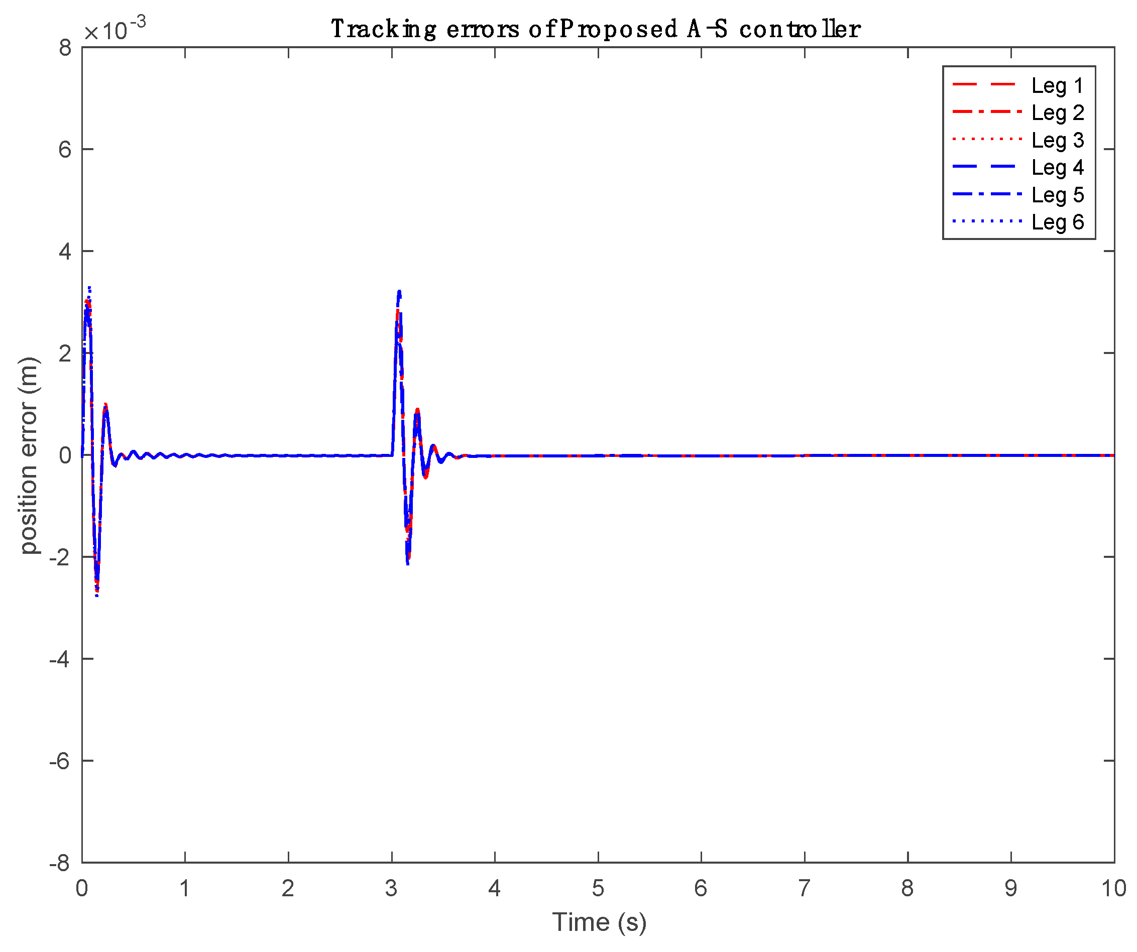
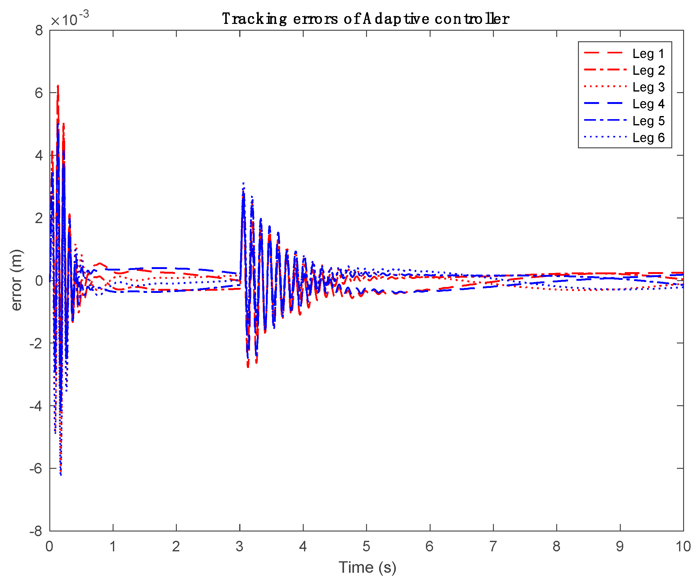
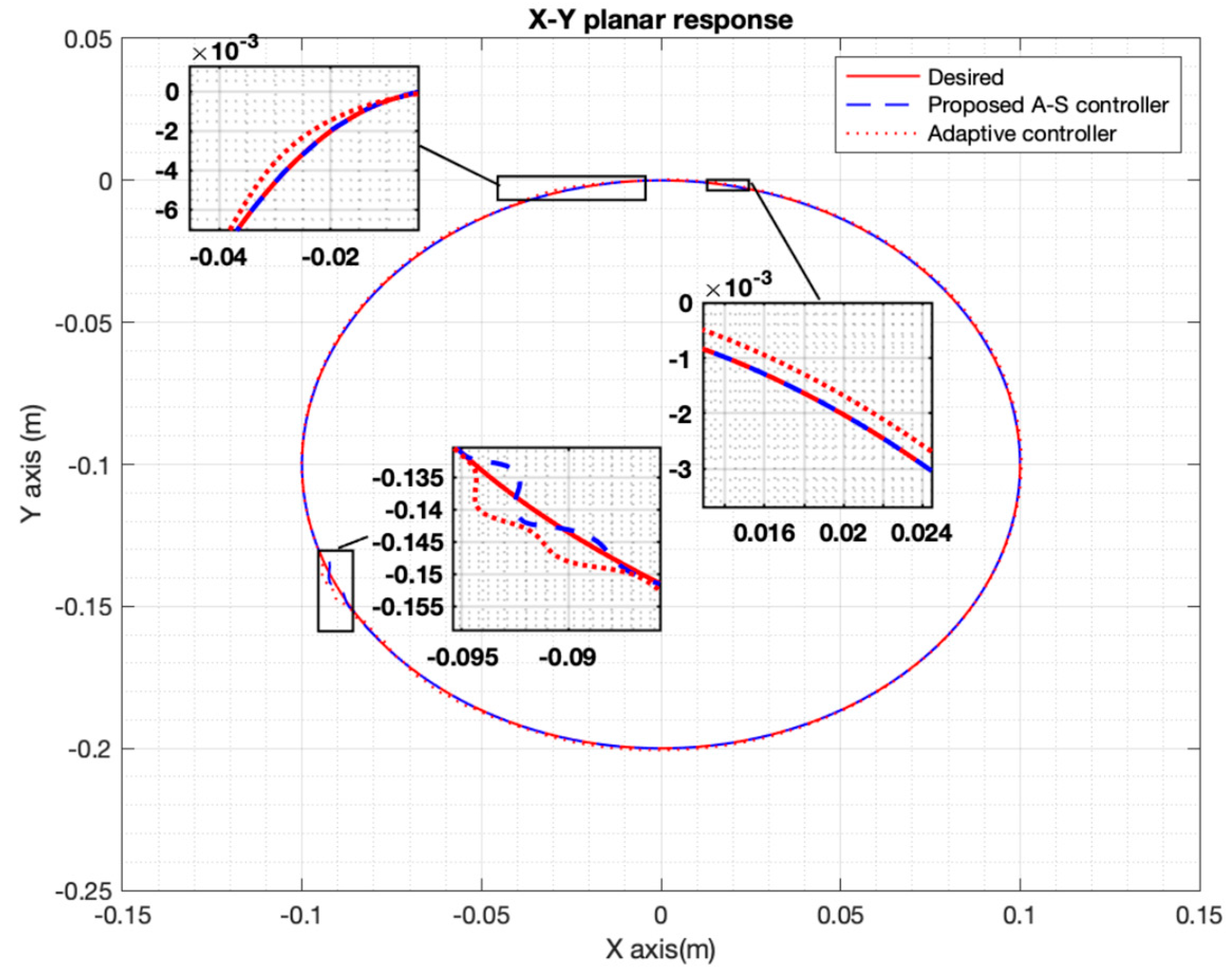
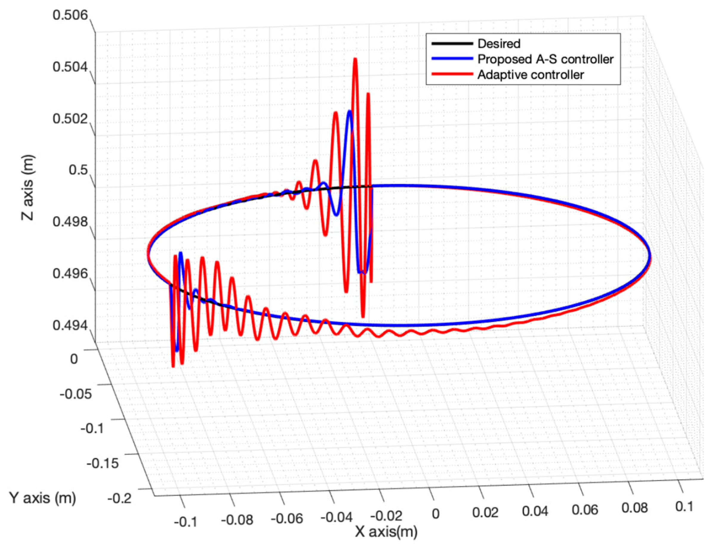
4. Computer Simulation Study

This section presents and discusses results of a computer simulation study conducted to evaluate the effectiveness of the developed DASC scheme applied to control the motion of a 6- DOF CKCM manipulator with properties listed in Table 1. The computer simulation study is carried out using MATLAB/Simulink. Figure 2 shows the Simulink model of the manipulator.

For comparison purpose, the developed DASC and the traditional adaptive controller developed by Seraji in [23] are employed track a reference model with the desired damping ratios and natural frequencies chosen as ωi = 10rad/s; ζi = 1, for i = 1, 2, 3,…, 6. We aim at comparing the performance of the DASC with the Seraji Controller when tracking a circular path in the X-Y plane, described by the following equations

$$\left\{\begin{array}{c}x\left(t\right)=0.1\cos \left(2\pi t\right) \left(m\right)\\ y\left(t\right)=0.1\sin \left(2\pi t\right) \left(m\right) \\ z\left(t\right)=0.5 \left(m\right) \end{array}\right.$$

$$\alpha \left(t\right)=\beta \left(t\right)=\gamma \left(t\right)=0\left(rad\right)$$

where $\alpha \left(t\right),\beta \left(t\right),\gamma \left(t\right)$ are rotations about the $x\left(t\right),y\left(t\right),z\left(t\right)$ axes. To evaluate the adaptive ability of the above controllers, a 40kg payload is suddenly applied at the center of the mass of the moving platform at time t=3 sec.

Figure 3 and Figure 4 show synchronization errors of the 2 controllers. From these figures, the DASC scheme can guarantee the global asymptotic convergence to zero of synchronization errors while the Seraji Controller cannot.

Figure 5 and Figure 6 show the tracking errors of 2 controllers. As seen from these figures, before a payload is applied, the Seraji Controller needs more time to force the manipulator approach to the steady state. When the payload is applied at 3s, the system with the DASC scheme enters the steady state after $t\ge 3.5s$ while the Seraji Controller cannot. Moreover, the steady-state errors of the DASC scheme are much smaller than those of the Seraji Controller.

Figure 7 and Figure 8 illustrate the trajectory tracking of 2 controllers in the X-Y and the X-Y-Z planes, respectively. As shown by these figures, the Seraji Controller gets off track at the beginning and after the introduction of the full payload. Moreover, the DASC scheme has a better adaptation to track the motion with a much smaller deviation from the desired trajectory until the end of the motion.

Table 2 shows that the average absolute position errors and the tracking and synchronization errors of the 6 legs of the manipulator of the DASC are significantly smaller than those of the Seraji Controller.

5. Conclusion

In this paper, by treating the trajectory tracking control of a CKCM manipulator as synchronized control of multi OKCM manipulators, we developed a new decentralized adaptive synchronized controller, called DASC for CKCM manipulators. The developed controller does not require any knowledge of the manipulator dynamics and guarantees the global asymptotic convergence of both tracking and synchronization errors while overcoming uncertainties and sudden changes in payload. Computer simulations conducted to study the performance of the DASC Controller in comparison with the Seraji Controller show that the DASC has better tracking performance. From our computer simulation study, we conclude that in general, adaptive controllers with synchronized error control perform better than those without it. Further work is to apply the DASC in controlling motion of real CKCM manipulators and compare its performance to that of existing adaptive controllers.

References

1. Merlet, J. P. Parallel robots (Vol. 128). Springer Science & Business Media. 2006.
2. Tsai, L. W. Robot analysis: the mechanics of serial and parallel manipulators. 1999, John Wiley & Sons.
3. Stewart, D., A Platform with Six Degrees of Freedom, Proc. Institute of Mechanical Engineering, vol. 180, part 1, No. 5, pp. 371-386, 1965-1966.
4. Dasgupta, B.; Mruthyunjaya, T. S. The Stewart platform manipulator: a review. Mechanism and machine theory. 2000, 35, 15–40. [Google Scholar]
5. Kelly, R.; Davila, V. S.; Perez, J. A. L. Control of robot manipulators in joint space. Springer Science & Business Media. 2006.
6. Y. Koren, “Cross-coupled biaxial computer control for manufacturing systems”, Journal of Dynamic Systems Measurement and Control, 1980.
7. Li, Y.; Nielsen, C. Position synchronized path following for a mobile robot and manipulator. 52nd IEEE Conference on Decision and Control, 2013, pp. 3541-3546.
8. Do, K. D. Synchronization motion tracking control of multiple underactuated ships with collision avoidance. IEEE Transactions on Industrial Electronics. 2016, 63, 2976–2989. [Google Scholar]
9. Bouteraa, Y.; Ghommam, J.; Poisson, G.; Derbel, N. Distributed synchronization control to trajectory tracking of multiple robot manipulators. Journal of Robotics. 2011. [Google Scholar]
10. Wang, C.; Sun, D. A synchronization control strategy for multiple robot systems using shape regulation technology. 2008 7th World Congress on Intelligent Control and Automation. 2008, pp. 467-472.
11. Shang, W.; Cong, S.; Ge, Y. Coordination motion control in the task space for parallel manipulators with actuation redundancy. IEEE Transactions on Automation Science and Engineering. 2012, 10, 665–673. [Google Scholar]
12. Sun, D.; Wang, C.; Shang, W.; Feng, G. A synchronization approach to trajectory tracking of multiple mobile robots while maintaining time-varying formations. IEEE Transactions on Robotics 2009, 25, 1074–1086. [Google Scholar]
13. Sun, D.; Mills, J. K. Adaptive synchronized control for coordination of two robot manipulators. In Proceedings 2002 IEEE International Conference on Robotics and Automation. 2002, (Cat. No. 02CH37292) (Vol. 1, pp. 976-981).
14. Zhu, W. H. On adaptive synchronization control of coordinated multi robots with flexible/rigid constraints. IEEE Transactions on Robotics. 2005, 21, 520–52. [Google Scholar]
15. Wang, H. Task-space synchronization of networked robotic systems with uncertain kinematics and dynamics. IEEE Transactions on Automatic Control. 2013, 58, 3169–3174. [Google Scholar]
16. Long, Y.; Yang, X. J. Robust adaptive fuzzy sliding mode synchronous control for a planar redundantly actuated parallel manipulator. 2012 IEEE International Conference on Robotics and Biomimetics (ROBIO) 2012, pp. 2264-2269.
17. Fuh, C. C.; Tsai, H. H.; Huang, C. C. A fuzzy cross-coupled linear quadratic regulator for improving the contour accuracy of bi-axis machine tools. In Proceedings of the 48h IEEE Conference on Decision and Control (CDC) held jointly with 2009 28th Chinese Control Conference 2009, pp. 4156-4161.
18. Zhao, D.; Zhu, Q.; Li, N.; Li, S. Neural networked based synchronized control for multiple robotic manipulators. 10th IEEE International Conference on Control and Automation (ICCA) 2013, pp. 1950-1955.
19. Le, D. K.; Ahn, K. K. Synchronization algorithm for controlling 3-R planar parallel pneumatic artificial muscle robot. 2011 11th International Conference on Control, Automation and Systems 2011, pp. 1588-1593.
20. Su, Y. X.; Sun, D.; Ren, L.; Wang, X.; Mills, J. K. Nonlinear PD synchronized control for parallel manipulators. In Proceedings of the 2005 IEEE international conference on robotics and automation 2005, pp. 1374-1379.
21. Sun, D.; Tong, M. C. (2009). A synchronization approach for the minimization of contouring errors of CNC machine tools. IEEE transactions on automation science and engineering 2009, 6, 720–729. [Google Scholar]
22. Zhao, D.; Li, S.; Gao, F. Fully adaptive feedforward feedback synchronized tracking control for Stewart Platform systems. International Journal of Control, Automation, and Systems 2008, 6, 689–701. [Google Scholar]
23. Seraji, H. Decentralized adaptive control of manipulators: theory, simulation, and experimentation. IEEE Transactions on Robotics and Automation 1989, 5, 183–201. [Google Scholar] [CrossRef]
24. O'Searcoid, M. Metric spaces. Springer Science & Business Media 2006.
25. J. Craig, Robotics: Mechanics and Control, Addison-Wesley, Reading, MA, 1986.
26. Khalil, H. K.; Grizzle, J. W. Nonlinear systems 2002; Vol. 3. Upper Saddle River, NJ: Prentice hall.
27. Slotine, J. J. E.; Li, W. On the adaptive control of robot manipulators. The international journal of robotics research 1987, 1987 6, 49–5. [Google Scholar]
28. Sun, D.; Shao, X.; Feng, G. A model-free cross-coupled control for position synchronization of multi-axis motions: theory and experiments. IEEE Transactions on Control Systems Technology 2007, 15, 06–314. [Google Scholar]
29. Sun, D. Position synchronization of multiple motion axes with adaptive coupling control. Automatic 2003, 39, 997–1005. [Google Scholar]
30. Sun, D.; Mills, J.K. Adaptive Synchronized Control for Coordination of Multirobot Assembly Tasks. IEEE Transactions on Robotics and Automation 2002, 18, 498–510. [Google Scholar]
31. Sun, Lu; Xingzhuang Zhao. "Coupled Dynamics of Vehicle-Bridge Interaction System Using High Efficiency Method." Advances in Civil Engineering 2021, 1-22.
32. Yanna, Y.; Huiying, W.; Lu, S.; Wei, H. The Influence of Road Geometry on Vehicle Rollover and Skidding. International Journal of Environmental Research and Public Health 2020, 1-17, 1648. [Google Scholar]
Figure 1. Decentralized adaptive synchronized control scheme of the i t h active joint.
Preprints 152474 g001
Figure 2. Simulink model of the 6-DOF CKCM.
Preprints 152474 g002
Figure 3. Synchronization errors of DASC Controller.
Preprints 152474 g003
Figure 4. Synchronization errors of the Seraji Controller.
Preprints 152474 g004
Figure 5. Tracking error of the DASC Controller.
Preprints 152474 g005
Figure 6. Tracking error of adaptive controller.
Preprints 152474 g006
Figure 7. Trajectory tracking in X-Y plane.
Preprints 152474 g007
Figure 8. Trajectory tracking in X-Y-Z plane.
Preprints 152474 g008