
Submitted:
05 April 2025
Posted:
10 April 2025
You are already at the latest version
Abstract
Commercial automotive radar systems for ADAS have relied on FMCW waveforms for years due to their low-cost hardware, simple signal processing, and established academic and industrial expertise. However, FMCW systems face challenges, including limited unambiguous velocity, restricted multiplexing of transmit signals, and susceptibility to interference. This work introduces a unified automotive radar signal model and reviews alternative modulation schemes such as PC-FMCW, PMCW, OFDM, OCDM, and OTFS. These schemes are assessed against key technological and economic criteria and compared with FMCW, highlighting their respective strengths and limitations.
Keywords:
automotive radar
; frequency-modulated continuous wave
; orthogonal chirp-division multiplexing
; orthogonal frequency-division multiplexing
; orthogonal time frequency space
; phase-coded frequency-modulated continuous wave
; phase-modulated continuous wave
1. Introduction
Radar is essential for spatial perception in automotive systems, providing range, speed, and angle data to create a 360-degree view of the surroundings of vehicles [1]. Radar systems are fundamental to ADAS, such as LCW and EBA. As vehicles advance to higher levels of autonomy (L4 and L5) [2], demands on radar sensors intensify, presenting significant challenges for next-generation systems. Integrating advanced modulation schemes into automotive radar faces obstacles, including technical complexity, cost-effectiveness, market readiness, and reliable performance in diverse scenarios. Cost-effectiveness remains critical for commercial viability, necessitating a balance between advanced capabilities and affordability in the competitive automotive market.
Commercial automotive radar systems for ADAS rely predominantly on FMCW waveforms due to their low-cost hardware, straightforward signal processing, and established expertise. However, FMCW faces limitations in spatial resolution, detection ranges, maximum unambiguous velocities, and robustness against mutual interference and adverse weather conditions. Addressing these challenges, next-generation automotive radar waveforms must fulfill several key requirements:
- Achieve a finer range and angular resolution through a wider instantaneous bandwidth and advanced MIMO multiplexing methods;
- Enable high unambiguous velocity detection, essential for reliable tracking in high-speed scenarios;
- Exhibit strong robustness against interference, multipath propagation, and adverse environmental conditions;
- Facilitate efficient hardware implementations for commercial viability.
Recent research explores innovative waveform designs, such as digitally modulated waveforms (PMCW, OFDM), hybrid analog-digital modulation (PC-FMCW), OCDM, and OTFS. These schemes offer greater flexibility, interference mitigation, and potential integration of joint radar-communication functionalities.
Early automotive radar systems used short-pulse transmissions with limited resolution and range. Advances led to CW radar systems, which cannot estimate range. Further development introduced FMCW chirp modulation, transmitting signals with linearly increasing frequency to enable range estimation. Modulation schemes are generally classified into analog and digital [4]. Automotive radar systems for up to L-2 and L-3 ADAS predominantly use chirp sequence-based FMCW analog modulation, which, with steeper frequency ramps and shorter pulse durations [5], allows higher unambiguous velocities than earlier slow-chirp systems [6]. FMCW radar utilizes stretch processing, mixing transmitted and received signals to produce a low-frequency beat signal [7], sampled by ADC at relatively low rates, making it cost-effective. Radar systems increasingly adopt MIMO technology to improve angular resolution in azimuth and elevation [8]. Although most current radar sensors use a single MMIC, the trend is toward cascading multiple MMIC to improve angular measurements [9]. Ideally, all transmit antennas operate simultaneously, but this requires multiplexing in time, frequency, or code domains. For FMCW radar, multiplexing methods such as TDM or DDM become challenging since increasing transmit antennas reduces unambiguous velocity [10]. Furthermore, FMCW radar systems are susceptible to interference, which is increasingly significant with more radar sensors on roads [11]. As illustrated in Figure 1, the radar sensor market is expected to grow substantially between 2024 and 2032. Thus, addressing multiplexing complexities and interference issues is essential for effectively deploying radar systems in autonomous driving.
Various approaches overcome FMCW limitations, with digital modulation schemes (e.g., PMCW, OFDM [12]) and hybrid solutions (e.g., PC-FMCW [13]) gaining popularity. These approaches provide flexible waveform generation, improved maximum unambiguous velocities [14], potential for JRC [15], and eliminate the need for linear frequency synthesizers. However, fine-range resolution demands large instantaneous bandwidth [16], increasing power consumption, processing overhead, storage requirements [17], and costs. While PMCW and OFDM are currently prominent, alternatives such as OCDM [18] and OTFS [19] show promise in resisting Doppler frequency shifts and ISI [19,20], although they have not reached commercial maturity.
1.1. Related Work
Modulation schemes have been extensively studied, focusing on interference mitigation and signal processing. Table 1 provides an overview of related reviews and surveys, highlighting contributions and investigated modulation schemes. Section 4 provides additional literature on commercial radar parameters.
1.2. Terminology
Modulation schemes can be categorized into analog schemes (e.g., FMCW, OCDM) and digital schemes (e.g., PMCW, OFDM). Analog modulation allows signals to take continuous values, while digital modulation employs discrete symbols (e.g., BPSK, QPSK, QAM) to generate an analog signal.
1.3. Contributions
The existing literature often neglects practical commercial requirements such as cost-efficiency and complexity of implementation. This paper advances next-generation automotive radar development by reviewing the commercial feasibility of modulation schemes. A unified waveform-agnostic signal model adaptable to various schemes is introduced. This analysis encompasses waveform characteristics, system architectures, Doppler-variant impulse response processes, multiplexing techniques, and parameters for six modulation schemes: FMCW, PC-FMCW, PMCW, OFDM, OCDM, and OTFS. This work assesses automotive radar requirements, highlighting each scheme’s advantages and limitations, and outlines future research directions.
2. Waveform-Agnostic Signal Model
Physically present entities such as cars, other traffic participants, road boundaries, and curbs are collectively referred to as objects. Each object may contain several scattering centers, each scattering center being referred to as a target. Consequently, an object can consist of multiple targets. The primary goal of modern radar systems is to capture the Doppler-variant impulse response of the channel, known as the spreading function [27]. This function is essential because it directly corresponds to two fundamental dimensions of radar operation: range and velocity. In addition, antenna characteristics and spatial processing influence azimuth and elevation, completing the four-dimensional perception space.
The propagation delay, , is proportional to the path length between the radar and target via , where is the propagation velocity. The Doppler frequency shift, , with , reflects the time-dependent change in the propagation path. Here, denotes the relative radial velocity between the radar and target. For short observation times relative to the target distance and velocity, the Doppler frequency can be approximated as constant and proportional to .
As shown in Figure 2, the channel is typically probed with short-duration pulses, Tpulse, during which it can be approximated as quasi-static. The range axis, derived from the propagation delay information, can be obtained from a single pulse. However, longer pulses may violate this assumption, requiring compensation for pulse extension. The velocity axis, linked to the Doppler-variant channel component, is not directly measurable but is inferred from consecutive probes separated by the slow-time period , where . The slow-time interval determines the unambiguous velocity interval, , with . Although is waveform-agnostic, its structure depends on the specific waveform. Multiple probes are coherently processed over the total interval, called the CPI, with duration , where . The CPI duration determines the velocity resolution, .
To obtain periodic channel updates, measurements are repeated with a cycle period , typically in automotive applications [28]. Multiple cycles are used for higher-layer processing, e.g., target tracking or environment modeling. This work focuses on modulation schemes, limiting the scope to a single cycle, i.e., the CPI of duration .
To establish a unified waveform-agnostic model, the radar pulse is defined to be an arbitrary time-dependent function with duration Tpulse, expressed as
where is the rectangular window function constrained to . We adopt the signal model proposed by Hakobyan et al. in [22], where a sequence of identical waveforms is transmitted within a single CPI. While this model is a simplification, modern automotive radar systems often employ more advanced schemes that introduce pulse-to-pulse variation over the slow-time domain, such as DDM [10], stepped-frequency carriers [16], and others. However, these variants can generally be derived as extensions of the basic model by Hakobyan et al., and their exact implementation details are often proprietary to radar manufacturers. To ensure clarity and accessibility, we adhere to the simplified assumption of identical pulses. Under this model, the complete BB pulse sequence is constructed by periodically repeating a single pulse with a slow-time interval , and can be expressed as
The BB pulse sequence is generated by repeating with a period of Tslow
We focus on CW waveforms, characterized by , which necessitates simultaneous transmission and reception. The pulse duration is constrained by to avoid overlap between pulses. Durations shorter than are allowed, creating idle periods between pulses, primarily due to hardware limitations or implementation constraints. The received signal is modeled as the sum of delayed, time-scaled, and attenuated replicas of the transmit signal
where represents target attenuation, and is the propagation delay. This approximation assumes constant and over the CPI, justified by typical automotive radar parameters, with CPI of and maximum relative speeds up to 400 / [28].
The magnitude of encapsulates all pertinent information from the radar equation, including range-dependent attenuation and the RCS of the target. Additionally, the phase captures the effects on the target echoes related to propagation, antenna, and reflection on the target surface. For the propagation delay, we further use the approximate model
which has a linear relationship between target radial velocity targetradialvelocityk and the propagation delay propagationdelayk(t). The approximation in (5) is valid under the assumption of constant radial velocity during the CPI, which is reasonable for the short CPI typically used in automotive radars. Accordingly, the received BB signal can be modeled as
This model includes two approximations. First, time scaling is essentially not visible in the BB signal, and second, the fast-time Doppler frequency shift is negligible. Range estimation is performed using the delay in the fast-time pulse signal, , while the phase shift along slow-time is used for the velocity estimation. In practice, the received signal is downconverted, demodulated and digitalized at the receiver side [29]. Digital samples are stored as a two-dimensional matrix whose columns and rows denote the dimension along fast time and slow time, respectively. Afterward, RD processing [30] is applied to this matrix to obtain the RD spectrum, , whose columns and rows correspond to ranges and velocities, respectively. However, in high-dynamic scenarios with significant acceleration, the linear phase assumption may introduce artifacts in the RD spectrum. In such cases, a polynomial phase model may be more appropriate [31].
3. Waveform Models and Processing
The general waveform-agnostic signal model determines the fundamental properties derived from the slow-time parameters of the waveform. These properties, such as Doppler resolution and the range of unambiguous Doppler values, are independent of the specific waveform utilized. Considering a modular plug & play approach, diverse waveforms could now be interchangeably considered for the pulses of the radar system. The choice of a specific waveform significantly impacts the radar characteristics observed along the fast-time axis, notably affecting the radar range and range resolution. Furthermore, the choice of waveform significantly shapes the architecture, hardware, and signal processing necessary to achieve the Doppler-variant impulse response. It also has a notable effect on implementing, for example, MIMO multiplexing techniques.
Accordingly, this section outlines specific descriptions of several modulation schemes pertinent to next-generation automotive radar systems, including FMCW (Section 3.1), PMCW (Section 3.2), PC-FMCW (Section 3.3), OFDM (Section 3.4), OCDM (Section 3.5), and OTFS (Section 3.6). Each scheme is analyzed in detail, explicitly discussing the following essential waveform-dependent aspects: waveform characteristics, system architecture, fast-time/slow-time processing, multiplexing capabilities, and other critical system parameters. Detailed waveform representations and system block diagrams are provided in each respective section. The waveform-specific symbol notation is presented in Table 2. A summary table of system parameters is also presented in Table 3 for a comprehensive comparison.
3.1. Frequency-Modulated Continuous Wave (FMCW)
3.1.1. Waveform
Among the various FMCW modulation schemes, the chirp sequence modulation scheme [32] and its variants are predominantly adopted by most automotive manufacturers. The waveform signal can be expressed as follows:
where with is the instantaneous phase, is the starting frequency (at the beginning of the pulse), and is the initial phase. The instantaneous phase is governed by the slope , where denotes the swept bandwidth. The waveform in two representations is illustrated in Figure 3 and Figure 3. For transmission, the BB signal is modulated on a carrier wave. The received signal in (4) is demodulated by a stretch processing [7], i.e., it is mixed with the transmitted signal, resulting in an IF beat signal expressed by
where denotes the complex conjugate.
3.1.2. Architecture
FMCW is a modulation scheme that uses analog frequency chirps for individual pulses, where the term chirp stands for compressed high-intensity pulse. The chirp is generated by a VCO and PLL, which increases the frequency during the chirp duration. This chirp is then modulated onto a carrier wave within the 24 or 77 band designated for automotive radar applications, amplified, and transmitted. Upon encountering targets, the reflected signal undergoes amplification and is demodulated using the transmitted chirp signal, yielding a low-frequency beat signal — a process known as stretch processing. The demodulation can be performed by either IQ- or real-mixers. After demodulation, BPF eliminates low-frequency components, such as bumper reflections, and high-frequency components, resulting from the demodulation. ADC digitize the resultant signals at a frequency corresponding to the frequency of the beat signal. The sampled signal can then be processed to obtain range, Doppler, and angle information. The system architecture is illustrated in Figure 4.
3.1.3. Obtaining Doppler-Variant Impulse Response
A 2D-DFT processing is used on the sampled beat signal to extract range and Doppler information. First, A DFT along the samples of a chirp retrieves the beat frequency , i.e., the sum of a range-dependent frequency and a Doppler-dependent frequency . Given the significant slope of chirps in chirp sequence modulation, in typical automotive scenarios, is considerably smaller than [22]. Consequently, if the range accuracy requirement is not stringent, the Doppler component within the beat signal may be disregarded; however, if needed, it can be compensated for post-Doppler frequency estimation. Second, DFT along the samples of consecutive sampled waveforms estimate the Doppler frequency shift.
3.1.4. Multiplexing
In automotive applications, MIMO-FMCW radar systems often employ TDM for their simplicity and cost effectiveness [33]. TDM activates only one transmit antenna at a time, increasing the interval between transmissions with each additional antenna. The increase in delay expands the sampling interval, reducing the sampling rate over multiple pulses and constraining the maximum unambiguous velocity. Thus, TDM alone is unlikely to suffice in large-scale MIMO systems, though it can be combined with other modulation schemes.
Recently, chip manufacturers have promoted DDM [10,34]. Unlike TDM-MIMO, DDM supports simultaneous transmissions on the same frequency band. Transmitters emit identical waveforms with distinct initial phases, segmenting the Doppler domain into multiple parts, one per transmit antenna, and requiring additional processing to separate antenna-specific signals [10]. For further DDM literature, see [10,35].
Although both multiplexing approaches offer advantages, such as increased system capacity, they also reduce unambiguous velocities.
3.1.5. System Parameters
In FMCW radar systems, the chirp bandwidth , i.e., swept bandwidth during , determines the range resolution
The maximum unambiguous range
is determined by the chirp duration , sampling rate of the ADC, and the chirp bandwidth. Furthermore, the chirp duration determines the maximum unambiguous velocity
and the CPI duration expressed by the product of transmitted chirps and chirp duration, i.e., , determines the velocity resolution
Note that using DDM reduces the maximum unambiguous velocity by a factor equal to the number of transmit antennas [35]. When designing a DDM radar system, this should be considered.
3.2. Phase-Modulated Continuous Wave (PMCW)
3.2.1. Waveform
In PMCW, a code sequence, e.g., a binary code (-1, +1), is assigned to a constant frequency wave, where a symbol of this sequence is called a chip. A single pulse consists of chips, whereas a pulse in PMCW is typically called a sequence. The waveform is shown in Figure 5. The waveform signal can be expressed by
where denotes the phase shift of the -th chip with duration . For transmission, the signal is modulated on a carrier wave, as shown in (3). The received signal is demodulated with the same carrier wave, resulting in the receiver BB signal. As explained in [36], the received demodulated signal is sampled at a rate of and stored in a matrix representation as for further processing, where denotes the sequence index, and is the sequence and pulse duration, respectively. Generally, the slow-time interval is assumed to equal the sequence duration because sequences with good periodic auto-correlation and cross-correlation properties are used.
3.2.2. Architecture
PMCW radar comprises chips in one pulse, each with a duration of and a sequence duration . Typically, PRBS (such as BPSK) are used to simplify transmitter hardware requirements, transmitting only real-valued signals (-1 and +1) and obviating the need for an IQ modulator at the transmitter. These sequences can be generated through LFSR [37]. The digital signal is then converted to analog, modulated onto a carrier wave by a local oscillator, amplified, and transmitted. In MIMO systems, each transmit antenna uses a unique sequence to enable signal separation at the receiver. After receiving the reflected signal, the received signal is amplified again before being demodulated with the same carrier frequency used for modulation. Therefore, the BB bandwidth equals the RF bandwidth. After mixing with the carrier wave, an LPF filters the high-frequency components, and an ADC digitizes the signal. Each chip should be sampled at least once, i.e., the sampling frequency should be at least as high as the chip rate , i.e., . After sampling, the signal is processed to obtain the range, Doppler, and angle information. The system architecture is shown in Figure 6.
3.2.3. Obtaining Doppler-Variant Impulse Response
Correlations between transmitted and received signals are calculated to extract the time delay between transmission and reception. If the correlation is performed in the time domain, many correlators must match all potential time delays. However, the correlation can also be implemented efficiently in the frequency domain [38], allowing the use of dedicated FFT engines. impulse responses can be accumulated before the correlation to increase the SNR. However, this increases the slow-time sampling interval , resulting in a decrease of the maximum unambiguous velocity by a factor of [39].
Different studies have shown that the Doppler shift affects the correlation performance and must be considered when designing a radar system. Moreover, choosing phase sequences with good autocorrelation and cross-correlation properties is crucial for correlation performance and, hence, for the target detection probability [40]. To estimate the relative velocities, DFT along the sequences are calculated to estimate the Doppler frequency shift.
3.2.4. Multiplexing
MIMO-PMCW uses CDM to transmit unique sequences at different transmit antennas simultaneously in the same frequency band. Different approaches have been proposed:
- Sequence coding: In this approach, each transmitter is assigned a unique sequence. To recover the signals from the individual transmit antennas, parallel correlators (i.e., matched filters), each matched to one of the transmitted sequences, are required [41].
- Outer coding: As proposed in [14], the same base sequence is used for all transmitters, but is multiplied by a code word, e.g. a Hadamard code, to ensure orthogonality (zero cross-correlation) among transmitters. The length of the outer code is . In [14], the authors first repeat the sequence multiple times to form a block, thereby improving the SNR, and then repeat this block times with sign inversions applied according to the chosen Hadamard code.
The sequences should have good autocorrelation and cross-correlation properties, determining self-isolation and crosstalk between adjacent channels. The higher the cross-correlation sidelobe level, the greater the risk of ghost targets or weak target masking. Another important parameter is the autocorrelation property of the sequences used, which determines the self-isolation. Ideally, the ACF would have a peak at the target delay and zero elsewhere. This would result in the maximum PSR. The CCF should be zero for all possible delays. However, several works have shown that perfect orthogonality is impossible with binary sequences, and sequence choice is always a tradeoff between autocorrelation and cross-correlation properties [42,43]. Furthermore, the Doppler frequency shift affects the correlation performance [44] and leads to reduced PSR.
Assuming that the number of antennas per radar will increase in next-generation radar systems, the cross-correlation properties will become increasingly important. In [45], an analysis showed that the cross-correlation properties determine the performance of large-scale MIMO-PMCW systems, and the greater the number of transmit antennas, the lower the PSR.
3.2.5. System Parameters
In PMCW, the chip duration or instantaneous bandwidth determine the range resolution
The shorter the chip duration or the larger the bandwidth, the finer the range resolution. However, large bandwidths require fast-sampling ADC. Furthermore, the sequence duration expressed determines the maximum unambiguous range
The longer the sequence length, the greater the processing gain in the range profile can be expected. The sequence duration also determines the unambiguous velocity
In the case of short sequence durations, i.e., PRI, the unambiguous velocity can be high, which is beneficial compared to the reduced unambiguous velocities in TDM and DDM systems. The CPI duration expressed by determines the velocity resolution
3.3. Phase-Coded Frequency-Modulated Continuous Wave (PC-FMCW)
3.3.1. Waveform
PC-FMCW combines a chirp waveform with phase sequences, where phase shifts are encoded in the chirp. The waveform is shown in Figure 7. PC-FMCW uses an intra-chirp phase-coding, whereas in contrast FMCW with DDM uses an inter-chirp phase coding. Phase shifts represent complex values, such as BPSK or QPSK constellation points. A sequence consists of chips. The waveform signal can be expressed by
where is the phase sequence given as
The chirp configuration is similar to the FMCW systems in Section 3.1.1. After transmitting the signal, the received signals are demodulated by stretch processing [7]. The signal after the LPF is a beat signal that still contains phase shifts at an IF. It can be expressed by
where can be denoted as
3.3.2. Architecture
Due to technical challenges, digital modulation has yet to mature for market deployment. As a transitional solution, PC-FMCW has emerged as a hybrid modulation scheme that integrates digital phase sequences into analog frequency chirps. Unlike the bandwidth typically used in PMCW, the bandwidth of the phase coding in PC-FMCW is much lower (e.g., less than 1 in [7]). In PC-FMCW, a coder applies phase sequences (chips) to each chirp; these sequences differ between transmit antennas to facilitate transmitter identification. The frequency- and phase-modulated signal is then upconverted to a carrier, amplified, and transmitted, while an uncoded reference chirp is routed to the receiver for demodulation.
On the receiving side, the signal is amplified and demodulated using the uncoded chirp, yielding a low-frequency beat signal - an approach already familiar from FMCW radar systems (see Section 3.1.1). After low-pass filtering to remove high-frequency components, the signal is digitized by an ADC. However, this beat signal still contains phase shifts. Unlike PMCW, where phase shifts are used for range processing (see Section 3.2.3), PC-FMCW employs phase shifts only for transmitter identification. Consequently, these phase shifts must be eliminated before conducting range and Doppler processing. Because the received signal may contain reflections from multiple ranges (i.e., different beat frequencies), it first passes through a GDF that delays each frequency component to the maximum possible delay associated with the chirp duration, thus corresponding to the maximum unambiguous range [7]. As a result, the envelopes of all beat frequencies align in time, allowing the subsequent decoding stage to remove the phase shifts. The decoded signal can then be processed to extract range, Doppler, and angle information. Figure 8 illustrates this system architecture.
3.3.3. Obtaining Doppler-Variant Impulse Response
In contrast to the FMCW beat signal, each reflection introduces an additional shifted received signal envelope , as depicted in (20). In [7], Uysal assumes that this is a slowly varying envelope modulated on a beat frequency. Consequently, this envelope can be effectively addressed using a GDF. The signal of a single reflection following the GDF can be represented as
where is the time delay corresponding to the beat frequency, and is the maximum time delay. Since the received signal typically comprises multiple beat frequencies resulting from various target ranges, aligning these different beat frequencies in the signal before decoding is imperative. In practice, it has been recommended to use spectral estimation methods (such as DFT) to exploit the range information after stretch processing [7]. A decoding stage removes the phase shifts to obtain the pure beat signal that can be expressed by
Note that the GDF causes a quadratic phase shift on the phase-coded signal, which distorts the received phase sequence. This distortion results in imperfect decoding, leading to increased sidelobe levels [46].
To retrieve the range and Doppler information from the decoded beat signal in (23), a 2D-DFT processing is applied. The processing is similar to the range-Doppler processing of FMCW, described in Section 3.1.3. DFT along the samples of the beat signal extract the range information, and DFT along consecutive beat signals extract the Doppler frequency shift.
3.3.4. Multiplexing
MIMO-PC-FMCW uses CDM to achieve orthogonality between simultaneously operating transmit antennas. Phase sequences, such as binary sequences, e.g., MLS and Gold sequences, or polyphase sequences, are encoded in each chirp to distinguish between transmitters. In the receiver, these sequences identify the transmit antenna using the decoding procedure proposed above.
3.3.5. System Parameters
In PC-FMCW radar systems, the performance indicators are similar to FMCW radars. The chirp bandwidth determines the range resolution
The maximum unambiguous range
is determined by the chirp duration , the sampling rate of the ADC, and the chirp bandwidth. The chirp duration determines the maximum unambiguous velocity
and the CPI duration determines the velocity resolution
3.4. Orthogonal Frequency-Division Multiplexing (OFDM)
3.4.1. Waveform
An OFDM signal consists of a sequence of symbols. Each symbol consists of subcarriers, modulated with a modulation symbol , where is the subcarrier index. The modulation symbols are taken from an alphabet, e.g., QPSK or QAM. The bandwidth spanned by the subcarriers is , and the waveform signal can be expressed as
where . In addition, a CP is added before transmission, avoiding ISI resulting from multipath propagation [22]. Assuming a single moving target reflection, the received demodulated signal after removal of the CP is given by (4). The waveforms in time-domain and frequency-domain representations are shown in Figure 9(a) and Figure 9(b).
3.4.2. Architecture
In an OFDM system, a sequence, such as a binary sequence, is transmitted on multiple subcarriers. Therefore, OFDM is called a multi-carrier modulation scheme instead of a single-carrier scheme, such as FMCW and PMCW. A sequence of symbols is generated and parallelized into narrowband streams via an IDFT. Each subcarrier is modulated individually, similar to a single carrier system, for example, by BPSK, QPSK, or QAM. A subcarrier occupies only a fraction of the total bandwidth. The subcarrier spacing is chosen as the inverse of the symbol duration to allow orthogonality and avoid ICI. The subcarrier spacing depends on three conditions. First, it should be large enough to avoid ICI so that the loss of orthogonality due to the Doppler shift is minimized, which requires , with denoting the maximum Doppler frequency, as analyzed in [47]. Second, it must be large enough to obtain the desired maximum unambiguous velocity , which is proportional to the subcarrier spacing, i.e., . Third, the subcarrier spacing determines the maximum unambiguous range, i.e., . The outputs of the IDFT blocks are serialized into a single wideband signal, after which a CP is appended. The resulting digital signal is converted to analog, upconverted to the carrier frequency, amplified, and transmitted. Because the subcarriers add coherently, the analog signal can exhibit a high PAPR, demanding a highly linear PA [48]. After reflection from the targets, the received signal is amplified, downconverted using the same carrier frequency, and high-frequency components are filtered out. The remaining signal is brought to the IF domain, and the CP is removed. Next, it is divided into subcarrier streams and processed by a DFT — the inverse of the IDFT at the transmitter — to recover the modulation symbols in the frequency domain.
The recovered symbols are then serialized and subjected to element-wise division, effectively nullifying the transmit modulation symbols (see Chapter 3.2 in [49]). A further DFT is performed, accompanied by additional element-wise divisions in the spectral domain, resulting in signals composed solely of complex sinusoids. For a complete system model, refer to Chapter 3.2 in [49]. The overall system architecture is shown in Figure 10.
3.4.3. Obtaining Doppler-Variant Impulse Response
The time delay between transmission and reception results in a subcarrier-dependent phase shift, proportional to the time delay and range, respectively. For this purpose, IDFT are calculated along the subcarriers to estimate the time delay, namely the range. Afterward, DFT along the symbols estimate the Doppler frequency shift and the relative radial velocity , respectively.
3.4.4. Multiplexing
MIMO-OFDM uses FDM to transmit symbols on different subcarriers. For multiplexing, subcarriers can be assigned to different transmit antennas. In [22], the author presented three approaches for the subcarrier assignment, which will be introduced here shortly:
- Equidistant subcarrier interleaving: The subcarriers are equally spaced among the transmitters, using the same bandwidth. The frequency spacing between subcarriers of the same antenna increases by a factor equal to the number of antennas, reducing the maximum unambiguous range.
- Non-equidistant subcarrier interleaving: Subcarriers are assigned non-equidistantly, preserving the maximum unambiguous range. However, this method requires advanced signal processing, such as compressed sensing, to reconstruct the uniformly sampled signal.
- Space-time block codes: All transmitters share all subcarriers simultaneously, modulated with space-time block codes. This retains the maximum unambiguous range but decreases the maximum unambiguous velocity.
3.4.5. System Parameters
In OFDM, the spanned bandwidth spanned by the subcarriers and the spacing between the subcarriers determine the range resolution
Details on the requirements of the subcarrier spacing can be found in Section 3.4.2. The OFDM symbol duration and subcarrier spacing determine the maximum unambiguous range
Further, the slow-time interval , comprising both the symbol duration and the CP period , defines the maximum unambiguous velocity
and the CPI duration determines the velocity resolution
3.5. Orthogonal Chirp Division Multiplexing (OCDM)
3.5.1. Waveform
An OCDM signal is composed of symbols. Each symbol contains subcarriers (also referred to as subchirps in the OCDM context), each modulated by a symbol , where denotes the subcarrier index. Although every subchirp spans the entire bandwidth, they differ in their instantaneous frequency profiles. The modulation symbols are drawn from an alphabet such as QPSK or QAM.
In OCDM, orthogonality is achieved in the chirp domain employing a DFnT, which yields a set of orthogonal subchirps in the time-frequency domain. All subchirps share the same frequency slope, i.e., . The th subchirp can be represented by
where the sweep bandwidth of each subchirp is . The overall waveform signal can be expressed as
For a complete derivation of this signal model, the reader is referred to [50]. Furthermore, a CP is appended before transmission to mitigate ISI caused by multipath propagation [22]. Hence, the OCDM symbol duration becomes .
3.5.2. Architecture
OCDM is fundamentally similar to OFDM, with the primary difference that it uses an IDFnT instead of an IDFT to generate the baseband modulated signal. As shown in [26], the IDFnT can be constructed from the IDFT by introducing pre- and post-multiplication factors. Consequently, OCDM can be regarded as a multi-carrier modulation scheme. At the transmitter, modulation symbols are generated and arranged in a 2D matrix of dimension . Each column of length undergoes an IDFnT, which in practice is performed via an IDFT with pre- and post-multiplications by and . Here, , where and . The outputs of the IDFnT, namely the discrete-time domain OCDM frame , are then serialized into a single wideband signal. Afterward, a CP is appended, and the signal is converted to analog form, modulated onto a carrier, amplified, and transmitted. The ADC sampling frequency must be at least equal to the instantaneous bandwidth [20], which in this context matches [26].
Upon receiving the reflection from the targets, the signal is downconverted to baseband and digitized by the ADC, followed by the removal of the CP. The resulting signal is then restructured into a 2D matrix of dimension and processed column-wise through a DFT. The resulting frame is then multiplied element-wise by the complex conjugate of the transmitter’s column-wise DFT output on . After that, the RD processing that will be detailed in Section 3.5.3 can be followed. This approach provides an alternative to the symbol division method in OFDM, which can add more noise and is therefore less beneficial for OCDM [51]. The overall system architecture is shown in Figure 12.
3.5.3. Obtaining Doppler-Variant Impulse Response
Analogously to OFDM (see Section 3.4.3), a 2D-DFT processing is used to derive the range and Doppler parameters. As described in [51], the procedure begins with a joint range-Doppler window applied to the matrix once the symbol cancellation has been performed. Subsequently, IDFT are executed along the subchirps, i.e., the frequency dimension, to determine the time delay. Following this, DFT are executed along the symbols, i.e., the time dimension, to estimate the Doppler frequency shift and the corresponding relative radial velocity.
3.5.4. Multiplexing
In [52] it has been presented how MIMO-OCDM can be realized in two different multiplexing schemes, which are FDM and CDM. Although OCDM and OFDM share some similarities, the frequency interleaving used in MIMO-OFDM systems cannot be applied to OCDM as interleaving to OCDM can violate the orthogonality of the subchirps.
- Multiplexing can naturally occur within the Fresnel and chirp domains. However, this method is applicable only to radar-exclusive systems. For JRC systems, approaches can be used based on CDM and FDM.
- In CDM-based MIMO-OCDM systems employing outer coding, signals from various transmitters are orthogonalized by multiplying them with orthogonal codewords, for example, derived from rows of the Hadamard matrix. At the receiver end, outer coding needs to be decoded to distinguish signals from different transmitters.
- In an FDM-based MIMO-OCDM system employing FSP, unique frequency shifts are implemented on the transmitted signals across all channels to ensure their orthogonality in the frequency domain. This precoding process involves multiplying the signals by two matrices, as described in detail in [53]. In general, this approach is very similar to CDM-based multiplexing.
3.5.5. System Parameters
Because of the similarity between OCDM and OFDM, the performance parameter can be calculated in a similar way as given in Section 3.4.5. In OCDM, the bandwidth is occupied by each subchirp, which defines the range resolution
Note that each subchirp spans the entire bandwidth, unlike OFDM where each subcarrier uses only a portion. Consequently, in OCDM, the frequency spacing is determined by the differences between the instantaneous frequencies of the subchirps. The OCDM symbol duration and subcarrier spacing determine the maximum unambiguous range
Further, the slow-time interval , comprising both the symbol duration and the CP period , defines the maximum unambiguous velocity
and the CPI duration determines the velocity resolution
3.6. Orthogonal Time Frequency Space (OTFS)
3.6.1. Waveform
In OTFS, modulation symbols are placed on a two-dimensional grid in the dD domain, represented as a matrix . Here, represents the number of cells in the delay domain and represents the number of cells in the Doppler domain. The grid corresponds to one OTFS symbol, with each column corresponding to a subsymbol. The waveform signal can be expressed as
where represents the signal in the tf domain, and serves as a pulse shaping filter. It is notable that the waveform definition differs from that of the other waveforms, which have only specified a signal pulse. The representation in the delay-Doppler domain requires the expression of signals transmitted within a CPI. Section 3.6.2 offers a comprehensive explanation of the transformations between the delay-Doppler, time-frequency, and time domains.
3.6.2. Architecture
In OTFS, orthogonality is realized in the two-dimensional delay-Doppler domain rather than the traditional time-frequency domain, where the symbols overlap. An ISFFT transforms modulation symbols from the delay-Doppler domain to the time-frequency domain as described in (40). This transformation involves an IDFT along the Doppler axis and a DFT along the delay axis of . The transformation can be expressed by
Subsequently, a Heisenberg transform, namely an IDFT along the frequency axis, converts the signal from the time-frequency domain to a time-domain signal in (39). When using a rectangular window filter, the Heisenberg transform operates as an OFDM modulator applied to every column of . Therefore, OTFS modulation can be viewed as a two-dimensional version of an OFDM modulation, which is enhanced by applying precoding through ISFFT. To mitigate ISI, a CP or a sequence of zeros between OTFS subsymbols can be added. This is analogous to the approach used for OFDM (see Section 3.4).
In the receiver, a Wigner transform [54] is utilized as an inverse operation of the Heisenberg transform, facilitating the transformation of the signal from the time domain to the time-frequency domain, represented by . When a rectangular pulse shaping filter is employed, a SFFT converts from the time-frequency domain to the delay-Doppler domain, denoted as . The system architecture is illustrated in Figure 13.
3.6.3. Obtaining Doppler-Variant Impulse Response
As discussed in Section 3.6.2, the received signal undergoes a Wigner transform to transition from the time domain to the time-frequency domain. The SFFT then maps the signal to the delay-Doppler domain, . Radar processing focuses on estimating the channel response from the difference between and . Although a matched filter algorithm in [19] offers high Doppler tolerance, it is computationally expensive. To mitigate this, Correas-Serrano et al. introduced a computationally efficient approach for low-speed scenarios in [55], employing symbol-wise division in the time-frequency domain, followed by SFFT. The resulting signal represents the desired RD spectrum for radar applications. This processing is very similar to the processing at an OFDM radar receiver.
3.6.4. Multiplexing
OTFS operates in the delay-Doppler domain but maps its signal to the time-frequency domain for transmission. Multiple transmit antennas send their signals in different time-frequency slots, ensuring orthogonality. To combat reduced unambiguity in range and Doppler non-uniform slots selection has been proposed in [55]. Despite its similarity to OFDM, its nature rooted in the coding jointly in the delay-Doppler domain makes its robustness against Doppler effects, while OFDM suffers the ICI in high-mobility scenarios.
3.6.5. System Parameters
In OTFS, the spanned bandwidth defined by the delay grid cells, i.e., subcarriers, and the spacing between the subcarriers determine the range resolution
The symbol duration and subcarrier spacing determine the maximum unambiguous range
Further, the slow-time interval , comprising both the symbol duration and the CP period , defines the maximum unambiguous velocity
and the CPI duration determines the velocity resolution
4. Essential Features of Automotive Radar Waveforms
This section delves into the prerequisites, challenges, and applications of automotive radar systems, examining six modulation schemes: FMCW, PC-FMCW, PMCW, OFDM, OCDM, and OTFS.
Figure 14 illustrates a typical road scenario involving eight road users, highlighting several common radar detection challenges. Car E intends to perform a lane change, creating a dynamic scenario requiring precise target tracking. Motorcycle C represents a VRU with a relatively small RCS, posing detection challenges. Mutual radar interference occurs because radars mounted on cars A, D, and F directly irradiate car E, affecting the performance of the radar system. Additionally, the large reflective surface of truck B introduces multipath effects impacting the radar sensors on cars D and E. Furthermore, the overhead sign gantry represents a potential source of false alarms for radars lacking elevation measurement capabilities, which could erroneously trigger AEB. These challenges underscore critical radar requirements such as improved angular resolution, accurate target parameter estimation, robust interference mitigation, and multipath tolerance. The analysis provided in this section includes performance metrics including angular resolution, hardware complexity, and feasibility, along with economic factors such as cost-effective implementation.
This section is structured into seven subsections: angular resolution (Section 4.1), interference robustness (Section 4.2), joint radar and communication (Section 4.3), Doppler influence and tolerance (Section 4.4), implementation aspects and limitations (Section 4.5), and summary (Section 4.6).
4.1. Angular Resolution
Compared to LiDAR sensors operating in the infrared band, commercial automotive radar sensors generally have a lower angular resolution. The study in [56] presents an example where achieving an angular resolution of 1 is possible using a LiDAR setup with an optical aperture of 10 , while a radar system operating at 77 requires a larger aperture of 20 . The aperture, along with wavelength and beamwidth, contributes in determining the resolution. Current state-of-the-art automotive radar systems achieve about azimuth resolution [57], which remains inadequate for tasks such as estimating the precise shape of objects in high-level automated driving. Consequently, the automotive radar industry aims to improve both angular resolution in azimuth and elevation directions and the discrimination of closely spaced objects. Elevation measurement is especially challenging, as ground reflections often distort readings, and tunnel environments exacerbate this through additional roof reflections. Numerous methods, such as sparse arrays [58,59], high-resolution subspace techniques [29,60], coherent networks [61,62], AI [63], and hybrids, have been proposed. However, they usually assume conditions such as a nearly stationary environment, high SNR, data sparsity, or perfect synchronization, which rarely hold in practice.
A more common solution is to increase the radar aperture via a virtual array to improve angular performance [8]. Strict azimuth and elevation requirements can drastically increase the number of transmit and receive antennas, driving the development of MIMO designs that balance complexity and cost. However, operating many transmitters simultaneously demands resource sharing and multiplexing in frequency, time, or code, complicating interference mitigation and velocity accuracy.
Different multiplexing schemes lead to different antenna array applications. Ideally, all transmit antennas would operate simultaneously with orthogonal waveforms, allowing unambiguous signal separation for angle estimation. While modulation defines the multiplexing method rather than the angle measurement capability, schemes supporting simultaneous transmission (e.g., CDM and FDM) are generally preferable to TDM or DDM. Notably, TDM blocks parallel operation, and DDM reduces the maximum unambiguous velocity by the number of transmit antennas.
4.2. Interference Robustness
Increasing radar sensors in vehicles and on roadways [6] increases interference risks that degrade target detection.
In this work, radar interference refers to unwanted signals originating from internal or external sources that adversely affect the proper functioning of radar systems. Mutual interference between automotive radars typically occurs unintentionally, arising from factors such as production tolerances, lack of synchronization among radars installed on different vehicles, and environmental perturbations. It is important to emphasize that deliberate jamming or radar spoofing by adversaries is beyond the scope of this discussion.
Mitigation strategies can be classified as reactive vs. proactive [64], transmission vs. receiver [11], or in six domains [65]. The four classes in [22] are receiver-based suppression, detect-and-avoid, cognitive radar, and coordination.
Prominent approaches include protocol-based coordination (e.g., compass [66]) and signal processing methods for reconstructing interference-free signals [67,68,69,70,71,72]. While protocol-based coordination avoids interference without active communication, it remains capacity-limited [66]. Centralized scheduling has been investigated but is not implemented, is hampered by hardware / infrastructure demands, and has strict latency requirements. Alternatively, distributed coordination via V2V-enabled radar (RadChat [64,73], multi-hop [74]) improves efficiency, and V2I architectures [75,76] provide further gains. Finally, JRC [64] (see Section 4.3) merges sensing and communication to maximize cost and resource efficiency.
The following subsections detail interference in various modulation schemes and associated mitigation approaches. Since FMCW-based systems dominate due to maturity and cost effectiveness, the focus is on FMCW-specific interference scenarios.
4.2.1. FMCW
Due to the mass deployment of FMCW radars, most mutual interference on the street happens between FMCW radars. Thus, it has been studied for a long time in academia, and industrial experience also exists. For studies on interference involving FMCW and other modulation schemes, refer to Section 4.2.3 and Section 4.2.4, as well as [11,25,77].
Numerous studies, such as those by Rameez et al. [78], Chen et al. [71,79,80], Fei et al. [70], and Wang et al. [81], have focused on removing interference from received signals in FMCW radars. This approach does not require adjustments to the hardware architecture. However, computational demands escalate significantly as the number of interference sources and the mitigation performance required increases. Thus, techniques that can prevent the interfering power from jamming into the victim’s radar become vital.
In [11], it has been shown that the slope of the waveforms in combination with LPF significantly influences the number of data points in the digital beat signal affected by interference. In most scenarios as shown in Figure 15, the difference in slope between victim and aggressor waveforms is substantial enough that only a small portion of digital samples in the beat signal are distorted. This suggests the possibility of post-processing repair using the approaches mentioned in the received signal as mentioned above.
Figure 15 shows an impulse-like interference signal that produces a broadband frequency spectrum in the range profile, often exceeding the background noise floor. Consequently, DFT along the slow time smears the interference power across the entire RD spectrum, cf. Figure 16, which raises the background power level, potentially masking weak targets or introducing ghost targets. In this case, the PRI of the aggressor is comparable to the CPI of the victim, and only digital samples near the chirp intersections are distorted.
Interference patterns between chirp sequences with similar PRI [22] can exhibit significant complexity. To illustrate this, two examples are presented. In Fig.Figure 17, both the victim and the aggressor have identical PRI, leading to interference occurring at the same position within each chirp, highlighted by red circles. In contrast, Figure 17 illustrates a situation where the PRI vary slightly, showing the aggressor’s PRI as shorter compared to that of the victim. This minor variation causes the interference positions to shift progressively across chirps, reducing the overall number of distorted points. As a result, the interference intensity in Figure 17 is significantly weaker. These examples underscore the crucial impact of small differences in parameter configurations on mutual interference. By carefully adjusting modulation parameters, interference can be statistically mitigated, offering an effective strategy for managing such effects.
4.2.2. PMCW
PMCW radars offer interference mitigation advantages through flexible waveform generation enabled by large code sets. Several code families have been studied, such as MLS, Gold sequences, and APAS, providing adaptability against interference from another vehicle while minimizing the risk of accidental synchronization. Nonetheless, interference remains relevant due to the wide bandwidth employed by PMCW for fine range resolution. As long as the interfering signal is uncorrelated to the applied sequence, it behaves as wideband noise [12].
Mutual interference between FMCW and PMCW radars is examined in [77], showing a comparable sensitivity for both waveforms. An extended study in [82] considers phase noise effects and concludes that PMCW is more robust than FMCW when victim and aggressor radars use the same waveforms or exhibit bandwidth mismatch. In contrast, [83] shows no PMCW advantage over FMCW in terms of interference suppression (probability of missed detections) in two typical automotive scenarios. In [84], the impact of FMCW–PMCW interference on the range-Doppler (RD) spectrum is analyzed, demonstrating that a mismatch in PRI introduces ripple-like patterns concentrated at Doppler bins near half the relative velocity, potentially obscuring weak targets or generating ghost targets.
In [40], several PMCW interference mitigation strategies are proposed considering the permutation of sequences. Two further approaches are described in [11]. The first uses phase code information from other radars to adapt transmitted waveforms, requiring information exchange through JRC. The second applies blind interference suppression techniques from CDMA, exploiting the cyclostationary structure of aggressor signals [85]. Although these methods do not completely remove interference, they significantly reduce it by estimating the correlation matrix and employing an orthogonalizing matched filter [86]. Standardization efforts would further enhance these strategies.
4.2.3. PC-FMCW
In [24], a simulation-based interference study was conducted and experimentally validated in real-time automotive radar systems using commercial off-the-shelf radar transceivers. Due to the similarity between PC-FMCW and FMCW, it was shown that time-limited broadband impulse-like interference—illustrated in Figure 15—emerges in the spectrogram after applying the STFT to the discrete beat signal of a single chirp in PC-FMCW scenarios. This interference appears as a V-shaped pattern in the spectrogram.
Moreover, the phase-coding characteristic of PC-FMCW leads to multiple Dirac delta peaks in the spectrogram of victim radars, as depicted in Figure 18. As analyzed in [24], non-decoded PC-FMCW chirps acting as aggressors induce a similar effect in the RD spectrum of victim FMCW radars as incorrectly decoded FMCW chirps do in the RD spectrum of victim PC-FMCW radars. Consequently, broadband clutter is likely to occur in the RD spectra of victim radars under both circumstances. An example of such clutter appears in Figure 15 of [7].
4.2.4. OFDM
OFDM modulation is a coding technique with similarities to PMCW. If decoding or synchronization fails, OFDM interference appears as background noise in the RD spectrum. However, the orthogonality of its subcarriers confines interference with FMCW to specific time segments where the FMCW chirp overlaps with occupied OFDM subcarriers. Conversely, a FMCW aggressor exhibits time-frequency sparsity, affecting only a small set of OFDM subcarriers as the chirp sweeps through. Taking advantage of this sparsity, distorted data points can be selectively mitigated during RD processing. Furthermore, [87] addresses interference between two OFDM radars by detecting and removing corrupted subcarrier data. This concept is extended in [88] to handle sparsely spaced subcarriers, utilizing a CS algorithm for RD processing.
4.2.5. OCDM
OCDM is an emerging modulation in the community, and related studies on interference are very limited. While FMCW, based on linearly swept chirps, can experience interference if multiple overlapping chirps are transmitted, OCDM transmits orthogonal chirps whose cross-correlation remains minimal if they are well synchronized. Compared to OFDM, which is also multicarrier-based modulation, OCDM extends its orthogonality to time and frequency through chirps. In general, OCDM can outperform FMCW and OFDM in certain interference scenarios due to its orthogonality of time-frequency. However, factors such as synchronization, hardware constraints, and resource allocation ultimately determine whether the theoretical advantages of OFDM fully realize in real-world automotive radar systems. As research progresses, concrete evaluations in dense radar environments will shed more light on OCDM’s efficacy against these established waveforms.
4.2.6. OTFS
The study detailed in [89] examines how sinusoidal co-channel CW interference affects the spectral efficiency of a communication system based on OTFS. Experimental results show that CW interference originating from a specific channel path is confined to limited Doppler domain spacing, with the interference length being approximately twice the Doppler domain resolution. The simulations demonstrate that OTFS remains robust against CW interference when the Doppler domain resolution is sufficiently refined.
4.2.7. Summary
Each modulation scheme presented is affected by interference. Therefore, significant measures are the degree of interference and possible mitigation approaches. For next-generation automotive radar systems, mutual interference between FMCW and a potential modulation scheme must always be evaluated, since modern radars are mainly equipped with FMCW modulation and will also be available in the coming years.
4.3. Joint Radar and Communication
Digital modulation schemes such as PC-FMCW, PMCW, and OFDM enable JRC by supporting both communication and sensing with a single device. Communication data can be embedded in waveforms by modulating the phase in PC-FMCW [90] and PMCW [15], or by coding the waveform in OFDM [91,92]. According to [93], JRC system designs can be broadly categorized into three types:
- Radar-centric design, which adds communication functions to existing radar systems;
- Communication-centric design, which integrates sensing into communication systems;
- Joint design, which targets both functionalities without relying on an underlying system.
Although sensing is already well established in the radar industry, embedding communication data in radar waveforms remains a developing field. A notable use case is V2V or more general V2X communication, where JRC waveforms can help vehicles exchange radar parameters and thus mitigate interference. This work provides only a brief overview of JRC; a more comprehensive review of the modulation schemes that enable JRC can be found in [26].
4.3.1. FMCW
JRC is not possible with a conventional FMCW modulation. However, if the single-carrier FMCW chirp modulation was replaced by a multi-carrier OCDM waveform, JRC would be feasible, which will be detailed in the part for OCDM.
4.3.2. PC-FMCW
In [90], the authors analyze PC-FMCW for JRC by comparing two receiver architectures: phase-lag-compensated group-delay receivers and filter bank receivers. Their findings show that the phase-lag-compensated group-delay receiver offers better sensing performance in terms of sidelobe levels and requires less computational complexity using FFT instead of matrix multiplications but lags in communication capabilities in terms of BER. The BER is shown to be worse when the code bandwidth increases. For a complete examination, we recommend consulting the paper. PC-FMCW currently serves as an intermediate step between traditional analog modulation and fully digital modulation, pending advances in hardware and signal processing. Its communication capacity remains limited by a relatively low phase update rate, which reduces ADC demands but also constrains data throughput.
4.3.3. PMCW
By carefully designing the code sequence, PAPR in PMCW-based systems can remain low, although the Doppler effect, data rate constraints, and resource efficiency continue to pose challenges. Probst et al. demonstrated a 15 / PMCW-based JRC system operating in the D-band, which is currently outside the automotive radar spectrum. In [15], a JRC PMCW system achieves data rates up to / while preserving the sensing performance of conventional PMCW and maintaining robust communication. Furthermore, Su et al. [94] introduced a 6G-oriented PMCW design that uses orthogonal codes for parallel pilot and data transmission, improving resource efficiency and communication reliability. This approach also mitigates Doppler effects without compromising radar functionality.
4.3.4. OFDM
In [91], a communication-centric OFDM JRC system is introduced and shown to be effective through analytical and simulation-based evaluations. In [95], various OTA synchronization methods, such as preamble symbols and pilot subcarriers, are discussed. Integrating radar and communication functions via OFDM can yield notable throughput enhancements. For example, one approach achieves a 7 throughput gain over conventional methods by reserving sensing symbols [96]. Moreover, the design of OFDM waveforms with subcarrier interleaving aims to optimize the PAPR and SNR, both critical for joint radar and communication operations [97].
Despite these advances, challenges persist to maintain optimal performance across all parameters. Although the OFDM radar can perform well using coherent integration, the traditional FMCW radar may still surpass it in terms of SNR and target detection under certain conditions [98]. This underscores the need to further refine and tailor OFDM-based radar systems for vehicular environments to fully realize their potential in combined sensing and communication.
4.3.5. OCDM
OFDM has been widely used in JRC systems due to its high spectral efficiency and robustness, but its high PAPR has spurred growing interest in OCDM-based JRC. In [99], an OCDM JRC signal is introduced alongside a novel PAPR reduction strategy that reserves specific chirps for peak cancellation. Unlike tone reservation in OFDM, this method preserves valuable frequency resources for standard JRC transmission. Expanding on this, [100] proposes a hybrid OCDM-OFDM waveform that multiplexes signals in the chirp and frequency domains, achieving higher communication rates and improved BER performance compared to conventional OCDM or OFDM. Additionally, Oliveira et al. [52] enhance signal orthogonality using CDM with outer coding or FDM via frequency-shift precoding, highlighting the flexibility of OCDM-based JRC systems.
While OFDM faces challenges such as sensitivity to phase noise and reliance on CP, OCDM mitigates some of these limitations, offering a robust and efficient alternative for JRC [18,52]. However, tradeoffs must be considered, such as the potential for higher range sidelobe levels in certain configurations. The integration of OCDM into existing systems also demands careful system design and optimization of processing algorithms to fully exploit its advantages. Despite these challenges, the efficiency and robustness of OCDM position it as a compelling candidate for future integrated sensing and communication systems.
4.3.6. OTFS
OTFS modulation has gained significant attention as a promising technology for JRC, particularly in high-mobility environments where traditional waveforms face limitations. By exploiting the delay-Doppler domain, OTFS allows the seamless integration of communication and sensing functions within a single waveform, addressing the growing need for systems capable of delivering high data rates and precise sensing simultaneously. This dual capability is achieved through efficient parameter optimization, such as adjusting the number of subcarriers and pilot symbol strength. These adjustments reduce channel estimation errors and minimize guard symbol overhead, thereby improving communication reliability and overall system efficiency [101]. Advances in OTFS-based JRC have introduced innovative frameworks and algorithms to further improve joint performance. Techniques such as hybrid message passing detection have been shown to enhance symbol demodulation, while fractional delay-Doppler estimation provides more accurate radar parameter extraction, enabling precise detection in complex environments [102]. These developments underline the potential of OTFS to support robust JRC operations under dynamic conditions.
However, several challenges remain in optimizing the tradeoffs between communication and sensing performance. Managing interference, mitigating fractional delay-Doppler shifts, and meeting stringent real-time processing requirements represent ongoing areas of research. Additionally, integrating OTFS with complementary techniques, such as the weighted-type fractional Fourier transform, offers a promising avenue for further enhancing JRC system capabilities [103]. As research progresses, OTFS modulation is poised to play a key role in advancing the performance and scalability of future JRC systems.
4.3.7. Comparison
Digital modulation schemes are suitable for JRC and enable an additional feature for radar systems. OFDM, OCDM, and OTFS waveforms have proven effective in high-speed data transmission, while PMCW and PC-FMCW waveforms require further examination. PMCW radar provides faster data rates than PC-FMCW due to its requirement for larger bandwidths to achieve fine-range resolutions. PC-FMCW only allows low-speed transmissions to avoid the high costs associated with large bandwidths. Although JRC requires additional signal processing compared to conventional sensing radar systems, it is a necessary tradeoff for the benefits it provides. However, integration of communication into radar sensors needs to be debated within the automotive community, and to the best of our knowledge, radar-centric JRC systems are not commercially available.
4.4. Doppler Influence and Tolerance
The relative movement between a radar system and its target can result in effects such as range migration along the slow-time axis and Doppler frequency shifts along the fast-time axis. In the literature, a variety of algorithms have been proposed to mitigate range migration (cf. [104,105]). This study focuses on addressing Doppler frequency shifts, as they can severely affect detection accuracy and range estimation in fast-time. The dynamic nature of automotive scenarios further underscores the importance of tackling this challenge.
4.4.1. FMCW
For FMCW waveforms, the Doppler frequency shift causes a range-Doppler coupling in the beat frequency estimate, which is expressed as , where and are the range-dependent and Doppler-dependent components, respectively. The beat frequency, crucial for range estimation, is detailed in Section 3.1.3. Typically, , but compensating for , especially in high-performance radar systems, enhances range accuracy [106].
4.4.2. PMCW
The Doppler frequency introduces a phase shift, represented as . While the Doppler shift along slow-time aids velocity estimation, its effect along fast-time compresses or stretches symbols, degrading correlation processing, and reducing PSR. Doppler-tolerant code selection is therefore crucial in the design of PMCW radar systems. More Doppler-tolerant sequences offer an improved dynamic range and higher target detection probabilities in high-speed scenarios. Studies in [42,43] have shown that certain sequence families exhibit better Doppler tolerance in terms of target peak power and PSR. A notable challenge arises from decreasing PSR as velocity increases, posing significant issues in high-speed scenarios. It is shown that APAS and ZCZ sequences PSR of about 40 , while the PSR of Gold sequences is only about 12 , when the relative velocity is low. However, as velocity increases, the PSR of APAS and ZCZ sequences decreases, while it remains constant for Gold sequences. At approximately 80 /, the PSR show only small variations. To address this issue, Doppler mitigation techniques, such as those in [107,108], compensate for fast-time Doppler shifts. These methods are applied post-Doppler processing and before range processing, ensuring enhanced system performance.
4.4.3. PC-FMCW
In [46], the Doppler tolerance of BPSK, Gaussian, and GMSK PC-FMCW waveforms was analyzed and compared with the FMCW waveform. Simulations show that the range ISL is not affected by Doppler shift, while the angle PSL is only degraded by when the relative velocity changes from 0/–30/. Further, the results demonstrate that these PC-FMCW waveforms exhibit the same Doppler tolerance as FMCW, with the range-Doppler coupling determined by the chirp slope. As with FMCW radars, compensating for the Doppler frequency shift in beat frequency estimation is essential for high-performance measurements.
4.4.4. OFDM
In OFDM radars, Doppler shifts cause non-orthogonality between subcarriers, i.e., , leading to reduced dynamic range in range-Doppler estimations [47]. As detailed in Section 3.4.2, the subcarrier spacing must be sufficiently large to prevent ICI and maintain orthogonality, requiring . To address these challenges, Doppler mitigation techniques, such as those proposed in [22,109], apply ACDC before range estimation, similar to PMCW systems. The experimental results in [22] conducted in a real-world automotive environment with show that the ACDC approach is capable of compensating for sidelobes in the range domain induced by ICI, improving target detection.
4.4.5. OCDM
OCDM radar offers improved robustness against Doppler shifts by leveraging its discrete-Fresnel domain representation. As reported in [20], time and frequency shifts caused by relative velocities result in subchirp shifts and phase rotations, leading to IChI. However, the spread-out nature of the OCDM signal in both time and frequency domains helps mitigate these effects, preserving target detection accuracy. Moreover, the inherent flexibility in managing multipath propagation, as highlighted in [51], reduces interference from reflections common in automotive scenarios. Consequently, OCDM radar exhibits improved performance and resilience against Doppler-induced phase variations and complex propagation environments encountered in vehicular applications.
4.4.6. OTFS
OTFS radar leverages the distribution of information in the delay-Doppler domain to mitigate time and frequency variations, particularly under high Doppler conditions. In [54], experiments with relative velocities of 30 / and 120 / in SISO and MIMO setups have been performed, demonstrating the superior robustness of OTFS compared to OFDM. However, as shown in [110], fractional delay shifts can spread signals into adjacent bins, causing ISI. This relationship between robust high-mobility performance and potential interference due to fractional shifts underscores the importance of careful system design and parameter optimization in OTFS-based radar applications.
4.4.7. Comparison
All the discussed radar waveforms degrade under Doppler shifts, but in different ways. FMCW and PC-FMCW require Doppler-dependent frequency compensation due to range-Doppler coupling in the beat frequency. PMCW suffers reduced PSR at higher velocities, risking ghost or weak target masking; ACDC mitigates these effects. OFDM experiences broken subcarrier orthogonality under Doppler, reducing the detection dynamic range, which ACDC can also address.
More recent OCDM and OTFS waveforms offer stronger Doppler robustness. OCDM uses discrete-Fresnel domain processing to spread signal components in time and frequency, combating Doppler-induced subchirp shifts and phase rotations while handling multipath. OTFS leverages delay-Doppler domain signaling to combat rapid time-frequency fluctuations, improving detection in high-mobility or multipath scenarios—though fractional delays can leak interference into adjacent bins. Both show promise for mitigating Doppler distortions in next-generation automotive radar systems.
4.5. Implementation Aspects and Limitations
Commercial automotive radar systems primarily employ fast-chirp FMCW modulation due to the long experience and cost-effective implementation. This section delves into the state-of-the-art and obstacles in the practical application of each modulation scheme, focusing on hardware intricacy.
4.5.1. FMCW
FMCW has been in development for numerous years and continues to be utilized in modern radar systems. As a result, it has been extensively researched theoretically and practically in real-world automotive scenarios. Moreover, ongoing research efforts are focused on enhancing the effectiveness of modern FMCW systems.
One significant benefit is the relatively simple hardware complexity. The generation of the waveform involves creating a linear chirp using a frequency synthesizer. The chirp’s linearity is crucial for its performance, with the frequency synthesizer’s linearity being a major factor influencing the hardware complexity [111]. Due to the low-frequency beat signal in the receivers, only slow-sampling ADC are required (less than 10 ), enabling data processing and storage on cost-efficient hardware, which has been explained in Section 3.1. The DFT for range, Doppler, and angle processing can be calculated using specially designed dedicated engines for fast and efficient calculations.
4.5.2. PMCW
PMCW has recently gained more attention in academia and industry. The waveform generation in PMCW radars consists of a constant carrier frequency and a phase shifter to apply the phase sequences that can be generated through LFSR. The implementation is flexible due to many different code families and sequences. Moreover, much knowledge from CDMA-based communication regarding codes is available. In [112], PRBS generation was presented and designed using a fully-depleted silicon on insulator technology. The technology is usable for programmable feedback, while standard LFSR exhibit fixed feedback to generate different binary sequences. This is especially advantageous for MIMO systems, where different PRBS are required at the transmit antennas. Polyphase-phase codes are often not considered to avoid needing IQ-modulators at the transmitters. For further literature on waveform generation in hardware, we refer to [37,41].
The correlation for range processing can be performed in the digital domain [38], and the DFT for Doppler processing are a conventional signal processing step, similar to the other presented modulation schemes. The question of how PMCW systems perform regarding self-interference and inter-vehicle interference remains open when the number of radar systems increases in the following years. Different studies showed that dynamic scenarios lead to a degradation of orthogonality and performance loss, and perfect orthogonality cannot be achieved when binary sequences are used [42]. In [41], the concept of a MIMO PMCW SoC is presented, and the performance is demonstrated. The radar achieves a range resolution of and an angular resolution of in both azimuth and elevation by applying the MUSIC algorithm.
In [17], a system demonstrator has been presented for two digital modulation schemes, PMCW and OFDM, based on a RFSoC FPGA solution. The system is capable of using 1 bandwidth, resulting in a range resolution of 15 . Due to short sequence durations, it is also possible to achieve a maximum unambiguous velocity of more than 450 /, surpassing the relative velocities achievable with TDM or DDM in FMCW systems. The challenge of dealing with fast data rates up to 100 / and large amounts of data is especially emphasized.
Uhnder, an American startup, has entered the market with a digital radar solution. They presented a 77 imaging RoC with 192 virtual channels (12 transmitters, 16 receivers) and range resolutions of about , and Doppler resolutions up to / [113].
A disadvantage of PMCW is the sampling requirement for achieving fine-range resolutions, which requires fast-sampling ADC and much memory to store the sampled data. The sampling rates should satisfy the Nyquist sampling theorem, i.e., each chip must be sampled at least once, which requires fast sample rates in the case of short chip durations, e.g., a chip duration of 1 requires a sampling rate of 1 . Methods to decrease sampling needs have been introduced in [16], demonstrating that ADC requirements can be reduced through waveform design, making the implementation more cost-effective. It has been shown that a SF-PMCW waveform with an instantaneous bandwidth of 100 can achieve range estimates comparable to conventional PMCW waveform with an instantaneous bandwidth of 1 . Other works, such as [114], focus on reducing resolution by employing one-bit sampling, thereby reducing the cost and power consumption of ADC.
4.5.3. PC-FMCW
PC-FMCW has been extensively studied in academia by the Delft University of Technology through simulation and experiments in recent years [7]. The waveform generation consists of linear chirp generation using a frequency synthesizer and a coder that adds phase codes to the waveform. Generally, the chip rate is reduced relative to PMCW radars since phase codes serve only for transmitter identification rather than for range estimation. As in FMCW, the linearity of the chirp is essential for performance. The system architecture is slightly more complex than the FMCW architecture due to additional components such as the coder at the transmitter and the GDF and decoder at the receiver. The extent to which these components add to hardware complexity and increase cost remains to be investigated. Compared to PMCW and OFDM, the sampling rate is comparably low, with less than 100 . The sampling rate depends mainly on the bandwidth of the applied phase sequences, which determines the chip duration.
To our knowledge, there is no commercial implementation of PC-FMCW for automotive radars and consequently performance in automotive scenarios has not yet been studied.
4.5.4. OFDM
OFDM is a well-established waveform in communication technologies, such as WLAN. The waveform generation consists of an IDFT for generating signals in the time domain from signals in the frequency domain by summing the modulated subcarriers as expressed in (28). OFDM waveform generation provides a high degree of flexibility because each time-frequency symbol can be configured arbitrarily, enabling the generation of a wide variety of signal shapes [22]. As a result, OFDM requires linear PA due to high PAPR, as described in Section 3.4, unlike FMCW, PC-FMCW, and PMCW. Approaches to PAPR reduction have been presented in [48].
Similarly to PMCW, the BB bandwidth is equal to the RF bandwidth. Therefore, wideband signals require fast sampling ADC, and a large amount of data must be processed and stored. However, in [115] an approach to reducing sampling requirements using a stepped-carrier processing scheme has been presented. This approach makes OFDM more attractive for implementation in automotive radars by reducing hardware requirements.
4.5.5. OCDM
Due to its robustness against ISI and Doppler frequency shifts, OCDM is considered a promising waveform for next-generation communications and automotive radar. This is especially critical in vehicular environments, where rapid velocity changes and strong multipath propagation demand resilient signaling. In [117], researchers demonstrated a cost-effective OCDM implementation by integrating phase controllers into a conventional OFDM system, thus reusing existing hardware.
Despite these benefits, several key implementation issues persist. Precise phase alignment is crucial to fully leverage OCDM’s Doppler tolerance. As noted in [20], small timing misalignments or subchirp phase offsets can trigger inter-chirp interference (IChI), degrading detection. Moreover, high-speed automotive scenarios with strong multipath reflections impose tighter synchronization requirements [51]. Although discrete Fresnel domain processing helps reduce interference, it increases digital signal processing overhead. Nevertheless, careful parameter tuning, coupled with calibration and equalization, can address these challenges, paving the way for robust, cost-effective OCDM solutions in future automotive radar applications.
4.5.6. OTFS
OTFS is well-suited to highly dynamic automotive radar scenarios, as it embeds signals in the delay-Doppler domain, providing resilience against velocity variations and multipath effects [54]. A key benefit is its lower PAPR compared to OFDM, reducing the linearity requirements for power amplifiers and increasing efficiency [118]. A SISO-OTFS modulator on an FPGA was presented in [119], showing faster convergence and fewer detection errors, making it appealing for high-mobility situations. Similarly, an SDR-based OTFS prototype in [120] underlines the need for precise frame synchronization to preserve channel sparsity; without it, performance suffers.
However, several challenges remain. The two-dimensional transform for delay-Doppler processing increases computational complexity, and tight synchronization is vital to fully exploit channel sparsity. Moreover, fractional Doppler shifts and heavy multipath can cause interference between delay-Doppler bins, demanding robust channel estimation and equalization. Despite these hurdles, OTFS remains a promising candidate for high-performance automotive radar in rapidly changing environments.
4.5.7. Comparison
A significant advantage of FMCW is its extensive history in the automotive radar market. It has been rigorously studied in academia, resulting in various improved and optimized approaches. However, the hardware complexity associated with waveform generation in FMCW and PC-FMCW radars can be mitigated by employing PMCW. In PMCW radars, a linear frequency synthesizer is no longer required for the generation of chirps, simplifying the waveform generation process. Despite this advantage, PMCW radars face challenges when larger RF bandwidths are required. These bandwidths demand faster ADC and increased data storage, which significantly increase costs. A similar challenge is encountered in OFDM, OCDM, and OTFS systems. While FMCW and PC-FMCW radars can achieve gigahertz-level performance with megahertz sampling rates, PMCW, OFDM, OCDM, and OTFS require gigahertz sampling rates to achieve similar performance, resulting in increased hardware complexity and cost. Another limitation of OFDM is the requirement for linearity in the PA due to the high PAPR. However, this drawback can be mitigated using OCDM waveforms, which inherently reduce PAPR.
Although promising approaches exist to address the high sampling rate requirements, it remains to be seen whether these challenges can be fully resolved by implementing complete digital modulation schemes. Similarly, techniques to reduce PAPR are available and should be carefully considered when designing an automotive OFDM radar. In addition, the automotive industry must acquire hands-on experience with digital modulation schemes. Practical expertise will play a crucial role in determining whether these schemes can overcome their current limitations and deliver the desired performance and cost-efficiency for future automotive radar systems.
4.6. Summary
Each modulation scheme presented has its strengths and weaknesses for future automotive radar systems. While PMCW and OFDM offer strong multiplexing capabilities in the code and frequency domains for large-scale MIMO, FMCW benefits from a long history and cost-effective implementation. PC-FMCW merges the advantages of an analog FMCW scheme with CDM-based digital modulation; however, its practical viability remains to be demonstrated. The increasing number of radar sensors on the road worsens interference for all schemes, and perfect orthogonality is unachievable in dynamic automotive environments. Additionally, JRC needs to be considered. FMCW is seldom explored for JRC, so if JRC-based V2X communication becomes the norm, an alternative to FMCW is needed. JRC also supports coordinated radar transmissions between vehicles to mitigate interference. In this regard, PC-FMCW stands out by accommodating JRC and retaining a simple implementation. A low-speed JRC solution appears sufficient for future-generation radars, given that vehicles are already equipped with dedicated high-speed communication units. Table 4 summarizes the key characteristics of these modulation schemes.
5. Future Research Directions
More research is needed to gradually advance towards L-4 and L-5 automation. Key challenges include enhancing angular resolution in azimuth and elevation (see Section 4.1) and mitigating interference (see Section 4.2). Current approaches to improving angular resolution involve increasing the number of antennas per system, deploying sparse arrays [58,59], leveraging high-resolution subspace techniques [29,60], or employing CS [121]. However, more antennas demand stronger orthogonality, favoring modulation schemes beyond FMCW. Another strategy is to adopt coherent radar systems for a larger virtual aperture [61,62], although synchronization and interference management present significant hurdles in automotive environments.
Although radar interference has been extensively studied, the increase in radar sensors intensifies the issue. The proposed solutions range from specialized interference mitigation strategies to synchronized scheduling among radars. In this context, JRC allows vehicles to share information about their waveforms, although its practicality and impact on sensing must still be verified in real-world settings. The increasing role of AI in signal processing, classification, and cognitive radar [63] offers novel opportunities, but also introduces uncertainties that require further investigation. Such AI-driven methods require vast and varied datasets, which might be partially generated through ray tracing simulators; however, the extent to which synthetic data can replace scarce real-world measurements requires a closer examination.
Sensor fusion with other technologies (e.g., LiDAR, cameras) remains critical. These modalities must be reliably integrated under all conditions, such as weather and lighting, to provide a comprehensive environmental view [1]. Finally, advanced modulation schemes like OCDM and OTFS may gain prominence with ongoing hardware and signal processing improvements. However, practicality should always be the benchmark, as academic assumptions often diverge from real-world automotive conditions.
6. Conclusions
Modern FMCW automotive radar systems face challenges such as interference, MIMO scalability, and the reliance on a linear frequency synthesizer; however, they remain cost-effective, which is crucial for their widespread commercial use. This study examined five alternative modulation schemes to address the limitations of FMCW: PC-FMCW, PMCW, OFDM, OCDM, and OTFS. Each has distinct strengths and weaknesses. PC-FMCW combines FMCW’s benefits with enhanced MIMO scalability via digital phase coding, although at the cost of a slightly more complex architecture. Digital modulation schemes such as PMCW, OFDM, OCDM, and OTFS enable large MIMO deployments in various domains, but often require sampling the entire RF bandwidth, increasing costs. Although approaches to reduce these sampling requirements exist, more experimental validation is needed. Among digital techniques, OCDM and OTFS show particularly strong performance under high mobility and multipath conditions. Overall, PC-FMCW holds promise for future radar systems, yet FMCW itself will likely remain a viable contender in next-generation automotive radar.
Author Contributions
Conceptualization, M.K., T.F. and M.G.; methodology, M.K. and T.F.; validation, M.K., T.F. and M.G..; formal analysis, M.K. and T.F.; investigation, M.K., T.F., and Y.W.; writing—original draft preparation, M.K. and T.F.; writing—review and editing, M.K., T.F., C.T. and M.G.; visualization, M.K., T.F., and M.G..; supervision, M.G.; project administration, M.K., and T.F.. All authors have read and agreed to the published version of the manuscript.
Data Availability Statement
No new data were created or analyzed in this study. Data sharing is not applicable to this article.
Conflicts of Interest
The authors declare no conflicts of interest.
References
- Kahlert, M.; Peitzmeier, H.; Evans, D.; Talits, K.; Kortmann, F.; Tebruegge, C. Resilience of Spatial Environment Perception Toward Fully Automated Driving: A Review. IEEE Sensors Journal 2024, 24, 21801–21812. [CrossRef]
- Khan, M.A.; et al. Level-5 Autonomous Driving—Are We There Yet? A Review of Research Literature. ACM Comput. Surv. 2022, 55. [CrossRef]
- Ltd., P.R.P. Automotive RADAR Market Size, Share and Growth Analysis, 2023.
- Bhagyaveni, M.A.; Kalidoss, R.; Vishvaksenan, K.S., Introduction to Analog and Digital Communication. In Introduction to Analog and Digital Communication; 2016.
- Stove, A.G. Linear FMCW radar techniques. IEE Proceedings F (Radar and Signal Processing) 1992, 139, 343–350.
- Waldschmidt, C.; Hasch, J.; Menzel, W. Automotive Radar — From First Efforts to Future Systems. IEEE Journal of Microwaves 2021, 1, 135–148. [CrossRef]
- Uysal, F. Phase-Coded FMCW Automotive Radar: System Design and Interference Mitigation. IEEE Transactions on Vehicular Technology 2020, 69, 270–281. [CrossRef]
- Sun, S.; Petropulu, A.P.; Poor, H.V. MIMO Radar for Advanced Driver-Assistance Systems and Autonomous Driving: Advantages and Challenges. IEEE Signal Processing Magazine 2020, 37, 98–117. [CrossRef]
- Kim, J.; et al. 79-GHz Four-RFIC Cascading Radar System for Autonomous Driving. In Proceedings of the 2020 IEEE International Symposium on Circuits and Systems (ISCAS), 2020, pp. 1–5. [CrossRef]
- Jansen, F. Automotive Radar Doppler Division MIMO With Velocity Ambiguity Resolving Capabilities. In Proceedings of the 2019 16th European Radar Conference (EuRAD), 2019, pp. 245–248.
- Alland, S.; Stark, W.; Ali, M.; Hegde, M. Interference in Automotive Radar Systems: Characteristics, Mitigation Techniques, and Current and Future Research. IEEE Signal Processing Magazine 2019, 36, 45–59. [CrossRef]
- Roos, F.; Bechter, J.; Knill, C.; Schweizer, B.; Waldschmidt, C. Radar Sensors for Autonomous Driving: Modulation Schemes and Interference Mitigation. IEEE Microwave Magazine 2019, 20, 58–72. [CrossRef]
- Uysal, F.; Orru, S. Phase-Coded FMCW Automotive Radar: Application and Challenges. In Proceedings of the 2020 IEEE International Radar Conference (RADAR), 2020, pp. 478–482. [CrossRef]
- Bourdoux, A.; et al. PMCW waveform and MIMO technique for a 79 GHz CMOS automotive radar. In Proceedings of the 2016 IEEE Radar Conference (RadarConf), 2016, pp. 1–5. [CrossRef]
- de Oliveira, L.G.; et al. Enabling Joint Radar-Communication Operation in Shift Register-Based PMCW Radars. In Proceedings of the 2023 20th European Radar Conference (EuRAD), 2023, pp. 85–88. [CrossRef]
- Kahlert, M.; Fei, T.; Tebruegge, C.; Gardill, M. Stepped-Frequency PMCW Waveforms for Automotive Radar Applications. IEEE Transactions on Radar Systems 2025, 3, 233–245. [CrossRef]
- Schweizer, B.; et al. The Fairy Tale of Simple All-Digital Radars: How to Deal With 100 Gbit/s of a Digital Millimeter-Wave MIMO Radar on an FPGA [Application Notes]. IEEE Microwave Magazine 2021, 22, 66–76. [CrossRef]
- Bhattacharjee, S.; Mishra, K.V.; Annavajjala, R.; Murthy, C.R. Evaluation of Orthogonal Chirp Division Multiplexing for Automotive Integrated Sensing and Communications. In Proceedings of the ICASSP 2022 - 2022 IEEE International Conference on Acoustics, Speech and Signal Processing (ICASSP), 2022, pp. 8742–8746. [CrossRef]
- Raviteja, P.; Phan, K.T.; Hong, Y.; Viterbo, E. Orthogonal Time Frequency Space (OTFS) Modulation Based Radar System. In Proceedings of the 2019 IEEE Radar Conference (RadarConf), 2019, pp. 1–6. [CrossRef]
- Giroto de Oliveira, L.; et al. Discrete-Fresnel Domain Channel Estimation in OCDM-Based Radar Systems. IEEE Transactions on Microwave Theory and Techniques 2023, 71, 2258–2275. [CrossRef]
- Giuffrida, L.; Masera, G.; Martina, M. A Survey of Automotive Radar and Lidar Signal Processing and Architectures. Chips 2023, 2, 243–261.
- Hakobyan, G.; Yang, B. High-Performance Automotive Radar: A Review of Signal Processing Algorithms and Modulation Schemes. IEEE Signal Processing Magazine 2019, 36, 32–44. [CrossRef]
- Patole, S.M.; Torlak, M.; Wang, D.; Ali, M. Automotive radars: A review of signal processing techniques. IEEE Signal Processing Magazine 2017, 34, 22–35. [CrossRef]
- Kumbul, U.; Uysal, F.; Vaucher, C.S.; Yarovoy, A. Automotive radar interference study for different radar waveform types. IET Radar, Sonar & Navigation 2022, 16, 564–577. [CrossRef]
- Carvajal, G.K.; et al. Comparison of Automotive FMCW and OFDM Radar Under Interference. In Proceedings of the 2020 IEEE Radar Conference (RadarConf20), 2020, pp. 1–6. [CrossRef]
- Giroto de Oliveira, L.; et al. Joint Radar-Communication Systems: Modulation Schemes and System Design. IEEE Transactions on Microwave Theory and Techniques 2022, 70, 1521–1551. [CrossRef]
- Molisch, A.F. Wireless Communications, 2 ed.; Wiley Publishing, 2011.
- Gardill, M.; Schwendner, J.; Fuchs, J. In-Situ Time-Frequency Analysis of the 77 GHz Bands using a Commercial Chirp-Sequence Automotive FMCW Radar Sensor. In Proceedings of the 2019 IEEE MTT-S International Microwave Symposium (IMS), 2019, pp. 544–547. [CrossRef]
- Sun, Y.; Fei, T.; Pohl, N. A High-Resolution Framework for Range-Doppler Frequency Estimation in Automotive Radar Systems. IEEE Sensors Journal 2019, 19, 11346–11358. [CrossRef]
- Fei, T. Automotive Radar Systems: Architecture, Signal Processing, and Future Perspectives. In Vehicle Technology and Automotive Engineering; Koten, P.H.; Sarıkoç, A.P.S., Eds.; IntechOpen: Rijeka, 2025; chapter 0. [CrossRef]
- Debre, K.; Fei, T.; Pesavento, M. Sequential Maximum-Likelihood Estimation of Wideband Polynomial-Phase Signals on Sensor Array, 2024, [arXiv:eess.SP/2412.20975].
- Lutz, S.; Ellenrieder, D.; Walter, T.; Weigel, R. On fast chirp modulations and compressed sensing for automotive radar applications. In Proceedings of the 2014 15th International Radar Symposium (IRS), 2014, pp. 1–6. [CrossRef]
- Li, X.; Wang, X.; Yang, Q.; Fu, S. Signal Processing for TDM MIMO FMCW Millimeter-Wave Radar Sensors. IEEE Access 2021, 9, 167959–167971. [CrossRef]
- Jeannin, M.; et al. Modeling and Removing Doppler Division Multiplexing Spurs in Automotive MIMO Radar. IEEE Sensors Journal 2023, 23, 1389–1396. [CrossRef]
- Sturm, C.; Sit, Y.L.; Li, G.; Vayghan, H.A.; Lübbert, U. Automotive Fast-Chirp MIMO Radar with Simultaneous Transmission in a Doppler-Multiplex. In Proceedings of the 2018 19th International Radar Symposium (IRS), 2018, pp. 1–6. [CrossRef]
- Kahlert, M.; Fei, T.; Tebruegge, C.; Gardill, M. An Improved Stepped-Frequency PMCW Waveform for Automotive Radar Applications. In Proceedings of the 2024 15th German Microwave Conference (GeMiC), 2024, pp. 193–196. [CrossRef]
- Probst, F.; Engelmann, A.; Koch, M.; Weigel, R. A Dual-Channel 15 Gb/s PRBS Generator for a D-Band PMCW Radar Transmitter in 22 nm FDSOI. In Proceedings of the 2023 IEEE Wireless and Microwave Technology Conference (WAMICON), 2023, pp. 129–132. [CrossRef]
- Savci, K.; Erdoğan, A.Y. Digital Correlator: A Scalable and Efficient FPGA Implementation for Radar Receivers. In Proceedings of the 2019 Signal Processing Symposium (SPSympo), 2019, pp. 207–211. [CrossRef]
- Giroto de Oliveira, L.; et al. Doppler Shift Tolerance of Accumulation and Outer Coding in MIMO-PMCW Radar. IEEE Microwave and Wireless Components Letters 2022, 32, 257–260. [CrossRef]
- Bourdoux, A.; Bauduin, M. PMCW Waveform Cross-correlation Characterization and Interference Mitigation. In Proceedings of the 2020 17th European Radar Conference (EuRAD), 2021, pp. 164–167. [CrossRef]
- Guermandi, D.; et al. A 79-GHz 2 × 2 MIMO PMCW Radar SoC in 28-nm CMOS. IEEE Journal of Solid-State Circuits 2017, 52, 2613–2626. [CrossRef]
- Overdevest, J.; Jansen, F.; Uysal, F.; Yarovoy, A. Doppler Influence on Waveform Orthogonality in 79 GHz MIMO Phase-Coded Automotive Radar. IEEE Transactions on Vehicular Technology 2020, 69, 16–25. [CrossRef]
- Antes, T.; de Oliveira, L.G.; Bekker, E.; Bhutani, A.; Zwick, T. Doppler Robustness Analysis of Orthogonal Sequences for MIMO PMCW Radar. In Proceedings of the 2022 23rd International Radar Symposium (IRS), 2022, pp. 384–389. [CrossRef]
- Kahlert, M.; Fei, T.; Tebruegge, C.; Gardill, M. Doppler Ambiguity Resolution for a PMCW Automotive Radar System. In Proceedings of the 2023 20th European Radar Conference (EuRAD), 2023, pp. 73–76. [CrossRef]
- Kahlert, M.; Fei, T.; Wilden, N.; Tebruegge, C.; Gardill, M. MLS-based Transmitter Orthogonality Analysis in MIMO-PMCW Automotive Radar Systems. In Proceedings of the 2024 IEEE 13rd Sensor Array and Multichannel Signal Processing Workshop (SAM), 2024, pp. 1–5. [CrossRef]
- Kumbul, U.; Petrov, N.; Vaucher, C.S.; Yarovoy, A. Smoothed Phase-Coded FMCW: Waveform Properties and Transceiver Architecture. IEEE Transactions on Aerospace and Electronic Systems 2023, 59, 1720–1737. [CrossRef]
- Franken, G.; Nikookar, H.; Genderen, P.V. Doppler Tolerance of OFDM-coded Radar Signals. In Proceedings of the 2006 European Radar Conference, 2006, pp. 108–111. [CrossRef]
- Rahmatallah, Y.; Mohan, S. Peak-To-Average Power Ratio Reduction in OFDM Systems: A Survey And Taxonomy. IEEE Communications Surveys & Tutorials 2013, 15, 1567–1592. [CrossRef]
- Braun, K.M. OFDM radar algorithms in mobile communication networks. PhD thesis, Karlsruhe, Karlsruher Institut für Technologie (KIT), Diss., 2014, 2014.
- Ouyang, X.; Zhao, J. Orthogonal Chirp Division Multiplexing. IEEE Transactions on Communications 2016, 64, 3946–3957. [CrossRef]
- Oliveira, L.G.d.; Alabd, M.B.; Nuss, B.; Zwick, T. An OCDM Radar-Communication System. In Proceedings of the 2020 14th European Conference on Antennas and Propagation (EuCAP), 2020, pp. 1–5. [CrossRef]
- de Oliveira, L.G.; Nuss, B.; Alabd, M.B.; Li, Y.; Yu, L.; Zwick, T. MIMO-OCDM-based Joint Radar Sensing and Communication. In Proceedings of the 2021 15th European Conference on Antennas and Propagation (EuCAP), 2021, pp. 1–5. [CrossRef]
- Omar, M.S.; Ma, X. Designing OCDM-Based Multi-User Transmissions. In Proceedings of the 2019 IEEE Global Communications Conference (GLOBECOM), 2019, pp. 1–6. [CrossRef]
- Hadani, R.; Rakib, S.; Tsatsanis, M.; Monk, A.; Goldsmith, A.J.; Molisch, A.F.; Calderbank, R. Orthogonal Time Frequency Space Modulation. In Proceedings of the 2017 IEEE Wireless Communications and Networking Conference (WCNC), 2017, pp. 1–6. [CrossRef]
- Correas-Serrano, A.; Petrov, N.; Gonzalez-Huici, M.; Yarovoy, A. MIMO OTFS With Arbitrary Time-Frequency Allocation for Joint Radar and Communications. IEEE Transactions on Radar Systems 2023, 1, 707–718. [CrossRef]
- Bilik, I. Comparative Analysis of Radar and Lidar Technologies for Automotive Applications. IEEE Intelligent Transportation Systems Magazine 2023, 15, 244–269. [CrossRef]
- Bialer, O.; Jonas, A.; Tirer, T. Super Resolution Wide Aperture Automotive Radar. IEEE Sensors Journal 2021, 21, 17846–17858. [CrossRef]
- Xu, Z.; Chen, Y.; Zhang, P. A Sparse Uniform Linear Array DOA Estimation Algorithm for FMCW Radar. IEEE Signal Processing Letters 2023, 30, 823–827. [CrossRef]
- Mateos-Núñez, D.; González-Huici, M.A.; Simoni, R.; Khalid, F.B.; Eschbaumer, M.; Roger, A. Sparse array design for Automotive MIMO Radar. In Proceedings of the 2019 16th European Radar Conference (EuRAD), 2019, pp. 249–252.
- Liu, Z.; Wu, J.; Yang, S.; Lu, W. DOA Estimation Method Based on EMD and MUSIC for Mutual Interference in FMCW Automotive Radars. IEEE Geoscience and Remote Sensing Letters 2022, 19, 1–5. [CrossRef]
- Gottinger, M.; et al. Coherent Automotive Radar Networks: The Next Generation of Radar-Based Imaging and Mapping. IEEE Journal of Microwaves 2021, 1, 149–163. [CrossRef]
- S, S.N.T.; S, V.G.; Pardhasaradhi, B.; Srihari, P. SAR Imaging with Automotive Radar: Range Migration Algorithm, Experiment, and Future Directions in Automotive Vehicle. In Proceedings of the 2022 IEEE 7th International Conference on Recent Advances and Innovations in Engineering (ICRAIE), 2022, Vol. 7, pp. 382–387. [CrossRef]
- Fuchs, J.; Gardill, M.; Lübke, M.; Dubey, A.; Lurz, F. A Machine Learning Perspective on Automotive Radar Direction of Arrival Estimation. IEEE Access 2022, 10, 6775–6797. [CrossRef]
- Aydogdu, C.; et al. Radar Interference Mitigation for Automated Driving: Exploring Proactive Strategies. IEEE Signal Processing Magazine 2020, 37, 72–84. [CrossRef]
- Kunert, I.M. MOSARIM: More safety for all by radar interference mitigation. Technical report, European Commission, 2012.
- Tovar Torres, L.L.; Grebner, T.; Waldschmidt, C. Automotive Radar Interference Avoidance Strategies for Complex Traffic Scenarios. In Proceedings of the 2023 IEEE Radar Conference (RadarConf23), 2023, pp. 1–6. [CrossRef]
- Bechter, J.; Rameez, M.; Waldschmidt, C. Analytical and Experimental Investigations on Mitigation of Interference in a DBF MIMO Radar. IEEE Transactions on Microwave Theory and Techniques 2017, 65, 1727–1734. [CrossRef]
- Wang, J. CFAR-Based Interference Mitigation for FMCW Automotive Radar Systems. IEEE Transactions on Intelligent Transportation Systems 2022, 23, 12229–12238. [CrossRef]
- Xu, Z.; Xue, S.; Wang, Y. Incoherent Interference Detection and Mitigation for Millimeter-Wave FMCW Radars. Remote Sensing 2022, 14. [CrossRef]
- Fei, T.; Guang, H.; Sun, Y.; Grimm, C.; Warsitz, E. An Efficient Sparse Sensing Based Interference Mitigation Approach For Automotive Radar. In Proceedings of the 2020 17th European Radar Conference (EuRAD), 2021, pp. 274–277. [CrossRef]
- Chen, S.; Klemp, M.; Taghia, J.; Kühnau, U.; Pohl, N.; Martin, R. Improved Target Detection Through DNN-Based Multi-Channel Interference Mitigation in Automotive Radar. IEEE Transactions on Radar Systems 2023, 1, 75–89. [CrossRef]
- Liu, S.; Zhang, Z.; Fei, T.; Gong, Z.; Kou, L.; Shan, D.; Li, L.; Huang, Y. Design and performance validation of CWT-MCA based interference mitigation for automotive radars. Digital Signal Processing 2024, 153, 104644. [CrossRef]
- Aydogdu, C.; Keskin, M.F.; Garcia, N.; Wymeersch, H.; Bliss, D.W. RadChat: Spectrum Sharing for Automotive Radar Interference Mitigation. IEEE Transactions on Intelligent Transportation Systems 2021, 22, 416–429. [CrossRef]
- Aydogdu, C.; Keskin, M.F.; Wymeersch, H. Automotive Radar Interference Mitigation via Multi - Hop Cooperative Radar Communications. In Proceedings of the 2020 17th European Radar Conference (EuRAD), 2021, pp. 270–273. [CrossRef]
- Huang, J.; et al. V2X-communication assisted interference minimization for automotive radars. China Communications 2019, 16, 100–111. [CrossRef]
- Mazher, K.U.; Heath, R.W.; Gulati, K.; Li, J. Automotive Radar Interference Characterization and Reduction by Partial Coordination. In Proceedings of the 2020 IEEE Radar Conference (RadarConf20), 2020, pp. 1–6. [CrossRef]
- Bourdoux, A.; Parashar, K.; Bauduin, M. Phenomenology of mutual interference of FMCW and PMCW automotive radars. In Proceedings of the 2017 IEEE Radar Conference (RadarConf), 2017, pp. 1709–1714. [CrossRef]
- Rameez, M. Signal Processing Approaches for Interference Mitigation in Automotive Radar Systems. PhD thesis, Blekinge Institute of Technology, Sweden, 2023.
- Chen, S.; Taghia, J.; Kühnau, U.; Fei, T.; Grünhaupt, F.; Martin, R. Automotive Radar Interference Reduction Based on Sparse Bayesian Learning. In Proceedings of the 2020 IEEE Radar Conference (RadarConf20), 2020, pp. 1–6. [CrossRef]
- Chen, S.; Taghia, J.; Kühnau, U.; Pohl, N.; Martin, R. A Two-Stage DNN Model With Mask-Gated Convolution for Automotive Radar Interference Detection and Mitigation. IEEE Sensors Journal 2022, 22, 12017–12027. [CrossRef]
- Wang, J.; Ding, M.; Yarovoy, A. Matrix-Pencil Approach-Based Interference Mitigation for FMCW Radar Systems. IEEE Transactions on Microwave Theory and Techniques 2021, 69, 5099–5115. [CrossRef]
- Yildirim, H.C.; Bauduin, M.; Bourdoux, A.; Horlin, F. Impact of Phase Noise on Mutual Interference of FMCW and PMCW Automotive Radars. In Proceedings of the 2019 16th European Radar Conference (EuRAD), 2019, pp. 181–184.
- Mazher, K.U.; Graff, A.; González-Prelcic, N.; Heath, R.W. Automotive Radar Interference Characterization: FMCW or PMCW? In Proceedings of the ICASSP 2024 - 2024 IEEE International Conference on Acoustics, Speech and Signal Processing (ICASSP), 2024, pp. 13406–13410. [CrossRef]
- Beise, H.P.; Stifter, T.; Schröder, U. Virtual interference study for FMCW and PMCW radar. In Proceedings of the 2018 11th German Microwave Conference (GeMiC), 2018, pp. 351–354. [CrossRef]
- Madhow, U. Blind adaptive interference suppression for direct-sequence CDMA. Proceedings of the IEEE 1998, 86, 2049–2069. [CrossRef]
- Fukawa, K.; Suzuki, H. Orthogonalizing matched filter (OMF) detection for DS-CDMA mobile radio systems. In Proceedings of the 1994 IEEE GLOBECOM. Communications: The Global Bridge, 1994, pp. 385–389 vol.1. [CrossRef]
- Hakobyan, G.; Yang, B. A novel narrowband interference suppression method for OFDM radar. In Proceedings of the 2016 24th European Signal Processing Conference (EUSIPCO), 2016, pp. 2230–2234. [CrossRef]
- Nuss, B.; Sit, L.; Zwick, T. A novel technique for interference mitigation in OFDM radar using compressed sensing. In Proceedings of the 2017 IEEE MTT-S International Conference on Microwaves for Intelligent Mobility (ICMIM), 2017, pp. 143–146. [CrossRef]
- Ubadah, M.; Mohammed, S.K. Impact of Sinusoidal Co-channel CW Interference on the Spectral Efficiency of OTFS Modulation. In Proceedings of the 2023 National Conference on Communications (NCC), 2023, pp. 1–6. [CrossRef]
- Kumbul, U.; Petrov, N.; Vaucher, C.S.; Yarovoy, A. Performance Analysis of Phase-Coded FMCW for Joint Sensing and Communication. In Proceedings of the 2023 24th International Radar Symposium (IRS), 2023, pp. 1–10. [CrossRef]
- Dokhanchi, S.H.; Shankar, M.R.B.; Stifter, T.; Ottersten, B. OFDM-based automotive joint radar-communication system. In Proceedings of the 2018 IEEE Radar Conference (RadarConf18), 2018, pp. 0902–0907. [CrossRef]
- Dokhanchi, S.H.; Mysore, B.S.; Mishra, K.V.; Ottersten, B. A mmWave Automotive Joint Radar-Communications System. IEEE Transactions on Aerospace and Electronic Systems 2019, 55, 1241–1260. [CrossRef]
- Zhang, J.A.; et al. Enabling Joint Communication and Radar Sensing in Mobile Networks—A Survey. IEEE Communications Surveys & Tutorials 2022, 24, 306–345. [CrossRef]
- Su, Y.T.; Shatov, V.; Lübke, M.; Franchi, N. Improving Resource Efficiency of PMCW-Based JCRS Systems: Simultaneous Transmission of Pilot and Data via Orthogonal Codes, July, 2023. [CrossRef]
- de Oliveira, L.G.; et al. Bistatic OFDM-based Joint Radar-Communication: Synchronization, Data Communication and Sensing. In Proceedings of the 2023 20th European Radar Conference (EuRAD), 2023, pp. 359–362. [CrossRef]
- Oliari, V.; Pandharipande, A.; van Houtum, W. OFDM Radar Sensing in Joint Communication and Sensing Systems Without Cyclic Prefix Overhead. IEEE Sensors Journal 2024, 24, 22648–22657. [CrossRef]
- Xu, X.; Li, Y.; Tao, R.; Shan, T. Design of OFDM Waveforms With Subcarrier Interleaving: To Achieve Good PMEPR and SNR Performances for the Joint Radar and Communications. In Proceedings of the 2024 32nd European Signal Processing Conference (EUSIPCO), 2024, pp. 2432–2436. [CrossRef]
- Dapa, K.B.S.A.; Point, G.; Bensator, S.; Boukour, F.E. Vehicular Communications Over OFDM Radar Sensing in the 77 GHz mmWave Band. IEEE Access 2023, 11, 4821–4829. [CrossRef]
- Lv, X.; Wang, J.; Jiang, Z.; Jiao, W. A novel PAPR reduction method for OCDM-based radar-communication signal. In Proceedings of the 2018 IEEE MTT-S International Microwave Workshop Series on 5G Hardware and System Technologies (IMWS-5G), 2018, pp. 1–3. [CrossRef]
- Lv, X.; Wang, J.; Jiang, Z.; Wu, W. A Joint Radar-Communication System Based on OCDM-OFDM Scheme. In Proceedings of the 2018 International Conference on Microwave and Millimeter Wave Technology (ICMMT), 2018, pp. 1–3. [CrossRef]
- Shi, J.; Hu, X.; Tie, Z.; Chen, X.; Liang, W.; Li, Z. Reliability performance analysis for OTFS modulation based integrated sensing and communication. Digital Signal Processing 2024, 144, 104280. [CrossRef]
- Zhang, J.; Cai, L.; Liu, H. Integrated Sensing and Communication via Orthogonal Time Frequency Space Signaling with Hybrid Message Passing Detection and Fractional Parameter Estimation. Sensors 2023, 23. [CrossRef]
- Wang, Z.; Liu, Z.; Hao, S.; Chen, X.; Zhang, R. OTFS Waveform Design Based on WFRFT for Integrated Sensing and Communication. In Proceedings of the 2023 IEEE/CIC International Conference on Communications in China (ICCC), 2023, pp. 1–6. [CrossRef]
- Xu, Z.; Baker, C.J.; Pooni, S. Range and Doppler Cell Migration in Wideband Automotive Radar. IEEE Transactions on Vehicular Technology 2019, 68, 5527–5536. [CrossRef]
- Wang, J.; Liu, X. Automatic Correction of Range Migration in SAR Imaging. IEEE Geoscience and Remote Sensing Letters 2010, 7, 256–260. [CrossRef]
- Gao, P.; Zhang, S.; Wang, W.; Lu, C.X. DC-Loc: Accurate Automotive Radar Based Metric Localization with Explicit Doppler Compensation. In Proceedings of the 2022 International Conference on Robotics and Automation (ICRA), 2022, pp. 4128–4134. [CrossRef]
- Kahlert, M.; Fei, T.; Hirner, J.; Tebruegge, C.; Gardill, M. Multi-Target Doppler Ambiguity Identification for a PMCW Automotive Radar System. In Proceedings of the 2023 31st European Signal Processing Conference (EUSIPCO), 2023, pp. 795–799. [CrossRef]
- Xu, S.; Yarovoy, A. Doppler Shifts Mitigation for PMCW Signals. In Proceedings of the 2019 International Radar Conference (RADAR), 2019, pp. 1–5. [CrossRef]
- Schweizer, B.; Schindler, D.; Knill, C.; Waldschmidt, C. A Doppler-Tolerant Stepped-Carrier OFDM-Radar Scheme Based on All-Cell-Doppler-Correction. In Proceedings of the 2019 20th International Radar Symposium (IRS), 2019, pp. 1–9. [CrossRef]
- Zahra, M.M.A.; Abdul-Rahaim, L.A. Design and Optimization of Downlink Massive MIMO System Based on OTFS Modulation Enabling Modified 3D-SOMP Channel Estimation. In Proceedings of the 2023 3rd International Conference on Advance Computing and Innovative Technologies in Engineering (ICACITE), 2023, pp. 2574–2579. [CrossRef]
- Brennan, P.V.; Huang, Y.; Ash, M.; Chetty, K. Determination of Sweep Linearity Requirements in FMCW Radar Systems Based on Simple Voltage-Controlled Oscillator Sources. IEEE Transactions on Aerospace and Electronic Systems 2011, 47, 1594–1604. [CrossRef]
- Probst, F.; Engelmann, A.; Weigel, R. 27 Gb/s PRBS Generator with In-Operation Programmable Taps for PMCW Radar. In Proceedings of the 2024 IEEE 24th Topical Meeting on Silicon Monolithic Integrated Circuits in RF Systems (SiRF), 2024, pp. 75–78. [CrossRef]
- Giannini, V.; et al. 9.2 A 192-Virtual-Receiver 77/79GHz GMSK Code-Domain MIMO Radar System-on-Chip. In Proceedings of the 2019 IEEE International Solid-State Circuits Conference - (ISSCC), 2019, pp. 164–166. [CrossRef]
- Shang, X.; Zhu, H.; Li, J. Range-Doppler Imaging via One-Bit PMCW Radar. In Proceedings of the 2020 IEEE 11th Sensor Array and Multichannel Signal Processing Workshop (SAM), 2020, pp. 1–5. [CrossRef]
- Schweizer, B.; Knill, C.; Schindler, D.; Waldschmidt, C. Stepped-Carrier OFDM-Radar Processing Scheme to Retrieve High-Resolution Range-Velocity Profile at Low Sampling Rate. IEEE Transactions on Microwave Theory and Techniques 2018, 66, 1610–1618. [CrossRef]
- Nuss, B.; Diewald, A.; Schoepfel, J.; Martini, D.; Pohl, N.; Zwick, T. 76GHz OFDM Radar Demonstrator with Real-Time Processing for Automotive Applications. In Proceedings of the 2020 IEEE MTT-S International Conference on Microwaves for Intelligent Mobility (ICMIM), 2020, pp. 1–4. [CrossRef]
- Ryu, H.G. OCDM System Design by iDFT Transform and 2 Phase Controllers for 6G Wireless Waveform. In Proceedings of the 2024 13th International Conference on Modern Circuits and Systems Technologies (MOCAST), 2024, pp. 1–4. [CrossRef]
- Surabhi, G.D.; Augustine, R.M.; Chockalingam, A. Peak-to-Average Power Ratio of OTFS Modulation. IEEE Communications Letters 2019, 23, 999–1002. [CrossRef]
- Asfani, M.; Neelam, S.G. Efficient FPGA Implementation of SISO-OTFS Modem for Aircraft Communications in High-Doppler Scenarios. In Proceedings of the 2024 IEEE Space, Aerospace and Defence Conference (SPACE), 2024, pp. 1113–1116. [CrossRef]
- Nauman, M.; et al. 6G and Beyond: Hardware-in-the-Loop Experiments with OTFS Modulation Using SDR. In Proceedings of the 2023 Workshop on Microwave Theory and Technology in Wireless Communications (MTTW), 2023, pp. 72–77. [CrossRef]
- Roos, F.; et al. Effort Considerations of Compressed Sensing for Automotive Radar. In Proceedings of the 2019 IEEE Radio and Wireless Symposium (RWS), 2019, pp. 1–3. [CrossRef]
Figure 1.
Automotive radar market size forecast from 2023 to 2034 [3], indicating significant growth in the coming years.
Figure 1.
Automotive radar market size forecast from 2023 to 2034 [3], indicating significant growth in the coming years.
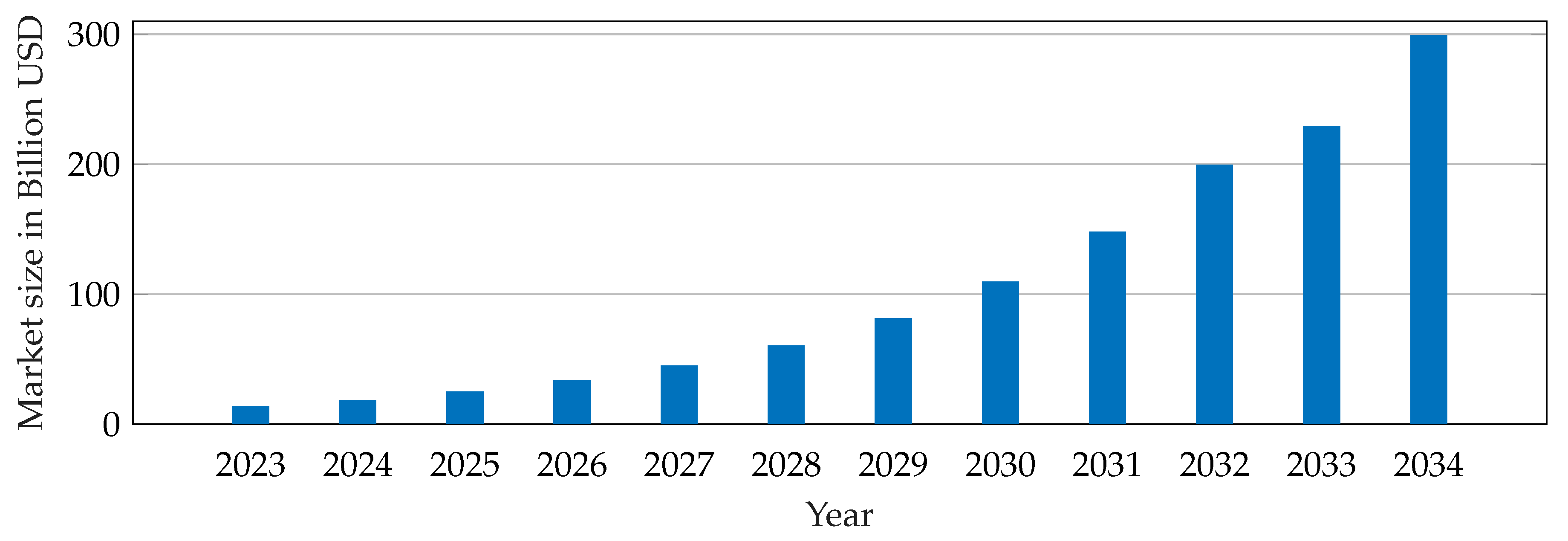
Figure 2.
An illustration of a waveform-agnostic transmission and reception process in automotive radars is shown. Green indicates transmitted pulses, each lasting , within the CPI of duration , transmitted at intervals of . Orange shows received echoes from multiple target reflections, repeated over a cycle .
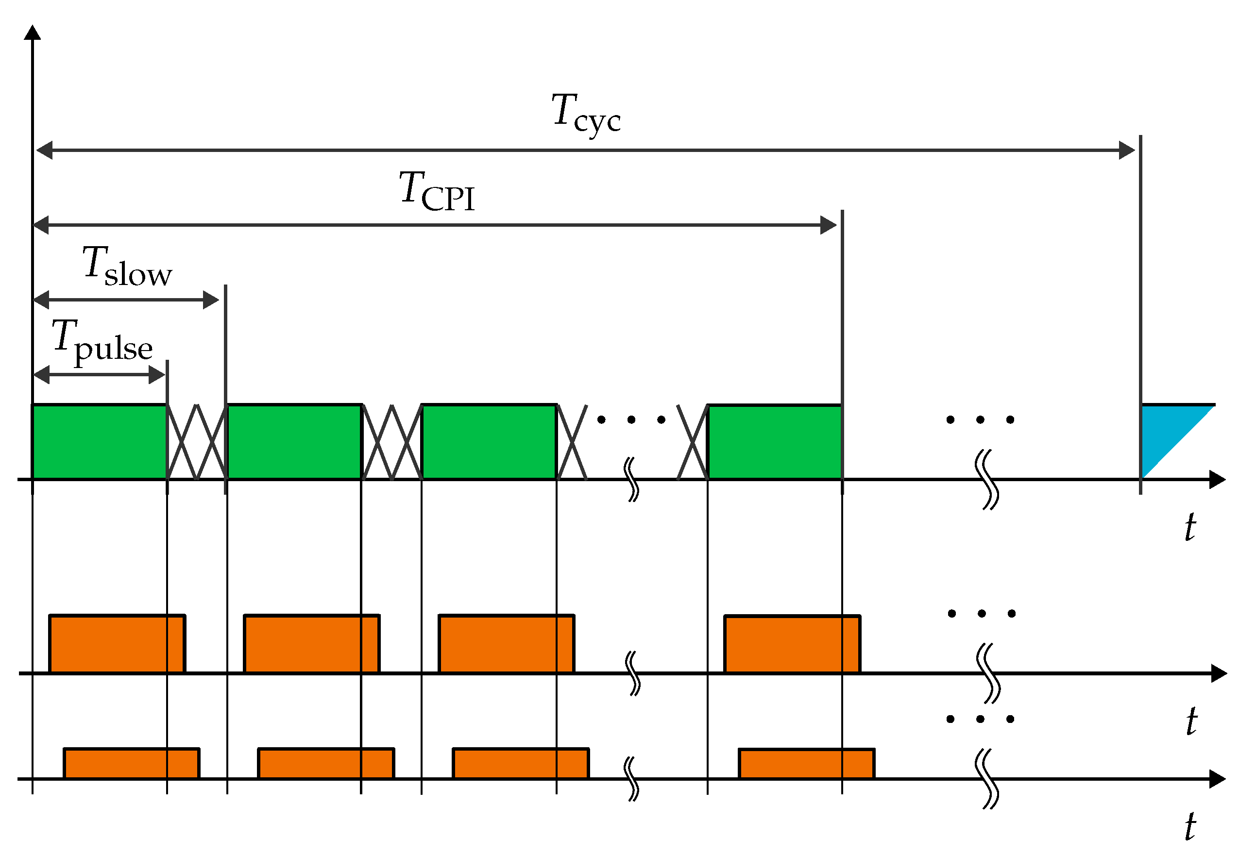
Figure 3.
A linear chirp FMCW waveform in two representations. (a) Time domain representation. (b) Frequency over time with , where is the starting frequency and is the slope of chirp with the swept bandwidth and the pulse duration .
Figure 3.
A linear chirp FMCW waveform in two representations. (a) Time domain representation. (b) Frequency over time with , where is the starting frequency and is the slope of chirp with the swept bandwidth and the pulse duration .
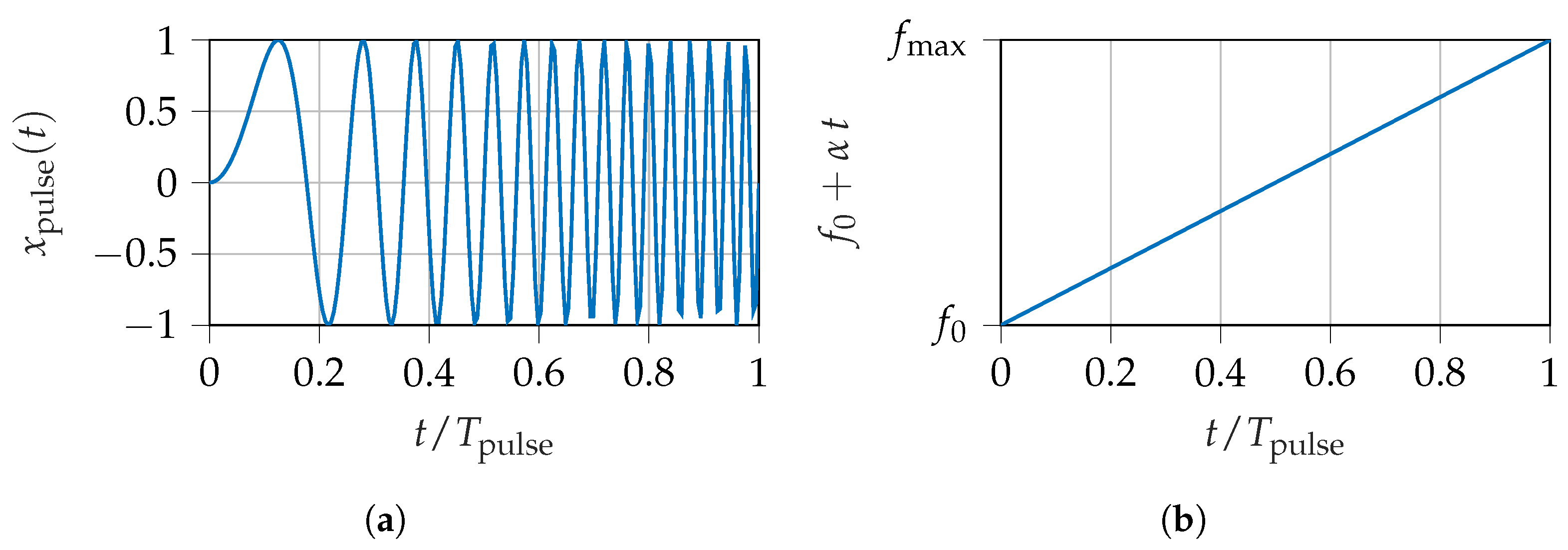
Figure 4.
A block diagram of a SISO-FMCW radar system. Green denotes RF-bandwidth signals, orange denotes IF-bandwidth signals. At the receiver, the transmitted and received signals mix to produce a low-frequency beat.
Figure 4.
A block diagram of a SISO-FMCW radar system. Green denotes RF-bandwidth signals, orange denotes IF-bandwidth signals. At the receiver, the transmitted and received signals mix to produce a low-frequency beat.
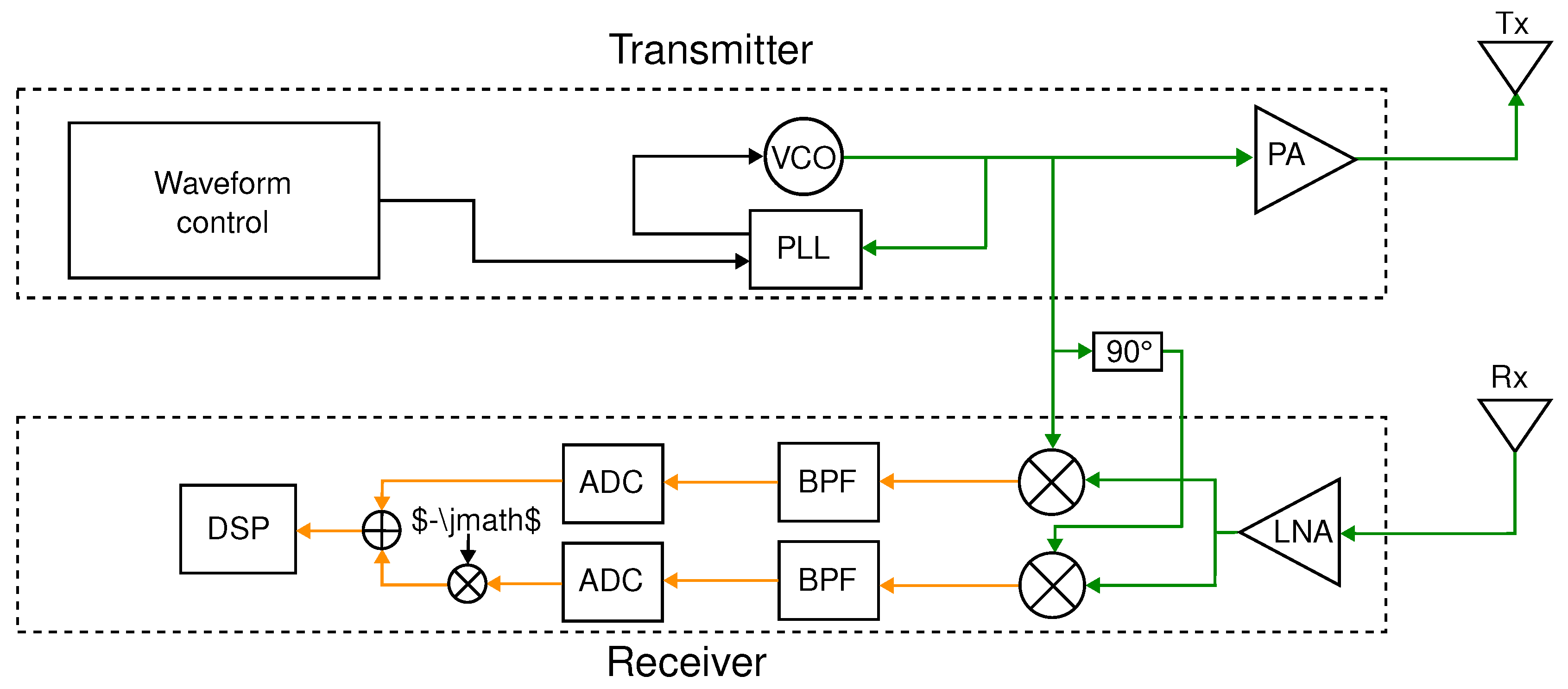
Figure 5.
A PMCW waveform in two representations: Orange shows the pulse waveform , and blue shows the modulated RF waveform . The pulse is the analog representation of a 8-chip binary sequence.
Figure 5.
A PMCW waveform in two representations: Orange shows the pulse waveform , and blue shows the modulated RF waveform . The pulse is the analog representation of a 8-chip binary sequence.
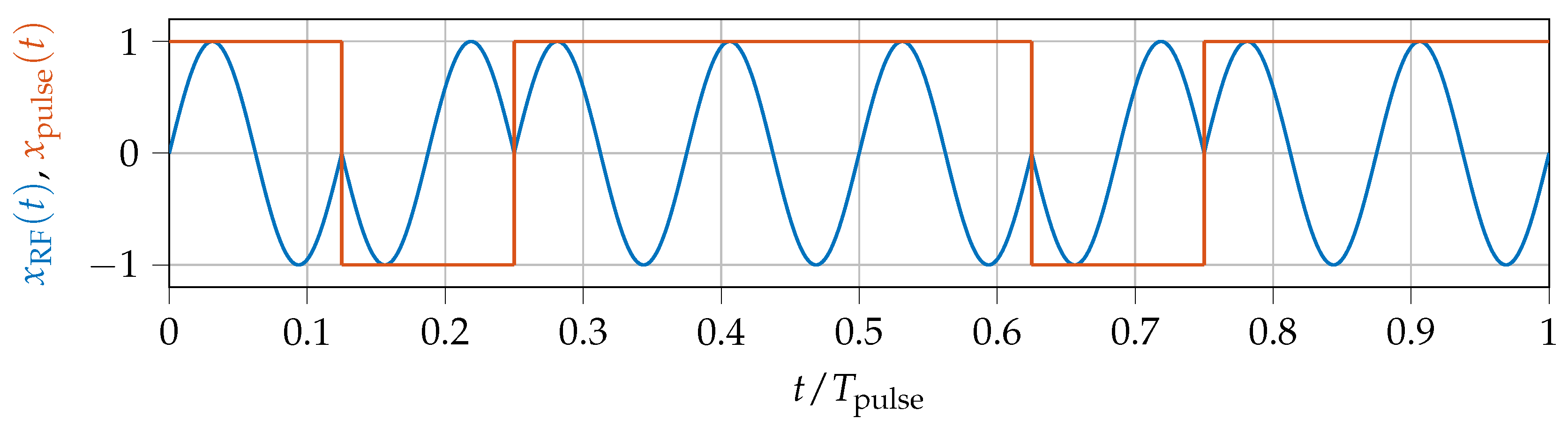
Figure 6.
A block diagram of a SISO-PMCW radar. The green color indicates signals with RF bandwidth. The instantaneous pulse bandwidth equals the receiver-side bandwidth after demodulation, thereby requiring fast-sampling ADC.
Figure 6.
A block diagram of a SISO-PMCW radar. The green color indicates signals with RF bandwidth. The instantaneous pulse bandwidth equals the receiver-side bandwidth after demodulation, thereby requiring fast-sampling ADC.
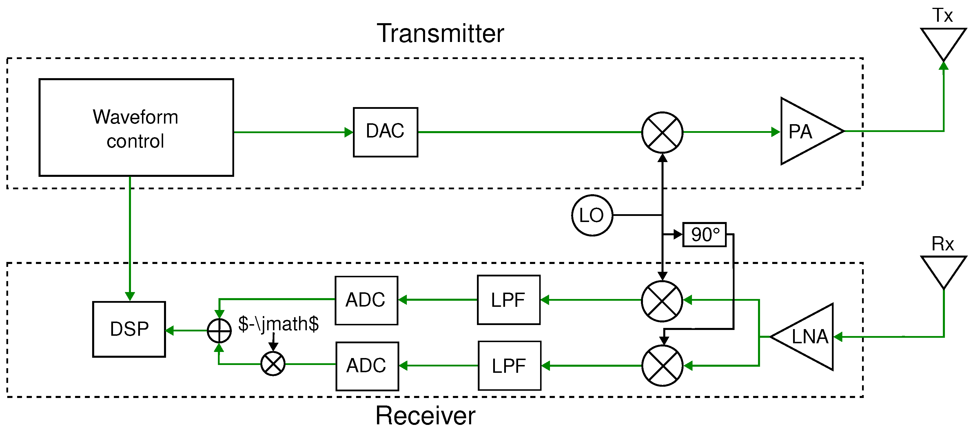
Figure 7.
A PC-FMCW waveform in two representations. Blue shows the chirp signal , and orange indicates a phase code . The phase change of is determined by .
Figure 7.
A PC-FMCW waveform in two representations. Blue shows the chirp signal , and orange indicates a phase code . The phase change of is determined by .
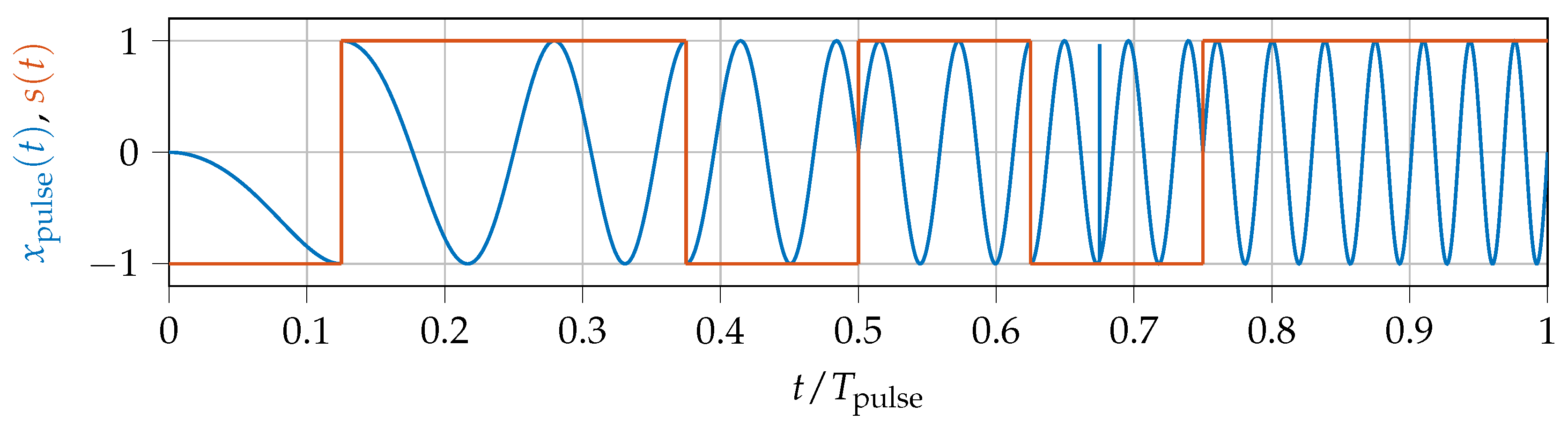
Figure 8.
A block diagram of a SISO-PC-FMCW radar from [7] is shown. Green denotes signals with RF bandwidth, and orange represents signals with IF bandwidth. At the transmitter, a coder applies a phase code to the chirp signal. The receiver’s GDF delays frequency components based on their beat frequencies to the maximum delay. The decoder then removes the phase code.
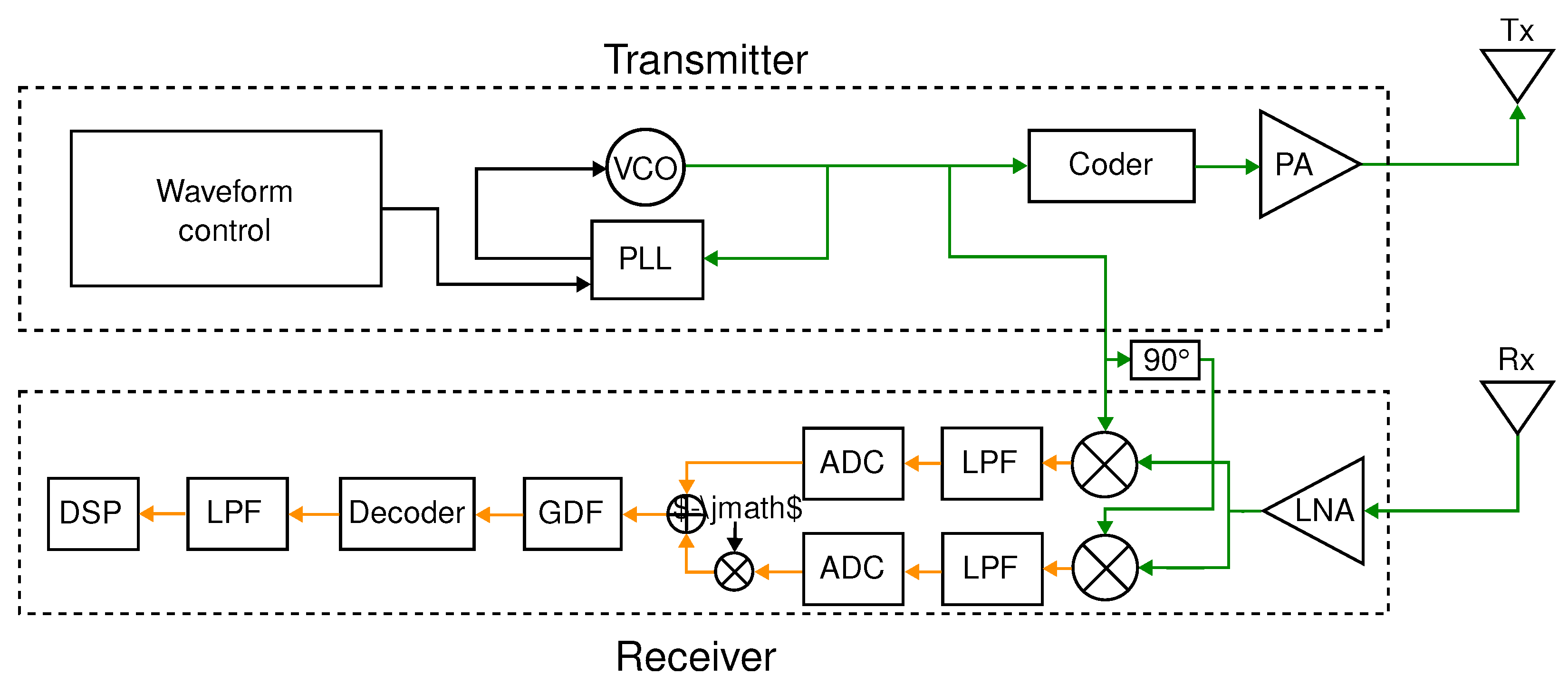
Figure 9.
Illustrations of the OFDM waveform in two representations. Varied colors represent distinct carrier frequencies. (a) In-phase (solid) and quadrature (dashed) components of the orthogonal subcarriers, where is defined in (28). (b) Orthogonal subcarriers in the frequency domain representation. The subcarrier spacing is defined as .
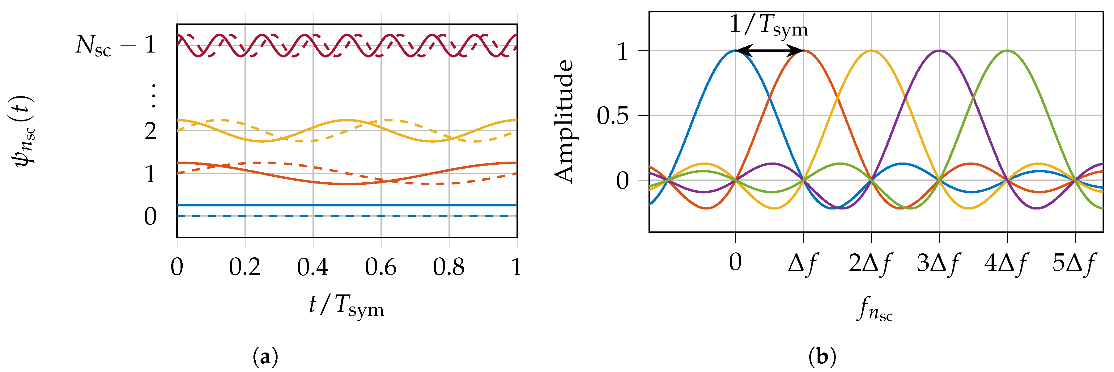
Figure 10.
A block diagram of an SISO-OFDM radar. Green indicates signals with RF bandwidth.
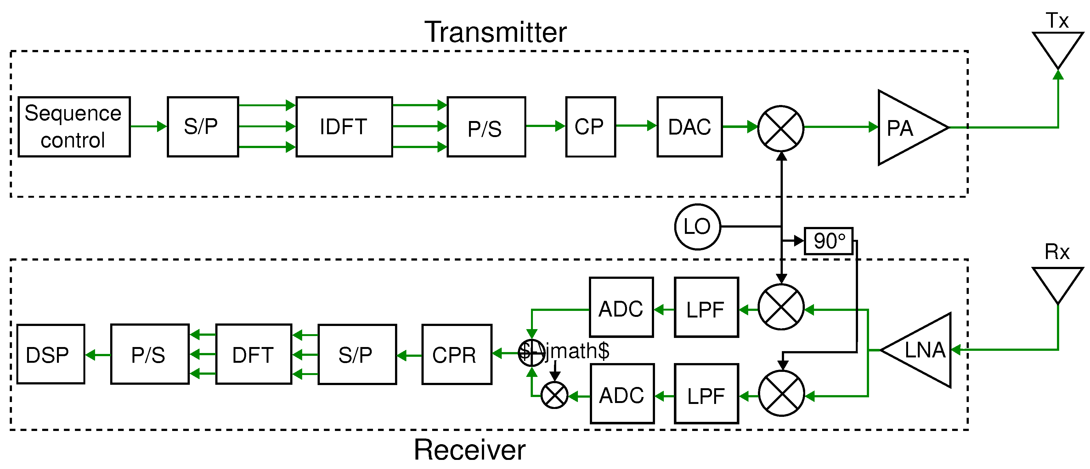
Figure 11.
Illustrations of the OCDM waveform in two representations. Varied colors represent distinct subchirps. (a) In-phase (solid) and quadrature (dashed) components of the orthogonal chirp waveforms, where is defined in (33). (b) Orthogonal chirps in the time-frequency domain.
Figure 11.
Illustrations of the OCDM waveform in two representations. Varied colors represent distinct subchirps. (a) In-phase (solid) and quadrature (dashed) components of the orthogonal chirp waveforms, where is defined in (33). (b) Orthogonal chirps in the time-frequency domain.
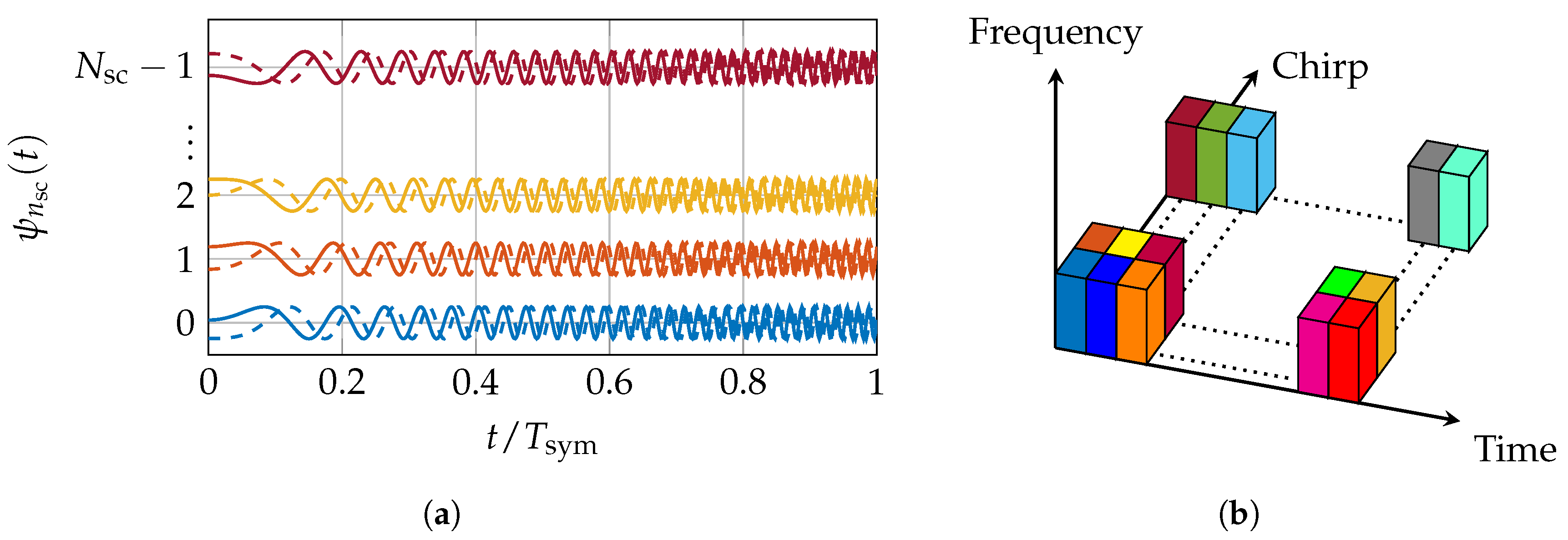
Figure 12.
A block diagram of an SISO-OCDM radar. Green indicates signals with RF bandwidth.
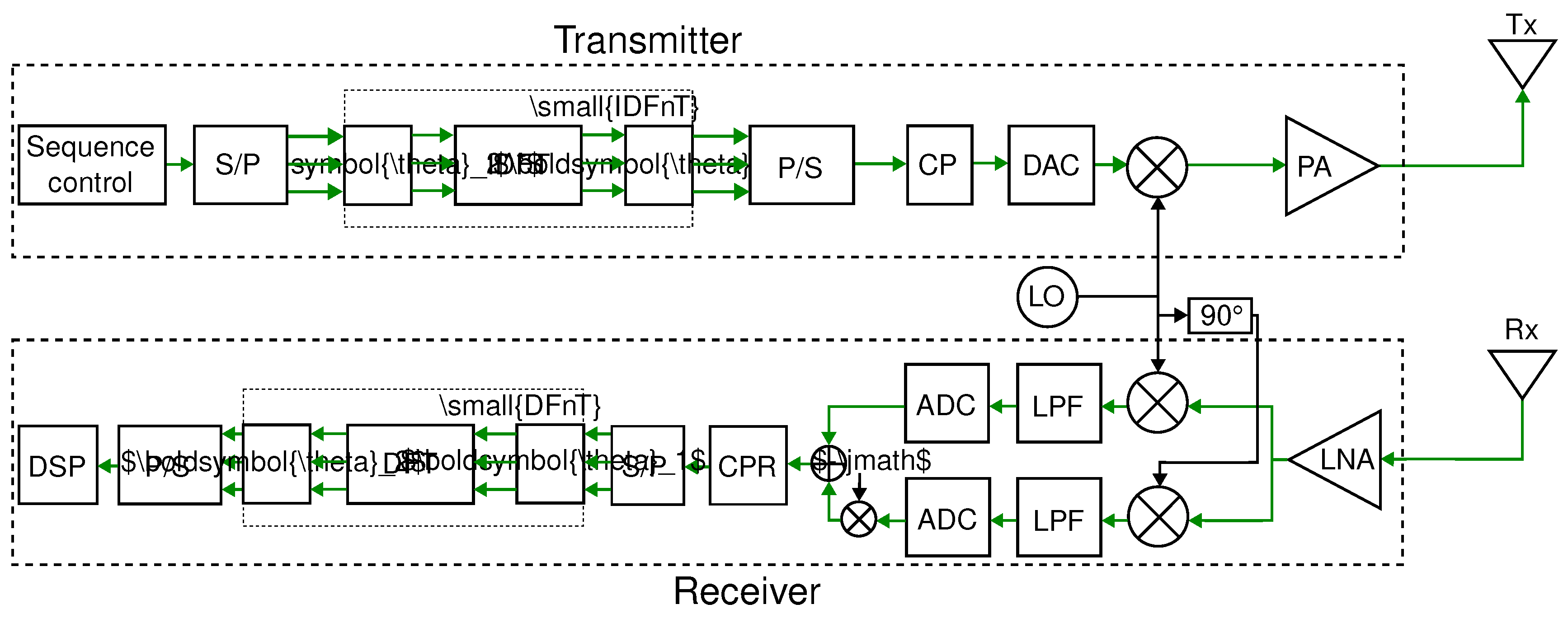
Figure 13.
A block diagram of an SISO-OTFS radar. Green indicates signals with RF bandwidth.

Figure 14.
Illustration of an observation scenario on a highway. There are six road users with individual radar system settings. Cars A and E are equipped with eight radars each, while car F, for example, has only two radars. An overhead sign gantry is present, which is a challenge for a conventional radar without elevation measurement capability.
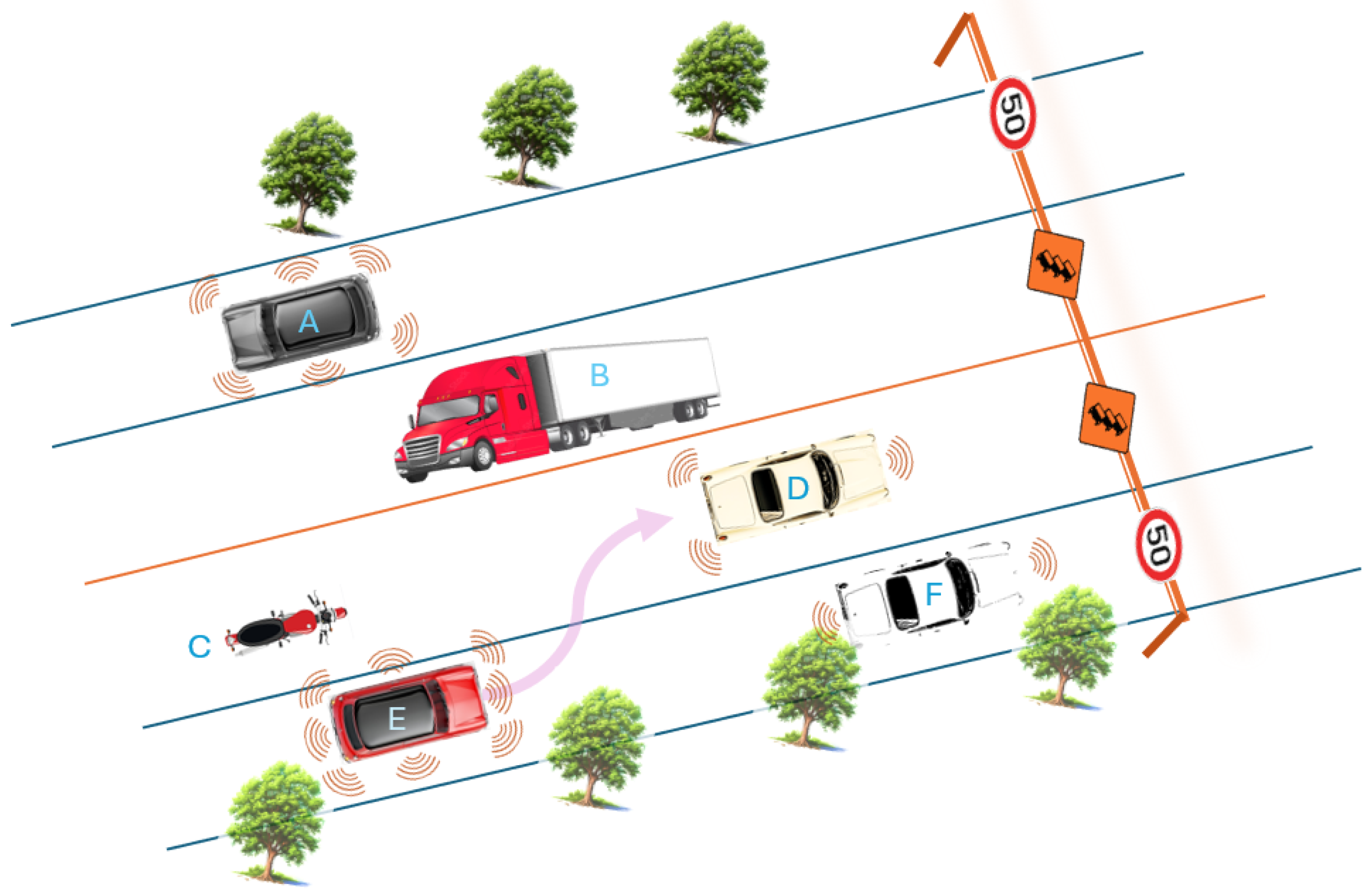
Figure 15.
Blue: victim radar chirps; green: object echo; red: aggressor radar chirp; dashed: LPF bounds. (a) FMCW chirps with differing parameters interfere in the time–frequency domain (black circle: intersection of victim and aggressor chirps). (b) Baseband beat signal of the real echo overlapped by interference.
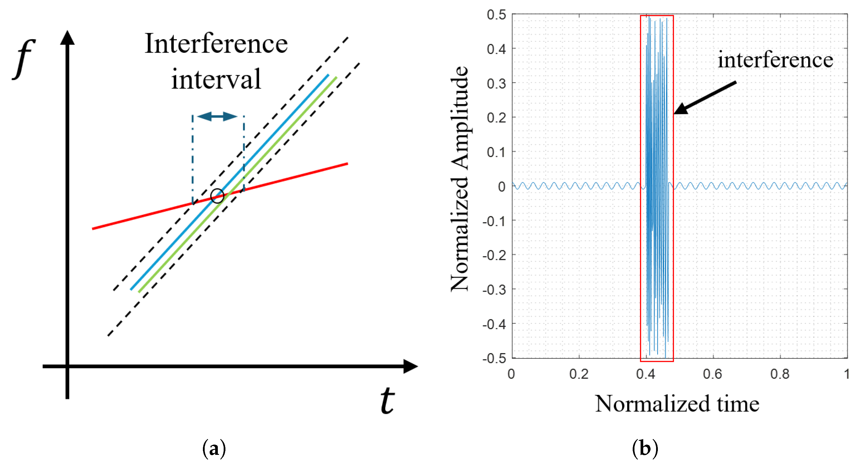
Figure 16.
Based on [11], the RD spectrum in (a) shows multiple point targets without interference, while (b) shows the same scene with interference.
Figure 16.
Based on [11], the RD spectrum in (a) shows multiple point targets without interference, while (b) shows the same scene with interference.

Figure 17.
(a) A visualization of the interference between chirps with identical PRI, where the chirps from the aggressor are highlighted in magenta. (b) The interfered RD spectrum corresponding to (a). The same case as in (a) is shown in (c), but aggressor’s PRI is shorter. (d) The interfered RD spectrum corresponding to (c).
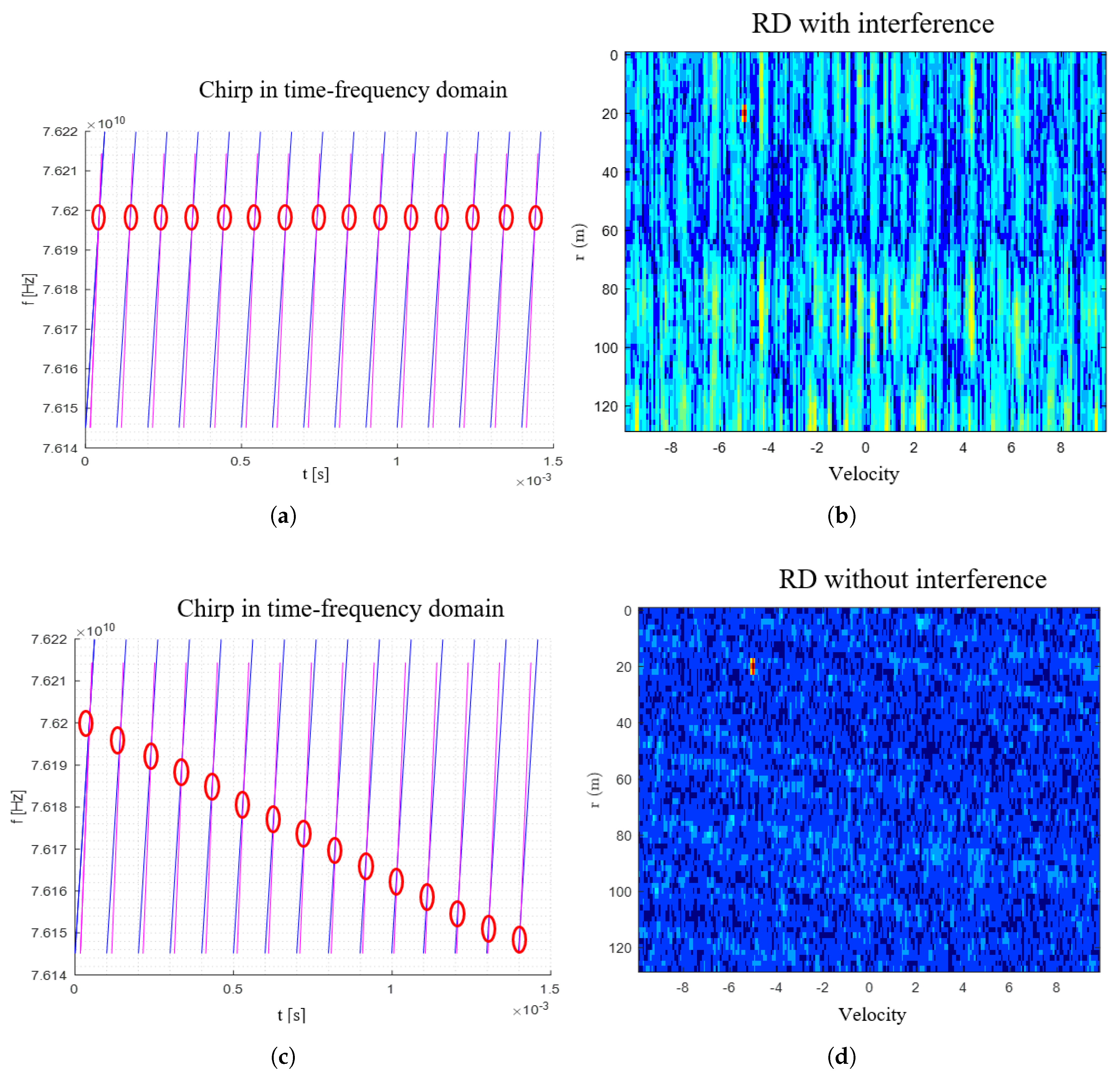
Figure 18.
Interference simulation of FMCW versus PC-FMCW provided in [24]. The axis description is modified according to this work. The red lines denote the interference. The Dirac delta peaks are attributed to phase coding in the waveform of PC-FMCW.
Figure 18.
Interference simulation of FMCW versus PC-FMCW provided in [24]. The axis description is modified according to this work. The red lines denote the interference. The Dirac delta peaks are attributed to phase coding in the waveform of PC-FMCW.
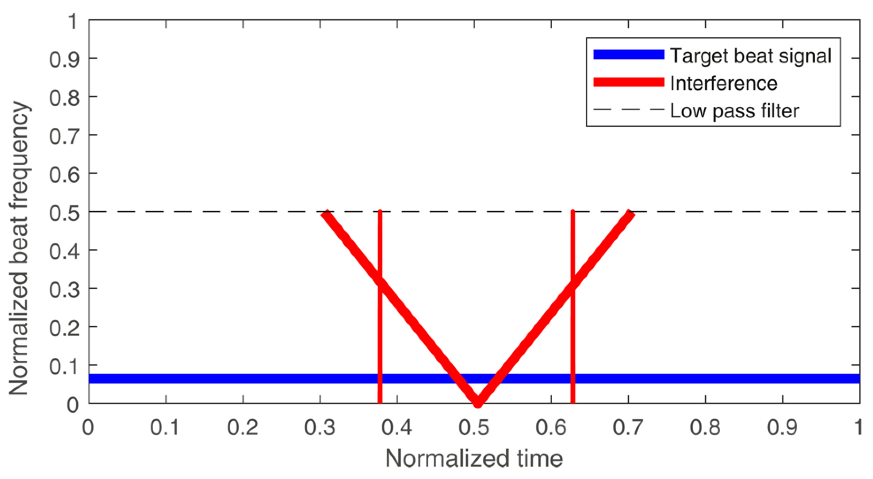

Table 1.
An overview of related works and their contributions.
| Modulation | Ref. | Year | Authors | Title | Contribution | |||||
|---|---|---|---|---|---|---|---|---|---|---|
| FMCW | PMCW | PC-FMCW | OFDM | OCDM | OTFS | |||||
| × | × | × | [6] | 2021 | Waldschmidt et al. | Automotive Radar — From First Efforts to Future Systems | Review of radar development over years with a focus on research topics of automotive radar such as digital modulation schemes, radar networks, radar imaging, and machine learning. | |||
| × | × | × | [21] | 2023 | Giuffrida et al. | A Survey of Automotive Radar and Lidar Signal Processing and Architectures | Review of radar and lidar technology with a focus on modulation schemes and imaging systems, highlighting weaknesses and strengths and presentation of sensor fusion concepts | |||
| × | × | × | [22] | 2019 | Hakobyan et al. | High-Performance Automotive Radar: A Review of Signal Processing Algorithms and Modulation Schemes | Review of modulation schemes with a focus on signal processing and interference mitigation. | |||
| × | × | × | × | [23] | 2017 | Patole et al. | Automotive radars: A review of signal processing techniques | Review of aspects, such as waveform design, architectures, estimation algorithms, implementation complexity-resolution, processing for complex environments, and unique problems associated with automotive radar. | ||
| × | × | × | [24] | 2021 | Kumbul et al. | Automotive radar interference study for different radar waveform types | Interference study on different waveforms and experimental demonstration of PC-FMCW waveforms. | |||
| × | × | × | × | [25] | 2020 | Carvajal et al. | Comparison of Automotive FMCW and OFDM Radar Under Interference | Performance comparison of FMCW and OFDM in terms of interference. The results show that both waveforms can perform similarly under proper windowing, but OFDM is more sensitive to interference. | ||
| × | × | × | × | [17] | 2021 | Schweizer et al. | The Fairy Tale of Simple All-Digital Radars: How to Deal With 100 Gbit/s of a Digital Millimeter-Wave MIMO Radar on an FPGA | Implementation of PMCW and OFDM modulation on Xilinx RFSoC FPGA with performance demonstration, showing that sophisticated digital design is required to realize the radar processing. | ||
| × | × | × | [12] | 2019 | Roos et al. | Radar Sensors for Autonomous Driving: Modulation Schemes and Interference Mitigation | Presentation of modulation schemes and interference mitigation for automotive radar, namely FMCW, PMCW, and OFDM. | |||
| × | [26] | 2016 | Giroto de Oliveira et al. | Joint Radar-Communication Systems: Modulation Schemes and System Design | Overview of modulation schemes for JRC systems with detailed systems models and parameters for quantifying radar and communication performance. | |||||
Table 2.
An Overview of Waveform-Specific Symbol Notations.
| Modulation | Bandwidth | Number of pulses | Pulse duration | Slow-time interval |
|---|---|---|---|---|
| Agnostic | B | |||
| FMCW | ||||
| PMCW | ||||
| PC-FMCW | ||||
| OFDM | ||||
| OCDM | ||||
| OTFS |
: swept chirp bandwidth, : chip bandwidth, : subcarrier-spanned bandwidth, : number of accumulations, : number of chips, : number of chirps, : number of sequences, : number of subcarriers, : number of symbols, : cyclic prefix interval, : chip duration, : chirp duration, : idle time, : sequence duration, : symbol duration, : subcarrier spacing.
Table 3.
System Parameters for FMCW, PMCW, PC-FMCW, OFDM, OCDM, and OTFS Modulation Schemes.
| Waveform | Range resolution | Unambiguous range | Velocity resolution | Unambiguous velocity |
|---|---|---|---|---|
| FMCW | ||||
| PMCW | ||||
| PC-FMCW | ||||
| OFDM | ||||
| OCDM | ||||
| OTFS |
: chirp bandwidth, : sampling rate, : number of accumulations, : number of chips, : number of chirps, : number of subcarriers, : number of sequences, : number of symbols, : cyclic prefix interval, : chip duration, : chirp duration, : idle time, : sequence duration, : symbol duration, : subcarrier spacing.
Table 4.
Essential Features for FMCW, PMCW, PC-FMCW, OFDM, OCDM, and OTFS Modulation Schemes.
| Parameter | FMCW | PMCW | PC-FMCW | OFDM | OCDM | OTFS |
|---|---|---|---|---|---|---|
| Modulation | Analog | Digital | Analog + Digital | Digital | Digital | Digital |
| Multiplexing | TDM / DDM | CDM | CDM | FDM | chirp / FDM via FSP / CDM | delay-Doppler |
| Communication | proof-of-concepts available | high-speed communication possible | low-speed communication possible | high-speed communication possible | high-speed communication possible | high-speed communication possible |
| Interference | susceptible | susceptible | susceptible | susceptible | N/A | N/A |
| Doppler tolerance | good — range-Doppler coupling | low — decreased PSR after range processing | good — range-Doppler coupling | low — loss of subcarrier orthogonality | good — loss of subchirp orthogonality | good — native |
| Implementation | simple, but linear frequency synthesizer required | fast-sampling ADC required + a large amount of data must be stored and processed | simple, but linear frequency synthesizer and additional components compared to FMCW are required | high PAPR + synchronization for decoding required + fast-sampling ADC required + large amount of data must be stored and processed | reduced PAPR compared to OFDM possible + integration/coexistence with OFDM system possible | reduced PAPR compared to OFDM possible |
| Range processing | DFT | Correlation | DFT | IDFT | IDFT | Wigner transform + SFFT |
| Doppler processing | DFT | DFT | DFT | DFT | DFT | Wigner transform + SFFT |
| ADC rate | slow — less than | fast — up to | mid — less than | fast — up to | fast — up to 4 | fast — up to 4 |
| Cost | cost-efficient | expensive | cost-efficient | expensive | expensive | expensive |
| Status | mature in industry | started in industry | academia | academia | academia | academia |
Disclaimer/Publisher’s Note: The statements, opinions and data contained in all publications are solely those of the individual author(s) and contributor(s) and not of MDPI and/or the editor(s). MDPI and/or the editor(s) disclaim responsibility for any injury to people or property resulting from any ideas, methods, instructions or products referred to in the content. |
© 2025 by the authors. Licensee MDPI, Basel, Switzerland. This article is an open access article distributed under the terms and conditions of the Creative Commons Attribution (CC BY) license (http://creativecommons.org/licenses/by/4.0/).
Copyright: This open access article is published under a Creative Commons CC BY 4.0 license, which permit the free download, distribution, and reuse, provided that the author and preprint are cited in any reuse.


