
Submitted:
19 March 2025
Posted:
20 March 2025
You are already at the latest version
Abstract
The optimization of rocket nozzle design remains critical for advancing the efficiency and performance of space propulsion systems. This investigation presents an in-depth analysis of supersonic nozzle configurations and their aerodynamic behaviors, with a specific focus on methodologies to design a contour capable of enhancing thrust by reducing losses under. Further concepts of compressible aerodynamics and CFD are also reported, compassing the state of the art in chapters 1 and 2 necessary to base the studies reported. Chapter 3 investigates traditional nozzle designs, specifically conical and bell nozzles, employing the Method of Characteristics (MOC) to compute their flow characteristics and optimize geometrical parameters for minimum length and maximum thrust efficiency. Various design contours, including parabolic and truncated ideal configurations, are evaluated for their applicability in diverse applications such as supersonic wind tunnels and propulsion systems.In Chapter 4, the research extends to advanced nozzle geometries, including aerospike, dual-bell, expansion-deflection, and multi-grid nozzles, each offering unique advantages in adapting to varying pressure environments. These designs are analyzed for their ability to mitigate under- and over-expansion losses, improved thrust coefficient, and enhance specific impulse. The studies emphasize the critical balance between design complexity, manufacturing constraints, and aerodynamic performance, establishing guidelines for integrating innovative design features into modern propulsion systems.Computational simulations and theoretical formulations underscore the effectiveness of improved MOC techniques and boundary-layer corrections in accurately predicting nozzle performance. The findings have broad implications for the development of propulsion systems in high-demand applications, including single-stage-to-orbit (SSTO) vehicles and hypersonic flight systems.
Keywords:
Method of Characteristics
; Nozzle Design
; Compressible Aerodynamics
; Nozzle Contour
; CFD (Computational Fluid Dynamics)
1. Introduction
1.1. History of Rocket Propulsion
Rockets and their fundamentals have been around humankind history for a while, with their bigger developments being associated with warfare. Starting as bamboo tubes filled with gunpowder used in religious celebrities, primitive rockets are invented in the 1st century China. “Arrows of flying fire”, resembling solid propellant rockets, are the first warfare application of rocket propulsion, used in 1232 by the Chinese army to repel the Mongol invaders.
It is during the 20th century that rocketry is heavily developed into almost nowadays technology, being encourage by the needs of World War Two and the Cold War.
Robert H. Goddard, an american engineer, designs and builds the first liquid propellant rocket. 34 rockets where launch between 1926 and 1941, getting to altitudes of up to 2.6 km and speeds as high as 885 km/h. Later, in 1945, the single and multi-stage rocket engines for both rocket and jet-assisted takeoff are developed by Goddard.
During the same time, german engineer Wernher von Braun develops the V-2, a liquid-propellant rocket missile used by the Axis Forces in World War Two. In the after math of the war, von Braun is recruited by NASA becoming a prominent figure in the developing of the Saturn V launcher.
During the height of the Space Race, driven by the Cold War, the development of rocket technology reached its peak, resulting in several notable milestones[1]:
- 1957 – The launch of the first Earth-orbiting artificial satellite, Sputnik I, by the USSR. The satellite Sputnik II carried a dog named Laika into orbit, later that year.
- 1959 – The lunar surface is firstly touched by a human-made object, the USSR’s Luna 2
- 1961 – Venus is first flew by the USSR’s Venera 1, being the first to reach another planet.
- 1962 – Yuri Gagarin is the first human in space onboard the USSR’s Vostok spacecraft.
- 1969 – The American Apollo 11, powered by Saturn V rockets, successfully landed the first humans on the moon, Neil Armstrong and Buzz Aldrin.
- 2013 – Voyager 1, launched in 1977 by the USA, becomes the first human-made object to leave the solar system.
Nowadays, several nations like Europeans countries (under ESA), India, Japan, China, Brazil, among many others, have their own space programs, for which rockets, and their development, are crucial. Even more recently, the space industry stopped being a centralized state research to become also a private business, as recent Space X, Blue Origin and Virgin Galactic launches prove.
2. De Laval Convergent-Divergent Nozzle
Thrust is generated in aerial vehicles by mass ejection, as per Newton’s third law, mathematically by the simplified Equation 1. Besides the first parcel of the Equation corresponding to mass ejection, a second force is generated by the pressure difference between the flow at the exit and the ambient pressure, translated in the second parcel [1].
Nozzles where invented as means to change the properties of a flow such as velocity and pressure. The de Laval nozzle, containing a convergent followed by a divergent section does so in such a way that a supersonic flow can be obtain at the exit. The flow behavior off such nozzle is observed in Figure 1.
A de Laval nozzle is composed of three sections: the convergent (subsonic), the throat (sonic) and the divergent (supersonic). In each regions, the flow behaves differently, with differentiated analysis methods to determinate its contribution for the production of thrust.
The convergent section accepts the hot and higly pressured exhaust gases from the combustion chamber, at almost static conditions, providing the first mean of acceleration until a sonic value. So, the convergent affects the mass flow and, at some degree, the efficiency of the combustion chamber.
At the throat, the flow reaches a sonic velocity, being choked, meaning it can not be accelerated further without area increases. Having a fixed area and Mach Number, it’s the throat, and flow’s properties dependent upon the conditions provided by the combustion chamber, that limits the mass flow through the nozzle, posing great impact on the thrust produced according to the first parcel of Equation 1.
The same parcel of thrust’s Equation 1, is also greatly impacted by the exit velocity. Since the flow is choked at the throat, is in the divergent section that accelerates it further to supersonic values. The comprehensible flow keeps on gaining kinetic energy as a trade off by losing internal energy (as seen in Figure 1 by the decrease in temperature), with a pressure drop. The exit velocity is dependent on the ratio between exit and throat areas, outside conditions in relation to the chamber and the divergent section design that affects the flow’s orientation and can induce losses.
Three major concepts are necessary to evaluate a nozzle’s performance. The first concept, represented by Equation 2, is the specific impulse, which measures the thrust produced by the weight flow rate of propellant burned. It is important to understand the rocket’s nozzle efficiency.
The second concept, represented by Equation 3, is the total impulse, which measures the thrust produced over the entire duration of the engine’s operation.
Finally, the thrust coefficient, exhibited in Equation 4, represents the dimensionless value of thrust obtained by dividing it by the chamber pressure and the throat area. This is a fair indicator of nozzle efficiency since, in theory, the thrust value depends solely on the pressure ratio between the chamber and the ambient, and the area ratio between the exit plane and the throat [3].
2.1. Ideal Nozzle
The ideal nozzle is a concept that provides the best theoretical performance for the given conditions, to which all nozzle designs are compared to. A parallel flow and exit pressure matching external pressure are some consequences from this simplification. Looking into more detail, the ideal nozzle involves the following considerations [3]:
- The exhaust gases are in chemical equilibrium, with a homogeneous composition and in a gaseous state.
- The exhaust gases obey the perfect gases law.
- The flow is adiabatic, meaning there are no appreciable heat transfers to the wall.
- The flow is isentropic, without discontinuities in properties and/or shock waves.
- The boundary layer effects are neglected, with no wall friction decelerating parts of the flow.
- The flow rate is constant and steady, without gas pulsations, turbulence, and with the transient effects of starting-up and shutting down neglected since they are of short duration.
- The exit flow is parallel and uni-dimensional.
- The flow’s velocity, pressure, temperature, and density are uniform across any nozzle’s normal section.
- Before the combustion process, propellants are store at ambient temperature, except for cryogenics which are at their boiling point.
Nonetheless, this are fair simplifications due to how fast the expansion occurs. For chemical rockets, tested efficiency parameters are usually just 1%-6% below those calculated with totally ideal assumptions [3].
3. Real Nozzle
The level of precision required for rocket systems and to optimize an already very efficient system, demands more accurate algorithms that involve a better understanding of energy losses, heat transfer and other physical or chemical phenomena.
In real nozzles, not all the chemical energy contained in the propellant is available as thermal energy, and not all the thermal energy can be converted into kinetic energy. Therefore, the performance of a rocket nozzle is affected by several factors and non-idealities that can cause losses in thrust and specific impulse.
The first factor, already stated before as a concern, is the divergency losses resulting from a non-unidimensional flow profile at the exit plane due nozzle contours that don’t end in a null slope. Another factor is that small chamber areas relative to the throat, lead to pressure losses in the chamber and a reduction of the exhaust exit velocity and thrust produced.
Boundary layer effects can also be significant, particularly for smaller nozzles with low area ratios, making a portion of the flow, ranging from to , subsonic. Due to the no-slip condition, the flow next to the wall has zero-speed with high thermal energy that is dissipated to the wall and the nearby moving flow. The immediate flow is laminar and subsonic, turning further from the wall into transonic/supersonic zones where turbulence can occur, before it joins the totally supersonic free stream.
Combustion in the rocket propulsion is typically unsteady, resulting in flow oscillations and lower chamber pressure during transient operations. Chemical reactions in the flow can cause losses of up to , and incomplete mixing of the gas composition means that the gas constants are not uniform throughout the nozzle, contributing for some mathematical incongruities of the numerical models.
Small solid particles and liquid droplets also exist in the flow, which need to be accelerated, with little thermal energy contribution. If bigger than 0.015mm and equivalent to more than 6% of the flow’s mass, specific impulse losses can rise to -. Although less significant, in high area ratio nozzles, aggressive expansion can lead to the precipitation of some exhaust constituents.
It still must be mentioned that uncooled materials suffer erosion, a phenomena of upmost relevance for the throat since, if its area increases, some chamber pressure is lost, with an additional area ratio decrease. Up to of specific impulse can be lost.
And, at last, operating away from the design altitude reduces thrust and specific impulse for nozzles with fixed area ratio [3].
4. Nozzle Phenomena
4.1. Operation Critical Points
Fixing the chamber pressure, flow begins in subsonic regime throughout the entire nozzle when the outside pressure starts to drop, expanding in the divergent and xompressing in the divergent. As the pressure ratio () increases, the flow accelerates and the mass flow rate rises until it reaches a sonic value at the throat, causing the flow to choke. Beyond the throat, the flow keeps compressing in the divergent section, and it returns to a subsonic regime. This point is called the first critical point and is represented in Figure 2 by curve a. Any infinitesimal decrease in the outside pressure beyond the first critical point will cause the flow in the divergent section to change from subsonic to supersonic.
Now that there is a supersonic flow in the divergent section, it no longer compresses but expands, but the great area variation promotes a more aggressive expansion than the one needed to equal the ambient pressure. Thus, a shock forms inside the divergent section, starting at the throat and moving to the exit plane as the outside pressure drops and a non-isentropic compression besides the shock is needed so, after the shock, the flow becomes subsonic and uses the remaining divergent section as a compressor. This is represented by line b in Figure 2. When the outside pressure is low enough, the shock reaches the exit plane, as suggested by line c in the same figure, representing the second critical point.
After the second critical point, the flow will not be able to expand much further even if the ambient pressure keeps dropping. However, it still reaches the exit plane at higher pressures than the ambient. Therefore, the normal shock at the exit begins to turn oblique, with its intensity/angle reducing as the outside pressure decreases. This phenomenon is known as an overexpanding nozzle.
The oblique shock will eventually reach a angle, representing no shock at all, and the nozzle reaches its third critical point. At this point, the flow is isentropic and is used as the nozzle’s design point.
Further decreases in outside pressure will cause the flow to have a pressure higher than the ambient pressure at the exit, which is known as underexpansion. In this case, expansion fans will be generated from the nozzle’s lips to allow the flow to be further expanded beyond the exit plane.
4.2. Overexpansion and Underexpansion Phenomena
The overexpansion occurs when the ambient pressure is higher than the one at the third critical point. A weak shock is needed at the exit so that the flow pressure increases until it matches the ambient pressure.
But the oblique shock will deviate the flow, so a second shock is needed to realign the flow. This will increase the pressure, making it higher than the ambient pressure, so now an expansion fan is needed to expand the flow and match the ambient pressure once again.
The expansion fan also deviates the flow, requiring another expansion fan to straighten the flow, returning it to a state where its pressure is again below the ambient pressure.
5. Theory of Flow in Nozzles
6. Introduction to High Velocity Compressible Flow
When a flow subjected to great gradients and accelerates to high velocities from stagnation, density cannot be assumed to be constant raising the concept of compressible flow. Examining Equation 5, if the pressure experienced by a finite volume of fluid increases, compression occurs, resulting in a reduction in volume and an increase in density. The symbol represents the compressibility of the gas, which has different values for isothermal and isentropic processes.
High-speed flows are often initiated and propelled by strong pressure gradients. Therefore, the impact of pressure on the gas density cannot be ignored. Equation 6 relates the three main properties for any two states in a gaseous flows assuming isentropy. [6].
6.1. Speed of Sound and Mach Number
All particles within a fluid move in random directions with a certain velocity, attributing the fluid a specific internal energy. This random kinetic propagation speed is known as the speed of sound, and it is dependent on the fluid and its internal energy, as described by Equation 7 for thermally and calorically perfect gases. When a perturbation is applied to the fluid, it will excite nearby molecules, which will eventually collide with other molecules, transmitting the disturbance at a specified mean speed.
The Mach number is defined as the ratio between the velocity of the flow and the velocity of sound, as shown in Equation 8. It represents the relationship between the flow’s kinetic energy and the random molecular kinetic energy. Based on it, different flow regimes can be established, including:
- Incompressible (M < 0.3) – Density variations are small, mostly because these flows are not associated with strong pressure gradients. Hence, this flow can be assumed to possess constant density.
- Subsonic (0.3 < M < 0.8 at freestream) – Property variations are always continuous, and the flow exhibits straight and parallel streamlines that move, converge and shape around any obstacle. In every point, the flow has a Mach number less than 1, but compressibility effects cannot be ignored.
- Transient (0.8 < M< 1.2) – As the flow approaches the speed of sound, it is not possible to guarantee that all the flow is subsonic since it may accelerate while contouring an object, creating supersonic "pockets." Shocks can appear, indicating discontinuous changes in properties.
- Supersonic (M > 1) – The entire flow moves faster than the speed of sound. Streamlines do not bend around objects, except when encountering a shock or experiencing an expansion wave. After a shock, the flow must remain supersonic.
- Hypersonic (M > 5) – At such high speeds, a shock wave causes explosive changes in properties. The temperature can increase so much that molecular dissociation effects must be considered. Nothing particularly special happens at M = 5, as the referred phenomenon increases with the Mach number, being just a convention.
The Mach number allows the calculation of the Mach Angle, as shown in Equation 9, which is half of the Mach Cone’s angle. This structure is formed by pressure waves and appears around bodies moving faster than the speed of sound. To be noted that the outside of the Mach Cone is called the silence zone, where the presence of a moving object cannot be heard.
6.2. Stagnation Properties
All motion is described in relation to a reference frame. In compressible flow, an isentropic deceleration can be implemented until the flow becomes static in relation to such reference frame. The new values of the fluid’s properties are called total or stagnation properties, identified with the suffix “0”. In a rocket’s nozzle, this reference state is the conditions felt at the combustion chamber, as velocity is so small compared to that at the nozzle, so it can be overlooked.
6.3. Normal or Strong Shock
A shock represents a discontinuity in fluid properties that occurs in a very thin region, meaning there are significant temperature and pressure gradients, where viscosity and dissipative effects are strongly felt. As a result, the process is not isentropic, and the relations in Equation 6 are no longer valid. As no heat is added or removed from the flow, the process is adiabatic.
Equations 13, 14, 15, and 16 establish the properties of the flow across the normal shock through an adiabatic and irreversible process.
Nonetheless, these equations admit that the flow before the shock can be subsonic (M<1). Therefore, the second law of thermodynamics must be taken into account through Equation 17. For an unitary Mach number, an isentropic infinitely weak normal shock is obtained, and for a subsonic Mach number, a negative variation of entropy is predicted, which is physically impossible.
Since shocks are adiabatic processes, the stagnation temperature remains the same. Nevertheless, the stagnation pressure drops, and it is related to the entropy gain as shown in Equation 18.
6.4. Oblique or Normal Shock
More broadly, shocks are considered oblique, as illustrated by Figure 4, and are formed when the flow must be deflected at a certain angle, , due to the presence of a concave surface. The streamlines are always parallel, changing direction discretely at the shock.
The flow is decomposed into two components, one normal to the shock, according to Equation 19, which is analyzed as a normal shock, and one parallel component that is not affected by the shock, as per Equation 20. Note that represents the shock angle that decomposes the velocity of the incoming flow, and represents the deviation experienced by the flow after the shock, coinciding with the concavity of the surface.
The Mach number after the oblique shock is obtained by Equation 21. The angles and are related to each other according to Equation 22, which is graphically represented in Figure 5.
There is a maximum angle to which the flow can be deflected by a straight oblique shock. If the surface has , the shock will be bent and flow detachment may be induced.
Similarly, if the deflection angle is fixed, as the Mach number decreases, the shock angle increases until it reaches a value where the fixed equals the maximum possible deflection angle for that Mach number. Beyond this point, further decreases in the Mach number also do not have a straight shock solution.
For any given deflection angle, there are two possible shock wave angles. The smaller shock angle corresponds to the weak shock solution, with the flow after the shock remaining supersonic . The highest shock angle corresponds to the strong shock solution, with the flow after the shock being subsonic . The occurrence of each solution depends on the pressure conditions downstream in relation to the pre-shock flow. A strong pressure gradient will favor the strong shock solution, while a weaker gradient will favor the weak shock solution.
6.5. Prandtl-Meyer Expansion
Looking at Figure 6, when a supersonic flow encounters a convex surface, it must deflect from itself, wich promotes an expansion, as opposed to an oblique shock. Velocity increases, and the density, pressure, and temperature decrease. Also, these changes in properties are so smooth, that they can be assumed to be continuous, corresponding to an isentropic process. This occurs because the expansion is composed of a fan of waves, each of which contributes to infinitesimally accelerate the flow.
Basically, the vertex in Figure 6 emanates infinitesimal Mach lines, responsible for expanding the flow. This Mach lines are characteristic lines.
Due to the isentropic behavior, the changes in the flow’s temperature and pressure are given by Equations 23 and 24, respectively. Density can be easily calculated using Equation 6 under an ideal gas assumption.
The Prandtl-Meyer angle is a characteristic of the flow, as a function of the Mach number by the definition of Equation 25 . As for the reflection angle, it is simply given as the difference between the Prandtl-Meyer angle before and after the expansion, as stated in Equation 26.
When numerical algorithms are implemented to solve compressible flows, sometimes it is necessary to calculate the Mach number from its associated Prandtl-Meyer angle. Obviously there is no analytical solution for Equation 25 so some inversion methods were developed [7], one of which is described in Appendix A.
7. Quasi-1D Flow
Similar to unidimensional flow, quasi-one-dimensional flow represents an improvement as it also allows for variations in area. The assumption of smooth wall angles, prevents shock formation, ensuring isentropy. Although the geometry is two-dimensional, the fluid properties are still assumed to be dependent only on the direction of the moving flow, meaning that they are constant through any given cross-sectional area.
The flow is still considered adiabatic and isentropic. The continuity equation also considers the transversal area, as suggested in Equation 27. This leads to the relation between area and Mach number stated in equation 28.
For subsonic velocities, when section area decreases, velocity increases, and vice-versa. In a rocket nozzle, this results in the flow being accelerated by decreasing the area, forming the convergent segment. For supersonic velocities, area increases lead to velocity increases, with the opposite being true. Therefore, if the area increases, as in a rocket nozzle’s divergent, the velocity also increases. As for sonic velocities, Equation 29 suggests that a minimum area is reached, which in a rocket nozzle represents the throat, mathematically reasoning the chocking phenomena.
The area-Mach number relation, given by Equation 30, shows that the Mach number at any location in the duct is a function of the ratio between the local duct area and the sonic throat area. There are two solutions, a subsonic and a supersonic one. As this is an isentropic process, the relations for this type of process can be easily applied to solve the flow properties at any point in the duct.
8. Hypersonic Flow
Contemporary space and defense industries have a keen interest in developing hypersonic vehicles. In the past, hypersonic engineering challenges have already emerged; for instance, during the Apollo 11 mission, reentry into Earth’s atmosphere occurred at a velocity of Mach 36.
At Mach 5, although there isn’t a notable event akin to the sound barrier breakthrough at Mach 1, the flow field begins to be dominated by phenomena that are insignificant at lower velocities. As such, the study of hypersonic aerodynamics becomes a distinct subject within the discipline of compressible aerodynamics.
8.1. Initial Definition
In hypersonic flow, the shock formed on a wedge will be positioned extremely close to the surface, resulting in a very thin shock layer, as illustrated in Figure 7. The higher the incident Mach number, the stronger the shock, leading to a significant increase in fluid density downstream of the shock. As a consequence, the flow downstream of the shock can more easily "squeeze" into smaller spaces, resulting in a reduction in volume while conserving mass flow. Furthermore, if high enthalpy flow effects are considered, such as chemical reactions in the gas, the shock wave will have an angle even closer to that of the wedge.
The shock wave can interact with the boundary layer, causing it to thicken and leading to modeling complexities, especially for laminar boundary layers. At high Reynolds numbers, the shock layer can be considered inviscid, and Newtonian Theory provides a simple and straightforward method for modeling the fluid dynamics.
The analysis of supersonic flow reveals that entropy increases through a shock and is directly proportional to the shock strength. Consequently, when the flow encounters a blunt nose, different streamlines experience varying degrees of shock strength, resulting in strong entropy gradients around the nose. These gradients extend away from the shock, creating an "entropy layer" around the body. This layer interacts with the boundary layer, posing additional challenges for its analytical modeling.
Viscous dissipation occurs as kinetic energy is converted into internal energy due to the velocity profile imposed by the no-slip condition within the boundary layer. This phenomenon leads to an increase in the local static temperature of the flow, as illustrated by Figure 8, which shows the static temperature profile of a hypersonic boundary layer.
A hypersonic boundary layer is typically thick and develops rapidly due to the high temperatures involved. This increase in temperature leads to higher viscosity coefficients, thickening the boundary layer. Additionally, to maintain mass flow conservation, the thickness of the boundary layer must increase since there’s a decrease in density, keeping pressure constant across a transverse section.
In engineering applications, this thickening of the boundary layer causes a significant displacement of inviscid streamlines, making bodies appear much wider. This displacement can lead to changes in the freestream flow, which further exacerbates the growth of the boundary layer in a feedback loop process known as viscous interaction. This interaction affects calculations of lift, drag, and stability due to its impact on surface pressure distribution.
Friction within the boundary layer dissipates kinetic energy, increasing the static temperature to values where molecular vibration, dissociation, and ionization may occur. These phenomena challenge the assumption of a calorically perfect gas and is further complicated if the vehicle is coated with ablative shielding materials.
Strong shocks in hypersonic flow can significantly elevate the freestream flow temperature, influencing the aerodynamic behavior of the vehicle. Heat transfer rates, including convection heating and radiation from the hot gas in the shock layer, become crucial design parameters in engineering applications. The presence of hot plasma around a reentering vehicle can also pose challenges for communications.
While high enthalpy flows introduce additional complexities, simpler analysis can assume a calorically perfect gas. Hypersonic flow exhibits various phenomena, including thin shock layers, entropy layers, viscous interaction effects, and high temperatures, all of which must be considered in engineering design and analysis.
8.2. Wave Relations
Equations presented previously for shock relations are valid for any Mach number greater than unity, so they can also be applied to hypersonic flow. In fact, for hypersonic flow, some approximations and simplifications can be made, that are important to understand the flow’s behavior.
Most simplifications advent from the fact that every term of and higher absolves smaller terms when .
Looking at previous Equations it can be seen that the temperature and pressure ratios can become infinitely large while density and velocity components ratios reach finite limits when .
8.3. Local Surface Inclination Method
Linearized supersonic flow leads to the pressure coefficient given by Equation 38. Therefore, the pressure coeficient is a linear function of the plate inclination, for given freestream conditions. In theory this analysis can be extended to supersonic values.
From Equation 36, obtained as , a condition yields . Similarly, applying the same condition to Equation 32 results in . By considering mass conservation, the shock angle aligns with the surface inclination, i.e., . Thus, Equation 39 is derived, which coincides with the Newtonian Theory.
It can be concluded that as and , Newtonian Theory provides a better approximation for modeling the flow. However, real hypersonic flow may not adhere strictly to these conditions, rendering Newtonian Theory inaccurate when compared to experimental results. Nevertheless, the theory yields results accurate enough for preliminary analyses where simplicity is desired.
With Newtonian Theory, the aerodynamic behavior of a flat plate is described by Equations 40, 41, and 42.
The lift-to-drag ratio of the plate increases as the plate inclination decreases, approaching infinity when . However, when friction effects are considered, drag will always have a finite value, leading as . Unlike subsonic and supersonic flow, lift is not linear for , but after, peaking at .
Experimental results of the pressure coefficient for various geometries compared with Newtonian Theory are illustrated in Figure 9. It is evident that Newtonian Theory becomes more accurate with increasing Mach number, particularly beyond . Additionally, there is higher accuracy for 3D objects (cone) compared to 2D objects (wedge).
There are other surface inclination methods for hypersonic flow such as the tangent wedge, tangent cone and shock-expansion.
9. High Enthalpy Flow
Apollo 11 mission reentered the atmosphere at a velocity of 11 km/s, equivalent to Mach 32.5 at an altitude of 53 km. Analyzing the strong shock that forms at the blunt nose of the vehicle, assuming a calorically perfect gas, results in a shock layer with a static temperature of 58300 K, which is incorrect. When heating the air, before reaching such temperature, the gas gets vibrationally excited and can even chemically react or ionize, absorbing energy. In fact, the shock layer is composed by a partially ionized plasma. When the previous analysis is performed but with a chemically reacting gas, and the adiabatic index becomes a function of both pressure and temperature, static temperature is "just" 11600 K.
If atmospheric air is heated at a pressure of , oxygen and nitrogen molecules will begin to dissociate at temperatures of and , respectively. Once the temperature reaches , all the molecules have fully dissociated, and atom ionization begins. From a calorically perfect gas perspective, these phenomena "consume" heat that does not contribute to an increase in the system’s temperature.
9.1. Microscopic Description of Gases
Quantum mechanics dictates that particles can only possess quantized values of energy, with the lowest value observed at , denoted by and referred to as the zero-point energy, defining the ground state. The energy of a molecule can be measured relative to this ground state, such that .
The energy of a molecule is the sum of four energy modes, as suggested by Equation 43. These energy modes are quantized, associated with a particular atomic behavior.
9.1.1. Translational Energy
As depicted in Figure 10a), this energetic mode pertains to the translational motion of the center of mass of a molecule. It encompasses the associated kinetic translational energy, which can be further decomposed into three degrees of geometric and thermal freedom (one for each orthogonal direction).
All quantized modes of translational energy are closely spaced, giving the illusion of continuous changes in energy. Equation 44 quantifies this energetic mode, where are quantum integer numbers, h is the Planck’s constant and linear dimensions that describe the system’s volume.
9.1.2. Rotational Energy
Besides translation, a molecule can rotate around the orthogonal axis around its center of mass, as seen in Figure 10b). Both kinetic rotational energy and the moment of inertia contribute to this energetic mode.
Similar to translational motion, rotational motion also exhibits three degrees of geometric and thermal freedom. However, linear molecules have negligible rotation around the z-axis, resulting in only two degrees of freedom.
The energy levels become more distant with increasing energy, indicating that it takes more energy to transition from one level to the next. It is the only energetic mode that has a total value of zero at the ground state.
Rotational energy is defined by Equation 45, where J is the rotational quantum number and I the moment of inertia of the molecule.
9.1.3. Vibrational Energy
Atoms within a molecule oscillate around their equilibrium positions. For a diatomic molecule, this motion can be visualized as a spring connecting the two atoms, as depicted in Figure 10c).
In this analogy, the vibrational mode involves kinetic energy associated with the linear motion of each atom and potential energy resulting from intramolecular forces. Despite having only one degree of geometric freedom, diatomic molecules exhibit two degrees of thermal freedom. However, polyatomic molecules are more complex, featuring multiple vibrational modes.
The spacing between vibrational energy levels is even greater than that of rotational energy levels, but this spacing decreases. Consequently, it requires less energy to transition from one vibrational level to the next compared to transitioning between rotational levels.
Vibrational energy is defined by Equation 46, where n is the vibrational quantum integer number and v the fundamental vibrational frequency of the molecule.
9.1.4. Electronic Energy
An atom, as depicted in Figure 10d), consists of electrons orbiting the nucleus with a certain rotational kinetic energy and potential energy arising from their electromagnetic interaction.
In this context, the concepts of geometric and thermal degrees of freedom become obsolete. Additionally, it’s easy to understand why the total electronic energy is above zero at the ground state. If it were null, it would imply that the electrons had collapsed into the nucleus.
The spacing between each energy level in the electronic mode is the largest among all energetic modes, and it decreases with increasing energy.
9.1.5. Macrostate
The molecules that composed a thermodynamic system will mandatorily occupy quantized energy levels. is the number of molecules that inhabit the level of energy , constituting that level’s population. The total energy of the system is given by Equation 47.
Due to intermolecular collisions, the molecules within a system are always changing their energy level, meaning the population distribution is constantly changing. Each different population distribution is called a macrostate.
There’s a macrostate that is the most likely to occur at any given time. Statistical mechanics delivers the tools to predict the most likely macrostate, with it corresponding to thermodynamic equilibrium.
Within an energy level, there are some microstates, that its population can inhabit, without changing its macrostate. Molecular collisions also promote the alternating of microstates internally to the energy level.
Since each microstate is considered to take place with equal probability, the most likely macrostate is the one that has the highest number of microstates associated. Usually, there’s a single macrostate of the system that has considerably many more microstates than the others due to the high number of molecules that constitute the typical system for engineering applications.
9.1.6. Microstate
The angular momentum of a given molecule, being a vector quantity, can have different directions but all with the same associated energy . The angular momentum is also quantized, meaning only a few directions are allowed. For example, in Figure 11, only the three depicted orientations are allowed, without intermediate states. Analogous phenomenon occurs for vibrational and electronic modes.
What was described are distinguishable scenarios among the population of a given energy level. So, each possible variation within an energy level is called a degeneracy or statistical weight, and each is represented by .
The microstate is defined as the distribution of the population among the degenerate states of a certain energy level.
There are two theoretical cases for calculating the population of each energy level for the most likely macrostate.
9.1.7. Boson
If a molecule has an even number of elementary particles, it will follow the Bose-Einstein statistical distribution.
Each microstate can be inhabited by an unlimited number of the molecules from the corresponding energy level.
Equation 48 represents the number of microstates of the indistinguishable molecules from energy level that has degenerate states.
Thermodynamic probability, W, can be defined as the sum of Equation 48 for the several energy levels j that the molecules of the system can occupy. Put simply, it measures the disorder of the system by counting the number of possible microstates within a macrostate.
Each macrostate will have different values of W, and the most probable macrostate is the one with the largest value of W. To find it, W must be maximized, a task from which Equation 49 emerges. The symbol * denotes the most likely macrostate and is used to define the population for each energy level , thereby defining a macrostate.
9.1.8. Fermion
If a molecule has an odd number of elementary particles, it will obey the Fermi-Dirac statistical distribution.
Each microstate can only be inhabited by a single molecule at a time, so . Equation 50 gives the number of microstates for an energy level.
Analogously to the boson, the most likely macrostate for a fermion is given by Equation 51.
9.1.9. Boltzmann Distribution
At low temperatures (like ), the differences between bosons and fermions are evident as molecules densely occupy the lower levels of energy. But at high temperatures, there are many more energy levels being inhabited and so, each population is scarce, meaning .
So the population distribution is given for both bosons and fermions by Equation 52. This is called the Boltzmann distribution and is applicable for temperatures considerably above , like in most engineering applications.
A partition function is defined in Equation 53 that is function of the systems temperature and volume.
can be obtained by combining both classical and statistical mechanics in Equation 54, where k is the Boltzmann constant.
From zero-point energetic measurements and some mathematical manipulation, can be replaced, yielding Equation 55.
So, in a system with N particles, quantum mechanics states that there are well-defined quantized energy levels with a certain amount of degenerate states each, on which molecules will be distributed. Equation 55 precisely determines the number of molecules on each energy level when the system reaches thermodynamic equilibrium at a certain temperature and volume.
9.1.10. Partition Function as a Function of Volume and Temperature
The partition function of a molecule is the product of the partition function for each energetic mode, as suggested in Equation 56. The volume dependence arises from the multiplication of the spatial dimension of the molecule in Equation 57. Temperature dependence is evident in all energetic modes.
To note, Equation 59 is only applicable to diatomic molecules, as polyatomic molecules possess multiple and complex vibrational modes. Equation 60 takes into account considerations from spectroscopic data concerning the electronic levels . The value of is relatively high, such that for , a second-degree expansion provides accurate results.
9.1.11. Microscopic Thermodynamic Properties
In equilibrium, the internal energy of the system is obtained with Equation 61, measured above the zero-point. At constant volume, in a system with N molecules, it can be generalized to Equation 62. Often, internal energy per unit mass is desired, so Equation 63 can be used, where R represents the universal gas constant.
9.2. Thermodynamic Properties Evolution
The Equipartition Theorem states that each thermal degree of freedom contributes to the internal energy of a gas. This applies to both translational and rotational internal energy, as shown in Equations 67 and 68, respectively.
However, the Equipartition Theorem does not apply to the vibrational mode. This is because it was formulated using classical mechanics based on macroscopic observations, without considering microscopic and quantum mechanics. Typically, , and its value for diatomic molecules is given in Equation 69.
The sensible energy of the system is the sum of the previous three energetic modes and the electronic mode , for which a specific formula is not provided. Both the sensible energy and the specific heat at constant volume, depicted in Equation 70, are functions of temperature alone in a thermally perfect gas. This is due to the disregard of intermolecular interactions, which simplifies the equally likely microstates.
Now, the definition of a calorically perfect gas also becomes more evident. For air, , , and . It is clear that this simplification only considers translational and rotational energies, which is fairly valid for , as there are little to no effects from the vibrational mode.
Looking at Figure 12, one could expect as , but this is not true, as at higher temperatures, effects from dissociation and ionization change . Another aspect from the graphic is that at , there’s only a contribution from the translational mode and , with the initial increases in temperature responsible for increasing rotational energy from a null value.
9.3. Chemical Equilibrium
Consider the chemical reaction described by Equation 71, derivated from the generic form of Equation 72. Chemical equilibrium is achieved when the system has matured to the point where its composition (quantity of each species) is constant, and each direction of the chemical equation is occurring at the same pace.
Noting that is the number of molecules of the species x in the system and the number of molecules of the species x in the energy level , the total energy of the system is given by Equation 73.
where:
The microscopic calculation of chemical equilibrium can be translated, once again, to finding the most likely macrostate, taking into account the energy levels and respective degenerate states of all the molecular species that intervene in the reaction. The population for each energy level is obtained by relating it to the partition function as per Equations 77 to 79.
9.3.1. Equilibrium Constant
The law of mass action is obtained by relating the several species of reactants and products, based on the zero-point energy as shown in Equation 80. Nonetheless, it is not practical to measure the number of molecules of the system, so Equation 81 relates the partial fraction of each species to the partition functions. The latter are directly dependent on volume, so the partial pressure fraction becomes solely a function of temperature, introducing the concept of a thermally variable equilibrium constant.
The equilibrium constant is more precisely defined for a general chemical reaction in Equation 82, where represents the stoichiometric coefficient of the species i, with positive values for products and negative values for reactants.
9.3.2. Equilibrium Calculation
Qualitatively speaking, the equilibrium composition depends on temperature and pressure. To implement a proper algorithm capable of solving the equilibrium of a gaseous mixture, all relevant chemical reactions and their respective equilibrium constants must be defined. As a rule of thumb, for a mixture with x species containing y different elements, x-y independent chemical reactions must be considered. It’s likely to have more molecular species than equations, so other concepts need to be taken into account, such as conservation of atomic nuclei or Dalton’s law for gas partial pressure.
9.3.3. Equilibrium Enthalpy
Equation 83 represents the absolute enthalpy of a given species i, relating sensible enthalpy to the zero-point energy. Figure 13 illustrates the concept. The total absolute enthalpy of the entire mixture can be given by Equation 84, taking into account the mole-mass ratio .
Unfortunately, absolute enthalpy cannot be measured, a fact that does not undermine chemical studies, as the pertinent concept is the variation of enthalpy. In a chemically reacting mixture, it is necessary to establish a reference level for enthalpy, relative to which all energies are measured.
Equation 85 establishes the enthalpy variation for a system, with the second term relating to the heat of formation. This heat represents the energy released or absorbed during the formation of a given species from its constituent elements (for example, the natural element for species containing oxygen is ) under standard conditions ().
The heat of standard formation can be defined at absolute zero, where the temperature of both reactants and products is . In chemical reactions, the difference between the zero-point energy of the products and the reactants equals the difference between the heats of formation at . The heat of formation at absolute zero is considered the "effective" zero-point energy.
Equation 86 defines the total enthalpy, with the first term representing the sensible enthalpy calculated from statistical mechanics, and the second term reflecting the effective zero-point energy derived from the heat of formation at absolute zero, which has been experimentally determined and tabulated.
9.4. Nonequilibrium Systems
Chemical processes take time to occur and depend on molecular collisions, meaning processes are not instantaneous. The molecular collision frequency Z, proportional to , represents the number of collisions per second per molecule.
For example, an molecule needs around 20,000 collisions before becoming vibrationally excited. More broadly, the number of collisions depends on the molecule and its kinetic energy (i.e., its temperature). Increasing the temperature of the system leads to more violent collisions, which may provoke dissociation. For example, the molecule needs around 200,000 collisions to dissociate into atomic oxygen.
A system in chemical nonequilibrium simply hasn’t had enough time for all the necessary molecular collisions to occur and achieve a constant composition, pressure, and temperature at its chemical equilibrium. For instance, right downstream from a shock, the flow will have a non-equilibrium region due to pressure and temperature changes.
9.4.1. Vibrational Rate Equations
The expected number of transitions of the vibrational mode from level i to level is defined as the transition probability . Its product with the molecular collision frequency Z gives the number of transitions per particle per second, represented by . Further multiplying by the number of molecules in the system gives the number of transitions from vibrational level i to per second.
Often, a given energy level will receive and give molecules more likely to its neighboring energy levels. So, the population of the energy level will vary accordingly with Equation 87.
Studying nonequilibrium conditions deepens the understanding of chemical equilibrium. For instance, the principle of detailed balancing states that in chemical equilibrium, the number of transitions from to and vice versa needs to be equal, in fact .
In a nonequilibrium situation, an equilibrium vibrational energy can be established so the system moves in that direction. However, as the vibrational energy decreases, it is transferred to translational energy, increasing the temperature, which, in turn, raises the expected equilibrium vibrational energy to which the system is converging.
Equation 88 allows for the modeling of the vibrational energy as the system moves in the direction of chemical equilibrium. It’s important to note that, besides the current vibrational energy , the expected equilibrium vibrational energy is also a function of time. represents the model’s relaxation factor, which depends on the system’s temperature and pressure and combines the transition probability and collision frequency Z.
9.4.2. Rate of Chemical Reactions
A given chemical reaction will have two equilibrium constants, and , referring to the forward and backward directions of the chemical equation. The rate of change in concentration of the reactant participant for the forward and backward reactions is given by Equations 89 and 90, respectively. Equation 91 represents the net rate in the system.
The entire chemical equation can be modeled with an equilibrium constant K defined in Equation 92, with the prefix c if referring to species concentration or p if referring to species partial pressure. The equilibrium constants for most generic chemical equations have already been experimentally found.
9.5. Modeling of High Enthalpy Flow
Chemical equilibrium denotes a constant chemical composition of the system, with consistent partial pressure of gaseous species. Thermodynamic equilibrium occurs when the system lacks pressure, temperature, velocity, and species concentration gradients, indicating that the energy levels are populated in accordance with the Boltzmann distribution.
When a system is in both chemical and thermodynamic equilibrium, it is referred to as being in complete thermodynamic equilibrium. However, in practical terms, this state is only achieved in a stationary gas and does not accurately represent flows.
It’s crucial to note that the Mach number loses its relevance in high enthalpy flows and, in nonequilibrium models, it forfeits its physical significance. Additionally, specific heats exhibit significant oscillations in value, making them less commonly used.
9.5.1. Local Equilibrium
The flow expanding in a rocket nozzle typically does not achieve complete thermodynamic equilibrium. However, if pressure and temperature gradients are sufficiently small, infinitesimal equilibrium can be assumed.
In this context, equilibrium is calculated for each point in the flow based on local pressure and temperature conditions, implying an infinite chemical rate of change.
For instance, through a shock, the temperature increase can lead to the gas becoming vibrationally activated and chemically reactive. To calculate the flow properties after the shock, the following iterative method can be employed:
- Assume an initial value for ( is often used);
- Calculate with Equation 93;
- Calculate with Equation 94;
- Calculate as a function of and using equations of state;
- Calculate the new ;
- Return to step 2. In case and have converge, follow to step 7;
- With and calculate using equations of state;
- Calculate with Equation 95.
In a calorically perfect gas, the conditions downstream of the shock depend solely on the upstream Mach number . However, in a chemically reacting gas, properties depend on the local equilibrium established by and , and consequently on the upstream temperature , pressure , and velocity magnitude . For a thermally perfect gas, the pressure dependence is disregarded.
Equation 96 presents the equilibrium velocity of sound, which is established under the assumption that pressure and temperature within the shock wave remain constant and in local equilibrium.
9.5.2. Frozen Flow
If chemical rates are considered null, the gas composition remains constant, allowing for analogies to a calorically perfect gas. However, this method can only be applied under the assumption of inviscid flow, as diffusion could alter the local gas composition.
A vibrationally frozen flow can be established, resulting in lower predicted temperatures since frozen energy is not transferred to other energetic modes. If the flow is also chemically frozen, specific heats remain constant. Equations 97 and 98 represent the specific heats as the sum of the frozen specific heat and the contribution due to chemical reactions. The additional contribution from chemical reactions is often dominant in terms of magnitude.
Equivalent properties can be employed, such as considering the velocity at which sound would travel if the flow were not chemically reacting (frozen speed of sound, ) or the adiabatic index to plot an isentropic expansion (effective adiabatic index ). Although this approach improves results, they are still deficient in accuracy compared to numerical solutions.
9.5.3. Nonequilibrium Numerical Modulation
So, for chemical reactions with a finite, non-zero rate, numerical solutions to the governing equations must be employed. Chemical composition becomes a function not only of pressure, temperature, and velocity magnitude but also of the chemical reaction rate and duct geometry.
The continuity equation is split for each chemical species in the flow, as shown in Equation 99. Here, represents the local rate of change of the species i due to chemical reactions, reflecting Equation 91. If viscosity is considered, a diffusive term must be added. The other governing equations undergo similar considerations.
9.5.4. High Enthalpy Shock
In a shockwave, the conversion of the flow’s kinetic energy into molecular internal energy occurs. In a calorically perfect gas, all of this energy is delivered to translational and rotational energy modes, resulting in a higher predicted temperature, .
However, in a thermally perfect gas, the internal energy is distributed among not only translational and rotational modes but also vibrational modes, and even zero-point energies in the case of chemically reacting gas. This means that will be lower compared to the calorically perfect gas case.
Pressure, on the other hand, is less sensitive to these energy distributions as it is a "mechanical" property, depending mostly on the flow conditions themselves rather than on thermodynamics. A higher pressure upstream, , will result in a higher pressure downstream, , which can retard phenomena such as dissociation and ionization, leading to a higher downstream temperature as translational and rotational modes of energy receive more energy.
The shock front itself is so thin that it can always be considered frozen, and nonequilibrium conditions begin immediately downstream of the shock front.
9.5.5. High Enthalpy Quasi-1D Flow
In a nozzle, where the flow is likely to be chemically reactive, a quasi-1D analysis can be applied using local equilibrium, as changes in pressure and temperature are quickly corrected by the flow. This analysis resembles that of a calorically perfect gas, but with an iterative method to calculate the equilibrium. Pressure and temperature across the nozzle are functions of stagnation conditions and local velocity magnitude.
Figure 14 shows that in the reservoir, high temperatures lead to molecular dissociation, with atoms recombining through the expansion, as temperature decreases. In the expansion, temperature decreases less then with calorically perfect gas, as molecular recombination gives away energy due to zero-point energy decreasing.
If nonequilibrium is being considered, the sonic line, from local equilibrium considerations, will be slightly curved and downstream of the geometric throat [6].
10. Transonic Solution
The throat region of a convergent-divergent nozzle must be carefully studied, as it is where the flow chokes, and most contour design methods derive crucial boundary conditions. Early on, it was discovered that the sonic line is not straight but actually slightly convex in the upstream direction, a consequence of the nature intrinsic to the local flow, which exhibits both subsonic and supersonic phenomena, characterized by pockets at different regimes. It became of utmost importance to develop a sufficiently accurate method to model the velocity vectors of the flow in the throat region.
Hall [8] proposed the first method of a transonic solution near a de Laval nozzle, that is still applied by some contemporary literature. It consists of an expansion in order of , where is the radius of the contour immediately downstream of the geometric throat. By expanding the series of velocity to , parabolic, hyperbolic, and circular arc throats are considered. This method can be implemented for other divergent shapes with some adaptations.
Hall’s method demonstrates considerable accuracy compared to experimental results for , and two-dimensional flow. The series expansion to yielded an error of just and when fully expanded to , the error further decreased to only .
For , Hall’s solution starts to detriorate, and for values , category of most of the current rocket nozzles, the method diverges in an oscillatory manner. Some inaccuracies can also be detected in the terms of the third degree parcel of the expansion for and . To address these problems, Kliegel [9] presented a similar method, but the series are expansions of . This upgraded method can even consider sharp corner corresponding to .
Hall’s solution employs cylindrical coordinates, but Kliegel defends that toroidal coordinates must be used as that’s the only way to exactly solve the wall boundary condition. Kliegel’s method shows good correlation with experimental results for .
Nonetheless, Kliegel’s method still presents some errors. Specifically, in bringing the problem back to cylindrical coordinates from toroidal ones, it does not ensure that the equations of motion are respected in the cylindrical coordinates.
Dutton [10] addresses this problem with a expansion, where is arbitrary. Dutton method respects the differential equations of motion for cylindrical coordinates when bringing the control volume back from toroidal. In fact, as seen in Figure 15 a), Dutton’s method is the most accurate for compared to experimental results.
An algorithm with Dutton’s method was implemented, presented in Appendix B with the respective Equations. Its sonic line for was traced and can be seen in Figure 15 b), where’s evident the in-house code provides a curve with similar shape and intercepts the axis and contour in the same points as Dutton’s graphic.
11. Method of Characteristics
The quasi-1D approach fails to consider the multidimensional of velocity and other flow properties, making it unfit to provide contour designs and analyses. Within a flow, the full-velocity potential equation takes the form of a partial differential equation (PDE). The Method of Characteristics (MOC) is a mathematical tool to solve PDEs by transforming them into ordinary differential equations (ODE).
To accomplish this, the MOC employs characteristic lines, inherent to the mathematical definition of a PDE, along which the PDE simplifies into an ODE. These lines maintain a mathematical link, facilitating the solving of the flow at different points, starting from known conditions, often derived from assumptions specific to a given nozzle design.
To apply the following description of the MOC, the flow must be assumed to be supersonic, steady, inviscid (with neglected boundary layer effects) and irrotational[6].
The potential velocity in Equation 100 is obtained by combining the continuity equation and Euler’s equation for a two-dimensional, irrotational flow. This results in a nonlinear PDE that becomes a hyperbolic equation if Equation 101 is satisfied, a condition met in supersonic flow.
The direction lines defining the hyperbola are known as characteristics, and in the context of the velocity potential in supersonic flows, coincide with the Mach lines.
As a function of both x and y, the velocity potential’s derivatives are expressed by Equations 102 and 103.
By combining Equations 100, 102 and 103 in a system of linear algebraic equations with variables , and , and solving for , using Crammer’s, Equation 104 can be obtained.
At a given point in the flow, implies that along a direction , the velocity undergoes changes corresponding to the respective and components, except for a specific direction, where the denominator equals zero. Along this direction, the derivative lacks a specific finite value, posing an inconsistency. Therefore, for this scenario to be indeterminate, the numerator must also be zero.
From this mathematical definition, despite the flow’s properties being continuous in the absence of shocks, the first derivative must be indeterminate along a characteristic line. This condition allows for the crossing of several streamlines.
Setting the denominator of Equation 104 to zero, results in Equation 105. The slope of the characteristic lines that pass through a given point can then be obtained using Equation 106, simplified into Equation 107 [11].
Considering Equation 107, it becomes evident that, in supersonic flow, any given point is intersected by two characteristic lines. In the case of sonic flow, a single characteristic line exists, and its slope equals the Mach angle. For subsonic flow, the Mach angle becomes imaginary, signifying that the characteristic lines take an elliptical form [6].
Examining Figure 16, two characteristics are observed passing through a designated point A: a left characteristic with a slope of and a right characteristic with a slope of
To solve the flow along a characteristic line, the governing PDE describing the flow reduces to ODEs, also known as compatibility equations. These equations are obtained by setting the determinant of the numerator in Equation 104 to zero, resulting in Equation 108.
Equation 109 represents the set of ODEs obtained from Equation 108. With algebraic manipulation it leads to the expressions illustrated in Equations 110 and 111 for a planar flow.
In cases where the flow is unknown but the characteristic constants have been established at the nodes, Equations 112 and 113 can be employed to determine the flow axial deviation and Prandtl-Meyer angle, respectively [11].
Rocket nozzles commonly exhibit axisymmetric behavior, making cylindrical coordinates a more appropriate choice for describing the flow. The prior description of the MOC can be modified, with the key distinction lying in the compatibility equations denoted in Equations 114 and 115. In the axisymmetric MOC, the assumption of a constant relation along a given characteristic line no longer holds. Consequently, the relation between the variables and requires integration, which can be achieved by employing the finite differences method described in Appendix C accordingly to Zebbiche [12] and Restrepo [13].
For a planar context, initiating from established boundary conditions, characteristic lines radiate to form a grid. The MOC is initially employed to solve the flow at each node. Subsequently, the slopes obtained are utilized to construct the grid, imparting geometric dimensions to the nodes, solving the flow. To note that, when approximating a characteristic line between two nodes i and i+1, to a straight line, the sloop should be an average as depicted in Equation 116. For an axisymmetric case, both the nodes and their coordinates are solved at once and one node at the time as there’s no longer a constant through a characteristic line.
If the MOC is employed to draw the contour of a nozzle, there are two main philosophies: either drawing a line that follows the orientation of the flow at each point or setting mass conservation to draw a specific streamline. The origin of the grid depends on the particular nozzle design and associated assumptions.
A great programming language to employed MOC algorithms is Python, as it is one of the most widely used in aerospace engineering, including by NASA, especially in non-safety critical systems [14]. It is characterized as a high-level programming language that emphasizes readability and encourages the creation of open-source libraries. Additionally, Python is free to use and does not require a compilation step, which accelerates the edit-test-debug cycle and prevents segmentation faults from incorrect user usage through the use of exceptions.
12. CFD - Computational Fluids Dynamics
Computational Fluid Dynamics (CFD) is a branch of fluid mechanics, including any numerical method that can analyze and solve problems that involve flows. By discretizing the fluid domain into a grid and solving governing equations using numerical methods, CFD enables the visualization and understanding of complex fluid behaviors.
This powerful tool is extensively used in engineering and physics, allowing for the prediction of aerodynamics, heat transfer, and other fluid-related phenomena. CFD simulations play a vital role in optimizing designs, evaluating performance, and reducing the reliance on costly physical prototypes in various industries.
Although the MOC can be considered part of CFD, this section of the book aims to provide a broader understanding of CFD, incorporating simplifications typical of supersonic flows.
Reference [6] serves as the basis for this Section, except the last Subsection.
12.1. Differential Conservation Equations for lnviscid Flows
Traditional, fluid analysis, and consequently conservation equations, are set for a control volume delimited by surface area S. So, for any vector function A and scalar function Equations 117 and 118 are true for any control volume, respectively.
12.1.1. Continuity
Equation 119 represents the continuity equation for a given control volume. From Equation 117 with , Equation 120 is obtained.
For Equation 120 to be null, the first parcel of the integral could be annulled by the second. This is impractical, as the analysis must be true for any random control volume, so the only chance for it to be zero is if the control volume is a single point, being precisely the goal in CFD. So Equation 121 is obtained, representing the differential equation of continuity.
12.1.2. Momentum
Equation 122 represents the momentum conservation for a given control volume. If combined with Equation 118 with , Equation 123 is obtained. Equation 124 represents its scalar decomposition in the x direction.
12.1.3. Energy
12.2. Introduction to Finite Differences
In finite differences methods, flow’s properties are known and calculated in discrete nodes. This unit process can be better understood by looking at Figure 17. This method of solving the flow can be advantageous compared to the MOC, as sometimes characteristic lines can distort and following them is no longer possible, besides the impossibility of ensuring an uniform grid.
At each node, properties need to allow the expansion of modeling equations in the form of a Taylor’s series, as in Equation 133 for velocity along the abscissa axis. Homologous equations are derivated for other properties and Cartesian directions.
12.2.1. Types of Differences
When building a CFD model, the way is found must be choose in accordance to the problem that’s being solved.
The forward difference gives the derivative as the linear gradient between the node and the immediate next downstream node as per Equation 134.
The rearward difference gives the derivative as the linear gradient between the node and the immediate prior upstream node as per Equation 135. For this case, the Taylor’s expansion is given by Equation 136.
The central difference gives the derivative as the linear gradient between the prior upstream node and the immediate next downstream node as per Equation 137.
This way, the partial derivatives in the flow’s ruling equations can be replaced by algebraic differences.
12.2.2. Order of Accuracy
The truncation of the Taylor’s series introduces some errors, that will increment with the increasing of the partitions and/or . The more terms that are used, the more accurate the solution will be, but also lot more of computational power will be required. Factors like convergence behavior and stability must also be considered.
Usually first-order accuracy is employed with the Taylor serie’s given by Equation 138.
If a more accurate solution is desired, second-order accuracy can be employed as suggested in Equations 133 or 136. For viscous flows, second-order derivatives are present in the momentum and energy equations.
The following discussion will focus on first-order accuracy for inviscid supersonic flow.
12.2.3. Difference Equations
When the partial differentials in the flow’s equations are replaced with the differences presented before, difference flow’s equations are obtained.
For example, Equation 121 for steady 2D flow becomes Equation 139. Letting and and applying a forward difference in x and a central difference in y, Equation 140 is obtained, representing the difference equation.
The governing equations can be expressed in a generic form for 3D steady flow, as shown in Equation 141. In this equation, each vector is defined, with the first term reflecting the continuity equation, the last term representing the energy equation, and the middle three terms each corresponding to a Cartesian projection of the momentum equation.
12.2.4. Explicit v.s. Implicit Methods
Considering the grid of Figure 17, with the values of the vertical line i known. The downstream line i+1 values can be directly calculated from the values of line i.
This illustrates an explicit solver, where downstream nodes are calculated solely based on upstream information. Its the easiest to implement but the values of and must be carefully chosen so the solution is stable. It leads to more dense grids with higher computational cost.
Another algorithm may consider the variation of F as the average of the value of G of the upstream line i of known values and the unknown downstream line i+1, as suggested by Equation 146.
This way, a system of equations is built, so the solution does not only depend on upstream known flow but also on the downstream line that’s being calculated. It must be applied to several points at the same time so enough equations are available to build a proper solving matrix.
This implicit method has the advantage of permitting a more stable solutions for more scarce grids, allowing for faster advancement of the algorithm, with less computational costs, although the solving matrix takes some of the computational gains. Nonetheless, this type of method is harder to implement.
12.3. MacCormack’s Technique
There are several finite differences schemes with the present Subsection focusing on the one proposed by Robert MacCormack at the NASA Ames Research Center, that was very popular in the 70’s and 80’s. Although it currently has been surpassed by modern schemes, it is considered student friendly and is worth exploring to have a concrete idea of what this kind of algorithms do.
MacCormack’s method is applied to supersonic inviscid steady flow that has hyperbolic equations. It has two steps giving it a second-order accuracy although Taylor series are truncated at the first degree.
Starting by considering Equation 141 for 2D flow with no source in the fashion of Equation 147, the partial derivative can be given as an average between the known upstream line i and the unknown downstream line i+1 as suggested in Equation 148
Firstly, a predictor step applies a forward difference to calculate the predicted value as in Equation 149 for all the points in the upstream line i.
Then, in a corrector step , and after is used to calculate , a reward difference is used in Equation 150 to find the average partial differential that is then calculated in Equation 151
Homologous thinking can be applied to solve the flow in another Cartesian directions.
There are still some applications of the MacCormack’s technique in contemporary literature like Li [15] that proved a good correlation with experimental results, inclining in modeling an oblique shock.
12.4. Boundary Conditions
Figure 18 highlights some challenges of finite differences, namely flow’s boundary conditions. Abbett’s method consist in an algorithm for inviscid, steady and supersonic flow that applies MacCormack’s technique but only with forward differences for both prediction-correction for physical walls, like in point 2.
The previous process will results in calculated velocity, , that is not tangent to the surface. So a correction must be set as in Equation 152 that is reflected in all flow properties, meaning an isentropic expansion or compression takes place, deviating the flow an angle .
Abbett’s method can also be applied for nodes downstream of shocks, like point 4, with the prediction-correction consisting on solely forward or reward differences. After the oblique shock, the actual angle of the flow is easily given by Equation 22.
12.5. Stability Criterion
As it has been refereed before, for explicit solvers, must be choose so the algorithm is stable in predicting the solution. Larger values of the previous ratio leads to excessive truncation errors decreasing accuracy.
For instances, it can be argued that, for a vertical line i, the node should be upstream of the interception of the right and left characteristics of nodes and , respectively. Courant-Friedrichs-Lewy (CFL) criterion reflects precisely this and is mathematically formalized in Equation 153.
12.6. Shock Modeling
A shock-fitting approach, seen in Figure 19 a) can be implement when the shock localization and angle are known, modeling it as discontinuity in flow’s properties.
A shock-capturing approach, seen in Figure 19 b) will find the shock, with the grid covering all the flow and taking free stream properties as boundaries. The shock will be the region with strong properties gradients. Although there’s no prior need of knowing the shock, the grid needs to be denser and some calculations at the far-field are yield that will not be relevant for the final solution
12.7. Turbulence Models
The occurrence of laminar or turbulent flow is dependent on the relative influence of viscous and inertial effects, as described by the Reynolds number. As the Reynolds number increases, the development of a laminar flow into a turbulent flow becomes more likely.
Turbulent flow is characterized by the existence of eddies that create large fluctuations in velocity and other properties, as depicted in Figure 20. Reynolds’ decomposition states that the value of a velocity component at a certain point is the sum of its average value and a fluctuation that is a function of time, as seen in Equations 154 and 155. It is important to note that turbulent motion is random, and therefore a statistical treatment is essential [16].
In summary, turbulent flow is irregular, highly diffusive and dissipative, three-dimensional, and has a large Reynolds number. The eddies that characterize turbulence transfer their kinetic energy to smaller eddies in a process called the energy cascade. This continues until the eddies become so small that the viscous stresses are enough to dissipate the kinetic energy into internal energy. These small scales are also called Kolmogorov scales and are much smaller than the characteristic length of the flow. They can be approximated with isotropic properties, although the flow is still considered a continuum medium.
To model turbulence in CFD, Reynolds decomposition must be applied to the governing equations, such as the Reynolds-Averaged Navier-Stokes (RANS) equations. In RANS and other governing equations, the values of properties such as velocity, pressure and other scalars are replaced by their average, leaving a term called the Reynolds tensor, , with the fluctuations. Turbulence models propose ways to handle the Reynolds tensor by adding more equations and variables to the physical model, reflecting assumptions [17].
The Reynolds tensor can be related to the mean velocity gradients through Equation 156 by adding a new variable, , called turbulent viscosity, which is dependent on the flow characteristics rather than the fluid conditions, unlike dynamic viscosity. This modulation of the Reynolds tensor is known as the Boussinesq Approach, and the turbulence models presented in this Subsection are introduced in order to compute the turbulent viscosity. It offers a relatively low computational cost since it assumes the turbulent viscosity to be an isotropic scalar, being sufficiently accurate for wall boundary layers, mixing layers, jets, etc.., where the flow’s shear is dominated by only one of the turbulent shear stresses.
The Spalart-Allmaras model only adds one transport equation, representing the turbulent viscosity. It was specially developed for aerospace applications, namely, wall-bounded flows, with accurate results for adverse pressure gradients. Nonetheless, it shows larger errors for some free shear flows, especially plane and round jet flows.
The model is a high-Reynolds number model and adds two equations: one to model the turbulence kinetic energy, k, and another to model the turbulence dissipation rate, . Very favored in industrial flow and heat transfer simulations, this semi-empirical model provides a fair accuracy for a wide range of flows with an economic usage of computational resources. In its standard form, it assumes that the flow is fully turbulent, ignoring the effects of molecular viscosity.
The RNG model is more accurate and reliable for a wider class of flows, and derives from the standard version by adding a statistical technique called renormalization group theory (RNG). Some of the improvements are explained by: an extra term in the turbulence dissipation rate equation capable of improving the accuracy for rapidly strained flows, considering swirl effects, instead of user-specified and constant turbulent Prandtl numbers the statistics gives an analytical formula for it, and an analytically-derived differential formula for effective viscosity providing means to simulate low-Reynolds number flows.
The realizable model is a relatively recent approach that satisfies mathematical constraints associated with Reynolds stresses. Therefore, this model offers improved correspondence to the physical phenomena observed in turbulent flows. It achieves this by employing an alternative modulation of turbulent viscosity and dissipation rate. The dissipation rate is obtained from an exact equation for the transport of mean-square vorticity fluctuations. Similar to the RNG model, the realizable model demonstrates superior performance, particularly in flows characterized by strong streamline curvature, vortices and rotation.
Lastly, the model is an empirical model and adds two equations: one to model the turbulence kinetic energy, k, and another to model the specific turbulence dissipation rate, . It suits low-Reynodls numbers, compressibility and shear flow spreading. Originally it was freestream sensitive but has been improved over the years so it can predict free shear flows [18].
12.8. Turbulence Models for Nozzle Simulation
Typical simulations of the flowfield inside a nozzle focus on properly modeling the flow and boundary layer near the contour and the jet’s interaction with ambient air. Turbulence models are employed to close the differential form of governing equations. Since high Reynolds numbers are expected, large eddy simulation fails, and RANS equations are used, necessitating the development of turbulence models to predict scalar transport terms and Reynolds stresses.
Due to high property gradients, meshes are dense, making the computational cost of second-order RANS prohibitive. First-order RANS turbulent models like mixing lengths and Spalart-Allmaras are inadequate for capturing turbulent effects in detail within a nozzle’s flowfield. Two-equation models, based on Boussinesq’s concept of viscous turbulence , are commonly adopted. Most models include equations for turbulent kinetic energy (k) and either k dissipation () or k specific dissipation rate ().
One widely used turbulence model for nozzle flow is the shear stress transport (SST) k-, which calculates turbulent viscosity considering the transport effects of the main shear stress. Its greatest advantage lies in gradually transitioning within the boundary layer from a traditional k- to a version of k-, with the latter having lower computational cost and being applied to more mesh cells in practical terms.
The SST k- model has proven effective for ducted flows from injectors, accurately predicting shock waves and boundary layer detachment, albeit with slight overprediction of shear stresses, potentially leading to higher velocities in secondary flow. Detailed mathematical modeling of SST k- can be found in Reference [19].
13. Modern Methods for Nozzle Design
The method of characteristics proves to be a reliable tool for designing supersonic nozzles, mainly due to its simplicity. However, it comes at the cost of neglecting some important factors relevant in nozzles for wind tunnels and/or high enthalpy flow. For example, by considering an inviscid flow, the Method of Characteristics neglects real gas effects like changing specific heats and the boundary layer.
Considering local vibrational equilibrium or applying a displacement to the contour representing the boundary layer are simply implemented methods to improve the Method of Characteristics. However, they still lack important features specially for hypersonic flow, characterized by high enthalpy effects and where a parallel uniform exit flow is mandatory.
Current computational power allows for more complex methods to design a supersonic nozzle, mostly by providing relatively fast tools that modulate the flow and permit subtle changes to the contour. These methods account for more sophisticated approaches to real flow.
13.1. Improved Method of Characteristics - Changing Adiabatic Index
More accurate nozzle contours can be obtained by considering real gas effects, which can be easily integrated into the MOC algorithm. In high enthalpy flows, real gas effects become evident, and the calorically perfect assumption induces significant errors.
An algorithm of the MOC can be implemented, but with the local vibrational equilibrium assumption with a thermically perfect gas, where the adiabatic index is now a function of temperature as per Equation 157, with [20].
For rocket nozzles this method can provide a more reliable contour, as so for supersonic wind tunnels [21]. However, for hypersonic wind-tunnels other approaches are needed, as for dissociation becomes relevant, with the thermically perfect gas delivering inaccurate results.
13.2. Improved Method of Characteristics - Boundary Layer Correction
While the perfect gas assumption simplifies calculations, it neglects the crucial influence of the boundary layer. This thin region near the nozzle wall, where viscous forces are significant, impacts the flow behavior. Fluid in contact with the wall adheres due to the no-slip condition, resulting in zero velocity there. As the fluid moves farther from the wall, its velocity gradually increases, reaching the undisturbed freestream velocity outside the boundary layer.
The boundary layer’s thickness is influenced by the fluid’s viscosity, object shape, and freestream velocity. Generally, thinner layers occur for low-viscosity fluids and streamlined objects [22].
The presence of a boundary layer introduces a displacement thickness, as shown in Equation 158. This effectively reduces the nozzle’s cross-sectional area, leading to lower exit Mach numbers compared to those predicted solely by the geometrical area ratio.
Furthermore, the flow field and boundary layer exhibit a two-way interaction, impacting the final exit velocity profile. Higher velocities and stagnation temperatures lead to a thicker boundary layer, making its influence non-negligible in high-enthalpy flows. Consequently, the inviscid contour requires displacement, as detailed in Equation 159[23].
There are simple algorithms available to predict the boundary layer, and CFD can be utilized for iterating the final contour. Two essential parameters characterizing boundary layers are the shape factor H, which indicates whether the boundary layer is expected to be laminar or turbulent, and the momentum thickness , defined in relation to the momentum flow rate within the boundary layer. These three parameters are interrelated as described by Equation 160.
The accuracy of modeling a boundary layer relies on understanding the velocity profile within the boundary layer. Equation 161 presents the von Kármán momentum integral equation for planar compressible flow.
Various simplified methods can be employed to solve the momentum differential equation. For instance, applying a Stewartson transformation to H and and substituting them into Equation 161. The resulting equation can then be solved using a fourth-order Runge-Kutta method. This approach involves calculating several flow variables, including the friction coefficient and incompressible equivalents.
Another approach involves using turbulent boundary-layer theory for a flat plate, which can be a reasonable approximation for a 2D nozzle, despite the Mach number not being constant. The momentum equation is simplified to Equation 162, and the boundary-layer displacement thickness is determined by Equation 163. The Reynolds number is defined by Equation 164, and viscosity is calculated using Sutherland’s formula [24] for nitrogen gas, as shown in Equation 165.
Ding [25] employed both methods to simulate the boundary-layer displacement of an engine inlet of a hypersonic vehicle with axisymmetric geometry. The study found good accuracy in the numerical integration of the momentum differential equation with CFD experiments. However, the simplification of considering turbulent boundary layers over flat plates under-predicts the displacement by around .
13.2.1. Limitations of Method of Characteristics based Contours
For high enthalpy nozzles, particularly hypersonic nozzles operating at Mach numbers higher than 8, the previous methods are not precise enough. On one hand, the flow becomes chemically reactive, and on the other hand, the boundary-layer thickness becomes on the order of the size of the exit radius. Irregular flow rates arising from compressive waves at inflection points could be addressed by implementing Parabolic Navier-Stokes equations in the design method.
Furthermore, when nozzles are longer, the boundary-layer and main flow may interact, so the characteristic line is not reflected at the frontier between the two regions but within the boundary layer. This invalidates the previous method, as characteristic lines are deviated, not completely canceling the expansion waves [26].
13.2.2. CFD based Methods
The MOC may provide an accurate initial approach when designing a supersonic nozzle, but it is very limited in taking into account real gas effects.
CFD has been developed over the years with various solvers that allow for the consideration of real gas effects, from boundary-layer wall modeling to chemically reacting gases.
Design methods are proposed, often starting with a contour developed through the MOC, and iteratively obtaining the flowfield of the nozzle and changing the contour to approach design parameters such as the exit Mach number or exit flow angle.
However, conducting a flow simulation in CFD for each iteration, along with the need for sophisticated optimization algorithms, makes these methods computationally expensive.
For example, [27] designs a minimum-length nozzle using an Euler solver for each contour, employing a surrogate-based optimization algorithm to find the nozzle contour with the optimal thrust coefficient. The results showed little difference compared to a reduced computational cost method that employs a free-form deformation parameterization of the contour, opening doors for the development of shape optimization strategies, specially for preliminary design.
14. Method of Characteristics for Conventional Nozzles Design
15. Conical Nozzle
As seen in Figure 21, a conical nozzle is the simplest types of divergent nozzle contour. It is characterized by the throat diameter , exit diameter , and divergence angle . Due to its practical manufacturing process, has historically been one of the most used contours [2]. The bigger the divergence angle, the shorter the nozzle will be for a given area ratio, as this is the design desire, since length is a fair indicator of a nozzle’s weight.
In theory, the flow velocity at the exit could be considered one-dimensional, covering all the exit’s area, but due to the wall having an angle right before the exit, not all velocity vectors are parallel to the rocket, reducing the effective thrust and can even generate side loads and[2]. The divergence loss of traction can be estimated with Equation 166.
This type of nozzle is very susceptible to flow separation and overexpansion at lower altitudes. The thrust losses increase with the decrease of nozzle length by manipulation of the divergence angle. Taking into account nozzle’s length, performance and weight, an half-angle of 15º offers the best compromise. Literature states it should never surpassed 25º degrees as separation becomes to intense for practical applications.
Nonetheless, when a low area ration is desired, and fabrication simplicity is privileged in deterioration of aerodynamic performance, which are design parameters for some missiles, there’s no need for more complex designs and conical nozzles offer a good trade-off [28].
The emergence of CFD methods for nozzle analysis has left a gap in the past decades regarding the application of the MOC to solve conical nozzles. Despite the lack of recent research, a MOC algorithm was implemented to gain a deeper understanding of certain phenomena associated with conical nozzles. The algorithm solves the flow inside a prescribed two-dimensional expansion ramp contour, defined by the half-angle, the flow’s adiabatic index, and the desired Mach number at the exit, assuming quasi-1D expansion.
Besides the pre-defined conditions for applying the MOC, from its mathematical formulation, it was also assumed that the flow inside a conical nozzle behaves in accordance with Figure 22, where a centered expansion fan at the lip "a" of the throat is responsible for expanding the flow from to . If the flow at point "c" has and , its left characteristic with can be traced until it meets the axis at point "b," where , leading to . From point "b," the right characteristic is traced back to the centered expansion fan at point "a," where, due to the nature of the referred structure, . Writing the equation of the last right characteristic at "a," which is the same for point "b," it can be concluded that the maximum expansion angle, which must equal the cone half-angle, should be given by Equation 167.
Unfortunately, the obtained results prove the algorithm fails to capture the assumed behavior. Firstly, the conditions expected for point "c" were observed inside the nozzle, as depicted in Figure 23. This discrepancy could be attributed to the divergence angle that the flow will experience at the exit. Thus, two quasi-1D expansions were considered from points "c" and "b". For the specific case of and , the average value between the Mach number at the exit lip and center-line was equal to the design Mach number. Regrettably, this observation did not hold for other design conditions, with the averaged exit Mach number being higher than the design value and increasing with the deviation from the previous design conditions.
If the ramp half angle is smaller than the one calculated in Equation 167, the expansion fan will fail to provide the necessary acceleration. Consequently, secondary expansion waves must be present along the contour wall. However, this can lead to isentropic losses because the flow should not curve more than the half angle of the ramp.
In the case of a ramp half angle " larger than the one calculated in Equation 167, the initial expansion may be excessive, and the characteristic lines from it seem to influence the flow outside the nozzle. At the exit plane, shocks may occur in order to raise the pressure of a most likely overexpanded flow.
In reality, conical nozzles lack an isentropic solution, even when operating at design conditions. This phenomenon is associated with two factors. First, due to the expansion occurring along the cone, the flow expands inwards, resulting in the inevitable appearance of a shock at the exit plane. Secondly, even for small half-cone angles, the throat is too sharp, always causing an oblique shock inside the nozzle. This creates an observable pattern of a double Mach diamond, with a thickness peaking near design operation and a small Mach disc inside the nozzle. This is visualized in Figure 24 where it must be highlighted that even at design operation, a Mach disk is found inside the nozzle.
Shadowgraph images reveal that underexpanding conditions cause an increase in expansion at the throat, potentially making the throat shock to overtake the Mach diamond structure. Increasing the exit Mach number results in more elongated cells at the Mach diamond, with the two shocks converging and coalescing after the initial pair of compression and expansion waves.
In cases of overexpansion, decreases in Mach number also lead to the coalescence of the two Mach diamonds, primarily due to the formation of a Mach disk caused by the lip shock, with a diameter close to half of the exit [29]. Similar to other traditional nozzles, in overexpansion, the entire contour is not fully utilized, leading to separation at the end. This scenario poses risks due to the generation of side loads, especially during start-up [30] and reattachment during the transition to total contour utilization.
Historically, to mitigate the presence of the throat shock and achieve an isentropic conical nozzle, the suggestion of incorporating an initial expanding arc has been made. Yet, utilizing the asymmetrical MOC reveals that a weak oblique shock will always consistently emanate from the junction between the arc and the cone unless the junction is optimized to render the shock and its effects almost imperceptible [31].
In conclusion, conical nozzles never operate in the third critical point, always incurring isentropic losses in addition to divergence. Furthermore, some engineering challenges are posed such as side loads, which can compromise high reliability and mission optimization.
16. Bell Nozzle
As the divergence angle of a conical nozzle is increased, the flow divergence at the exit can increase significantly. To minimize this effect, more complex nozzle designs are necessary. For example, the bell nozzle is a more complex design that can provide a better performance.
Figure 25 shows a comparison between an equivalent conical nozzle and two bell nozzles with different lengths and contour angles. The bell nozzles are shorter, with lengths of 80% and 60% of the length of the conical nozzle, and have smaller contour angles at the exit, with values of and 8. compared to the 15º of the conical nozzle. These design changes help to maintain a more axial flow at the exit, reducing the degree of divergence and improving the overall performance of the nozzle.
The gradual reverse of the divergence angle through the nozzle is possible by a divergence right after the nozzle, which does not introduce significant losses because of the huge favorable pressure gradient that permits this rapid expansion without separation.
This makes the bell nozzle the most widely used nozzle design in modern rocketry and from which most advanced designs are derived, as it already shows good performance and reliability results [2].
The flow structure inside a bell nozzle can be modeled with the MOC, considering an initial kernel region immediately after the throat, where most of the expansion occurs. In this region, a thick grid is necessary to capture the property gradients. Then, a straightening section follows, where the characteristics are mostly constant from the kernel to the contour, serving as the means of constructing the latest.
16.1. Minimum Length Contour
16.1.1. Minimum Length Contour - Two-Dimensional
The most straightforward design for a bell nozzle with a zero-degree inclination at the exit takes the assumption that all expansion takes place at a centered expansion fan located at the throat’s lip. The role of the contour is to align the resultant flow without introducing isentropic losses.
The preceding assumption asserts that the left characteristic, uniting nodes 34 and 35 in Figure 26, is defined by a constant and . Node 34 represents the intersection of the last right characteristic with , originating from the lip at "a," where, owing to the centered expansion fan, . Utilizing Equation 110, this results in .
Therefore, to generate the Minimum Length contour, right characteristic lines are traced from the lip "a", in accordance with the expanding flow, ensuring that , until the nozzle’s axis is intersected and undergo reflection. Subsequently, the points on the last right characteristic line are projected until crossing the contour. This contour is a straight line with a slope equal to the average flow inclination at the previous point and the point being projected.
The algorithm described above has been implemented in an in-house Python code and validated using values from Reference [6]. The grids, illustrated in Figure 26 and Figure 27, are almost identical, with flow parameters at the nodes matching within at least two decimal points. The exception is the Mach angle, which may differ, likely due to the use of different methods for Prandtl-Meyer angle inversion. Notably, the in-house code exhibits a more accurate area ratio.
Mishra [32] also employs a similar algorithm, calculating the exit Mach number with the MOC resulting in 3.8759. Nevertheless, when the contour is tested in Ansys Fluent, the measured value is only 3.4, suggesting that the difference raises from the MOC’s omission of considerations for isentropic losses and the boundary layer.
The exploration of the Python code is presented in the Tables of Appendix H. As anticipated, the area ratio and contour length increase with higher exit Mach numbers and a decrease in the adiabatic index. The algorithm’s accuracy, when compared to quasi-1D flow, improves with smaller Mach numbers and higher adiabatic indexes. For higher Mach numbers and lower adiabatic indexes, the area ratio and length of the resulting 2D nozzle are more sensitive to the number of characteristic lines employed. It was observed that after considering 50 characteristic lines, the area ratio and nozzle length exhibit minimal change for any input pair. Further increases in the number of lines are only justifiable when a higher-resolution contour is required.
When compared to a straight 2D expansion ramp, with a constant 8º angle, it becomes evident that, for smaller Mach numbers, the contoured nozzle is actually larger than the expansion ramp. So, for shorter nozzles, the combination of an expansion fan followed by a straightening section to achieve total axial flow at the exit results in a longer nozzle, doubling the length in some cases. In reality, accepting a certain degree of divergence angle at the exit can induce minimal thrust losses, which are compensated for by a significantly shorter nozzle.
16.1.2. Minimum Length Contour - Two-Dimensional with Changing Adiabatic Index
The in-house algorithm was modified to consider as a function of temperature. An iterative method was implemented, utilizing the Mach number of the respective node. The process assumes isentropic expansion from stagnation with , providing a temperature that is used to calculate for the next iteration. In the first iteration, . Special attention needs to be given to the Prandtl-Meyer angle inversion, as it also becomes an iterative process.
The dimensions of some nozzles designed with the improved in-house code can be found in Appendix I.
Since it’s assumed a thermally perfect gas, only stagnation temperature was changed, with the algorithm having a constant stagnation pressure at the chamber.
Larger values of stagnation temperature led to longer nozzles, as a higher temperature represents lower values, which from calorically perfect gas studies showed that higher area ratios and longer nozzles are needed. There are some exceptions, as there’s a shorter nozzle for at a stagnation temperature of .
It must be highlighted that some assumptions keep holding true, like considering the centered wave expansion at the throat lip ends at an angle equal to half of the exit Prandtl-Meyer angle, as the measured exit Mach number is quite accurate.
For the same stagnation temperature, a bigger Mach number at the exit has a larger at the exit, as static temperature is lower.
It must be concluded that even with longer projected nozzles, the contour is, in theory, more reliable. Even when the stagnation temperature is for with , the dimensions of the contour are slightly different from those designed with the perfect gas assumption, showing some influence in the kernel from the thermally perfect gas.
Sun [33] utilized JANNAF’s database to implement a frozen flow with varying specific heats for nozzle contour design, modifying Rao’s method. The modified contour, when tested in CFD, achieved up to additional specific impulse at the design point and demonstrated superior performance in off-design conditions.
16.1.3. Minimum Length Contour - Boundary-Layer Correction
Although the boundary-layer theory for a flat plane is less accurate, due to its simplicity, it was the method chosen, as it provides an understanding of the boundary layer, aligning with the goals of the present study.
Two in-house codes were developed, one assuming calorically perfect gas and the other assuming thermically perfect gas, to implement a boundary-layer correction to the inviscid contour. Results from varying the design Mach number and stagnation properties can be found in Appendix J. Figure 28 illustrates the inviscid and BL-corrected contours, both for thermically perfect gas, with parameters set to , , , and 200 characteristic lines.
The analysis revealed that, for all cases, the thermically perfect gas assumption resulted in a thicker boundary layer due to the lower adiabatic indexes, allowing for lower Reynolds numbers, as per Equation 164.
An increase in the stagnation temperature of the main flow was found to increase the boundary-layer thickness, while decreasing the stagnation pressure produced a similar effect.
The application of the boundary layer displacement thickness method models the development of the boundary layer, and at the exit is larger for longer nozzles, even with a higher Reynolds number. A simplification of this method involves neglecting the boundary layer at the throat, which can be substantial and crucial for designing a nozzle with the proper area ratio.
16.1.4. Minimum Length Contour - Axisymmetry
It is also possible to construct the contour of an axisymmetric nozzle with the previous minimum length assumption adapted to the new flow’s geometry. There is no longer a constant along a characteristic line, so the flow is solved in the fashion described in Appendix C.
Characteristic lines still emanate from lip A in accordance with an expansion fan, but the maximum angle is not defined a priori. Characteristics are traced with increasing angles, and the algorithm checks if the desired exit Mach number is achieved every time a new characteristic intercepts the axis, allowing point B to be found.
Then, from point B, a left characteristic is projected with a fixed increasing x, assuming a constant Mach number () and angle (), which will create a second grid between it and the last right characteristic from the kernel, by expanding the left characteristics.
Subsequently, the contour starts from lip A with a slope equal to until it meets the extension of the kernel’s left characteristics. From that point, the contour assumes the angle of the flow at that point of the characteristic, and the process repeats until reaching the left characteristic of point B, defining point E. It’s worth noting that the properties between two nodes, in this second grid, are assumed to change linearly with respect to the radius y, since a sufficient number of characteristic lines are employed.
An example of the characteristics grids for , and 7 lines can be seen on Figure as so the generated contour Figure 30.
When compared with the contours published in the literature, the in-house code yields a similar result, as seen in Figure 31. Some of the differences in the curve can be attributed to the interpolation of contour points and their calculation, especially in the approximation of property changes between nodes. Nonetheless, both contours have approximately the same length and area ratio.
The code was tested similarly to that for two-dimensional flow, and the results are found in Appendix K. The findings are comparable to those of two-dimensional flow. One difference arises from the fact that, in almost all cases, the minimum length bell nozzle is longer than a corresponding quasi-1D conical nozzle, making parabolic and truncated nozzles more interesting subjects of study. This trend decreases, tho, for higher Mach numbers at the exit or lower adiabatic indexes, where in both cases there’s a need for more expansion.
Due to the way the algorithm finds , when a low number of characteristics is considered, the exit Mach number is higher than the design one, varying directly with the found . This suggestion is backed by the exit Mach number and the value of itself. As gases with lower have less aggressive expansions, the results tend to be more accurate.
When a considerable number of characteristics are taken into account, the algorithm always predicts an area ratio lower than the theoretical quasi-1D model, which can be attributed to the way the contour is traced, by employing linear relations to solve some unknown nodes and projecting the contour’s streamline. There’s a trend for the length and area-ratio to stabilize, with the number of characteristics, and is closer to the quasi-1D analysis for high . The length of the nozzle increases if the exit Mach number calculated is higher than the Mach number assumed at design.
It can be concluded that the minimum length philosophy for bell nozzles, especially if axisymmetric, is not only more challenging, time-consuming and complex than conical nozzles but also often results in longer and heavier nozzles. Anyhow, the previous sentence needs to be carefully interpreted, as further studies involving CFD and even experimental research need to be conducted for the entire flight envelope to assess and potentially discard of these bell nozzles. Conical nozzles, never have an isentropic solution, adding losses in addition to divergence. Since having a totally axial flow at the exit is not acceptable for rocket applications, the developed bell contours can, for instance, be truncated to save weight, with only slight divergence at the exit causing minimal thrust loss.
16.2. Parabolic Contour
A parabolic nozzle consists of a bell-shaped contour where the initial expansion section is defined by a arc-circle, followed by a straightening section traced as a parabola, as suggested in Figure 32. The design parameters include the exit Mach number, the radius of the initial expansion arc-circle R, and the respective arc-circle’s angle, coincident with the flow , and the exit divergence angle . Additionally, the equivalent conical nozzle, and the respective fraction f can be inputs, as it will be explored latter.
Rao [34] proposed a method to obtain the most efficient nozzle contour for a prescribed length and area ratio. Essentially, the method involved finding the initial arc-circle that would promote optimum expansion by employing the MOC and determining the zero of the first derivative of an integral representing the thrust function, subject to certain constraints, using the Lagrangian multiplier method. The contour would then be traced by mass conservation along the characteristic lines in the straightening section. It was later discovered that this method can be simplified into tracing a parabola with minimal thrust losses, so parabolic nozzles are often considered to have a Thrust Optimized Parabolic (TOP) contours.
An in-house code was developed to draw a parabolic bell nozzle following the method presented in Reference [35]. It begins by defining the exit Mach number, determining the area ratio accordingly with Equation 30, and specifying the reference conical nozzle of half-angle and length fraction f. The length and height of the parabolic nozzle are then calculated using Equations 168 and 169, respectively.
Once , and are prescribed, the parabola can be drawn. A Bézier quadratic curve is suggested, and to draw it, three points are advised, as per Figure 33. Point N has the coordinates of the end of the arc-circle, and point E corresponds to the height and length of the nozzle. Point Q is the intersection of the straight lines that pass through points N and E, with and as slopes, respectively. The coordinates of the discreet points of the parabola are calculated with Equations 170 and 171. Figure 34 shows an example of the results of the algorithm for parabolic bell nozzle contours.
Another in-house algorithm was developed to analyze the performance of the drawn parabolas. A study was performed, varying the number of points in the initial line (mesh independence study), the exit Mach number, the arc-circle angle , the exit angle and cone half angle (which were considered constant), the fraction of the equivalent conical nozzle f, and chamber stagnation conditions. For the sake of simplicity, the variables were changed one at a time, basing the standard case defined in Table 1.
The MOC is initiated at a vertical line, set at the abscissa of the sonic point of the axisymmetry axis. The initial points’ flow properties are given by Dutton’s transonic solution. The kernel is calculated, and then the nodes on the last right characteristic progressively make their left characteristic intercept the contour, as in Case D of the axisymmetric MOC, forming a secondary grid. Once a left characteristic crosses the exit plane, the previous one is used to calculate the nozzle performance.
Between each discreet pair of consecutive nodes, linear properties variations with y were considered. Thrust is given by Equation 172 and the mass flow by Equation 173, where is the inclination of the straight line that unites the two nodes. For the in-house code, an intermediary node is calculated for each right and left characteristic that crosses the exit plane, with the respective abscissa. Then, fractional thrust and mass flow are calculated between each of the new nodes. It is important to note that chamber conditions are given, and local pressure and temperature are determined by an isentropic expansion with . For thrust calculation, the ambient pressure is set to ensure that the nozzle is operating on its design point. Lastly, the specific impulse is given by Equation 2. The results from the study that was carried out can be found in Appendix L.
It must be highlighted that, upon examining the formed grid from the in-house code for all cases, some of the right characteristics reflecting from the parabola coalesce, indicating the presence of a weak oblique shock, as shown in Figure 35. Since it is a weak shock, theoretically exhibiting almost isentropic behavior, no more sophisticated analyses than the MOC will be employed.
An average of the exit node’s Mach number and flow angle is calculated to better understand the velocity profile and explain variations in the estimated specific impulse. Usually, the averaged is higher than the exit angle due to the compression of the parabola, generating a bigger slope than the wall where there’s a higher node density. The exit Mach number is higher at the axis, which is reasonable as the characteristic that emanates from the exit lip intercepts the axis upstream of the axis interception with the exit, and some expansion still occurs along it.
Initially, a mesh independence study was carried out for the standard case by varying the number of nodes at the initial line. Little changes were observed for the specific impulse with 50 or more initial nodes. Nonetheless, the Mach number at the exit decreases with more points, approaching the design Mach number. This may happen due to a better modulation of the expansion. But since the average Mach number and are practically constant, this issue was overlooked. Henceforth, 200 initial nodes were used, expecting better modulation of the flow.
Designing parabolas with increasing exit Mach numbers, showed that, in theory, there’s an improvement in performance, even surpassing that of the equivalent conical nozzle. However, this needs to be interpreted with caution, as this comparison is based on a quasi-1D analysis of the conical nozzle, where the exit flow is considered to have a constant . In the present study, the average decreases with increasing Mach number, being lower than the cone half angle . Also, there’s higher coalescence of characteristic lines, so the oblique shock may no longer be safe to assume isentropic. provides the relatively lowest and most accurate averaged Mach number, being higher for other cases. There’s also a lower limit for the acceptable design Mach number, as some short nozzles don’t have parabolic solutions.
The initial circle arc angle also plays an important role as it defines the initial expansion. Higher leads to higher specific impulse and lower exit Mach numbers. In theory, the oblique shock gets more evident due to the aggressive initial expansion and contour discontinuity. This may be the reason with the Mach numbers decreases and the specific impulse is compensated by higher thrust due to positive pressure differences. It also provides a lower average , also responsible for net thrust increases.
Comparing with other conical nozzles, by equally changing and , it is seen that allowing bigger divergences at the exit of the parabolic contour leads to a loss of specific impulse. Lower design angles have even lower averaged and higher Mach numbers.
When the parabola is designed with a shorter length than the comparable conical nozzle, there are more losses due to divergence, caused by a more aggressive expansion that doesn’t allow the straightening of the flow and a higher Mach number that promotes negative pressure differences. The oblique shock is stronger for longer nozzles, though, as being closer to the length of the conical nozzle leads to an almost straight parabola, inducing a bigger discontinuity in the contour.
The increasing of the stagnation temperature leads to a bigger specific impulse. In the ideal gas, the Mach number at each node doesn’t change, so as temperature increases, local velocity does too, leading to an equal increase in mass flow and thrust. As losses of specific impulse, compared to quasi-1D analysis, are temperature independent, losses are the same, in fraction.
The ideal gas made the performance of the nozzle and the MOC grid itself stagnation pressure independent, especially since in all analyses, it was allowed the nozzles to operate at their design point.
Real gas analysis show the major advantage of a TOP contoured nozzle is that it can have a length that is a fraction of a conical nozzle, with the more common fraction being , as going under results in isentropic losses and minimal thrust losses compared to other bell nozzles that don’t allow for divergence at the exit. For example, an parabolic nozzle produces of the specific impulse of a full-length bell [35]. The Korean KSLV-II rocket uses a TOP contour in its third stage for vacuum operation. The discontinuity between the arc circle and the parabola induces a shock that causes flow detachment and creates a trapped vortex, which causes particularly dangerous side loads during start-up as the flow is adhering to the nozzle. When the separation bubble bursts, the recirculation caused by backflow increases the local pressure, moving the separation point on the contour upstream [36].
The previous mechanism, responsible for side loads during engine start-up, can be observed in Figure 36, often referred to as the transition between Free Shock Separation (FSS) and Restricted Shock Separation (RSS). The danger arises from the fact that the mechanism does not work in an axisymmetric fashion, especially the reattachment of the flow in the RSS mode. The detachment typically originates at the end of the arc-circle due to the discontinuity, not in contour or slope but curvature [37].
While investigating Truncated Ideal Compressed (TIC) contoured bell nozzles, Takahashi [38] linked the transition between FSS and RSS to the interaction between the separation point and the Mach disk. Furthermore, in TIC nozzles, there’s an abrupt fall of pressure after the initial expansion followed by a slight increase. This changes the wall pressure, moving the separation point and causing it to interact with the Mach disk, leading to RSS situations with considerable side-loads.
Stark [39] experimentally studied both TIC and TOP nozzles to further understand the phenomena mentioned earlier, especially why the flow was being redirected to the wall, generating a RSS situation. For nozzles operating at higher pressure ratios, discontinuities in wall pressure were found but attributed to nitrogen condensation, highlighting a key phenomenon in real flow. CFD and experimental studies showed that the Mach disk was either convex or concave, but the convexity did not explain the RSS mode for overexpanding nozzles at low pressure ratios and did not seem to affect the intensity of side-loads. In some experimental trials, the RSS mode was observable for a pressure ratio of 5. The mechanism behind the transition was the separation shock that disturbed the Mach disk, tilting it and causing the flow to be redirected to the contour wall, leading to reattachment of the flow.
Bakulu [40] further explores the mechanisms behind the FSS to RSS transition. Acoustic studies suggested that transonic resonance may be present near the axis, between the Mach disk and the exit, for a TIC nozzle, generating a standing pressure wave downstream of the separation shock, capable of moving the separation point. Although the exact physical mechanism could not be explained, for a TIC nozzle, this transonic resonance can be responsible for up to of the side loads generated during start-up due to the transition from FSS to RSS.
16.3. Truncated Ideal Compressed Contour
The TIC nozzle, often comparable and sometimes confused with a TOP nozzle, is derived from an ideal contour. This ideal contour can be traced in a similar fashion to a minimum length nozzle, but with a arc-circle throat and the contour is traced with mass conservation considerations. It’s important to note that the design Mach number of the ideal nozzle must always be greater than that of the TIC nozzle.
The ideal contour is then truncated at the abscissa with the ordinate equal to the desired exit area ratio for the TIC nozzle. A compression factor, as per Equation 174, is determinable, and it is linearly applied to all points P’ of the truncated contour, as shown in Equation 175.
The process from the ideal nozzle, to truncted nozzle and the compressed nozzle is better understood with Figure 37
The compression introduces a discontinuity in the slope of the curve at point A, as the angle at the beginning of the contour increases. To address this, a solution is to slightly move the contour downstream and expand the arc circle until both angles meet, ensuring the continuity of the first derivative of the curve. This also changes slight the radius ratio of the nozzle.
However, this correction comes with consequences. Now, the initial expansion will be even more aggressive, with the possibility of characteristic lines coalescing into a shock. This shock will increase local pressure and even wall pressure, potentially enhancing the produced thrust.
Hoffman [41] utilized the MOC to compare the performance of TIC and TOP nozzles. The study revealed that TOP nozzles always outperformed TIC, albeit by a small margin ranging from to . This indicates that TIC is a viable alternative when TOP nozzles are not suitable. It was also found that longer initial ideal nozzles, meaning those with a higher area ratio, usually don’t have shocks inside when truncated and compressed. This is because they are less compressed, and the truncation almost leaves them with the desired length.
An in-house code was developed to design a TIC nozzle with a arc-circle with and . The last node led to an ideal contour with . It was truncated for and later compressed to half the length of a conical nozzle with . 200 nodes were used in the initial line, similar to the code to evaluate the TOP contour performance. These three nozzles can be seen in Figure 38.
To ensure a smoother contour transition, the designed curve was moved downstream, and the arc-circle expanded. The final TIC contour is displayed in Figure 39.
These changes led to some variations in the exit height, nozzle length, and exit angle. A comparable TOP contour was then traced for the design parameters of Table 2.
The performance of both the TIC and TOP nozzles are presented in Table 3. It can be concluded that the TIC contour is very efficient but slightly less than the corresponding TOP contour. This difference can be explained by a smaller average and Mach number for the TOP contour. An oblique shock was also encountered inside the TIC nozzle, as expected, as shown in Figure 40 according to Hoffman [41].
One disadvantage of the TIC design is that the developed algorithm works better for higher Mach numbers and length fraction f. Sometimes, the truncated nozzle is already shorter than the equivalent parabola, but allows for higher divergence at the exit.
As explained before, TIC nozzles can induce critical side-loads, especially during start-up in overexpanding operating conditions.
16.4. Ideal Contour for Wind Tunnel Applications
Wind tunnels are crucial elements in the aerospace industry and research by offering a relatively low-cost mean of simulating real events experienced by vehicles. With the advent of the space exploration era and advancements of aerial aircraft, supersonic and even high-enthalpy hypersonic wind tunnels have become major assets, posing engineering challenges, notably in designing a divergent nozzle capable of providing high quality parallel uniform flow.
Figure 41 illustrates the overall architecture of a supersonic wind tunnel. The primary focus of this Subsection is the design of the divergent D’Laval nozzle, which, like other bell nozzles, typically consists of an expansion section and a straightening section responsible for counteracting deviations caused by the former. In wind tunnel applications, it is crucial that none of the sections have discontinuities, as this would lead to divergences or non-uniformity at the test section.
In the 1930s and 1940s, attempts to trace streamlines through geometry methods were introduced, but proved to be inefficient and often introduced inaccuracies. A faster and more practical analytical method was later presented by Foelsch [27]. Sivells created a sophisticated method formalized in the algorithm CONTUR, already incorporating a boundary-layer correction, also based with the MOC, .
For hypersonic tunnels, where boundary-layer correction and varying are insufficient to model high-enthalpy flows, the divergent is often designed using Sivells’ method with further optimization through CFD, preferentially involving chemical dissociation modulation.
Potter [42] reported the design of two wind tunnels for testing and , utilizing Sivells’ method with some modifications based on the method proposed by Cresci and employing a boundary-layer correction algorithm. However, contrary to expectations, the recorded Mach numbers at the test section were and , respectively.
Benton [43] discovered, through experimental testing, that for high Mach numbers, boundary-layer correction algorithms fail to simulate boundary-layer thickness that has lengths close to the transversal section diameter. For and , Navier-Stokes equations seem to fail to capture shocks induced by inflection points on the contour, proposing the usage of Parabolized Navier-Stokes Equations.
NASA’s HYPULSE shock tunnel, used to test ramjets, was designed with a code that combines the MOC with an Euler Equations solver, disregarding viscosity, allowing for a considerable test section diameter with uniform and parallel flow [44].
Contemporary wind tunnel nozzle designs often involve the Sivells method, which exhibits good accuracy, especially for high Mach numbers. These designs are complemented by CFD modulation, utilizing sophisticated optimization algorithms such as surrogate-assisted population evolution [21], among others.
16.4.1. Foelsch
In a time when only graphical methods were available, Foelsch [27] proposed a new analytical method to draw the contour of a divergent capable of delivering parallel, uniform flow at the exit section. This method takes its basis in the MOC, although it does not need to be explicitly implemented, but only requires some Equations derived from it. Figure 43 illustrates the philosophy behind this analytical method, whose major goal is to convert the radial flow of an axisymmetric nozzle into parallel flow.
Region TREA is responsible for the expansion of the flow, where it still is radial. As for region AEB, the flow must turn from axial to parallel, as is often called the transition zone. The contour can be traced by projecting left characteristics from points on the right characteristic AE with mass conservation considerations. Since in this region, expansion is negligible, characteristics PK can be considered linear, treated as characteristics in 2D flow.
The drawing of the transition curve, between A and B, is then a simple exercise of fixing several points P, with associated values of , , and . The characteristic EB is a straight line with constant Mach number (equal to the desired one for the test section) and parallel flow. For each discrete value of , the corresponding point K on the contour is given by Equations 176 and 177.
The initial expansion zone can be approximated as an arc-circle, as seen in Figure 43, with radius R, followed by a straight line, with length , until meeting the desired area ratio for point A. To ensure a more user-friendly algorithm, it is set obtained with Equation 179, and the conical angle will be the slope of the straight line. The arc-circle is traced with Equation 180 varying .
Lastly, the two curves must be forced to meet at point A, being brought to the same referential by subtracting from the abscissa of the transition curve a quantity defined in Equation 181.
The typical algorithm for tracing a Foelsch wind tunnel axisymmetric nozzle involves the following steps:
- Have as design parameters the adiabatic index , the test section Mach number and the exit diameter ;
- Calculate and
- Assume ;
- Calculate and ;
- Determinate the transition curve varying ;
- Calculate R, and , subtracting the latter to the transition curve abscissa;
- Trace the arc-circle.
An example of a Foelsch nozzle can be seen in Figure 44. When compared with a minimum length asymmetric nozzle, it is found that the Foelsch method provides a slightly longer one. The length increases with the exit diameter, as expected, but the connection between the two curves gets odd, as seen in Figure 45.
16.4.2. Sivells
Foelsch, alongside other authors, proposed methods that focus on building an analytic curve, which was reported to cause inaccuracies responsible for generating shocks that jeopardize parallel uniform flow in the test section. Even if the contour is continuous without major discontinuities, it causes disruptions in the Mach number along the centerline of the nozzle, and induces discontinuities in radial velocity gradients.
Some methods were proposed to reduce the radial velocity gradients responsible for some properties discontinuities, but it was only with the increase in computational power that Sivells [46] proposed a new method. This method involves dividing the axis into three sections, where the Mach number follows a particular polynomial and serves as a boundary condition for the MOC. The contour is then traced with mass conservation equations derived from the MOC.
As seen in Figure 47, a transonic solution is established at the circular throat, in this case, the one reported by Hall [7]. This establishes the sonic line deviation and leads to the first characteristic, which is the axis reflection of the sonic line, at point I.
From point I to point E, it is assumed that the axial Mach number respects a fourth-degree polynomial. From E to B, the flow is radial, and the axial Mach number has a linear distribution, leading to GA being a straight line with inclination with the axis. The characteristic lines GE and AB respect the assumption of Equations 184 and 185. values should not exceed 15º and are typically around 12º.
Lastly, from B to C, the axial Mach number respects a fifth-degree polynomial, with CD being a straight line with and . It’s important to note that the polynomial’s coefficients are chosen so that they coincide at points E and B, and the function has a continuous second derivative that is null at point C.
Instead of an in-house code, Sivells’ FORTRAN code, named CONTUR, as described in Reference [47], was utilized. A Python interface, as a library [48], was used to connect the in-house algorithms for further use of this code.
There’s an inherent limitation in the inputs; for example, only contours for can be traced. However, this is not a significant issue as it is a reasonable value for low-density air, typically used in wind tunnels. The contour following Sivells’ method obtained through this code is obviously more reliable and trustworthy.
17. Method of Characteristics for Advanced Nozzles Design
Single-stage-to-orbit vehicles (SSTO) are an exemplary concept of space vehicles with simple and efficient system design. But conventional nozzles are unable to provide the highly required efficiency to propel these state-of-the-art vehicles.
Due to their fixed geometry that boundaries the flow, conventional nozzles can’t compensate the varying pressure during the rocket’s ascent. Many solutions have been proposed throughout the years, with plug nozzles, mainly aerospikes, dual bell nozzles, E-D nozzles and Multiple Grid Nozzles (MGN) being the most developed ideas [49].
18. Aerospike
An aerospike nozzle is a type of plug nozzle, where the center-body, or plug, assumes the shape of a "spike" . The term "aerospike" actually refers to the existence of a truncation, where the solid spike is replaced by one that is aerodynamically fashioned [50].
The aerospike nozzle does not have any moving parts and obtains its altitude adaptive properties by lacking a rigid outer boundary, unlike conventional nozzles [51]. This allows it to adjust to the ambient pressure and meet the necessary pressure requirements without any constraints.
The nozzle’s mass is reduced by having a truncated spike, which also helps to avoid some extreme heat fluxes. However, this comes at the cost of the loss of some thrust delivery [49].
During Lockheed Martin X-33 space shuttle development, an aerospike engine (Rocketdyne XRS-2200) was tested onboard a SR-71, with promising results. Eventually this aircraft program was abandoned in 2001 [50]. Since then, some cold and hot tests have been performed, basing most sources of comparison for numerical experiments.
As for the altitude adaptation capabilities of the aerospike, it must be noted that the exhaust gases are not expanded against a bounding wall, as in a conventional nozzle, so besides Equation 1, another term must be added so the force that the gases exert on the spike can be considered, being given by Equation 186. For truncated spikes, the base area also contributes for thrust production, as seen in Equation 187 [52].
At low altitudes, as shown in Figure 50a), the high ambient pressure causes the exhaust flow to remain close to the nozzle’s wall and be directed to the axial position through a series of expansion-compression fans. The flow is pressed against the wall to the extent that an open wake at ambient pressure is formed. Without truncation, shocks can occur, resulting in flow separation and reattachment, which will lead to undesired side loads.
At higher altitudes, as seen in Figure 50c), the free boundary promotes the appearance of recompression shocks that enable the exhaust flow to remain primarily axial, even in a wider plume. The flow does not expand past the nozzle like in other underexpanded nozzles, thus contributing to thrust production.
At the design altitude, seen of Figure 50b), the wake is already closed, but the major difference from the underexpanded scenario is the plume is less wider, with a more axial flow, promoting a slightly higher thrust.
A secondary gas flow can be introduced into the truncated area to minimize losses arising from the transition from open to close wake [51].
The truncation of the spike also enhances the rocket’s overall performance by reducing the weight of the nozzle. Nevertheless, it should be noted that the transition between open and closed wake occurs at lower altitudes as the truncation magnitude increases. Also, as the truncation is increased, and the base area augments, the advert pressure gradient at the open wake base has its effects amplified according to Equation 187.
At pressure ratios lower than the design point, the recirculation promotes a wall pressure lower than the ambient pressure, resulting in reduced thrust production. However, above the design point, the recirculation zone has a higher pressure than the environment, which positively contributes to thrust production. Therefore, the magnitude of the truncation must be carefully studied to optimize overall performance [49].
Both toroidal and linear aerospike nozzles provide relatively efficient pressure adaptation, with almost ideal behavior below the design altitude. Still, their behavior above the design point is still non-optimal and even performs worse in terms of thrust due to clustering and truncation, compared with bell nozzle designs for higher area ratios [49].
When a wider analysis is performed, at vacuum operation, aerospikes provide a much lighter, shorter and easier to integrate nozzle compared with long bell nozzles. The thrust loss is compensated by providing an improved specific impulse [53].
H. Greer [54] developed a method for rapidly designing an aerospike nozzle contour using the centered expansion fan and geometry relations that relate streamlines with solid surfaces. Basically, this method involves drawing a specific streamline that will serve as the contour of the spike.
The first assumption to implement this simplified method (and often also assumed in traditional MOC) is that at the throat, the flow is sonic in a straight line and not a curved line.
As seen in Figure 51, it must also be assumed that the flow expands solely due to the centered expansion fan on lip A. Mach lines, which are characteristic lines, will expand and straighten the flow so that the desired exit Mach number is achieved with full parallelism to the plug centerline.
The last assumption, more related to the design, is that if the flow is desired to be parallel to the centerline at the exit, the flow at the throat must be incident with an angle equal to the Prandtl-Meyer angle of the chosen exit Mach number.
G. Angelino [55] took Greer’s work and developed an even simpler method where the contour points are calculated discreetly, with an improved accuracy expected. To do so, for an interval of Mach number from 1 to the desired exit Mach number, the length of the respective Mach line from lip A until it meets the streamline that passes through lip B is calculated, as well as the inclination angle in relation to the horizontal.
Angelino’s method has two steps for each Mach number to determine the position of the corresponding contouring point: calculating the distance from lip A to the contour streamline and the respective inclination. The length of such a line for a given Mach number can be obtained in a dimensionless value by the throat length, according to Equation 188, which relates the area of the throat with the area crossed by the velocity timeline that has that given Mach number. It can be further simplified into Equation 189, with being given by Equation 30 and such dimensionless length. Lastly, the inclination is given in Equation 190, which is easily obtained with geometric relations.
The simplified method proposed by Angelino provides a nozzle contour that is pretty similar to the one obtained from the full MOC, as demonstrated in Figure 52. The produced contour only deviates slightly by the end of the nozzle, which can be truncated. Additionally, it is observed that the ratio between the pressure experienced by the flow and the stagnation pressure is quite coincident, with the bigger deviations happening at the end of the spike, which in many designs can be truncated.
Nonetheless, Angelino simplified method calculates discreet points that need to be united. More complex methods, such as considering the points immediately after the throat are part of a circumference, don’t produce much different contours then just interpolating all the points. In Reference [56] not only this is proven as also it is concluded Angelino’s simplified method agrees with the results from more complex commercial numerical analyses tools and hot fire test experiments.
More examples of the usage of this simplified method are found in studies by Kumar [57], Dakka [58] and Padania [59].
By inserting as inputs , and 100 lines, the designed contour depicted in Figure 53 is obtained. The corresponding data and dimensions of the aerospike are provided in Table 4. It is important to note that the dimensions of the aerospike already take into consideration a throat gap length of 4.005 mm.
The geometric dimensions of the aerospike coincide with those of Reference [60] ( in and in), and the contour of the wall, as shown in Figure 54, also exhibits close resemblance. This similarities confirm the accuracy of the Python code used to generate the contour, as it produces the same results as the consulted bibliography.
Numerical studies were further developed with his contour, with all the methodology, results and aerospike altitude adaptative evidences described in Reference [89]. It demonstrates that the aerospike nozzle adapts efficiently to altitude variations, maintaining nearly axial exhaust flow and reducing performance losses compared to conventional nozzles. The study finds that specific impulse increases with altitude, with minimal losses in underexpanded conditions but noticeable reductions in overexpanded scenarios due to turbulent effects. The realizable turbulence model is validated as a reliable tool for simulating aerospike flow characteristics, reinforcing the nozzle’s advantages for space propulsion applications.
In summary, the advantages of the aerospike nozzle include:
- Vector Thrust - Due to clustering of at least four different throats, it is possible to induce pitch, yawn and roll (just for linear) moments. More complex methods, such as flapping, are necessary to induce roll moments in toroidal aerospikes [61]. This eliminates the need for a gimbal or other movable piece, reducing the weight of the engine [62].
- More Average Impulse - At low altitude, the aerospike behaves almost like the ideal nozzle, compensating more substantial losses felt at higher altitudes. This proves aerospike nozzles are suitable and advantageous for low altitude operation and also for SSTO vehicles [63].
- Better Rocket Aerodynamics - The base of the rocket produces drag. In an aerospike, almost all this area is used to produce thrust instead. Since all the base can be used to produce thrust, at vacuum operation, area ratios of up to 1:150 can be obtained [63].
- More Efficient Rocket Structure - The thrust produced by the nozzle is transferred to the rocket as a distributed load and not as a point source load, allowing for a more efficient and lighter rocket’s structure [63].
- CubeSat application - Aerospikes can be design for vacuum operation, being easily scaled and integrated in CubeSat designs. They will be much shorter than a bell nozzle with the same area ratio. Vector thrust, high area ratio, and low weight make a good trade-off for using aerospike engines in satellites with a low form factor [53].
- Better Packing - When multiple staging cannot be avoided, aerospikes are much easier to transport to high altitudes as for high expansion ratios, have much shorter length and volume compared with an equivalent bell nozzle [64].
- Improved Reliability - Clustering allows the several modules to operate independently. In case of a malfunctioning module, it can be shut down as so an 180º opposing one.This way, the mission is not jeopardized, keeping the thrust vectoring with just the loss of some thrust [64].
- Practical Landing - Clustering allows the several modules to operate independently. During landing, a reduction in thrust can be obtained by sequentially shutting down pairs of modules or reducing the flow in some. This allows a more reliable landing method with only the need to develop controlling valvules. There’s a reduction in “legs” weight as they can be shorter due to the shorter nozzle [64].
As for the major disadvantages and possible was to overcome them:
- Extreme Flow Condition - The truncation experiences high temperature, pressure, and heat fluxes, and its small volume makes it difficult to implement regenerative cooling and other solutions. The usage of H2O2 fuel leads to a decrease in the temperature of the exhaust gases to around 1023K, which can be easily withstood by steel alloys [65].
- Considerable weight (full spike) - The solid spike is typically made of heavy metal elements with complex coatings that can withstand the extreme conditions of the expanding flow. Truncated nozzles can be made shorter, by truncation, but there is a trade-off between weight and average impulse [63].
- Negative Base Pressure - Closing the wake before the design point, results in a lower base pressure than the ambient pressure, which reduces thrust, as explained previously. secondary flow, prevenient from the gas-generator-cycle that powers the tanks pumps can be added at the base, increasing the local pressure and, therefore, the thrust produced [66].
- Clustering Flow Interaction - When the flow from each module expands and interacts, it creates additional shocks, which decreases the produced thrust. No solution was found but the performance losses are small and does not mean bell nozzles are more efficient [67].
- Manufacturing challenges - The small area of the throat, coupled with the extreme heat flow, makes it difficult to assure continuous optimal performance [68]. Also, in most designs, the spike needs to be fixed inside the combustion chamber. Additive manufacturing techniques can produce alloys and other advanced materials that are capable of withstanding the harsh environment around the nozzle, while maintaining the desired dimensional accuracy [69].
19. Dual-Bell
First proposed in 1949 by Cowles and Foster [70], dual bell nozzles are a very interesting concept that delivers altitude adaptation behavior by varying the effective expansion ratio of the flow, discretely. Depicted in Figure 55, this concept consists of two bell nozzles, with the first designed for low altitudes, followed by an attached extension that provides higher expansion for vacuum operation.
In a mission proposed by Immich [71], comparable to that of an Ariane 5 equipped with a dual bell nozzle, a payload increment, from an original 2000 kg, can be obtained. Ferrero [72] finds a 1500kg payload increment, already taking into account modern missions and contemporary understanding of the dual bell nozzle’s flow behavior. Taylor [73] showed that the dual bell is preferable to the E-D nozzle for overexpanding scenarios, with competitive overall total impulse.
The dual bell nozzle offers two modes of operation [49]:
- Mode 1 (low altitude operation) - Due to high wall pressure at the extension, aligned with the overextended flow from the inner nozzle, this mode allows for symmetrical flow separation at the inflection between the two bell contours. This way, the effective expansive area ratio of the nozzle is smaller, reducing overexpansion effects and related losses.
- Mode 2 (vacuum operation) - Lower wall pressures at the extension and flow’s underexpansion make it adhere to the extension, fully utilizing all the nozzle’s effective expansion area, thus reducing specific impulse losses.
In theory, the performance of a dual bell nozzle should be superior to the usage of a single bell nozzle with the equivalent area ratio of each segment. Analyzing the specific impulse curve of the dual bell nozzle throughout an ascending flight envelope, in Figure 56, reveals some additional losses.
In mode 2, the specific impulse is slightly inferior to a Rao nozzle with the same exit divergence and area ratio, due to the imperfection in contour caused by the inflection point that induces a weak oblique shock, as seen in Figure 57 b).
Losses of similar magnitude occur in mode 1, where the align effect of the aerodynamic performance of the rocket, which decreases the pressure at its base, and the overexpansion of the flow from the inner nozzle decrease the wall pressure of the extension, as indicated by Figure 57 a). The effect of this aspiration drag decreases during the ascent of the rocket but can be up to at ground level.
The most significant loss of specific impulse results from an early transition between modes, provoked by the aspiration drag that reduces the wall pressure of the extension. The transition itself can lead to other engineering problems, such as side-loads [49].
Recent studies have focused on both delaying and accelerating the transition between modes to minimize the impact of side-loads [71]. Constructing structures capable of resisting propagated side loads is not recommended, as it would consume most of the payload gains and introduce flight stability challenges.
At the inflection point, the flow is bent outwards, promoting its expansion, which can further decrease the wall pressure. Therefore, the extension section must be designed with consideration for the desired wall pressure gradient it needs to promote [74]:
- Favorable - Similar to whats observed in traditional bell nozzles, decreasing pressures will lead to uncontrolled attachment and reattachment.
- Null - In theory, it promotes an instantaneous transition as soon as the wall pressure, as a whole, drops below the critical value.
- Favorable - Also promotes an instantaneous transition, but in traditional nozzles, it generates a tremendous side load, which is hardly felt if the transition occurs fast enough.
Taylor [73] proposed achieving a later transition by using an inner nozzle projected for higher Mach numbers, acknowledging a compromise with additional losses at low altitudes. Experimental studies demonstrated that a 0.4-second transition could be achieved without registering side loads, although exit velocity profiles showed evidence of asymmetrical displacement.
Adjusting the flow’s pressure can be a method to promote a later transition almost instantaneously. Frey [74] demonstrated that chamber throatily can be employed by constantly decreasing stagnation pressure throughout the rocket’s ascent and then increasing it back to the original value instantaneously when the transition is desired. Ferrero [72] suggested fluidic control of the transition by adding high-pressure flow near the inflection point, creating a barrier. This mechanism would be activated near the premature transition altitude and shut down once full contour utilization is desired. Numerical studies confirmed that this method provides a perfectly timed transition with minimal registered side loads.
Wang [75] proposed a combination of a dual bell nozzle with a central pintle typical of an E-D nozzle. In overexpanding scenarios, this combination performed better than the E-D nozzle but worse than a dual bell. The surface of the pintle, having low pressure, accentuated aspiration drag effects, although it was compensated with a later transition. Experimental findings revealed that CFD models underestimate specific impulse, as the simulated wall pressure was lower than experimental values. Additionally, in underexpansion, near the exit lip, some zones with favorable pressure gradients were observed, which could jeopardize a perfect transition.
Kbab [76] and [77], and Wu [78] presented additional numerical studies that confirmed the previous concepts, findings, and assumptions. Moreover, it was noted that the MOC tended to over-predict the expansion at the inflection, and boundary layer correction to the contour provided more accurate results [76].
In terms of design, literature suggests that both TIC and TOP nozzles can be used for the contours of each segment of the dual bell. If a specific pressure gradient is desired, the extension can be designed with the MOC. For example, Taylor [73] and Kbab [76] use the MOC to trace the isobaric line emanating from the inflection point, which will serve as the extension contour.
An in-house code was developed for designing a dual nozzle in the same fashion as Otsu [79], but with an arc-circle downstream of the geometrical throat, with , as it is a typical value for traditional bell nozzles.. Depicted in Figure 58, it consists of two TOP nozzles.
Both nozzles are referenced to a conical nozzle with a half angle of , a length corresponding to , and accepting an exit divergence angle of .
The inner nozzle is designed for an expansion area ratio of 37.5, and the outer nozzle for 100. The extension initial angle is given by Equation 191
Otsu [79] investigated the acceptable values of , which controls the extension’s wall pressure gradient by modulating the Prandtl-Meyer angles difference at the exit of the extension and inner nozzles. It was found that values of lead to long transitions between modes, starting at higher ambient pressures. For and , not only was the transition fast, taking only 3 ms, but it also occurred at a lower ambient pressure, closer to the ideal value.
The depicted nozzle has and , representing a good trade-off between a swift transition and manufacturing feasibility.
In summary, the advantages of the dual bell nozzle include:
As for the major disadvantages:
- Low rocket’s base pressure, creating aspiration drag [49].
- Premature transition can degrade the specific impulse of the total envelope [71].
- Dangerous side loads can be generated during transition [74].
- At vacuum operation it behaves as any high area ration traditional nozzle but with additional losses [73].
20. Expansion-Deflection
Rao [81] proposed the concept of the E-D nozzle, as depicted in Figure 59. It consists of an annular axisymmetrical throat that is tilted towards a contoured wall. The gases are expanded around the central plug or pintle, and the contour ensures they maintain a mostly axial direction at the exit plane, where flow conditions determine the thrust produced.
The name E-D stands for the expansion promoted by the central pintle and the deflection imparted by the contour. It operates in an altitude-adaptive manner similar to that of plug nozzles, with the difference being that the expansion is controlled from within the nozzle, as the throat delivers flow outwardly, meaning there’s an objective area ratio ceiling.
Figure 60 illustrates the flow inside an E-D nozzle, where a system of compression and decompression waves directs and adapts the exit pressure of the flow. An open wake at the center of the exit flow creates aspiration drag, reducing the pressure in the wake to which the flow pressure will equal, leading to overexpansion.
As the outside pressure drops, there’s an increase in the area ratio, closing the wake, or, more precisely, the pressure of the expanding flow is now higher than that on the wall of the base of the pintle. However, the losses incurred from overexpansion negatively impact the altitude adaptation of E-D nozzles, making them only more efficient when compared to high area ratio bell nozzles with a desired short length [49].
Since, once the wake is closed, the gases at the base of the pintle stay trapped and create some recirculation flow, eventually contributes positively to thrust. Taylor [82] argues that almost vacuum performance can be achieved with a short E-D nozzle with the contour designed using inviscid methods for optimum thrust using the MOC. It is also suggested that the open wake mode is characterized by high levels of turbulence and other isentropic losses.
The nearly optimal behavior of E-D nozzles at vacuum operation, characterized by a relatively small area ratio, is later demonstrated through cold testing by the University of Bristol [73].
The high viscosity effects felt during open wake are confirmed by Schomberg [83], who concludes that contemporary CFD methods are accurate to simulate E-D nozzle flow.
The central pintle is a critical aspect of E-D nozzles, significantly influencing their performance by defining the transition point and its process. Paul numerically experimented with some pintle geometries by contouring their expanding surface, such as an arc-circle with several radii. For open wake operation, there’s little influence as there’s a separation point right after the throat. A higher radius will lead to a sooner and softer wake closing, which is advantageous as aspiration drag will start to decrease. Nonetheless, it is only at even lower ambient pressures that the pintle base will start to contribute positively [84].
Taking into account literature suggestions, no E-D nozzle was projected, especially for full flight envelope operation, as there are many design considerations with no inviscid method since both the pintle and contour need to be carefully studied.
In summary, the advantages of the E-D nozzle include:
- Doesn’t have movable parts increasing reliability [49].
- It can produce the same thrust of a traditional bell nozzle but with less than half the length [81].
- Structural advantages if the throat is near the axisymmetric line [81].
- Excellent in vacuum operation [82].
- Compared tot he aerospike nozzle, it is more easily installed in traditional combustions chambers [82] .
As for the major disadvantages:
21. Multiple Grid Nozzle
With a transversal sketch depicted in Figure 61, where each triangle represents a "nozzlettes", MNG have been studied in recent years, not necessarily for their altitude adaptive behavior, but also for their potential to improve overall performance.
The way a MNG increases the expansion ratio is by adding more "nozzlettes" rather than increasing the length, which adds little weight and has been shown to improve performance when designed with multidisciplinary methods.
Anyhow, the small throat area of each "nozzlettes” leads to high ablative erosion, specially to the throat, which will drastically decrease performance over time [85].
22. Other Advanced Designs
Some nozzle designs have been proposed throughout the years but with little contemporary research.
22.1. Nozzles with Fixed Inserts
This type of bell achieves a similar behaviour and performance curve as the dual-bell nozzle by inserting a trip ring inside a conventional bell nozzle, responsible for causing the flow separation at low altitudes.
According to some literature [86], this ring can be as small as 10% of the local boundary-layer thickness in order to reduce the losses at vacuum performance.
The transition point between the sea level and vacuum operation depends on the wall pressure near the trip ring and the disturbance provoked by it, creating significant uncertainties. Although this is a simple and with low technology risk concept, the referred uncertainties led to the rejection of this concept [49].
22.2. Nozzles with Temporary Inserts
The presence of an insert within the nozzle negatively impacts vacuum performance. If the insert is removed before high altitudes are reached, the high performance of the baseline nozzle can be matched.
A modified RD-0120 engine with a secondary nozzle insert was previously hot-fire tested, resulting in a 12% performance gain at sea level, with the only losses compared to the ideal nozzle being caused by aspiration drag.
The challenge with this design is the ejection of the insert, which can lead to undesired side loads, shocks, and collisions near the exit plane. Although ablative inserts have been considered, the stability of the surface and the regression rate are still difficult to model with current technology [87].
22.3. Nozzles with Active Secondary Gas Injection
This concept proposes that a second gas flow can be injected inside the nozzle, normal to the wall, in order to force flow separation during sea level operation, reducing the nozzle’s area ratio.
The injection is originated by a high-pressure reservoir, but the amount of fluid needed to induce flow separation is considerable, without expected net impulse gains [49].
22.4. Nozzles with Passive Secondary Gas Injection
Similar to the previous concept, but the injection is achieved by creating “slots” to let the ambient air enter the nozzle. The "slots" are closed at high altitudes.
Unfortunately, this passive mechanism only works at lower altitudes, where the ambient pressure is high enough to enter the nozzle. This operational envelop is further shorted due to the stream around the rocket, that reduces the pressure at its end, near the engine’s nozzle [49].
22.5. Extendable Nozzles
This concept, seen in Figure 62 involves a truncated low area ratio nozzle that is used in sea-level conditions. It has an outer extendable component that attaches at higher altitudes, thereby increasing the area ratio. The nozzle can be design using the Method of Characteristics, for example, showing an improved performance.
However, the in-flight placement of the extendable component requires the use of mechanical devices, which increases the nozzle’s weight and reduces its reliability, posing engineering challenges for the cooling system. Some upper stages of rockets already use a similar concept to reduce packaging volume.
22.6. Nozzles with Throat Area Varied by a Mechanical Pintle
The mechanical pintle, used to control thrust in some solid propellant rockets equipped with bell nozzles, is a proposed method to achieve altitude adaptiveness, for this and other types of propellant. The pintle works by adjusting the throat area, which in turn would alter the nozzle’s area ratio.
However, the implementation of such a mechanism requires a complex and heavy actuator and cooling system, leading to increased weight and decreased reliability [49].
22.7. Dual-Throat Nozzle
The concept of the dual-throat nozzle involves two conventional combustion chambers, one concentric to the other, with both converging to the same fixed exit area, as depicted in Figure 63. The original purpose of the dual-throat nozzle was to regulate thrust, but it can also be altitude-adaptive.
At low altitudes, both combustion chambers are active, resulting in a larger throat area and a lower area ratio, thereby preventing overexpansion. At a certain altitude, the outer chamber is shut off, reducing the throat area, increasing the area ratio, and allowing the flow to fully expand.
22.8. Dual-Expander Nozzles
Similar to the dual-throat nozzle concept, the dual-expander nozzle has the same geometry and altitude compensation behavior, with the difference that the inner chamber has a short divergent section and is the one that is shut down during vacuum operation.
Both behaviors can be seen in Figure 65. It is important to highlight the rapid expansion and subsequent recompression in Figure 65b), as it creates a recirculation zone. This issue can be addressed by bleeding air into the inner chamber, though there will be a small reduction in impulse due to the increased area ratio.
The major engineering challenges associated with this design include the potential structural disintegration of the inner chamber during vacuum operation due to high heat fluxes and pressure oscillations [49].
23. Conclusion
This research has advanced the understanding of traditional and modern nozzle designs, contributing valuable insights into their operational efficiencies under varied flow conditions. The investigation of conical and bell nozzles in Chapter 3 demonstrates the effectiveness of the Method of Characteristics in optimizing nozzle contours for different performance metrics, including thrust, specific impulse, and flow stability. Results highlight that parabolic and truncated configurations can achieve near-optimal performance while significantly reducing material and fabrication requirements.
The advanced nozzle configurations presented in Chapter 4 exhibit superior adaptability to varied ambient pressure conditions, with designs such as the aerospike and dual-bell nozzles showing notable advantages in both thrust optimization and flow stability. These designs, though complex in their geometrical requirements, hold promise for future propulsion systems requiring versatility and efficiency. For example, the aerospike nozzle’s altitude compensation and the dual-bell nozzle’s ability to switch operational modes demonstrate innovative solutions for adapting to expanding performance needs in aerospace engineering.
Besides validation and comparison with commercial CFD tools, future research should explore the integration of these advanced designs with new materials and manufacturing technologies, such as additive manufacturing, to further reduce weight and improve structural integrity. Additionally, extending these investigations into real-world experimental validations could bridge the gap between theory and practice, accelerating their adoption in commercial and military aerospace applications.
Acknowledgments
The authors are grateful for the support of the Portuguese Foundation for Science and Technology, I.P. (FCT, I.P.) FCT/MCTES through national funds (PIDDAC), under the R&D Unit C-MAST/Centre for Mechanical and Aerospace Science and Technologies, Projects UIDB/00151/2020 (DOI: 10.54499/UIDB/00151/2020) and UIDP/00151/2020 (DOI: 10.54499/UIDP/00151/2020). Funding 2025-2029, transition period.
Appendix A. Numerical Inversion of the Prandtl-Meyer Relation
This numerical inversion of the Prandtl-Meyer angle is a method described by Hall [7] that holds an error of less then . With the Prandtl-Meyer angle () and the adiabatic index () as inputs, the following coefficients must be calculated.
And finally, the corresponding Mach number is given by Equation A13
Appendix B. Dutton’s Transonic Solution
For a given adiabatic index , downstream throat contour radius , model variable and coordenate system, Dutton [10] proposes the following transonic solution:
Appendix C. Method of Characteristics Solved with Finite Differences for Axisymmetric Nozzles
The following method is described by Zebbiche [12] and Restrepo [13], leading to the following in-house algorithm used in several studies involving axisymmetric nozzle designs.
Figure A1.
Unit process cases to solve axisymmetric flow with the MOC
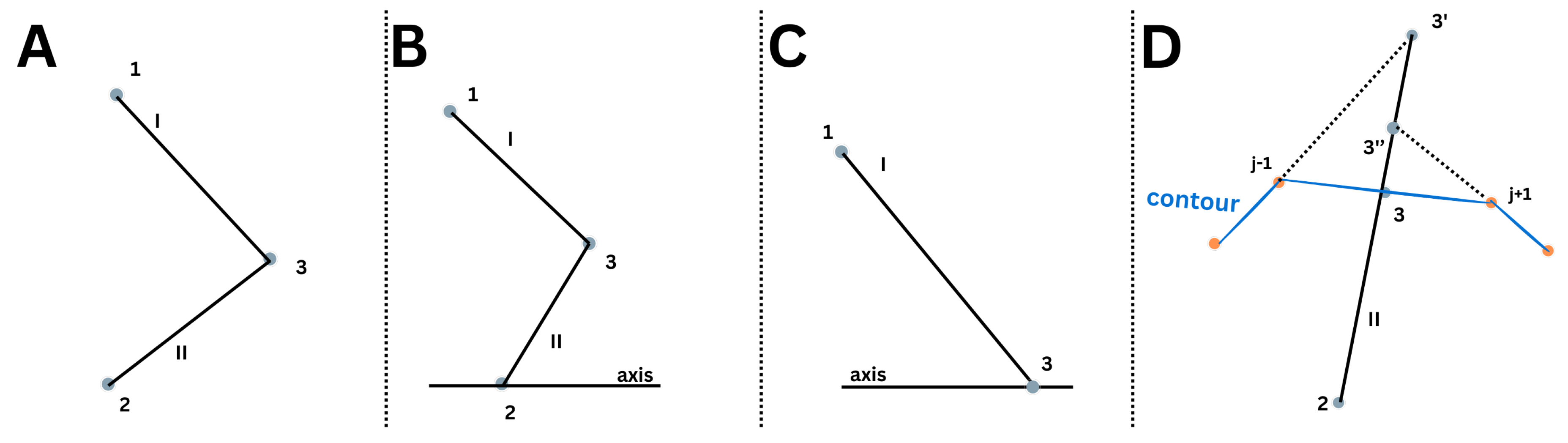
Appendix D. Case A
This represents the generic case, where the point that needs to be calculated is in the interception of two characteristic lines whose properties are known.
In the first iteration, it should be assumed the following:
With algebraic manipulation, Equations A24 to A27 can deliver an estimate of the properties in point 3, present in Equations A30 to A33
With the coefficients given by:
For the next iteration, the properties of each characteristic with be an average between those of the two points on them, such as:
To note the Mach angle for the characteristic is obtained with the Mach number equivalent to the Prandtl-Meyer angle, properly calculated with the method in Appendix ??.
The iterative method should run until the condition of Equation A40 is met.
Appendix E. Case B
If the left characteristic starts on the nozzle axis, meaning point 2 is on the axis with and , leading to Equation A37 being indeterminate on the first iteration.
To prevent so, the indeterminate is solved in the manner of Equation A41.
Applying this philosophy to the method of Case A, for the first iteration of Case B, Equations A32 and A33 are transformed into Equations A42 and A43, respectively.
After the first iteration, the algorithm runs as described for Case A.
Appendix F. Case C
This case represents the interception of a right characteristic line with the axis. Only a characteristic line is necessary to solve the flow as there are only two unknown variables at point 3, as belonging to the axis means and .
Appendix G. Case D
This special case, developed so the in-house algorithms could be repurposed to analyze an already existent contour, arises when a left characteristic is supposed to intercept such already prescribed contour. Supposing the contour is formed by discreet points i, can be given as the spacial derivative given by Equation A46. Between each two discreet points, the contour can be approximated as a straight line, with varying linearly along it.
Utilizing only the iterative averaged Equations for left characteristics, Equation A27 is replaced by finding the point where the characteristic with such slope meets the contour,being the pair of contour points where such interception of straight lines is on their segment . is obtained by the linear approximation leaving to be calculated accordingly with Equation A47.

Table A2.
Variyng number of characteristic lines for and
| Number of Characteristics |
Design Area Ratio |
Theoretical Area Ratio |
Area Ratio Error |
Length | Length Comparison |
|
| 7 | 1.1493 | 1.1484 | 0.08% | 2.289 | 99.99% | |
| 25 | 1.1492 | 1.1484 | 0.07% | 2.289 | 100.00% | |
| 50 | 1.1491 | 1.1484 | 0.06% | 2.289 | 100.00% | |
| 75 | 1.1491 | 1.1484 | 0.06% | 2.289 | 100.00% | |
| 100 | 1.1491 | 1.1484 | 0.06% | 2.289 | 100.00% | |
| 200 | 1.1491 | 1.1484 | 0.05% | 2.289 | 100.00% |
Appendix H. Minimum Length 2D Nozzle Studies
The comparison of the designed minimum length contour for several Mach numbers and adiabatic indexes with 75 characteristics lines can be seen in Table A1.
Table A1.
Several Contours with 75 Characteristics Lines
| Calculated Area Ratio |
Theoretical Area Ratio |
Area Ratio Error |
Length | Length compared to 8º Cone |
||
|---|---|---|---|---|---|---|
| 1.5 | 4/3 | 1.186 | 1.185 | 0.06% | 2.371 | 180.31% |
| 1.5 | 7/5 | 1.177 | 1.176 | 0.06% | 2.352 | 187.62% |
| 1.5 | 5/3 | 1.149 | 1.148 | 0.06% | 2.289 | 216.73% |
| 2.4 | 4/3 | 2.563 | 2.561 | 0.09% | 8.584 | 77.29% |
| 2.4 | 7/5 | 2.405 | 2.403 | 0.08% | 8.093 | 81.06% |
| 2.4 | 5/3 | 2.000 | 1.998 | 0.06% | 6.820 | 96.00% |
| 3 | 4/3 | 4.807 | 4.801 | 0.12% | 19.034 | 70.37% |
| 3 | 7/5 | 4.238 | 4.235 | 0.09% | 16.920 | 73.52% |
| 3 | 5/3 | 3.002 | 3.000 | 0.05% | 12.275 | 86.26% |
| 4.5 | 4/3 | 22.744 | 22.693 | 0.22% | 122.205 | 79.17% |
| 4.5 | 7/5 | 16.583 | 16.562 | 0.12% | 89.971 | 81.25% |
| 4.5 | 5/3 | 7.509 | 7.508 | 0.01% | 42.038 | 90.78% |
Results comparison of the designed contour for pairs of Mach numbers and adiabatic indexes, while varying the number of characteristic lines, can be found in Table A2, Table A3 and Table A4. The pairs of values are (1.5, 5/3), (2.4, 7/5), and (4.5, 4/3) respectively. The last column compares the length of the design with the one under similar conditions but considering 200 characteristic lines, under the assumption that increasing their number improves accuracy.
Appendix I. Minimum Length 2D Nozzle Studies - Varying Specific Heats
Table A5 displays the results from the in-house algorithm that adapts the 2D minimum length bell philosophy with a frozen flow assumption with thermically perfect gas. As for Table A6, it represents the same nozzle contour but with calorically perfect gas. All nozzles use 200 characteristic lines.
Table A3.
Variyng the number of characteristic lines for and
| Number of Characteristics |
Design Area Ratio |
Theoretical Area Ratio |
Area Ratio Error |
Length | Length Comparison |
|
| 7 | 2.4047 | 2.4031 | 0.07% | 8.089 | 99.96% | |
| 25 | 2.4053 | 2.4031 | 0.09% | 8.093 | 100.02% | |
| 50 | 2.4051 | 2.4031 | 0.08% | 8.093 | 100.01% | |
| 75 | 2.4049 | 2.4031 | 0.08% | 8.093 | 100.01% | |
| 100 | 2.4048 | 2.4031 | 0.07% | 8.092 | 100.00% | |
| 200 | 2.4047 | 2.4031 | 0.07% | 8.092 | 100.00% |
Table A4.
Variyng the number of characteristic lines for and
| Number of Characteristics |
Design Area Ratio |
Theoretical Area Ratio |
Area Ratio Error |
Length | Length Comparison |
|
| 7 | 24.2685 | 22.6933 | 6.94% | 129.222 | 105.79% | |
| 25 | 22.8236 | 22.6933 | 0.57% | 122.573 | 100.34% | |
| 50 | 22.7566 | 22.6933 | 0.28% | 122.265 | 100.09% | |
| 75 | 22.7435 | 22.6933 | 0.22% | 122.205 | 100.04% | |
| 100 | 22.7385 | 22.6933 | 0.20% | 122.181 | 100.02% | |
| 200 | 22.7324 | 22.6933 | 0.17% | 122.152 | 100.00% |
Table A5.
Contour for Thermically Perfect Gas of Minimum Length 2D Nozzle
| Stagnation Temperature (K) |
Design |
(º) |
Length |
Measured |
|||
| 500 | 1.5 | 5.959 | 2.352 | 1.177 | 1.398 | 1.500 | |
| 2.4 | 18.374 | 8.090 | 2.404 | 1.400 | 2.400 | ||
| 4.5 | 35.916 | 89.916 | 16.572 | 1.400 | 4.499 | ||
| 1000 | 1.5 | 6.094 | 2.361 | 1.181 | 1.363 | 1.500 | |
| 2.4 | 18.544 | 8.110 | 2.414 | 1.390 | 2.400 | ||
| 4.5 | 35.916 | 88.835 | 16.374 | 1.400 | 4.499 | ||
| 1500 | 1.5 | 6.228 | 2.352 | 1.186 | 1.329 | 1.500 | |
| 2.4 | 19.084 | 8.308 | 2.480 | 1.360 | 2.401 | ||
| 4.5 | 35.943 | 85.929 | 15.859 | 1.399 | 4.499 | ||
| 3000 | 1.5 | 6.356 | 2.372 | 1.190 | 1.298 | 1.500 | |
| 2.4 | 19.084 | 8.767 | 2.624 | 1.309 | 2.401 | ||
| 4.5 | 35.943 | 89.877 | 16.674 | 1.372 | 4.500 | ||
| 5000 | 1.5 | 6.388 | 2.385 | 1.192 | 1.290 | 1.500 | |
| 2.4 | 20.372 | 8.915 | 2.671 | 1.294 | 2.401 | ||
| 4.5 | 39.860 | 119.581 | 22.309 | 1.325 | 4.502 |
Table A6.
Contour for Calorically Perfect Gas of Minimum Length 2D Nozzle
|
Design |
(º) |
Length |
Measured |
||
|---|---|---|---|---|---|
| 1.5 | 5.953 | 2.352 | 1.177 | 1.4 | 1.500 |
| 2.4 | 18.373 | 8.092 | 2.405 | 1.4 | 2.400 |
| 4.5 | 35.916 | 89.939 | 16.576 | 1.4 | 4.499 |
Appendix J. Minimum Length 2D Nozzle Studies -Boundary Layer Correction
Table A7 presents the results obtained from two in-house algorithms. One assumes a calorically perfect gas, while the other employs a frozen flow assumption with thermically perfect gas, both simulating a boundary layer around the inviscid contour and displacing it accordingly. The stagnation temperature of the flow varies in these simulations. In Table A8, similar exercises were conducted with variations in stagnation pressure. All nozzles in these analyses were designed using 200 characteristic lines.
Table A7.
Boundary-Layer Displacement Thickness at the Exit of the Inviscid Nozzle v.s. Stagnation Temperature
Table A7.
Boundary-Layer Displacement Thickness at the Exit of the Inviscid Nozzle v.s. Stagnation Temperature
| Stagnation Temperature (K) |
Design |
as Percentage of Throat Radius at the Exit Lip |
||
| Calorically Perfect |
Thermically Perfect |
|||
| 500 | 1.5 | 0.393% | 0.398% | |
| 2.4 | 1.293% | 1.404% | ||
| 4.5 | 12.857% | 16.387% | ||
| 1000 | 1.5 | 0.457% | 0.465% | |
| 2.4 | 1.492% | 1.593% | ||
| 4.5 | 14.818% | 18.888% | ||
| 1500 | 1.5 | 0.500% | 0.512% | |
| 2.4 | 1.639% | 1.797% | ||
| 4.5 | 15.983% | 20.383% | ||
| 3000 | 1.5 | 0.580% | 0.596% | |
| 2.4 | 1.908% | 2.138% | ||
| 4.5 | 19.119% | 24.772% | ||
| 5000 | 1.5 | 0.645% | 0.664% | |
| 2.4 | 2.126% | 2.395% | ||
| 4.5 | 21.444% | 29.577% | ||
Appendix K. Minimum Length Axisymmetric Nozzle Studies
The comparison of the resulting designed contour for several Mach numbers and adiabatic indexes with an also varying number of characteristics lines can be seen in Table A9.
Table A9.
Several Studies for Several Mach numbers and
| Number of lines |
Obtained Radius Ratio |
Theoretical Radius Ratio |
Radius Ratio Error |
Length | Length compared to 8º Cone |
(°) |
Obtained |
|||
| 1.5 | 4/3 | 184 | 1.073 | 1.088 | -1.47% | 2.021 | 321% | 2.59 | 1.501 | |
| 1.5 | 7/5 | 184 | 1.069 | 1.085 | -1.40% | 2.104 | 335% | 2.49 | 1.501 | |
| 1.5 | 5/3 | 183 | 1.059 | 1.072 | -1.22% | 1.986 | 390% | 2.13 | 1.502 | |
| 2.4 | 4/3 | 274 | 1.536 | 1.600 | -3.99% | 5.192 | 122% | 8.98 | 2.400 | |
| 2.4 | 7/5 | 273 | 1.491 | 1.550 | -3.81% | 5.041 | 129% | 8.40 | 2.402 | |
| 2.4 | 5/3 | 269 | 1.366 | 1.414 | -3.39% | 4.611 | 157% | 6.68 | 2.402 | |
| 3 | 4/3 | 309 | 2.091 | 2.191 | -4.58% | 8.614 | 102% | 12.77 | 3.001 | |
| 3 | 7/5 | 308 | 1.972 | 2.058 | -4.19% | 8.156 | 108% | 11.82 | 3.007 | |
| 3 | 5/3 | 302 | 1.665 | 1.732 | -3.92% | 6.917 | 133% | 9.08 | 3.005 | |
| 4.5 | 4/3 | 327 | 4.558 | 4.764 | -4.32% | 25.969 | 97% | 19.80 | 4.505 | |
| 4.5 | 7/5 | 325 | 3.898 | 4.070 | -4.23% | 22.375 | 102% | 17.94 | 4.511 | |
| 4.5 | 5/3 | 317 | 2.620 | 2.740 | -4.39% | 15.292 | 124% | 13.12 | 4.506 |
Results comparison of the designed contour for pairs of Mach numbers and adiabatic indexes, while varying the number of characteristic lines, can be found in Table A10, Table A11 and Table A12. The pairs of values are (1.5, 5/3), (2.4, 7/5), and (4.5, 4/3) respectively. These tables confirm the assumption that increasing the number of characteristics improves accuracy.
Table A10.
Several Contours for Various Design Conditions for M=1.5 and
| Number of Characteristics |
Obtained } |
Area Ratio |
Area Ratio Error |
Length |
(°) |
|
| 7 | 1.520 | 1.069 | -0.25% | 2.044 | 2.25 | |
| 21 | 1.505 | 1.061 | -0.98% | 1.997 | 2.15 | |
| 50 | 1.508 | 1.060 | -1.04% | 2.002 | 2.16 | |
| 62 | 1.506 | 1.060 | -1.10% | 1.996 | 2.15 | |
| 183 | 1.502 | 1.059 | -1.22% | 1.986 | 2.13 |
Table A8.
Boundary-Layer Displacement Thickness at the Exit of the Inviscid Nozzle v.s. Stagnation Pressure
Table A8.
Boundary-Layer Displacement Thickness at the Exit of the Inviscid Nozzle v.s. Stagnation Pressure
| Stagnation Pressure (MPa) |
Design |
as Percentage of Throat Radius at the Exit Lip |
||
| Calorically Perfect |
Thermically Perfect |
|||
| 0.5 | 1.5 | 0.574% | 0.588% | |
| 2.4 | 1.882% | 2.065% | ||
| 4.5 | 18.584% | 23.307% | ||
| 1 | 1.5 | 0.500% | 0.512% | |
| 2.4 | 1.639% | 1.797% | ||
| 4.5 | 15.983% | 20.383% | ||
| 2 | 1.5 | 0.435% | 0.445% | |
| 2.4 | 1.417% | 1.557% | ||
| 4.5 | 14.477% | 18.461% | ||
Table A11.
Varying number of characteristic lines for and
| Number of Characteristics |
Obtained |
Area Ratio |
Area Ratio Error |
Length |
(°) |
|---|---|---|---|---|---|
| 7 | 2.532 | 1.678 | 8.23% | 5.849 | 9.24 |
| 24 | 2.446 | 1.547 | -0.23% | 5.291 | 8.68 |
| 46 | 2.403 | 1.503 | -3.03% | 5.070 | 8.41 |
| 65 | 2.420 | 1.511 | -2.51% | 5.138 | 8.51 |
| 83 | 2.413 | 1.504 | -2.95% | 5.104 | 8.47 |
| 137 | 2.404 | 1.495 | -3.56% | 5.056 | 8.41 |
| 273 | 2.402 | 1.491 | -3.81% | 5.041 | 8.40 |
Table A12.
Varying number of characteristic lines for and
| Number of Characteristics |
Obtained |
Area Ratio |
Area Ratio Error |
Length |
(°) |
|---|---|---|---|---|---|
| 8 | 4.506 | 5.594 | 17.44% | 20.465 | 19.72 |
| 25 | 4.603 | 5.174 | 8.62% | 29.448 | 20.14 |
| 51 | 4.542 | 4.801 | 0.78 % | 27.299 | 19.92 |
| 101 | 5.514 | 4.643 | -2.54 % | 26.392 | 19.82 |
| 137 | 4.505 | 4.591 | -3.62% | 26.100 | 19.79 |
| 327 | 4.512 | 4.574 | -3.99% | 26.073 | 19.81 |
Appendix L. Parabola Nozzle Performance MOC Studies
Figure A2 shows the typical net of characteristics and nodes used to evaluate the parabolic nozzle performance at the design point.
Figure A2.
Parabolic Bell Nozzle for , , , and of a 15º conical nozzle
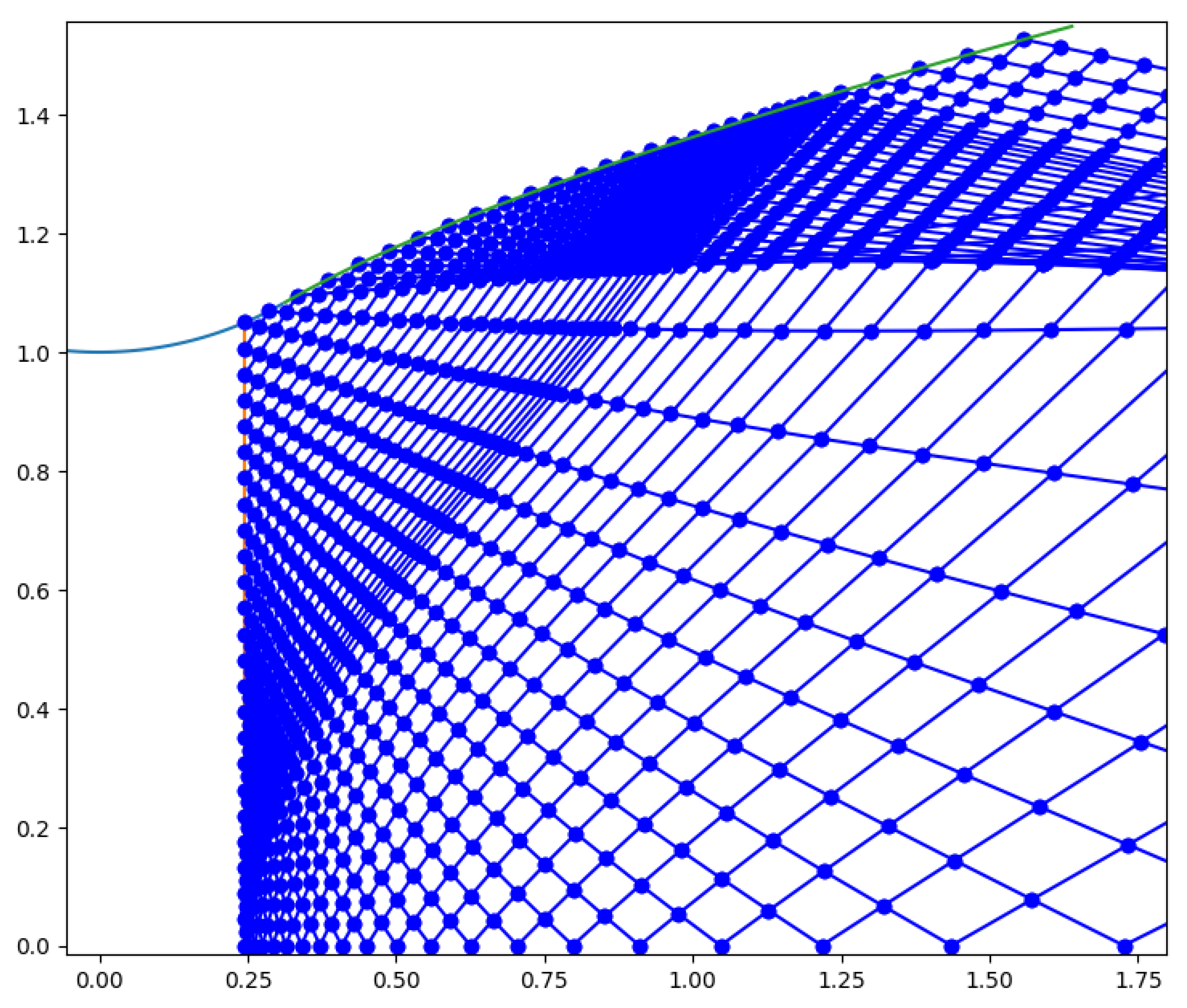
Table A13.
Specific Impulse from In-house Algorithm vs number of nodes of the initial line
| Number of Nodes in Initial Line |
(s) |
of Quasi-1D Conical Nozzle |
(º) |
|||
|---|---|---|---|---|---|---|
| 25 | 594.268 | 98.62% | 2.209 | 2.584 | 2.395 | 18.148 |
| 50 | 591.392 | 98.14% | 2.200 | 2.572 | 2.396 | 18.165 |
| 100 | 591.181 | 98.11% | 2.199 | 2.507 | 2.397 | 18.172 |
| 150 | 590.742 | 98.03% | 2.199 | 2.491 | 2.396 | 18.165 |
| 200 | 590.934 | 98.07% | 2.198 | 2.480 | 2.396 | 18.161 |
| 300 | 590.923 | 98.06% | 2.198 | 2.470 | 2.397 | 18.169 |
Table A14.
Specific Impulse from In-house Algorithm vs design Mach number
| Design |
(s) |
of Quasi-1D Conical Nozzle |
(º) |
|||
|---|---|---|---|---|---|---|
| 2 | 525.035 | 95.62% | 1.909 | 2.092 | 2.105 | 20.715 |
| 2.4 | 590.934 | 98.07% | 2.198 | 2.480 | 2.396 | 18.161 |
| 3 | 659.752 | 99.91% | 2.770 | 3.299 | 3.123 | 14.137 |
| 4 | 725.353 | 100.90% | 3.857 | 4.808 | 4.519 | 7.900 |
Table A15.
Specific Impulse from In-house Algorithm vs circle arc angle
|
(º) |
(s) |
of Quasi-1D Conical Nozzle |
(º) |
|||
|---|---|---|---|---|---|---|
| 25 | 591.460 | 98.15% | 2.199 | 2.480 | 2.404 | 18.498 |
| 30 | 590.934 | 98.07% | 2.198 | 2.480 | 2.396 | 18.161 |
| 35 | 591.106 | 98.09% | 2.196 | 2.480 | 2.386 | 17.802 |
| 40 | 592.111 | 98.26% | 2.195 | 2.480 | 2.362 | 17.092 |
| 45 | 595.827 | 98.88% | 2.191 | 2.480 | 2.325 | 16.048 |
| 50 | 601.379 | 99.80% | 2.204 | 2.480 | 2.301 | 14.190 |
Table A16.
Specific Impulse from In-house Algorithm vs exit divergence angle and comparable cone half angle
Table A16.
Specific Impulse from In-house Algorithm vs exit divergence angle and comparable cone half angle
| Exit Divergence (º) |
(s) |
of Quasi-1D Conical Nozzle |
(º) |
|||
|---|---|---|---|---|---|---|
| 15 | 590.934 | 98.07% | 2.198 | 2.480 | 2.396 | 18.161 |
| 12 | 610.230 | 100.01% | 2.211 | 2.717 | 2.407 | 11.275 |
| 10 | 616.959 | 100.42% | 2.265 | 2.594 | 2.486 | 4.767 |
Table A17.
Specific Impulse from In-house Algorithm vs conical nozzle length fraction f
| f |
(s) |
of Quasi-1D Conical Nozzle |
(º) |
|||
|---|---|---|---|---|---|---|
| 0.6 | 550.852 | 91.41% | 2.091 | 2.259 | 2.550 | 27.063 |
| 0.7 | 574.428 | 95.33% | 2.139 | 2.368 | 2.440 | 22.032 |
| 0.8 | 590.934 | 98.07% | 2.198 | 2.480 | 2.396 | 18.161 |
| 0.9 | 604.035 | 100.24% | 2.262 | 2.572 | 2.377 | 14.470 |
| 1 | 610.309 | 101.28% | 2.328 | 2.468 | 2.384 | 10.406 |
Table A18.
Specific Impulse from In-house Algorithm vs chamber stagnation temperature
| Stagnation Temperature (K) |
(s) |
of Quasi-1D Conical Nozzle |
(º) |
|||
|---|---|---|---|---|---|---|
| 750 | 467.175 | 98.07% | 2.198 | 2.480 | 2.396 | 18.161 |
| 1200 | 590.934 | 98.07% | 2.198 | 2.480 | 2.396 | 18.161 |
| 2000 | 762.893 | 98.07% | 2.198 | 2.480 | 2.396 | 18.161 |
Table A19.
Specific Impulse from In-house Algorithm vs chamber stagnation pressure
| Stagnation Pressure (MPa) |
(s) |
of Quasi-1D Conical Nozzle |
(º) |
|||
|---|---|---|---|---|---|---|
| 0.5 | 590.934 | 98.07% | 2.198 | 2.480 | 2.396 | 18.161 |
| 1 | 590.934 | 98.07% | 2.198 | 2.480 | 2.396 | 18.161 |
| 2 | 590.934 | 98.07% | 2.198 | 2.480 | 2.396 | 18.161 |
List of Acronyms
| AUSM | Advection Upstream Splitting Method |
| CAD | Computer-Aided Design |
| CFD | Computational Fluid Dynamics |
| CTIC | Compressed Truncated Ideal Contoured |
| EUPO | Estágio Único Para Órbita |
| FSS | Free Shock Separation |
| ISRU | In Situ Resource Utilization |
| MN | Mach Number |
| MNG | Multi Nozzle Grids |
| MOC | Method of Characteristics |
| ODE | Ordinary Differential Equation |
| PDE | Partial Differential Equation |
| PR | Pressure Ratio |
| RANS | Reynolds Average Navier-Strokes |
| Roe-FDS | Roe Flux-Difference Splitting |
| RNG | Renormalization Group (Theory) |
| RSS | Restricted Shock Separation |
| SSTO | Single-stage-to-orbit vehicles |
| TIC | Truncated Idealized Contoured |
| TOC | Thrust Optimized Contoured |
References
- A. F. El-Sayed, “Rocket propulsion,” in Fundamentals of Aircraft and Rocket Propulsion, pp. 907–991, Springer London, May 2016. [CrossRef]
- S. Khare and U. K. Saha, “Rocket nozzles: 75 years of research and development,” Sādhanā, vol. 46, Apr. 2021. [CrossRef]
- G. Sutton and O. Biblarz, Rocket Propulsion Elements. A Wiley Interscience publication, Wiley, 2001. ISBN: 9780471326427.
- A. A. Hussaini, “Chapter Eleven/Normal shock in converging–diverging nozzles ,” Sept. 2013. [Online]. Available: https://cnj.atu.edu.iq/wp-content/uploads/2019/09/Gas-Dynamic-3.pdf.
- A. A. Hussaini, “Chapter Sixteen / Plug, Underexpanded and Overexpanded Supersonic Nozzles,” Sept. 2013. [Online]. Available: https://cnj.atu.edu.iq/wp-content/uploads/2020/03/Gas-Dynamic-4.pdf.
- J. Anderson, Modern Compressible Flow, with Historical Perspective. McGraw-Hill series in Aeronautical and Aerospace Engineering, McGraw-Hill, 1982. ISBN: 9780070016545.
- I. M. Hall, “Inversion of the prandtl-meyer relation,” The Aeronautical Journal, vol. 79, p. 417–418, Sept. 1975. [CrossRef]
- I. M. HALL, “Transonic flow in two-dimensional and axially-symmetric nozzles,” The Quarterly Journal of Mechanics and Applied Mathematics, vol. 15, no. 4, p. 487–508, 1962. [CrossRef]
- J. R. KLIEGEL and J. N. LEVINE, “Transonic flow in small throat radius of curvature nozzles.,” AIAA Journal, vol. 7, p. 1375–1378, July 1969. [CrossRef]
- J. C. Dutton and A. L. Addy, “Transonic flow in the throat region of axisymmetric nozzles,” AIAA Journal, vol. 19, p. 801–804, June 1981. [CrossRef]
- Ansys, “Method of Characteristics - Internal Compressible Flows – Lesson 6,” Nov. 2020. [Online]. Available: https://courses.ansys.com/index.php/courses/internal-compressible-flows/lesson s/method-of-characteristics-lesson-6/.
- T. Zebbiche, “Stagnation pressure effect on the supersonic minimum length nozzle design,” The Aeronautical Journal, vol. 123, p. 1013–1031, June 2019. [CrossRef]
- J. C. Restrepo, A. F. Bolaños-Acosta, and J. R. Simões-Moreira, “Short nozzles design for real gas supersonic flow using the method of characteristics,” Applied Thermal Engineering, vol. 207, p. 118063, May 2022. [CrossRef]
- M. Reedy, “The Most Popular Coding Languages Used In Aerospace,” Dec. 2021.
- B. Li, J. Wu, and Y. Liu, “Numerical study on subsonic-supersonic laval nozzle using maccormack scheme,” Journal of Physics: Conference Series, vol. 2012, p. 012096, Sept. 2021. [CrossRef]
- MIT, “Basics of Turbulent Flow.”.
- L. Davidson, “An Introduction to Turbulence Models,” Aug. 2022. [Online]. Available: https://www.tfd.chalmers.se/ lada/postscript_files/kompendium_turb.pdf.
- Ansys, “Ansys Fluent Theory Guide,” July 2021.
- J. Kola and V. Dvo, “Verification of kω sst turbulence model for supersonic internal flows,” 2013.
- T. Benson, “Specific Heat Capacity - Calorically Imperfect Gas,” May 2021.
- M. Matsunaga, C. Fujio, H. Ogawa, Y. Higa, and T. Handa, “Nozzle design optimization for supersonic wind tunnel by using surrogate-assisted evolutionary algorithms,” Aerospace Science and Technology, vol. 130, p. 107879, Nov. 2022. [CrossRef]
- F. P. BOYNTON, “Exhaust plumes from nozzles with wall boundary layers.,” Journal of Spacecraft and Rockets, vol. 5, p. 1143–1147, Oct. 1968. [CrossRef]
- Y. WANG and Z. JIANG, “Theories and methods for designing hypersonic high-enthalpy flow nozzles,” Chinese Journal of Aeronautics, vol. 35, p. 318–339, Jan. 2022. [CrossRef]
- C. Documentation, “Sutherland’s Law.”.
- F. Ding, J. Liu, W. Huang, Y. Zhou, and S. Guo, “Boundary-layer viscous correction method for hypersonic forebody/inlet integration,” Acta Astronautica, vol. 189, p. 638–657, Dec. 2021.
- A. EDWARDS and J. PERKINS, “Limitations of the method of characteristics when applied to axisymmetric hypersonic nozzle design,” in 28th Aerospace Sciences Meeting, American Institute of Aeronautics and Astronautics, Jan. 1990. [CrossRef]
- T. Fernandes, A. Souza, and F. Afonso, “A shape design optimization methodology based on the method of characteristics for rocket nozzles,” CEAS Space Journal, July 2023. [CrossRef]
- J. Östlund and B. Muhammad-Klingmann, “Supersonic flow separation with application to rocket engine nozzles,” Applied Mechanics Reviews, vol. 58, pp. 143–177, May 2005. [CrossRef]
- D. Munday, E. Gutmark, J. Liu, and K. Kailasanath, “Flow structure and acoustics of supersonic jets from conical convergent-divergent nozzles,” Physics of Fluids, vol. 23, Nov. 2011. [CrossRef]
- R. Jia, Z. Jiang, and W. Zhang, “Numerical analysis of flow separation and side loads of a conical nozzle during staging,” Proceedings of the Institution of Mechanical Engineers, Part G: Journal of Aerospace Engineering, vol. 230, p. 845–855, Aug. 2015. [CrossRef]
- H. M. DAKWELL and H. BADHAM, “Shock formation in conical nozzles,” AIAA Journal, vol. 1, p. 1932–1934, Aug. 1963. [CrossRef]
- N. K. Mishra, A. Kumar, M. Ganesh, and M. A. R. Alam, “Design of minimum length supersonic nozzle using the method of characteristics,” International Journal of Innovative Technology and Exploring Engineering, vol. 9, pp. 1370–1374, Dec. 2019. [CrossRef]
- D. Sun, T. Luo, and Q. Feng, “New contour design method for rocket nozzle of large area ratio,” International Journal of Aerospace Engineering, vol. 2019, p. 1–8, Dec. 2019. [CrossRef]
- G. V. R. RAO, “Exhaust nozzle contour for optimum thrust,” Journal of Jet Propulsion, vol. 28, pp. 377–382, June 1958. [CrossRef]
- Rick Newlands, “The Thrust Optimised Parabolic nozzle,” Apr. 2017. [Online]. Available: https://www.aspirespace.org.uk/downloads/Thrust%20optimised%20 parabolic%20nozzle.pdf.
- C. Lee, K. Choi, C. Kim, and S. Han, “Computational investigation of flow separation in a thrust-optimized parabolic nozzle during high-altitude testing,” Computers and Fluids, vol. 197, p. 104363, Jan. 2020. [CrossRef]
- S. B. Verma and O. Haidn, “Study of restricted shock separation phenomena in a thrust optimized parabolic nozzle,” Journal of Propulsion and Power, vol. 25, p. 1046–1057, Sept. 2009. [CrossRef]
- M. Takahashi, S. Ueda, T. Tomita, M. Takahashi, H. Tamura, and K. Aoki, “Transient flow simulation of a compressed truncated perfect nozzle,” in 37th Joint Propulsion Conference and Exhibit, American Institute of Aeronautics and Astronautics, July 2001. [CrossRef]
- R. Stark and B. Wagner, “Experimental flow investigation of a truncated ideal contour nozzle,” in 42nd AIAA/ASME/SAE/ASEE Joint Propulsion Conference and Exhibit, American Institute of Aeronautics and Astronautics, July 2006. [CrossRef]
- F. Bakulu, G. Lehnasch, V. Jaunet, E. Goncalves da Silva, and S. Girard, “Jet resonance in truncated ideally contoured nozzles,” Journal of Fluid Mechanics, vol. 919, May 2021. [CrossRef]
- J. D. Hoffman, “Design of compressed truncated perfect nozzles,” Journal of Propulsion and Power, vol. 3, p. 150–156, Mar. 1987. [CrossRef]
- J. L. POTTER and W. H. CARDEN, “Design of axisymmetric contoured nozzles for laminar hypersonic flow.,” Journal of Spacecraft and Rockets, vol. 5, p. 1095–1100, Sept. 1968. [CrossRef]
- James R. Betnton, “Design and Navier-Stokes analysis of hypersonic wind tunnel nozzles,” Jan. 1989. [Online]. Available: https://ntrs.nasa.gov/citations/19890019982.
- R. L. Gaffney, “Design of a pulse-facility nozzle using the rotational method of characteristics,” Journal of Spacecraft and Rockets, vol. 43, p. 1216–1224, Nov. 2006. [CrossRef]
- K. FOELSCH, “The analytical design of an axially symmetric laval nozzle for a parallel and uniform jet,” Journal of the Aeronautical Sciences, vol. 16, p. 161–166, Mar. 1949. [CrossRef]
- J. C. SIVELLS, “Aerodynamic design of axisymmetric hypersonic wind-tunnel nozzles,” Journal of Spacecraft and Rockets, vol. 7, p. 1292–1299, Nov. 1970. [CrossRef]
- J. C. Sivells, “A Computer Program for the Aerodynamic Design of Axisymmetric and Planar Nozzles for Supersonic and Hypersonic Wind Tunnels,” Dec. 1978. [Online]. Available: https://apps.dtic.mil/sti/citations/ADA062944.
- Noah Stockwell, “ConturPy: Python Hypersonic Nozzle Design,” Apr. 2022. [Online]. Available: https://github.com/noahess/conturpy.
- G. Hagemann, H. Immich, T. Van Nguyen, and G. E. Dumnov, “Advanced rocket nozzles,” Journal of Propulsion and Power, vol. 14, p. 620–634, Sept. 1998. [CrossRef]
- S. Corda, Flight Testing the Linear Aerospike SR-71 Experiment (LASRE). NASA technical memorandum, NASA Dryden Flight Research Center, 1998. [ONLINE]. Available: https://books.google.pt/books?id=mbM3AQAAMAAJ.
- P. P. Nair, A. Suryan, and H. D. Kim, “Computational study of performance characteristics for truncated conical aerospike nozzles,” Journal of Thermal Science, vol. 26, pp. 483–489, Nov. 2017. [CrossRef]
- J. Scott, “Aerospike Aerodynamics,” Oct. 1999.
- N. Erni, C. Frazier, and D. Baker, “Attitude control using aerodynamic vectoring on an aerospike nozzle,” Nov. 2011.
- H. Greer, “Rapid method for plug nozzle design,” ARS Journal, vol. 31, pp. 560–561, Apr. 1961.
- G. Angelino, “Approximate method for plug nozzle design,” AIAA Journal, vol. 2, pp. 1834–1835, Oct. 1964. [CrossRef]
- C.-H. Wang, Y. Liu, and L.-Z. Qin, “Aerospike nozzle contour design and its performance validation,” Acta Astronautica, vol. 64, pp. 1264–1275, June 2009. [CrossRef]
- K. N. Kumar, M. Gopalsamy, D. Antony, R. Krishnaraj, and C. B. V. Viswanadh, “Design and optimization of aerospike nozzle using CFD,” IOP Conference Series: Materials Science and Engineering, vol. 247, p. 012008, Oct. 2017. [CrossRef]
- S. Dakka and O. Dennison, “Numerical analysis of aerospike engine nozzle performance at various truncation lengths,” International Journal of Aviation, Aeronautics, and Aerospace, June 2021. [CrossRef]
- A. Padania, S. K. Sardiwal, D. H. Chowdary, M. S. Sharath, and S. Artham, “Numerical solution for the design of a traditional aerospike nozzle using method of characteristics,” IOSR Journal of Mechanical and Civil Engineering (IOSR-JMCE), Feb. 2015. [Online]. Available: https://www.iosrjournals.org/iosr-jmce/papers/vol12-issue1/Version-4/L0121463 69.pdf.
- S. Khan, A. Khan, and A. Munir, “Design and analysis approach for linear aerospike nozzle,” Science Vision, vol. 20, pp. 25 – 37, 07 2014.
- H. F. R. Schoyer, “Thrust vector control for (clustered modules) plug nozzles: Some considerations,” Journal of Propulsion and Power, vol. 16, pp. 196–201, Mar. 2000. [CrossRef]
- C. Bach, J. Sieder-Katzmann, M. Propst, and M. Tajmar, “Evaluation of the performance potential of aerodynamically thrust vectored aerospike nozzles,” Sept. 2016.
- T. Mizukaki and S. Watabe, “Visualization of stagnation point inside the closed wake of a 20%-truncated plug nozzle at starting process,” Aerospace Science and Technology, vol. 50, pp. 25–30, Mar. 2016. [CrossRef]
- C. Aukerman, “Plug nozzles - The ultimate customer driven propulsion system,” in 27th Joint Propulsion Conference, American Institute of Aeronautics and Astronautics, June 1991. [CrossRef]
- A. Lai, S. S. Wei, C. H. Lai, J. L. Chen, Y. H. Liao, J. S. Wu, and Y. S. Chen, “Comparison of the propulsion performance of aerospike and bell-shaped nozzle using hydrogen peroxide monopropellant under sea-level condition,” Journal of Mechanics, vol. 35, pp. 427–440, July 2018. [CrossRef]
- T. Ito and K. Fujii, “Numerical analysis of the base bleed effect on the aerospike nozzles,” in 40th AIAA Aerospace Sciences Meeting Exhibit, American Institute of Aeronautics and Astronautics, Jan. 2002. [CrossRef]
- G. Hagemann, H. Immich, and M. Terhardt, “Flow phenomena in advanced rocket nozzles - the plug nozzle,” in 34th AIAA/ASME/SAE/ASEE Joint Propulsion Conference and Exhibit, American Institute of Aeronautics and Astronautics, July 1998. [CrossRef]
- N. Taylor, J. Steelant, and R. Bond, “Experimental comparison of dual bell and expansion deflection nozzles,” in 47th AIAA/ASME/SAE/ASEE Joint Propulsion Conference Exhibit, American Institute of Aeronautics and Astronautics, July 2011. [CrossRef]
- M. C. Karia, M. A. Popat, and K. B. Sangani, “Selective laser melting of Inconel super alloy-a review,” in AIP Conference Proceedings, July 2017. [CrossRef]
- F. B. Cowles and C. R. Foster, “Experimental study of gas-flow separation in overexpanded exhaust nozzles for rocket motors,” 1949. [Online]. Available: https://api.semanticscholar.org/CorpusID:135861885.
- H. Immich, M. Caporicci, H. Immich, and M. Caporicci, “Status of the festip rocket propulsion technology programme,” in 33rd Joint Propulsion Conference and Exhibit, American Institute of Aeronautics and Astronautics, July 1997. [CrossRef]
- A. Ferrero, A. Conte, E. Martelli, F. Nasuti, and D. Pastrone, “Dual-bell nozzle with fluidic control of transition for space launchers,” Acta Astronautica, vol. 193, p. 130–137, Apr. 2022. [CrossRef]
- N. Taylor, J. Steelant, and R. Bond, “Experimental comparison of dual bell and expansion deflection nozzles,” in 47th AIAA/ASME/SAE/ASEE Joint Propulsion Conference Exhibit, American Institute of Aeronautics and Astronautics, July 2011. [CrossRef]
- M. Frey and G. Hagemann, “Critical assessment of dual-bell nozzles,” Journal of Propulsion and Power, vol. 15, p. 137–143, Jan. 1999. [CrossRef]
- Y. Wang, Y. Lin, Q. Eri, and B. Kong, “Flow and thrust characteristics of an expansion–deflection dual-bell nozzle,” Aerospace Science and Technology, vol. 123, p. 107464, Apr. 2022. [CrossRef]
- H. Kbab, M. Sellam, T. Hamitouche, S. Bergheul, and L. Lagab, “Design and performance evaluation of a dual bell nozzle,” Acta Astronautica, vol. 130, p. 52–59, Jan. 2017. [CrossRef]
- H. Kbab†, O. Abada, and S. Haif, “Numerical investigation of supersonic flows on innovative nozzles (dual bell nozzle),” Journal of Applied Fluid Mechanics, vol. 16, Apr. 2023. [CrossRef]
- K. Wu, G. C. Sohn, R. Deng, H. Jia, H. D. Kim, and X. Su, “Study on wall pressure and hysteresis behaviors of a novel dual-bell nozzle,” Journal of Mechanical Science and Technology, vol. 37, p. 4639–4646, Sept. 2023. [CrossRef]
- H. Otsu, M. Miyazawa, and Y. Nagata, “Design criterion of the dual-bell nozzle contour,” in 56th International Astronautical Congress of the International Astronautical Federation, the International Academy of Astronautics, and the International Institute of Space Law, American Institute of Aeronautics and Astronautics, Oct. 2005. [CrossRef]
- M. Miyazawa, S. Takeuchi, and M. Takahashi, “Flight performance of dual-bell nozzles,” in 40th AIAA Aerospace Sciences Meeting and Exhibit, American Institute of Aeronautics and Astronautics, Jan. 2002. [CrossRef]
- G. V. R. RAO, Liquid Rockets And Propellants. American Institute of Aeronautics and Astronautics, Jan. 1960. [CrossRef]
- N. V. Taylor and C. M. Hempsell, “Optimising expansion deflection nozzles for vacuum thrust,” The Aeronautical Journal, vol. 108, p. 515–522, Oct. 2004. [CrossRef]
- K. Schomberg, G. Doig, and J. Olsen, “Computational simulation of an altitude adaptive nozzle concept,” Applied Mechanics and Materials, vol. 553, p. 223–228, May 2014. [CrossRef]
- J. Paul P., P. P. Nair, A. Suryan, J. P. Martin M, and H. Dong Kim, “Numerical simulation on optimization of pintle base shape in planar expansion-deflection nozzles,” Journal of Spacecraft and Rockets, vol. 57, p. 539–548, May 2020. [CrossRef]
- D. Chasman, M. Birch, S. Haight, and R. Graffam, “A multi-disciplinary optimization method for multi nozzle grid (MNG) design - final report,” in 43rd AIAA Aerospace Sciences Meeting and Exhibit, American Institute of Aeronautics and Astronautics, Jan. 2005. [CrossRef]
- R. H. Schmucker, “Flow processes in overexpanded chemical rocket nozzles. Part 1: Flow separation,” in NASA Technical Reports Server, Technische Univ. Munich, Germany, July 1973. [Online]. Available: https://ntrs.nasa.gov/citations/19750017939.
- N. Goncharov, V. Orlov, V. Rachuk, A. Shostak, and R. Starke, “Reusable launch vehicle propulsion based on the RD-0120 engine,” in 31st Joint Propulsion Conference and Exhibit, American Institute of Aeronautics and Astronautics, July 1995. [CrossRef]
- G. V. R. RAO, “Exhaust nozzle contour for optimum thrust,” Journal of Jet Propulsion, vol. 28, pp. 377–382, June 1958. [CrossRef]
- J. C. Silva and F. Brójo, “Aerospike nozzle contour design using angelino’s method and cfd validation,” Discover Mechanical Engineering, vol. 3, Oct. 2024.
Figure 1.
Velocity, Temperature and Pressure variations along a de Laval Nozzle [2]
Figure 1.
Velocity, Temperature and Pressure variations along a de Laval Nozzle [2]
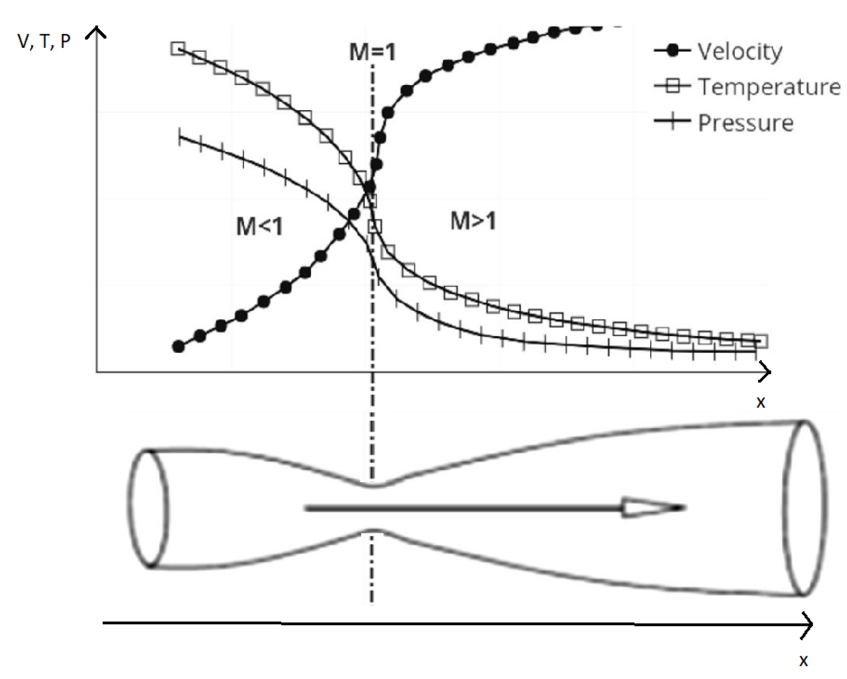
Figure 2.
Nozzle’s modes of operation [4]
Figure 2.
Nozzle’s modes of operation [4]
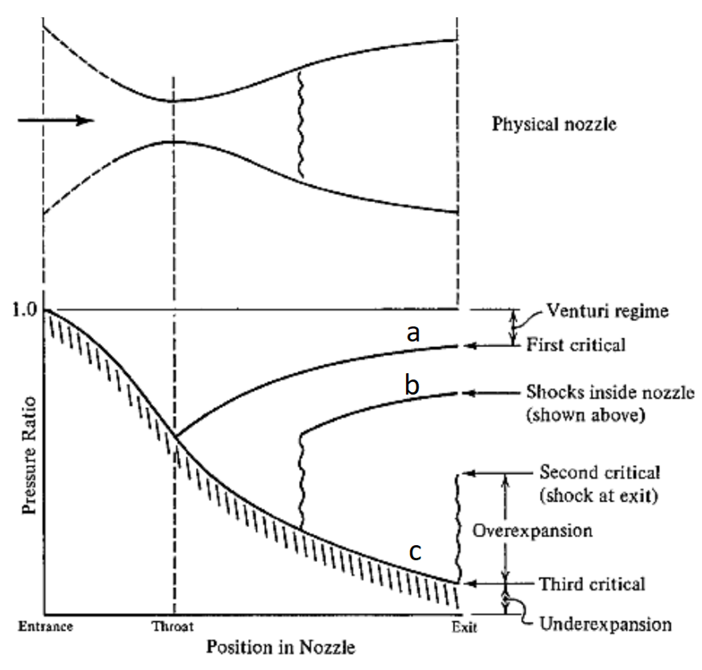
Figure 3.
Flow phenomena outside an a) underexpanded and b)overexpanded nozzle [5]
Figure 3.
Flow phenomena outside an a) underexpanded and b)overexpanded nozzle [5]
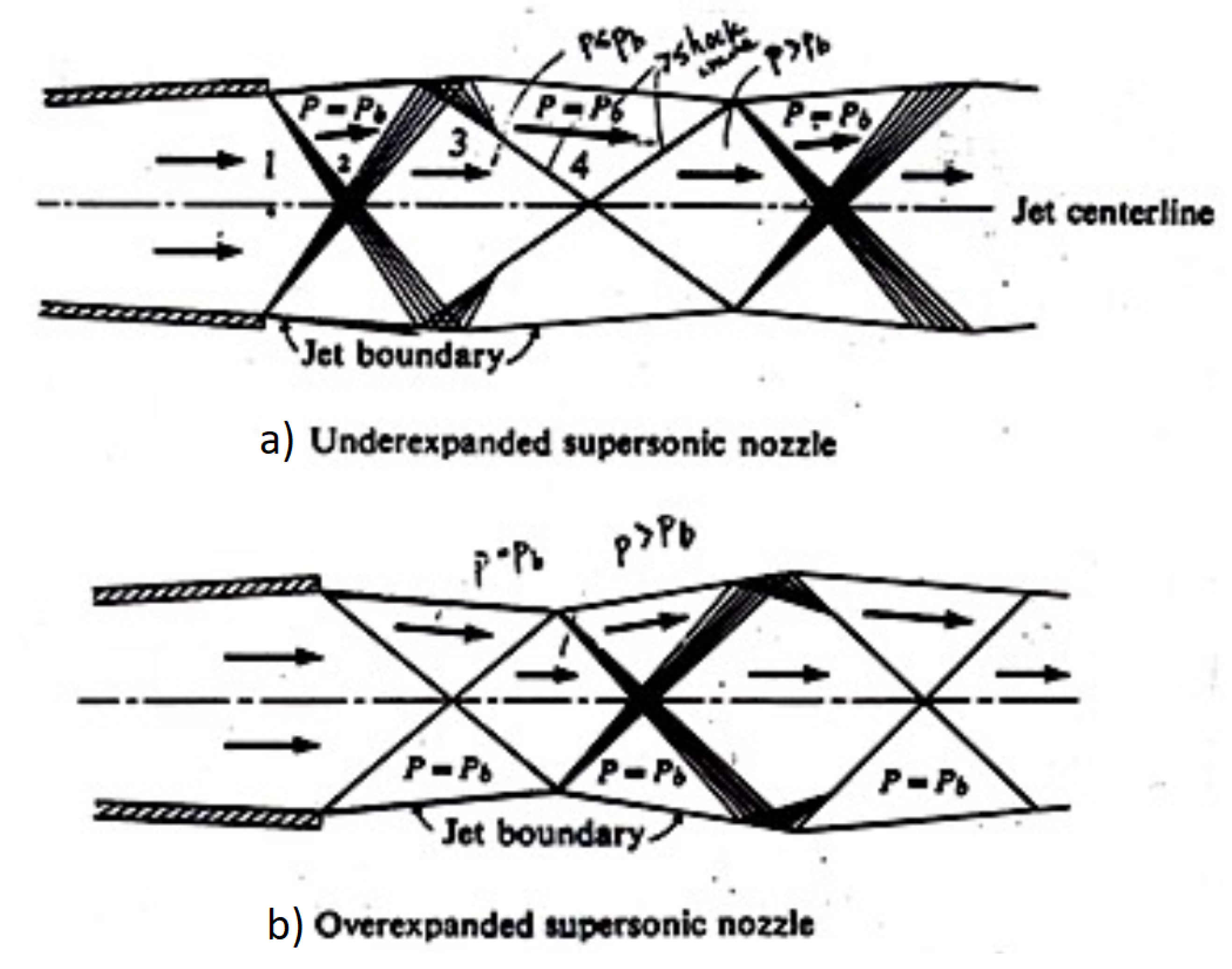
Figure 4.
Schematics of an oblique shock and properties variations
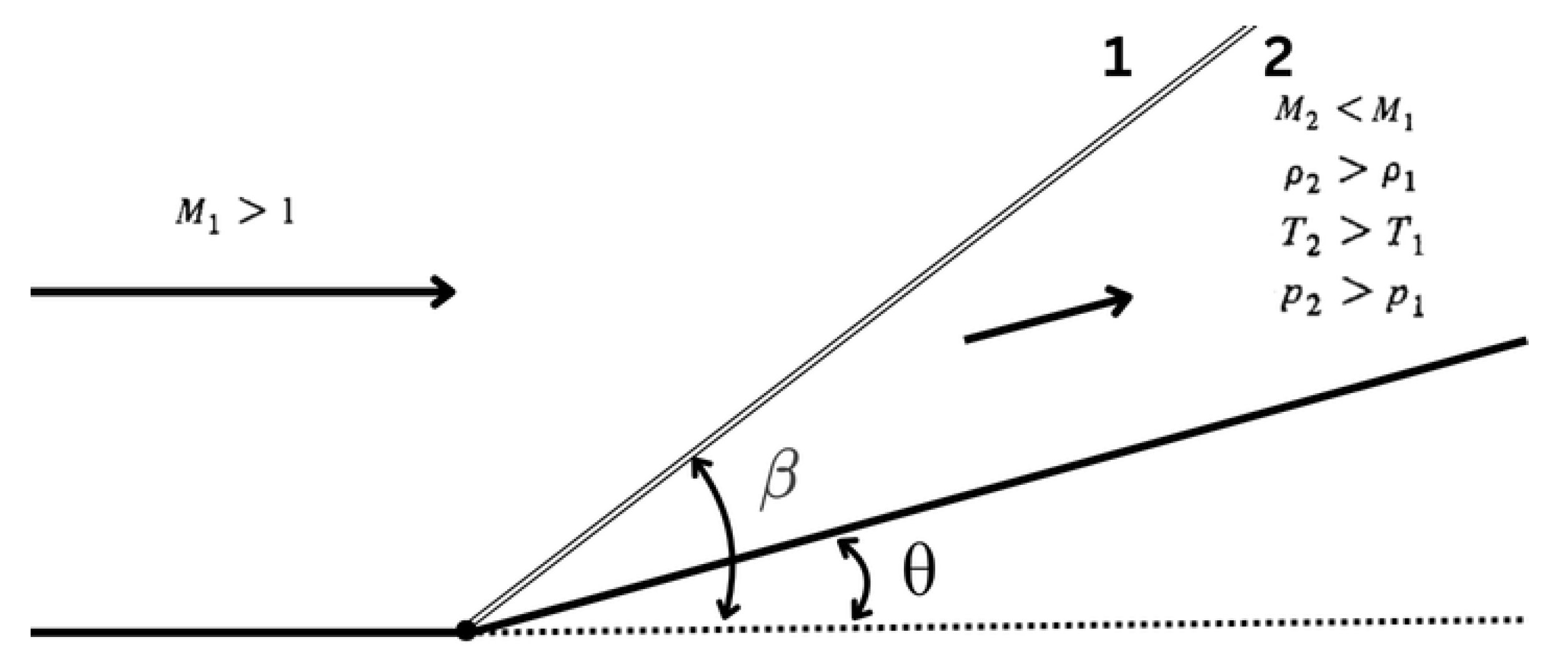
Figure 5.
Oblique shock - Relation between , and Mach number [6]
Figure 5.
Oblique shock - Relation between , and Mach number [6]
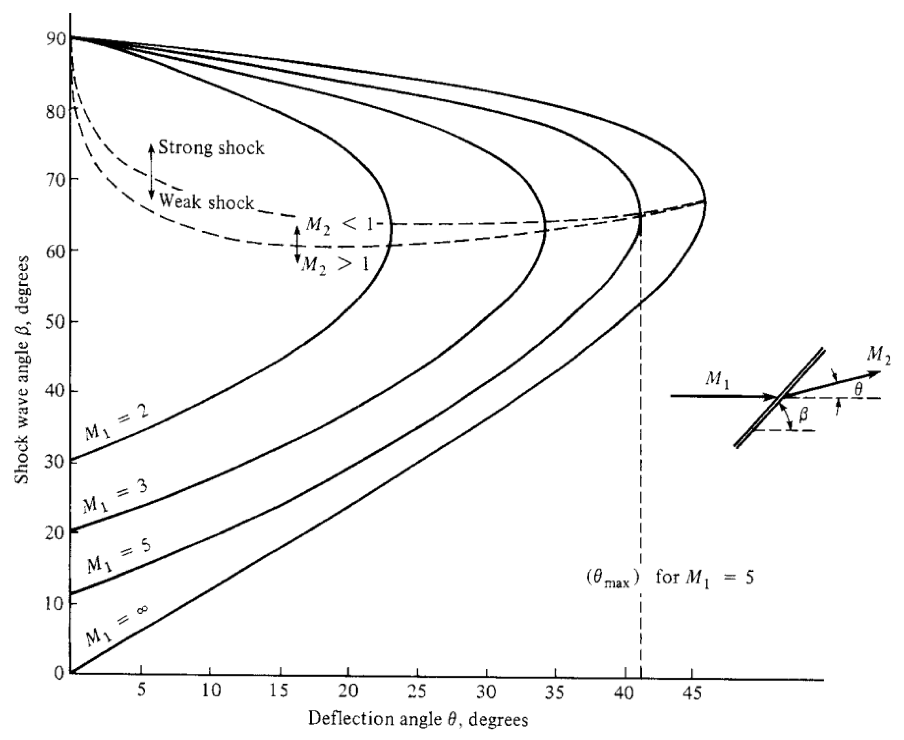
Figure 6.
Schematics of a Prandtl-Meyer expansion centered fan and properties variations through it
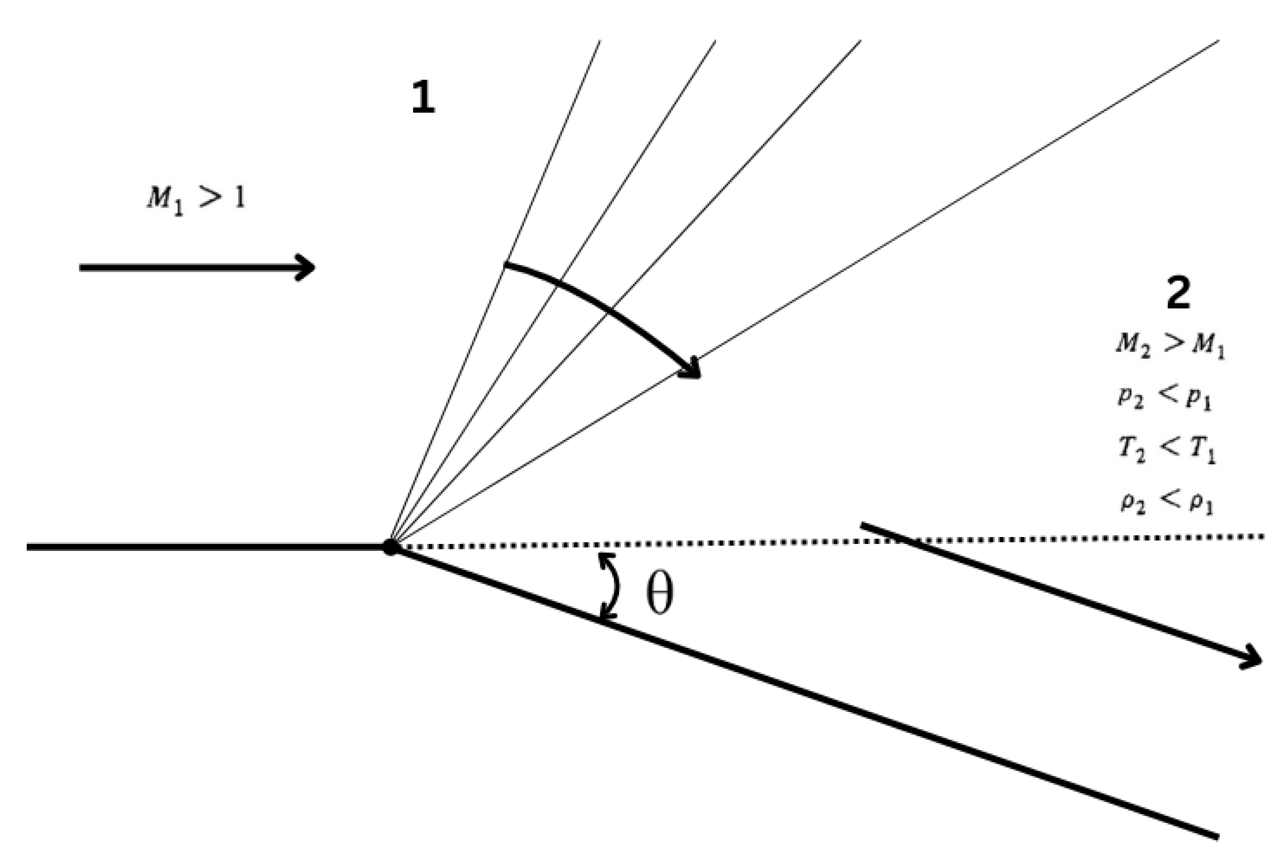
Figure 7.
Thin Shock Layer of Hypersonic Flow
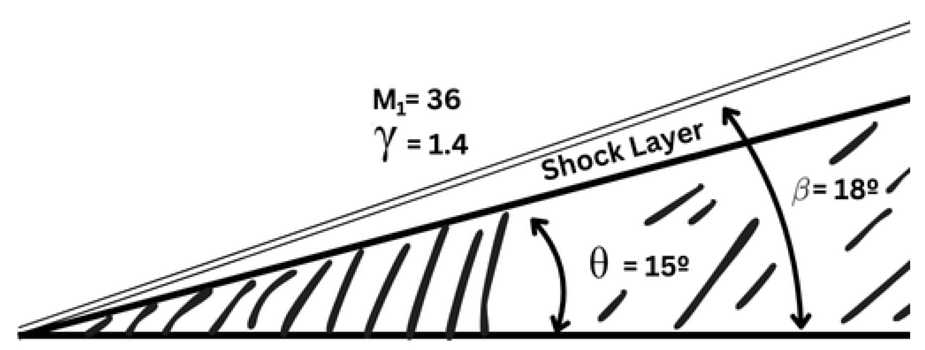
Figure 8.
Temperature Profile Within Hypersonic Boundary-Layer [6]
Figure 8.
Temperature Profile Within Hypersonic Boundary-Layer [6]
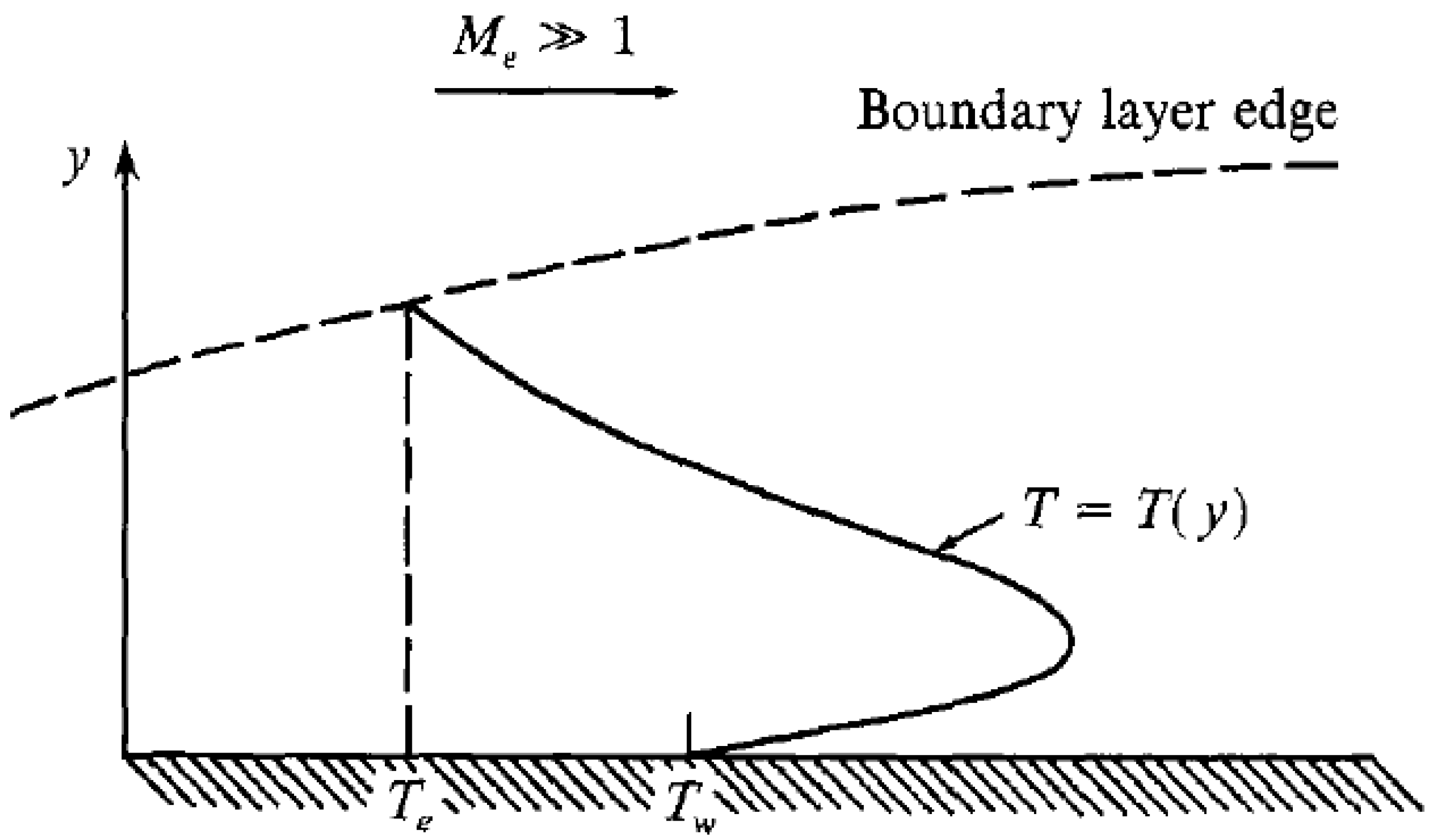
Figure 9.
Comparison of Newtonian Theory Pressure Coefficient v.s. Freestream Mach Number [6]
Figure 9.
Comparison of Newtonian Theory Pressure Coefficient v.s. Freestream Mach Number [6]
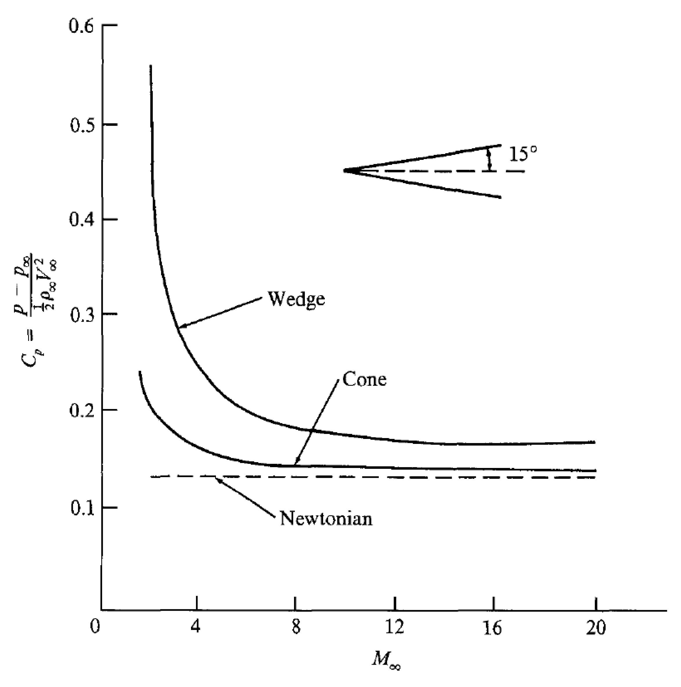
Figure 10.
Modes of Molecular Energies (’) for Diatomic Molecules
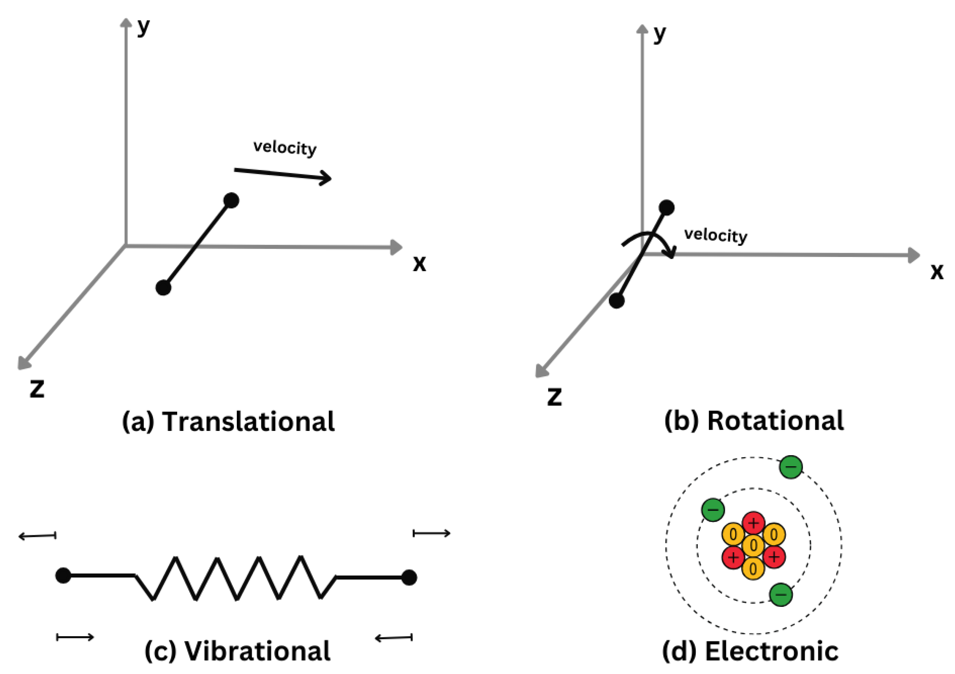
Figure 11.
Visual Example of Degenerated States within a Energy Level
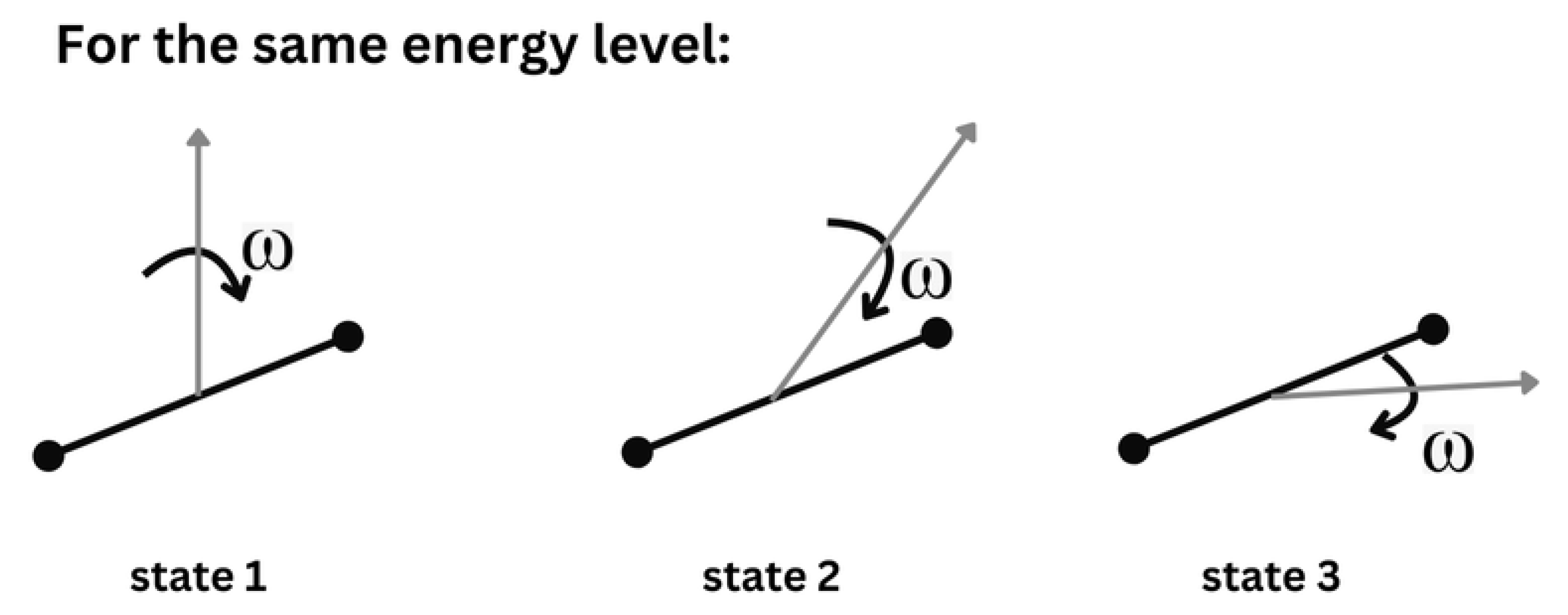
Figure 12.
Specific Heat at Constant Volume v.s. Temperature (K) [6]
Figure 12.
Specific Heat at Constant Volume v.s. Temperature (K) [6]
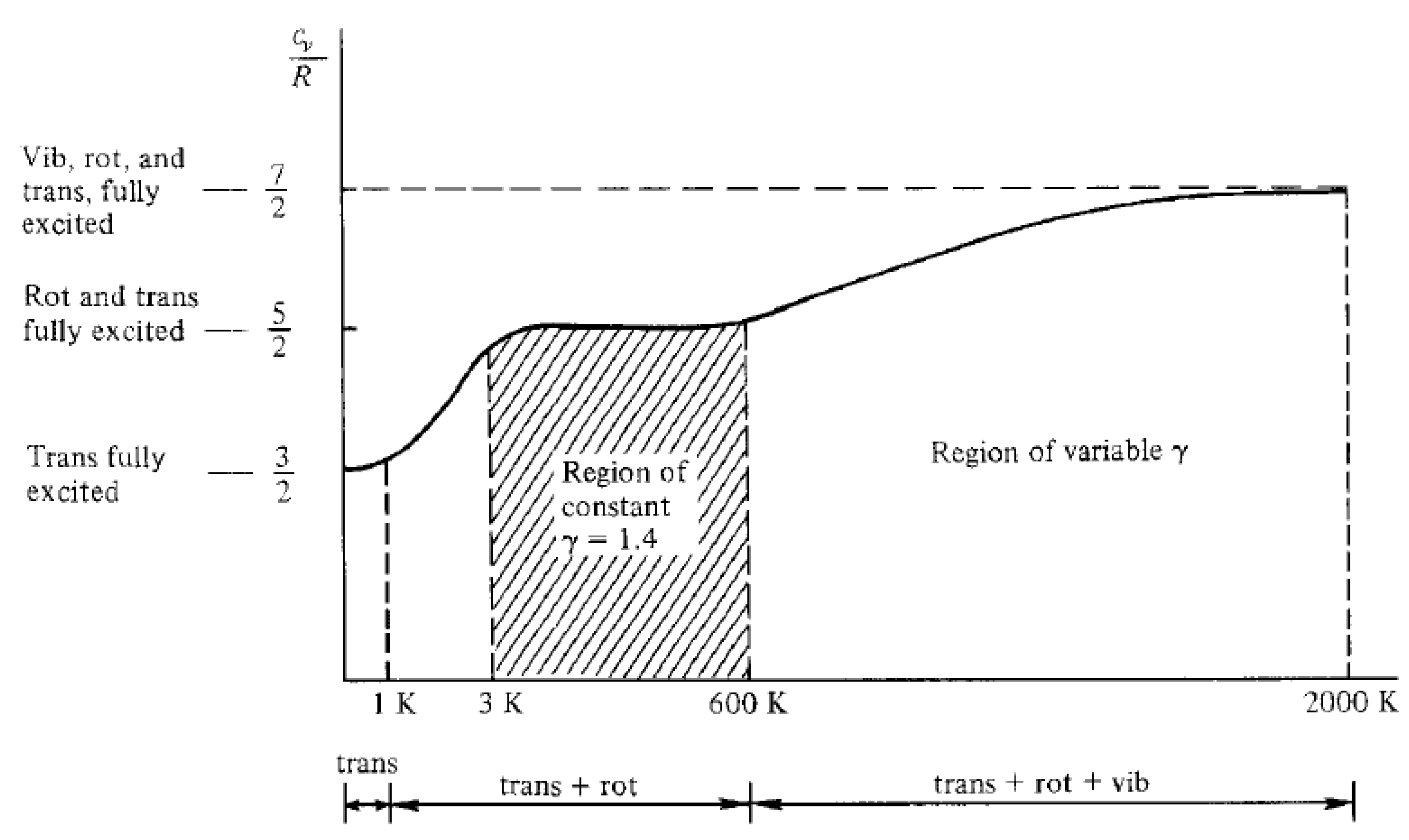
Figure 13.
Difference between Sensible Enthalpy and Zero-point Energy [6]
Figure 13.
Difference between Sensible Enthalpy and Zero-point Energy [6]
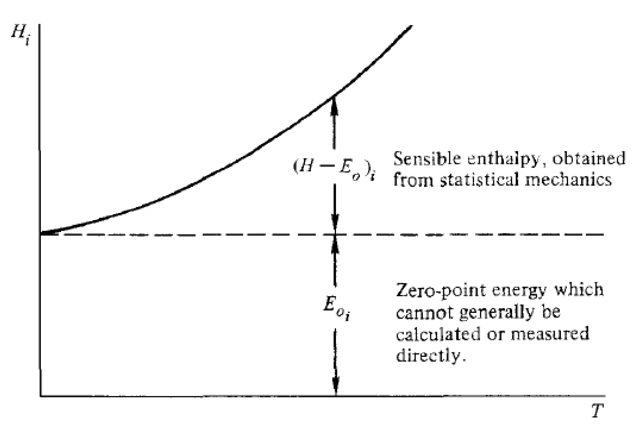
Figure 14.
Chemical Composition of the Gas Through a de Laval Nozzle [6]
Figure 14.
Chemical Composition of the Gas Through a de Laval Nozzle [6]
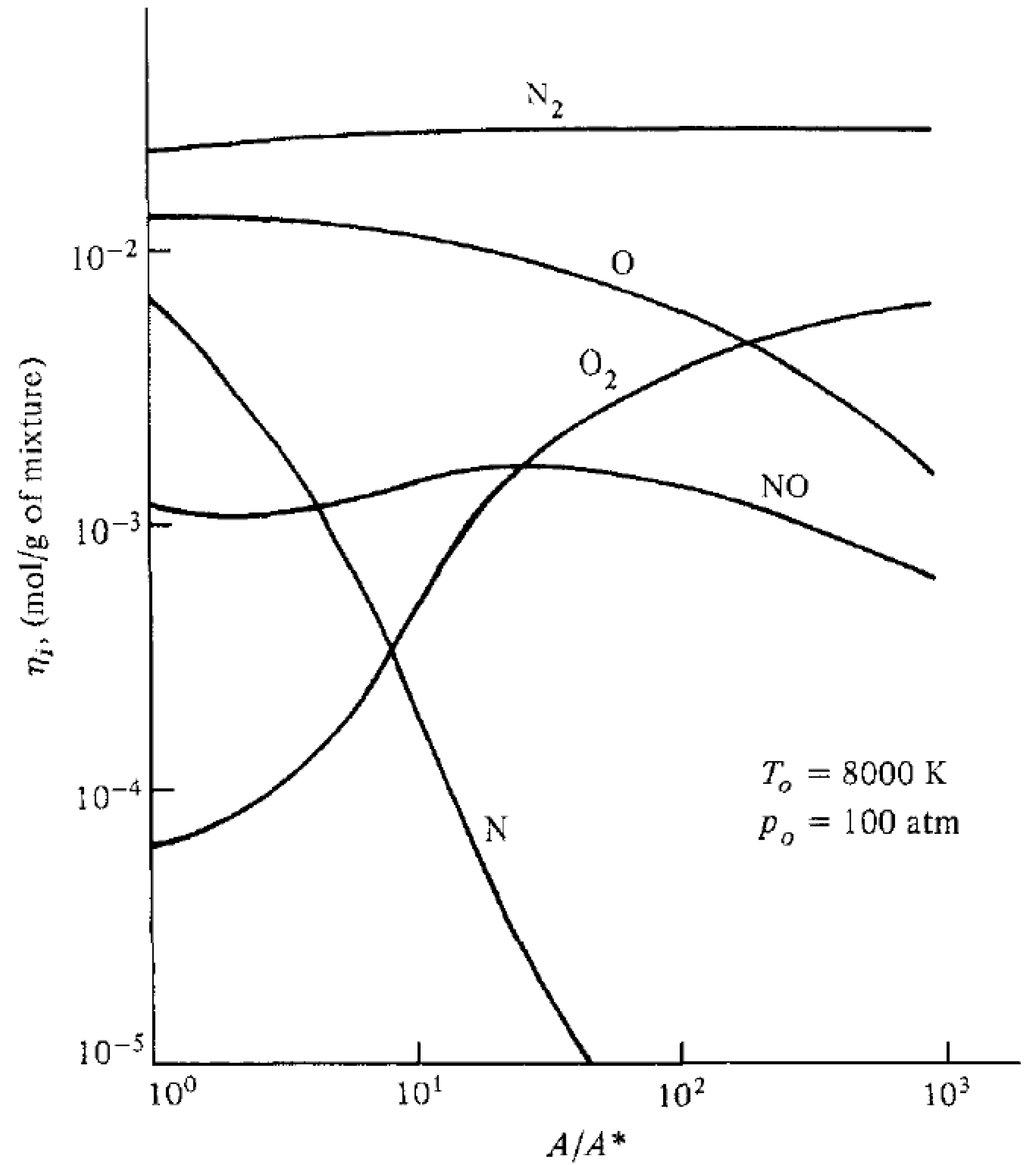
Figure 15.
Transonic Line with (a) several methods [10] and (b) In-House algorithm with Dutton’s method
Figure 15.
Transonic Line with (a) several methods [10] and (b) In-House algorithm with Dutton’s method
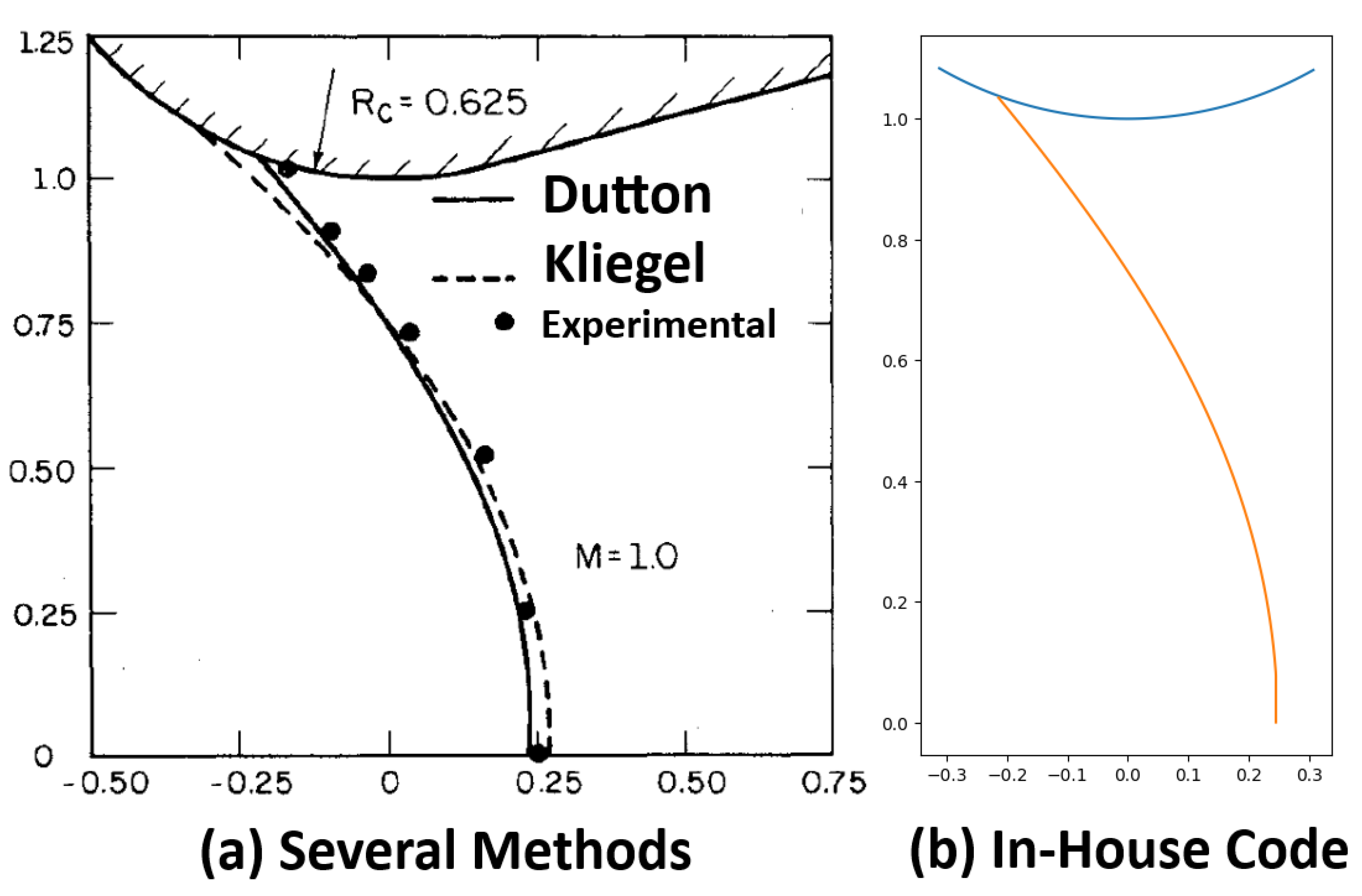
Figure 16.
Characteristic lines passing a given point of a supersonic flow
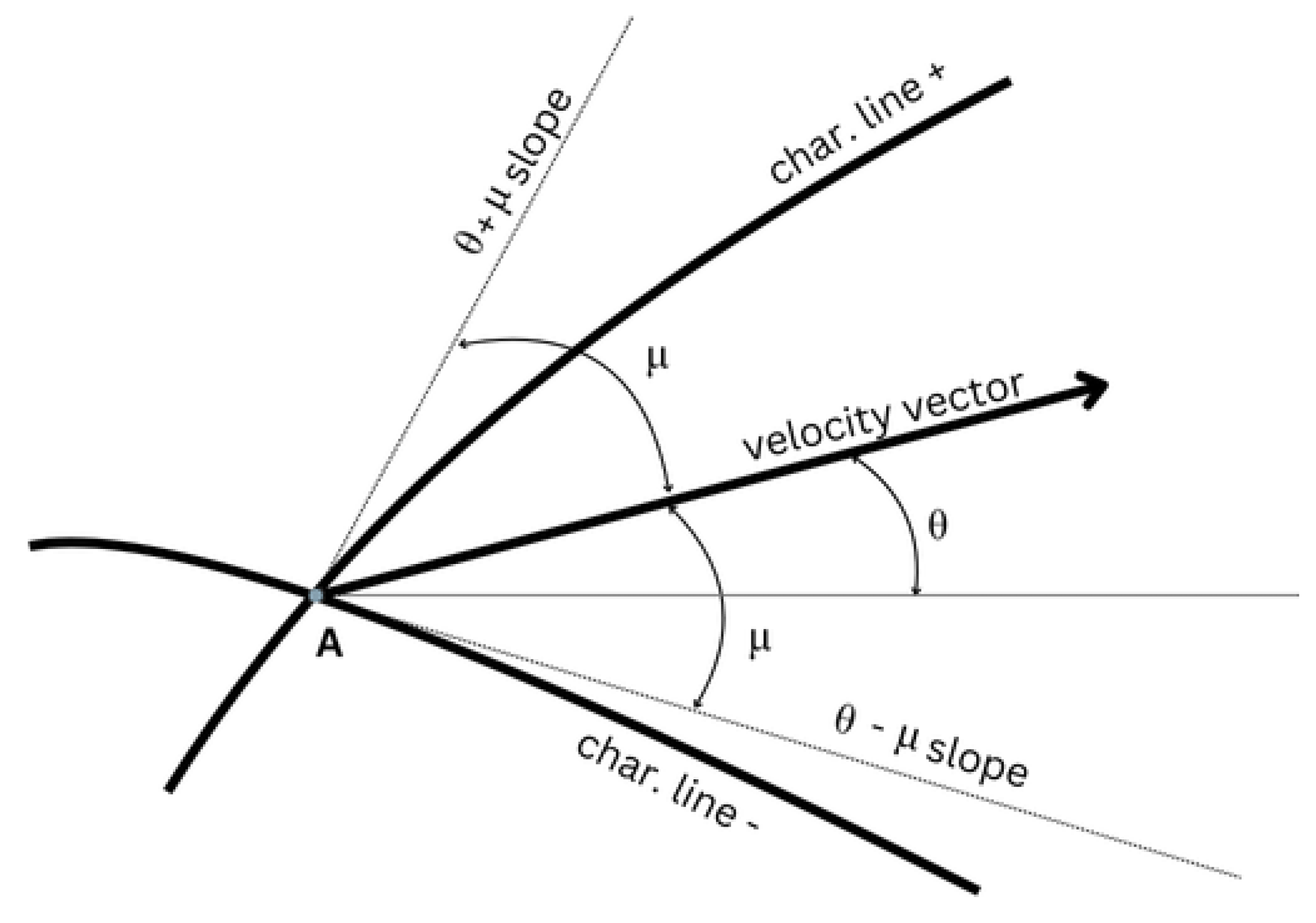
Figure 17.
Rectangular finite-difference grid
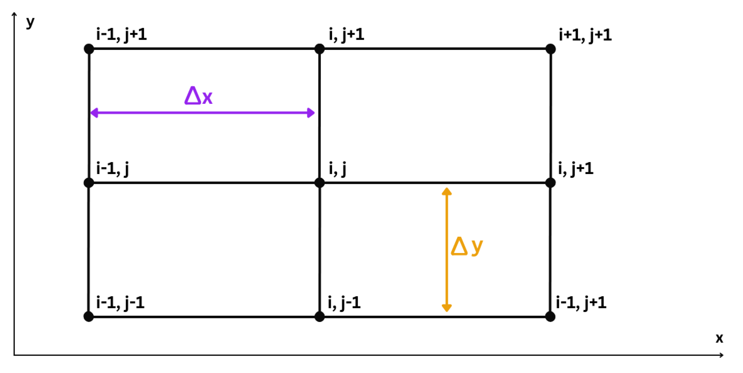
Figure 18.
Shock and wall boundary conditions for supersonic steady-flow finite-difference solutions [6]
Figure 18.
Shock and wall boundary conditions for supersonic steady-flow finite-difference solutions [6]
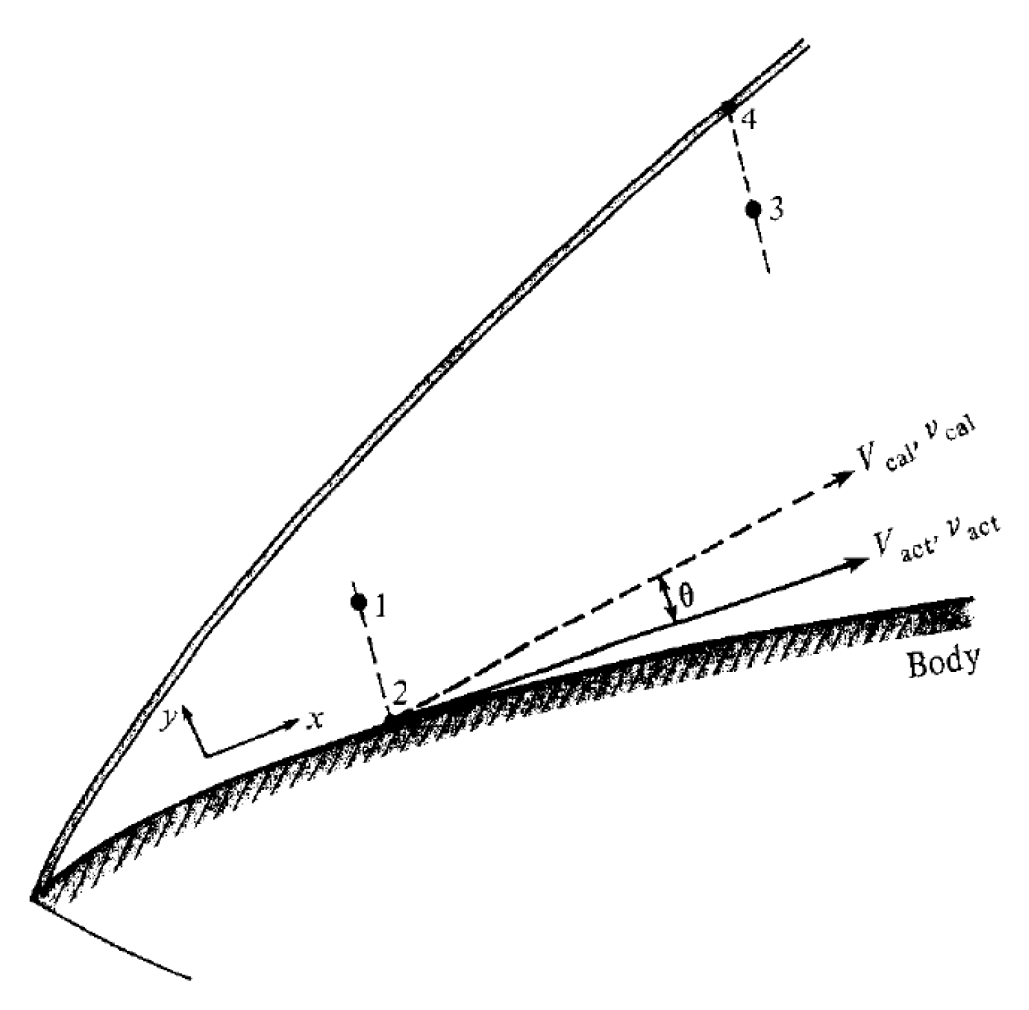
Figure 19.
Meshes for the a) shock-fitting and b) shock-capturing finite-difference [6]
Figure 19.
Meshes for the a) shock-fitting and b) shock-capturing finite-difference [6]
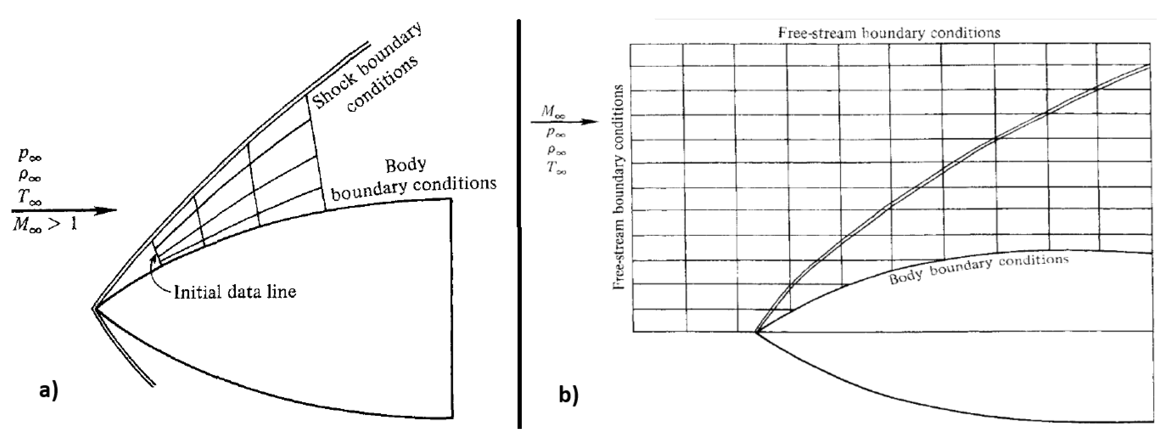
Figure 20.
Velocity fluctuations in a fixed point of a turbulent flow [16]
Figure 20.
Velocity fluctuations in a fixed point of a turbulent flow [16]
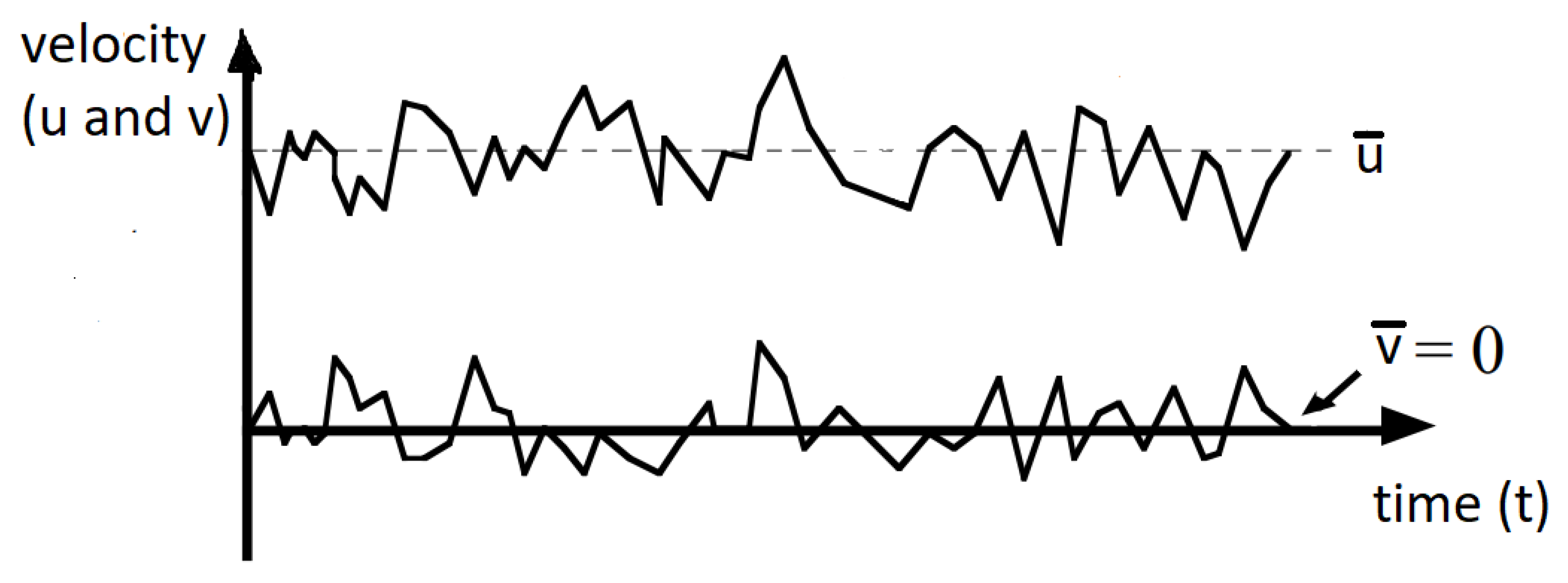
Figure 21.
Conical nozzle’s configuration [2]
Figure 21.
Conical nozzle’s configuration [2]
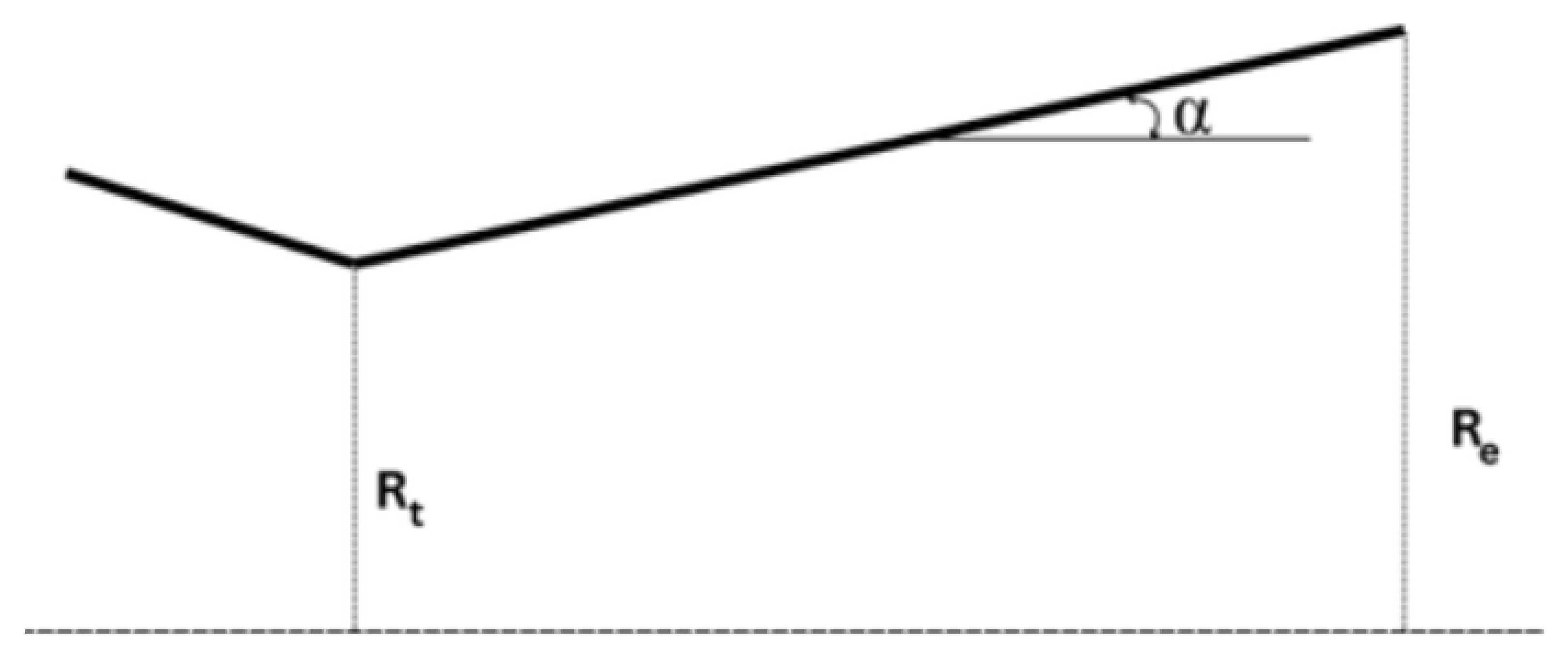
Figure 22.
Assumption of the Flow Inside a Conical Nozzle
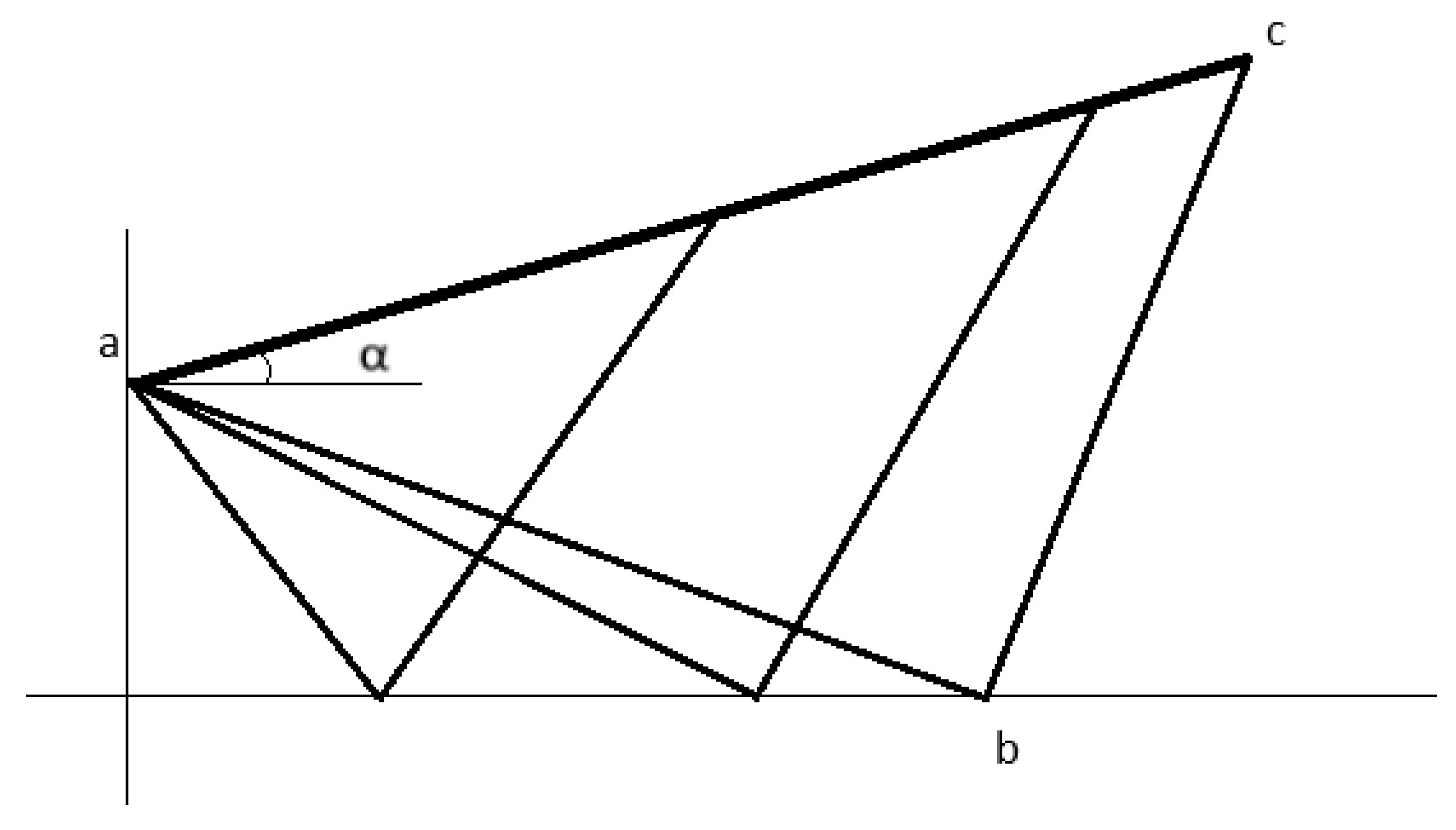
Figure 23.
Characteristic Lines Inside a 2D Ramp Designed for and
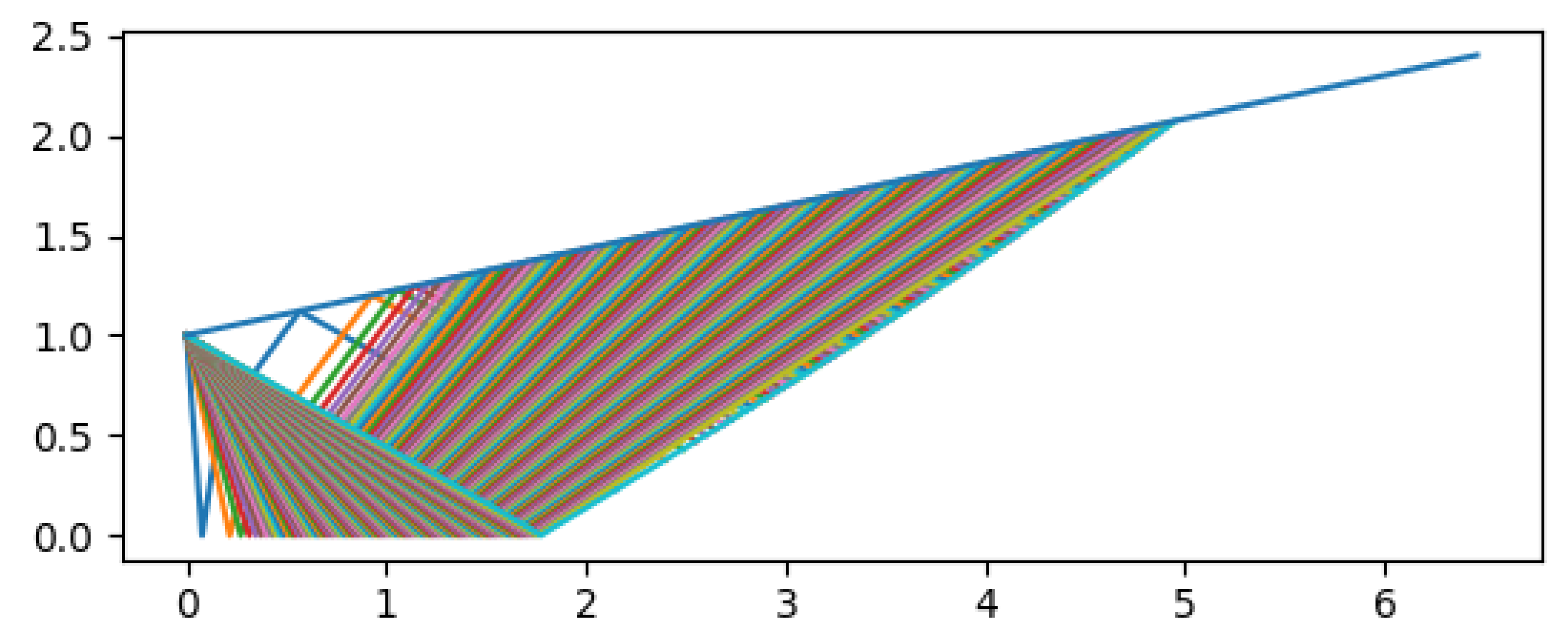
Figure 24.
CFD Depiction of the Flow Inside Conical Nozzle Operating at Design Conditions [29]
Figure 24.
CFD Depiction of the Flow Inside Conical Nozzle Operating at Design Conditions [29]
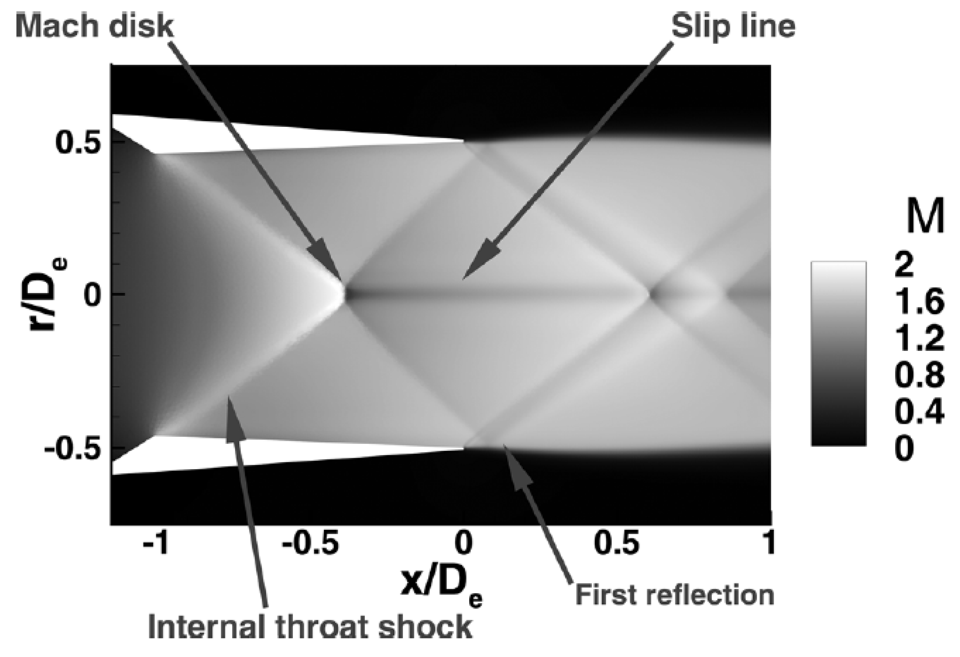
Figure 25.
Bell nozzle’s configuration and comparison with conical nozzle [2]
Figure 25.
Bell nozzle’s configuration and comparison with conical nozzle [2]
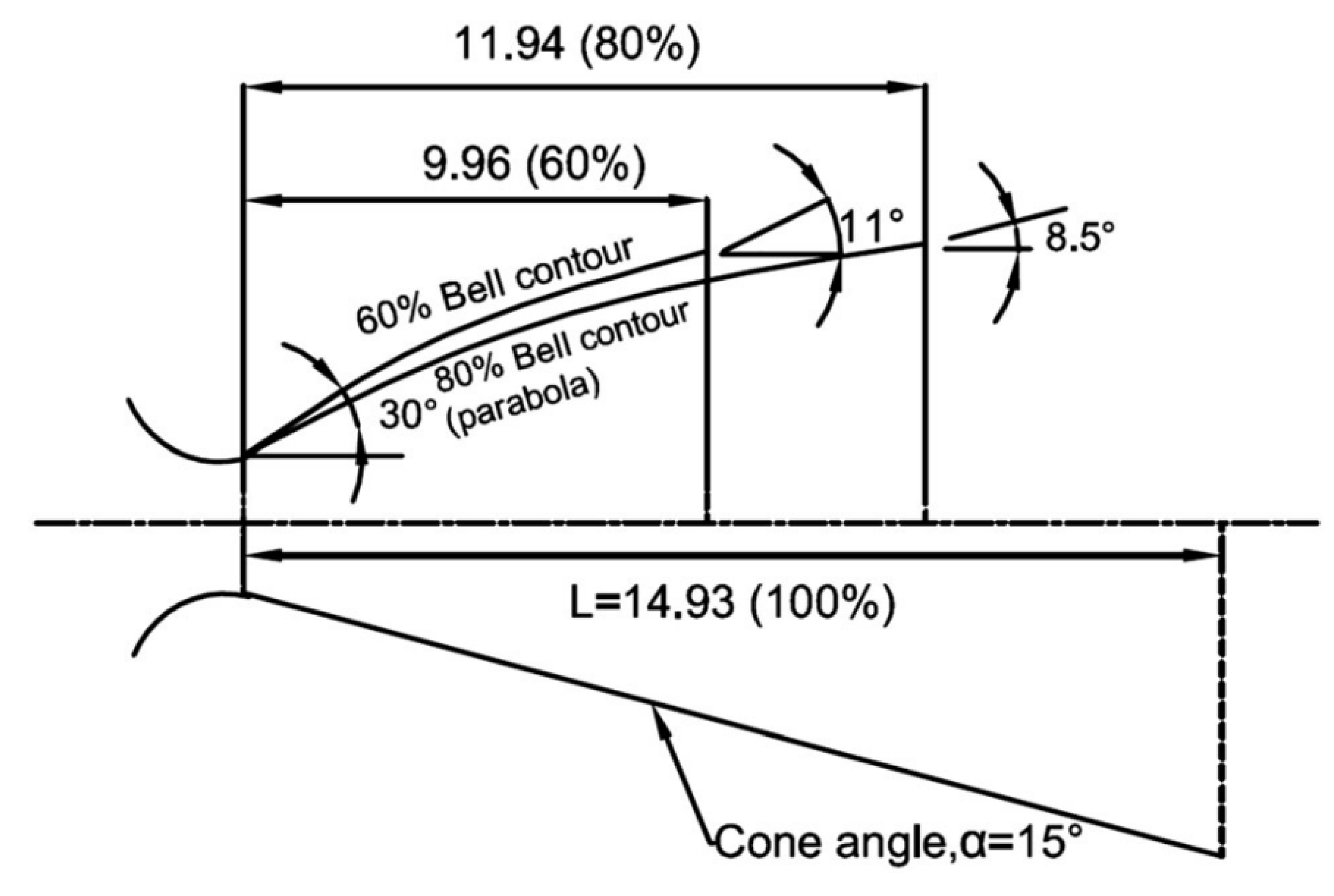
Figure 26.
Minimum Length Bell Nozzle Design [6]
Figure 26.
Minimum Length Bell Nozzle Design [6]
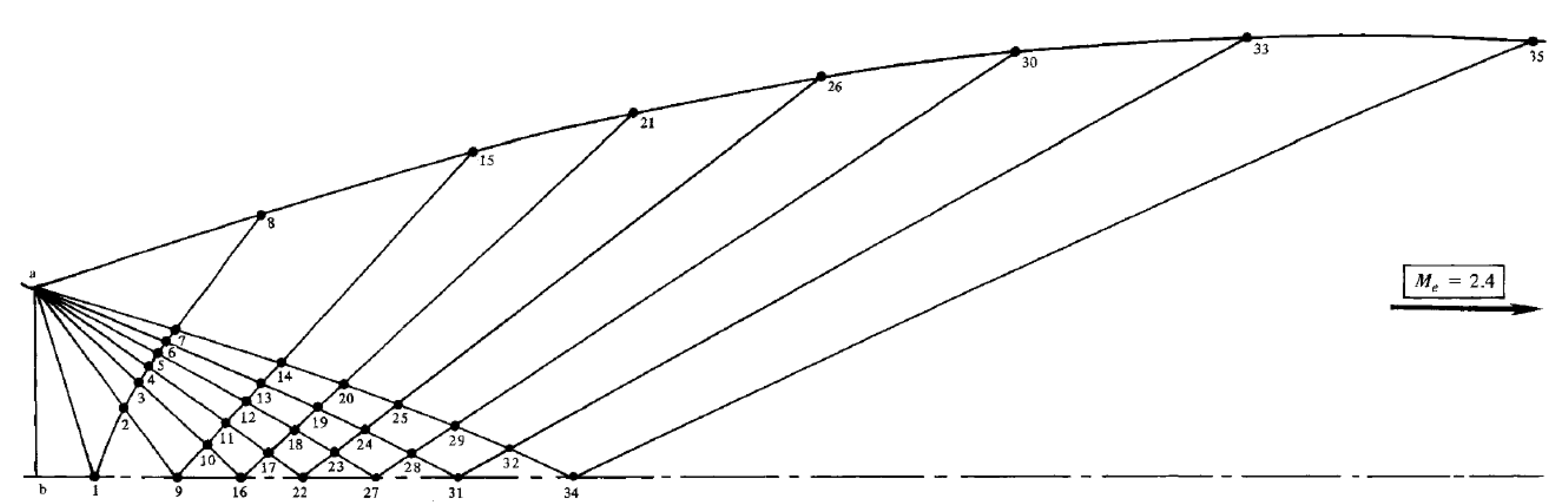
Figure 27.
Minimum Length 2D Bell Nozzle from In-House Code
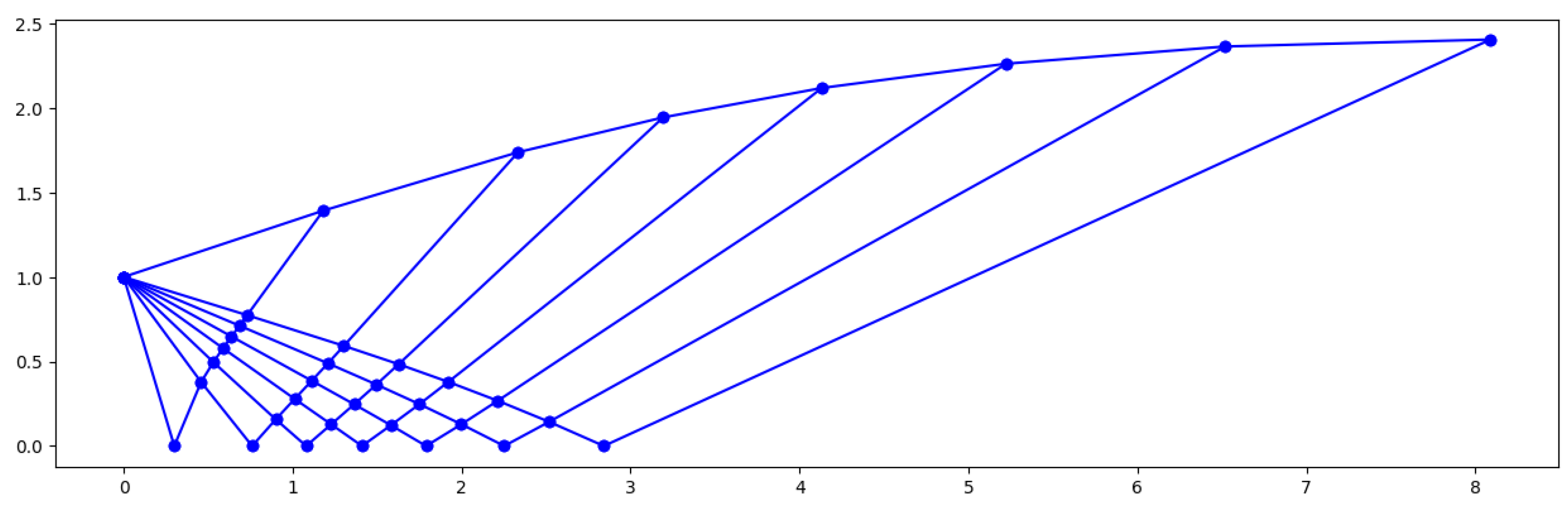
Figure 28.
Minimum Length Bell Nozzle with Boundary-Layer Correction for Thermically Perfect Gas
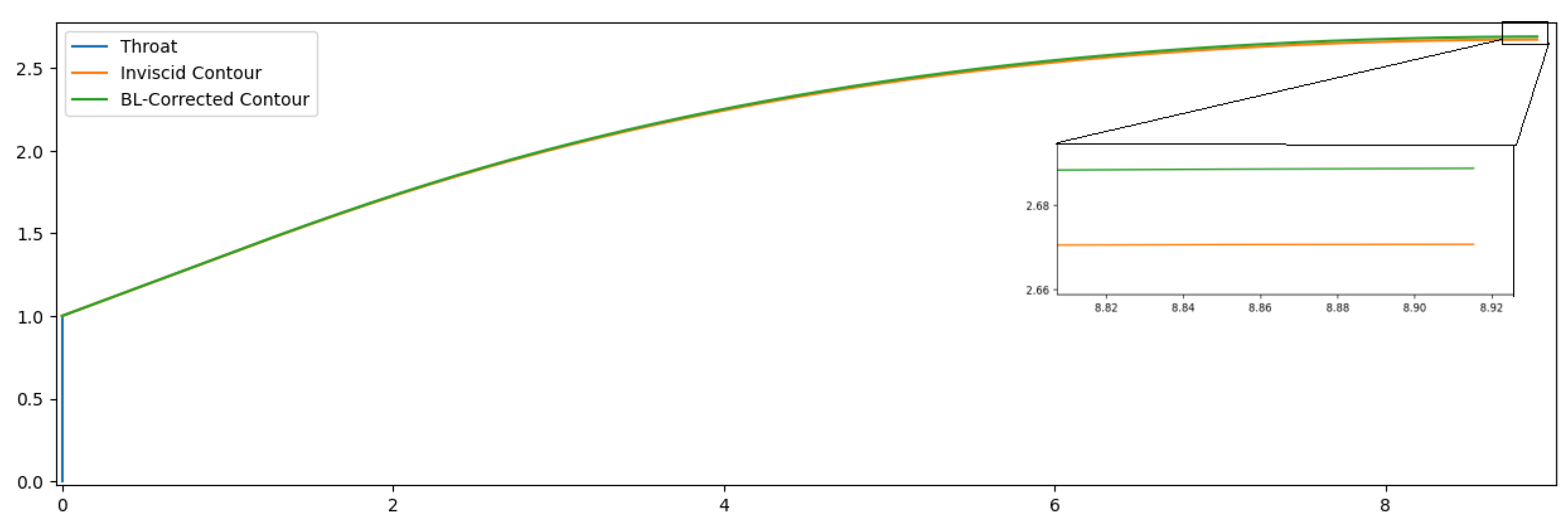
Figure 29.
Minimum Length Axisymetric Bell Nozzle Design [12]
Figure 29.
Minimum Length Axisymetric Bell Nozzle Design [12]
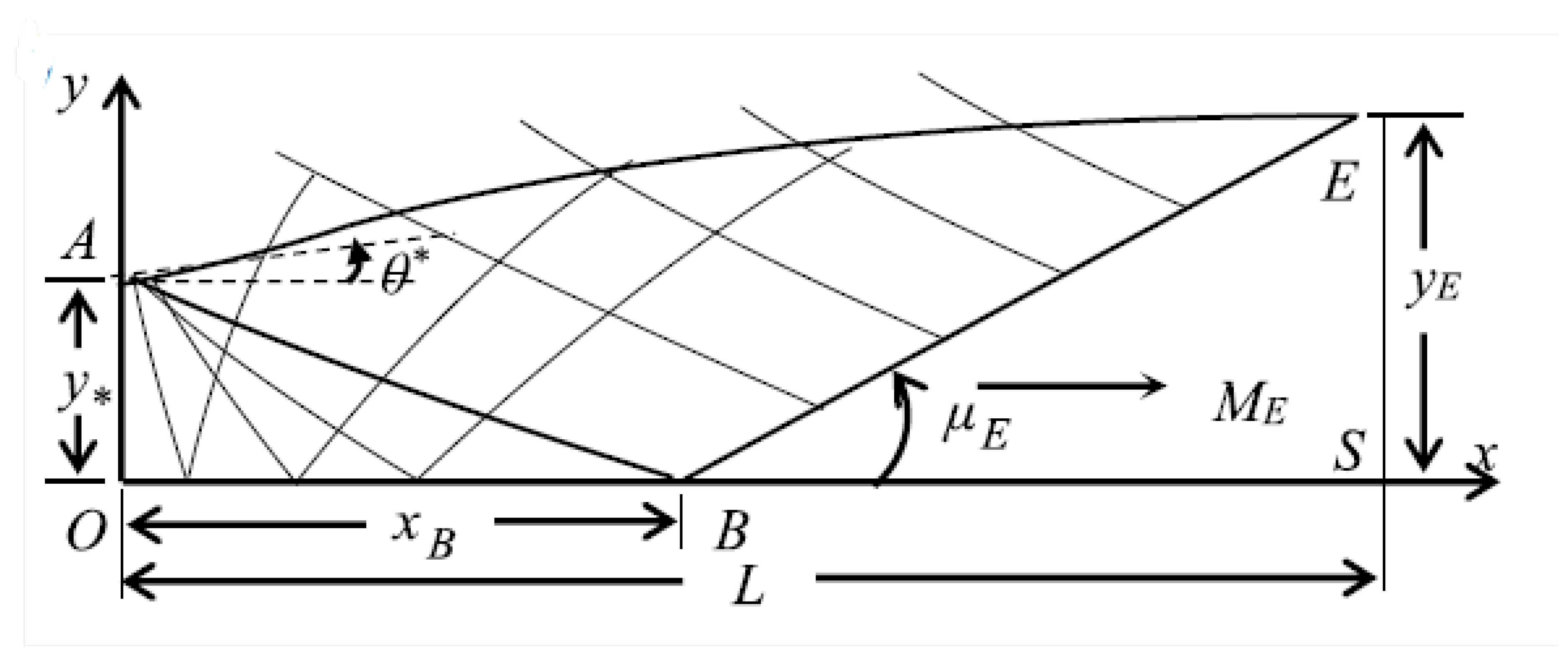
Figure 30.
Characteristics grids for , and 7 lines
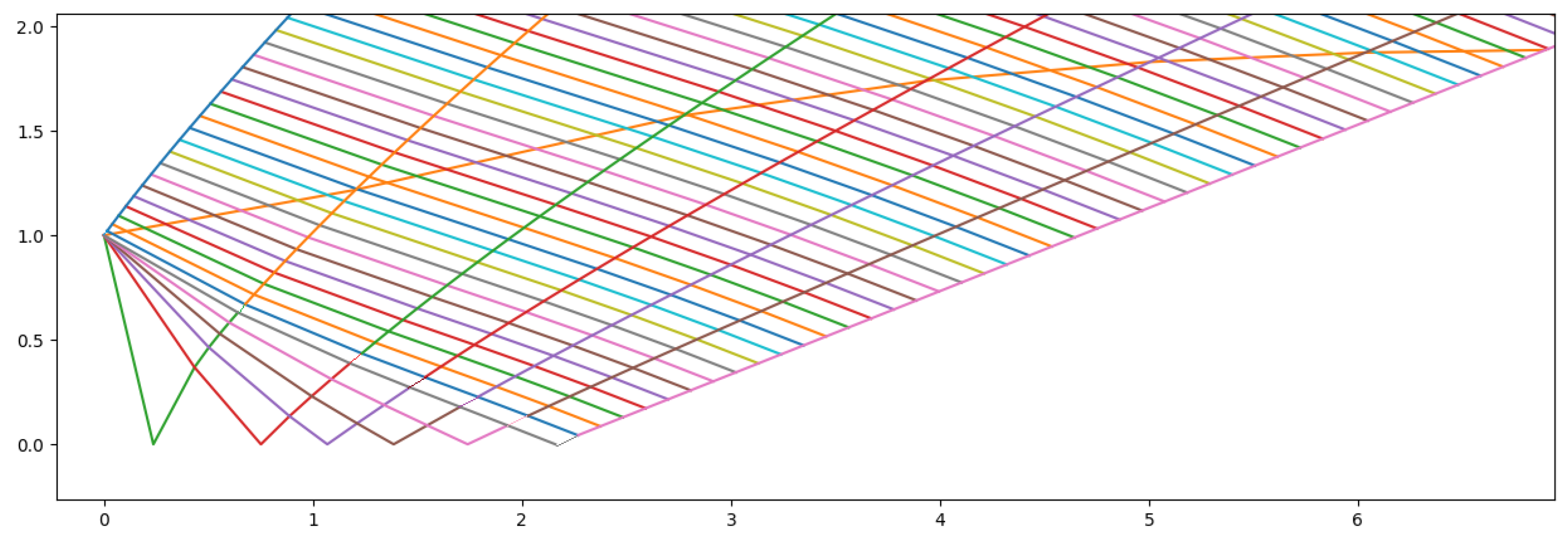
Figure 31.
Contour for , and 100 lines from (a) Reference [13] and (b) in-house code
Figure 31.
Contour for , and 100 lines from (a) Reference [13] and (b) in-house code
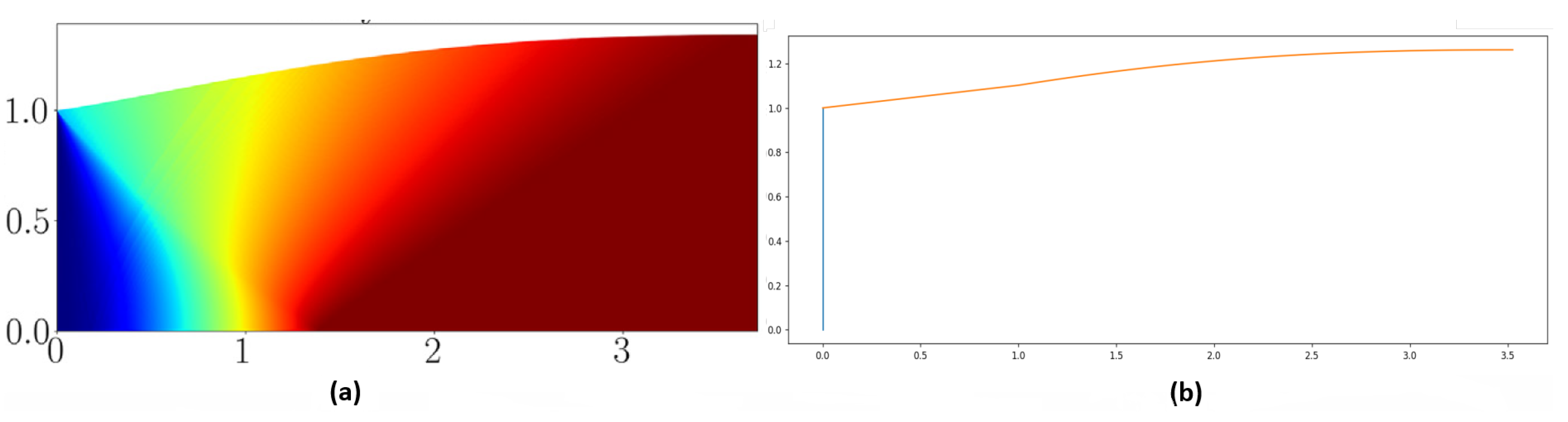
Figure 32.
Sketch of a Parabolic Bell Nozzle
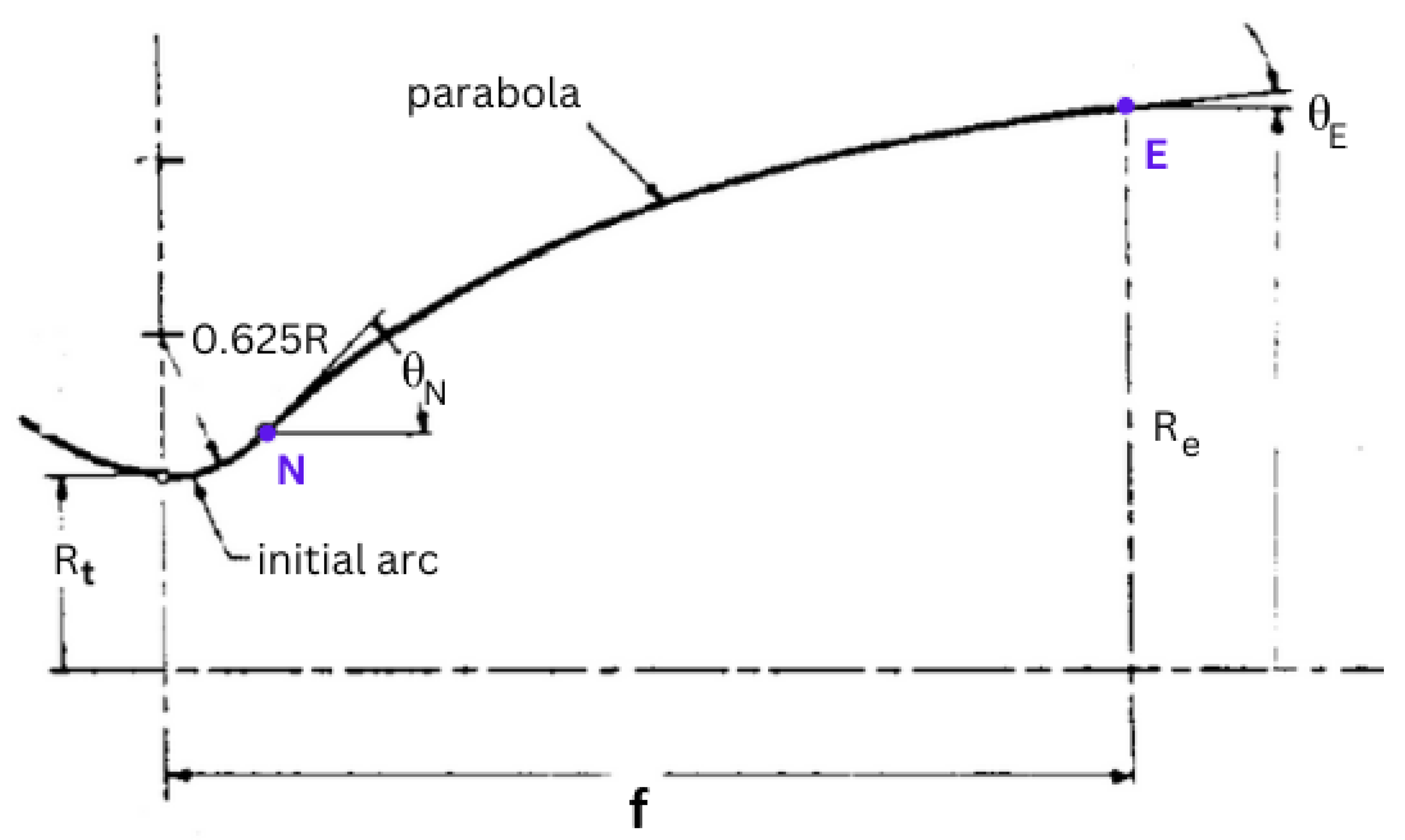
Figure 33.
Points necessary to draw a parabola [35]
Figure 33.
Points necessary to draw a parabola [35]
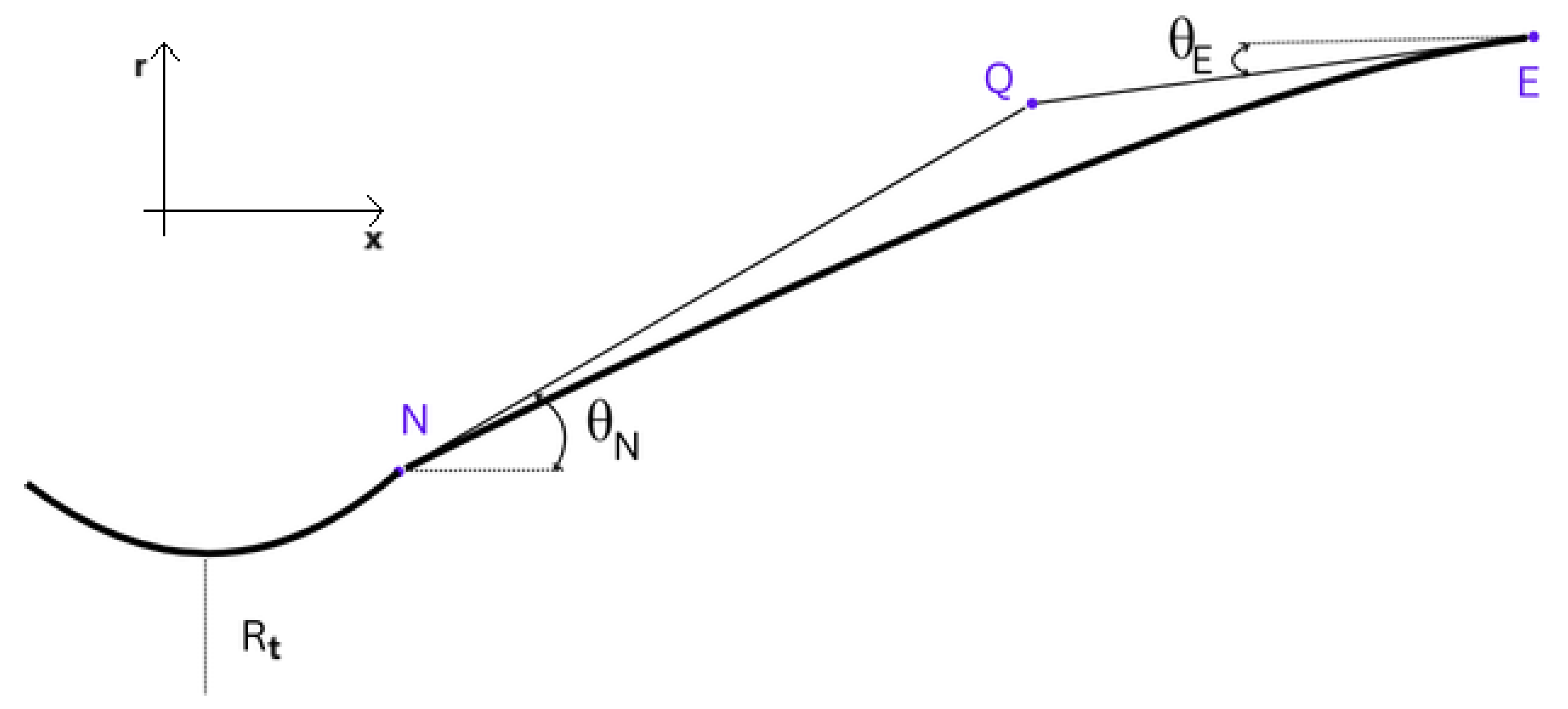
Figure 34.
Parabolic Bell Nozzle for , , , and of a 15º conical nozzle
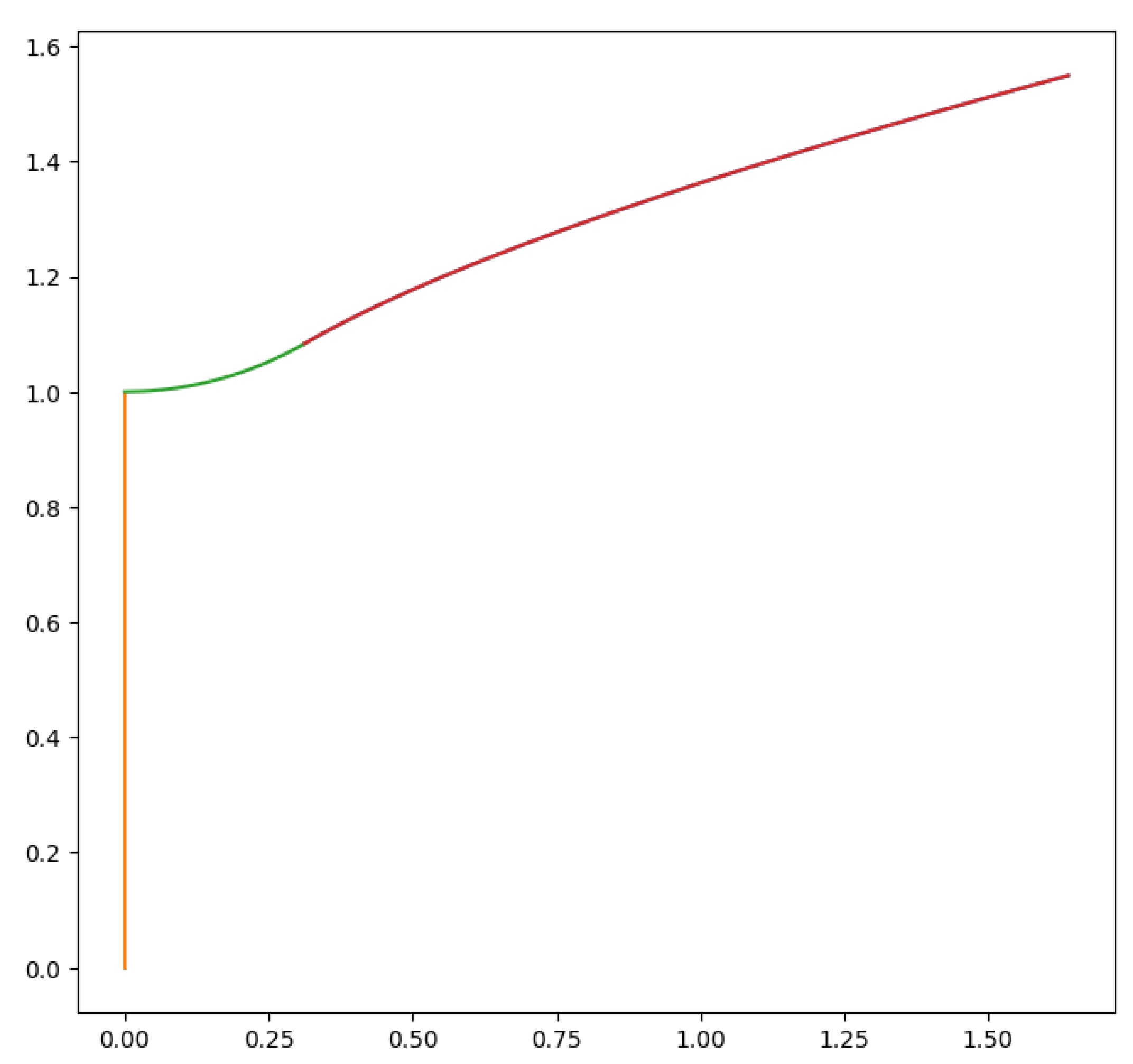
Figure 35.
In-house MOC code prediction of weak shock inside TOP nozzle
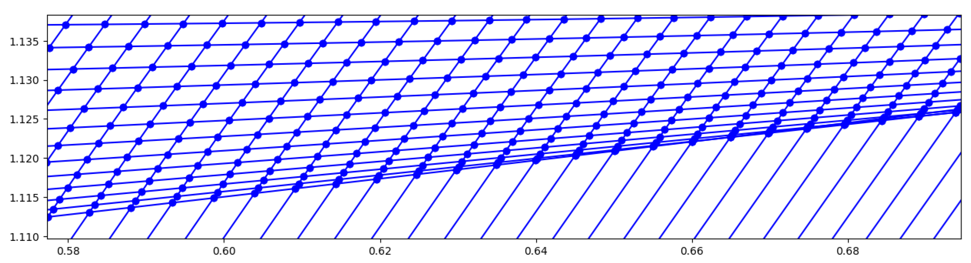
Figure 36.
Schematic of a) FSS and b) RSS condition inside a TOP nozzle [37]
Figure 36.
Schematic of a) FSS and b) RSS condition inside a TOP nozzle [37]
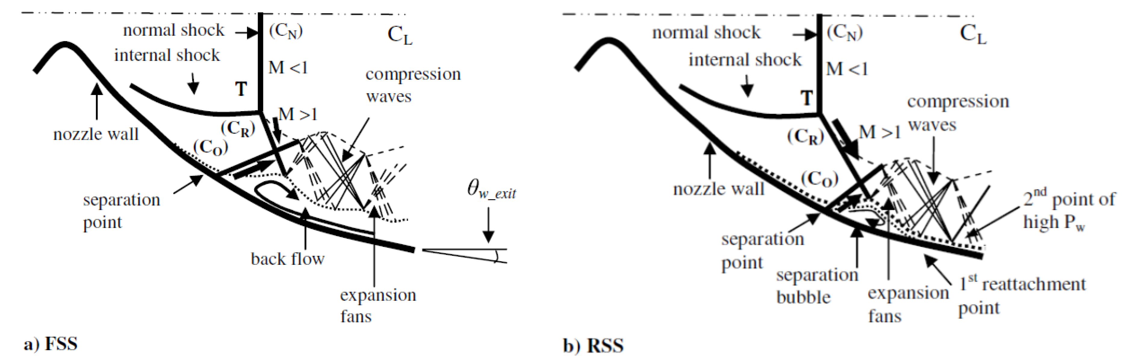
Figure 37.
TIC nozzle design steps [41]
Figure 37.
TIC nozzle design steps [41]
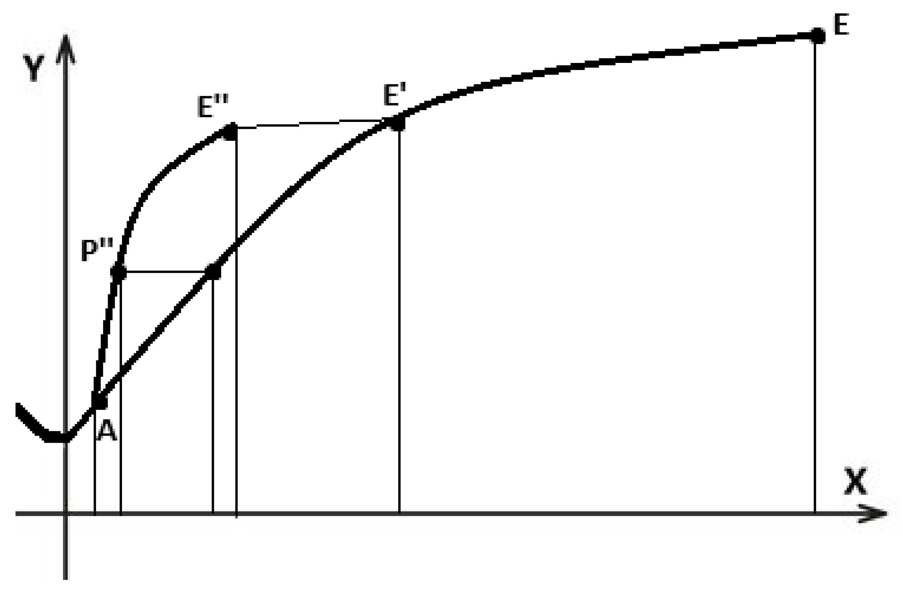
Figure 38.
TIC nozzle results for several design steps
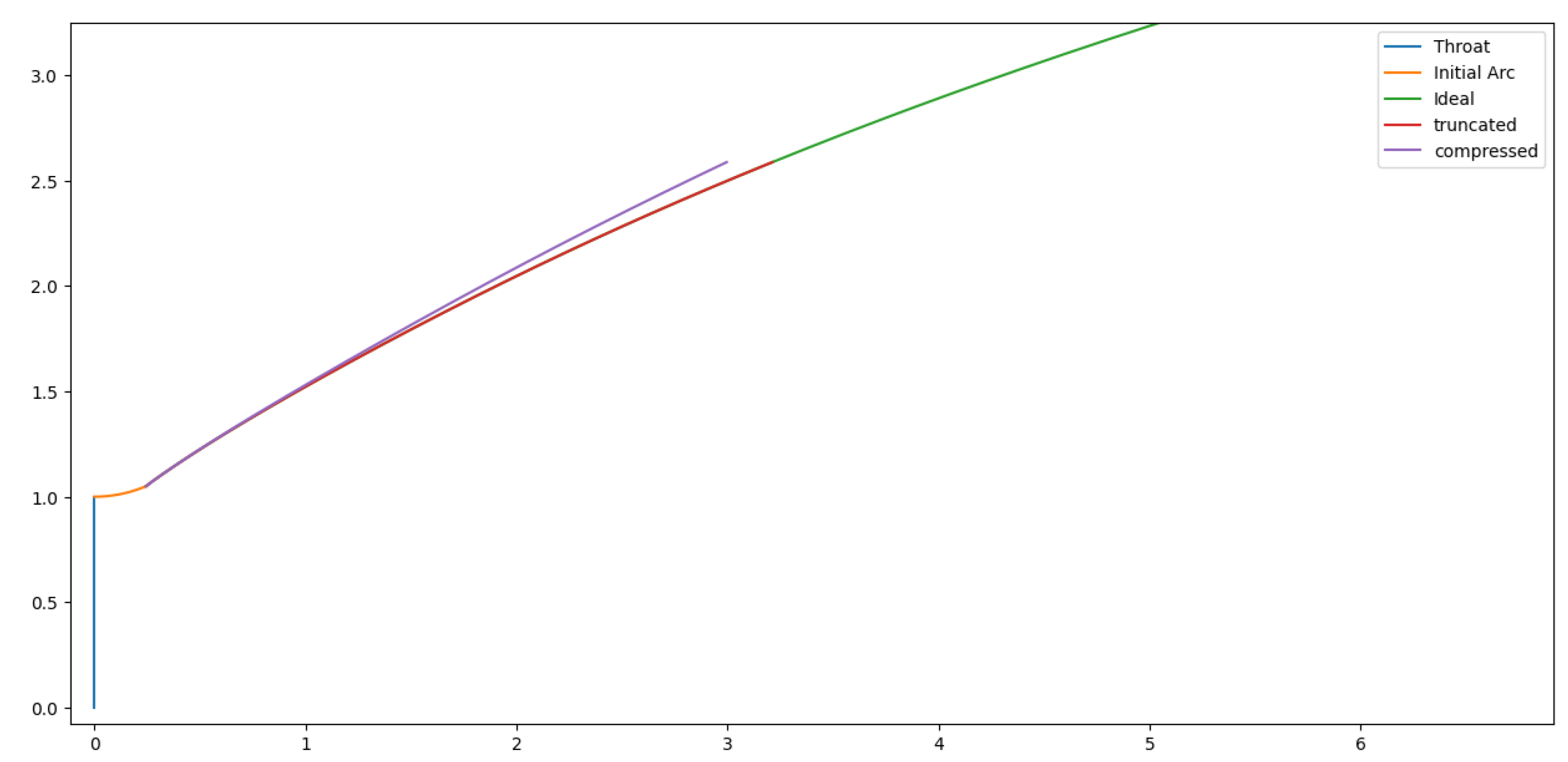
Figure 39.
TIC nozzle from in-house code
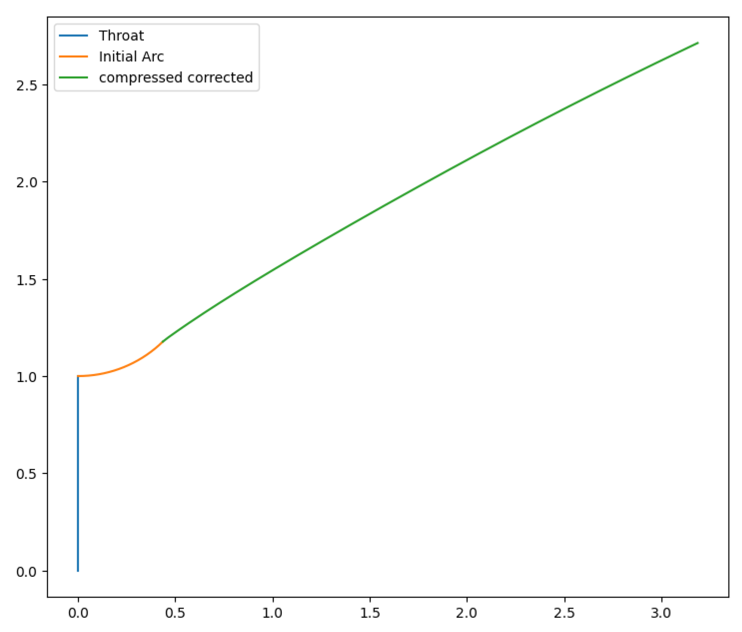
Figure 40.
In-house MOC code prediction of weak shock inside TIC nozzle
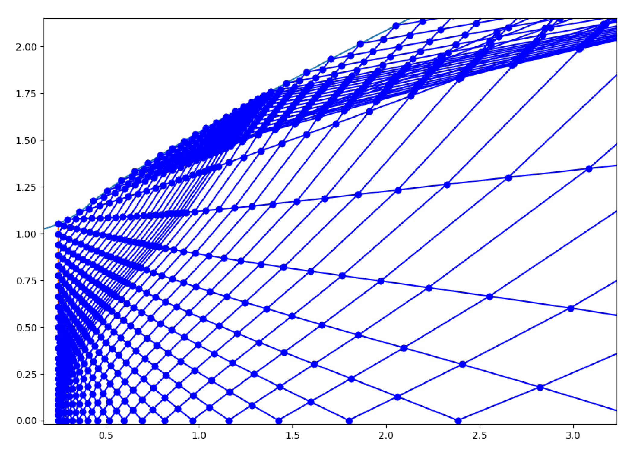
Figure 41.
Schematics of Supersonic Wind Tunnel
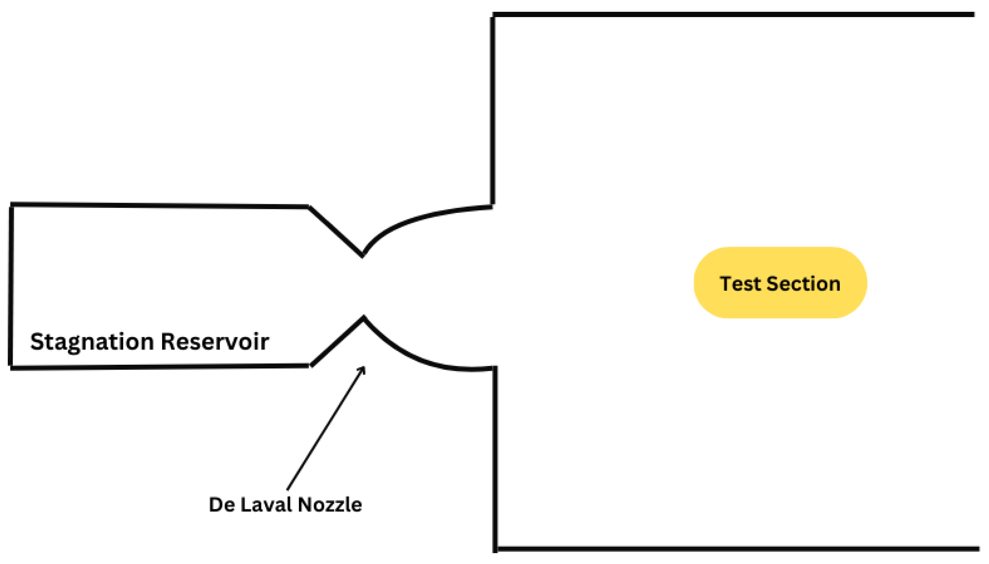
Figure 42.
Contour to convert radial flow into parallel flow [45]
Figure 42.
Contour to convert radial flow into parallel flow [45]
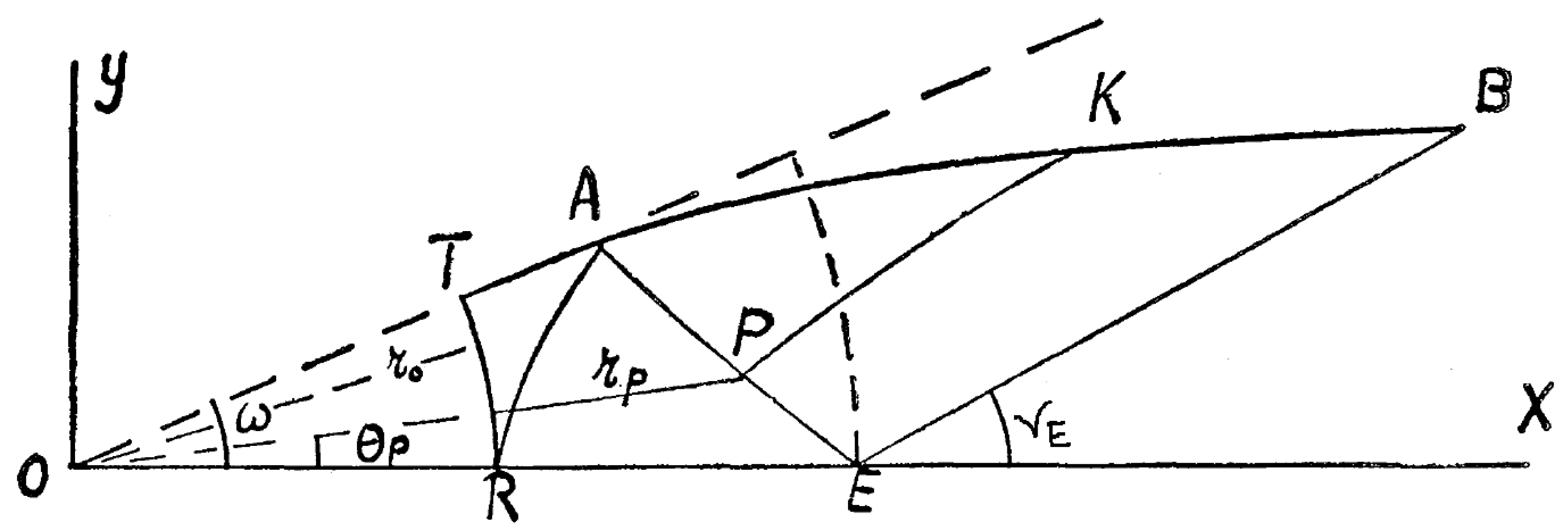
Figure 43.
Foelsch nozzle scheme [45]
Figure 43.
Foelsch nozzle scheme [45]
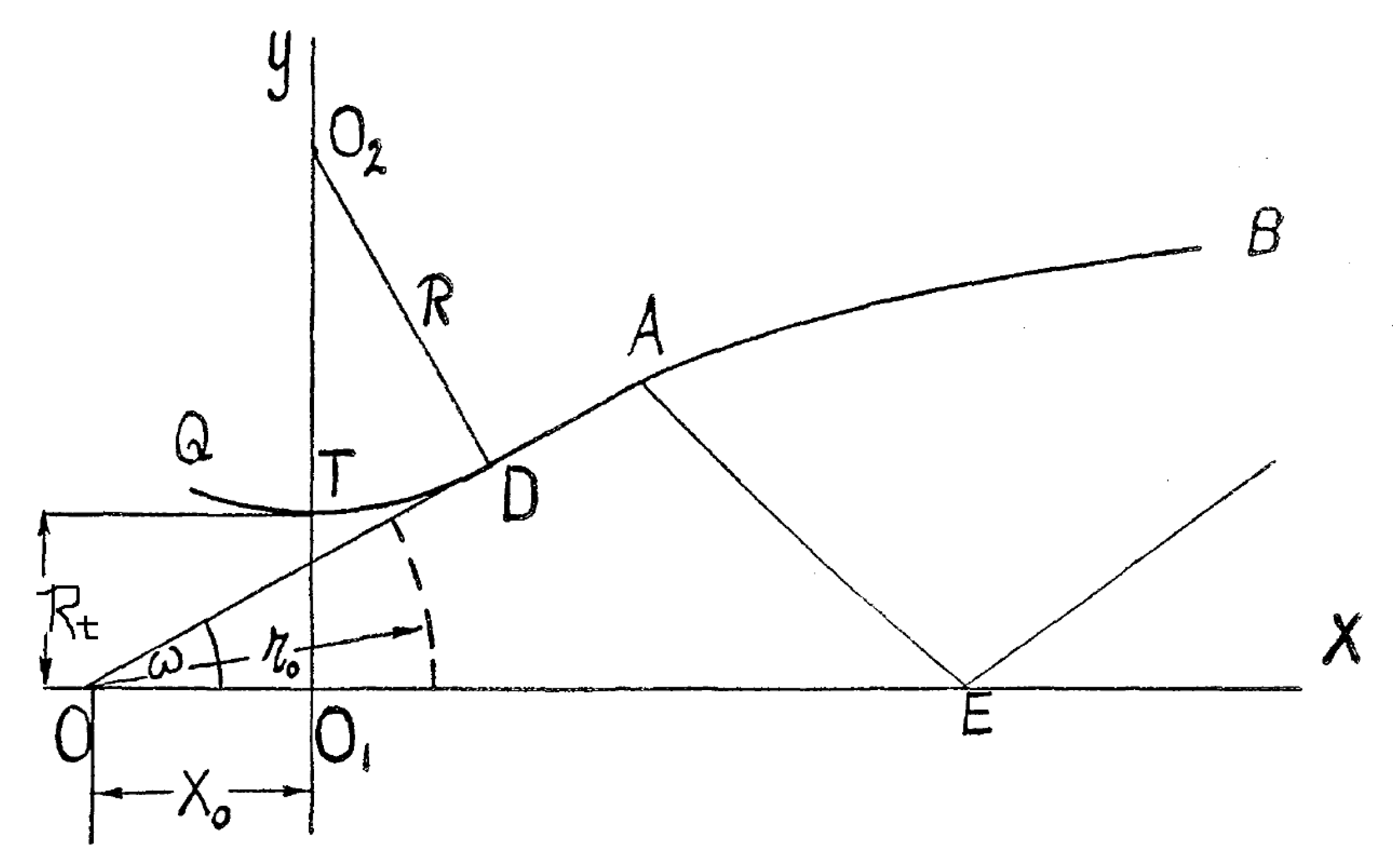
Figure 44.
Foelsch nozzle from in-house code for , and
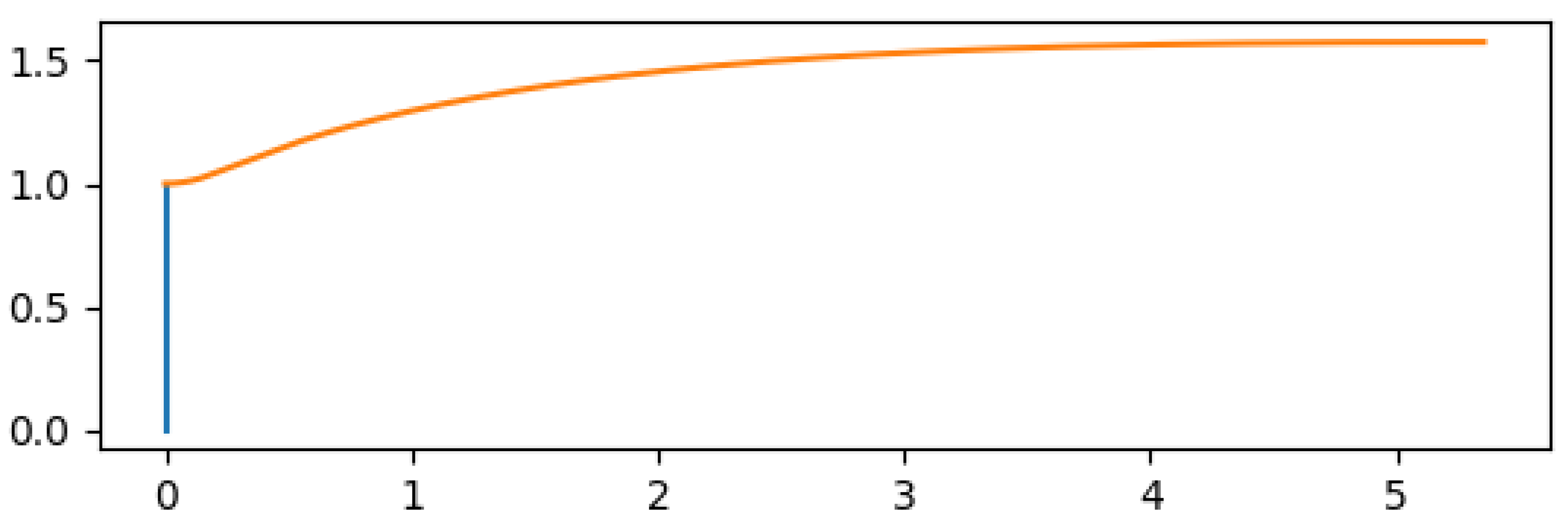
Figure 45.
Foelsch nozzle from in-house code for , and
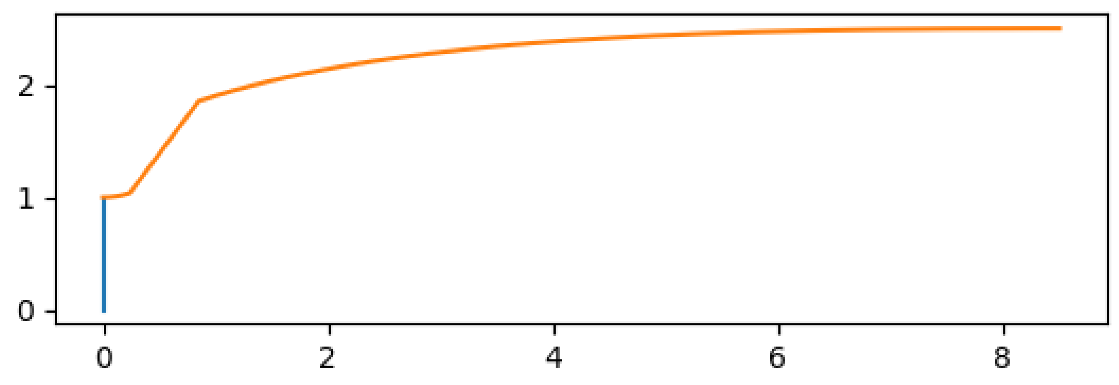
Figure 46.
Foelsch nozzle from in-house code for , and with smooth initial curve
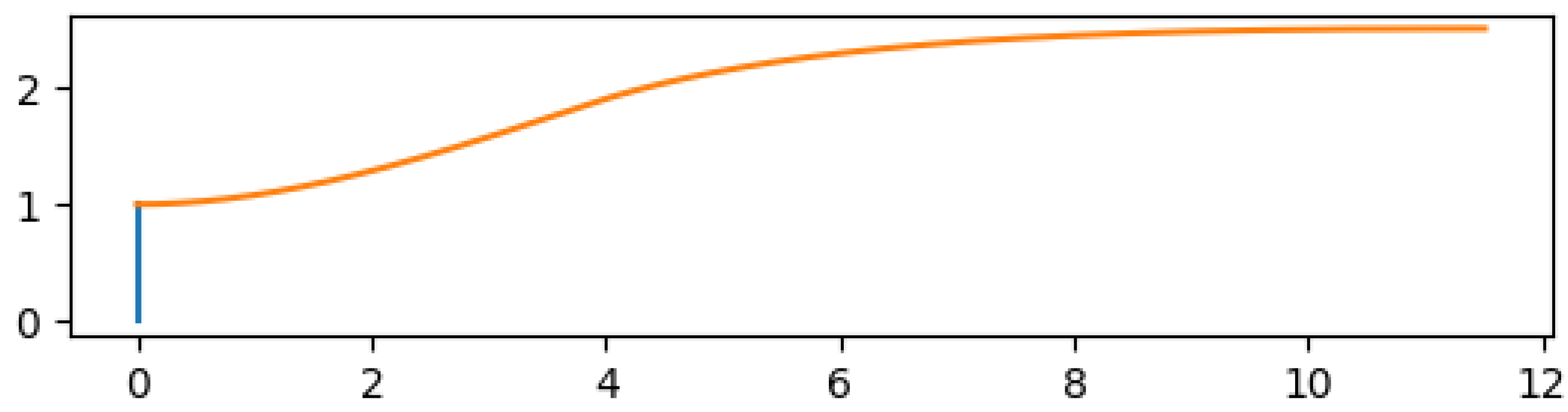
Figure 47.
Sivells nozzle scheme [46]
Figure 47.
Sivells nozzle scheme [46]
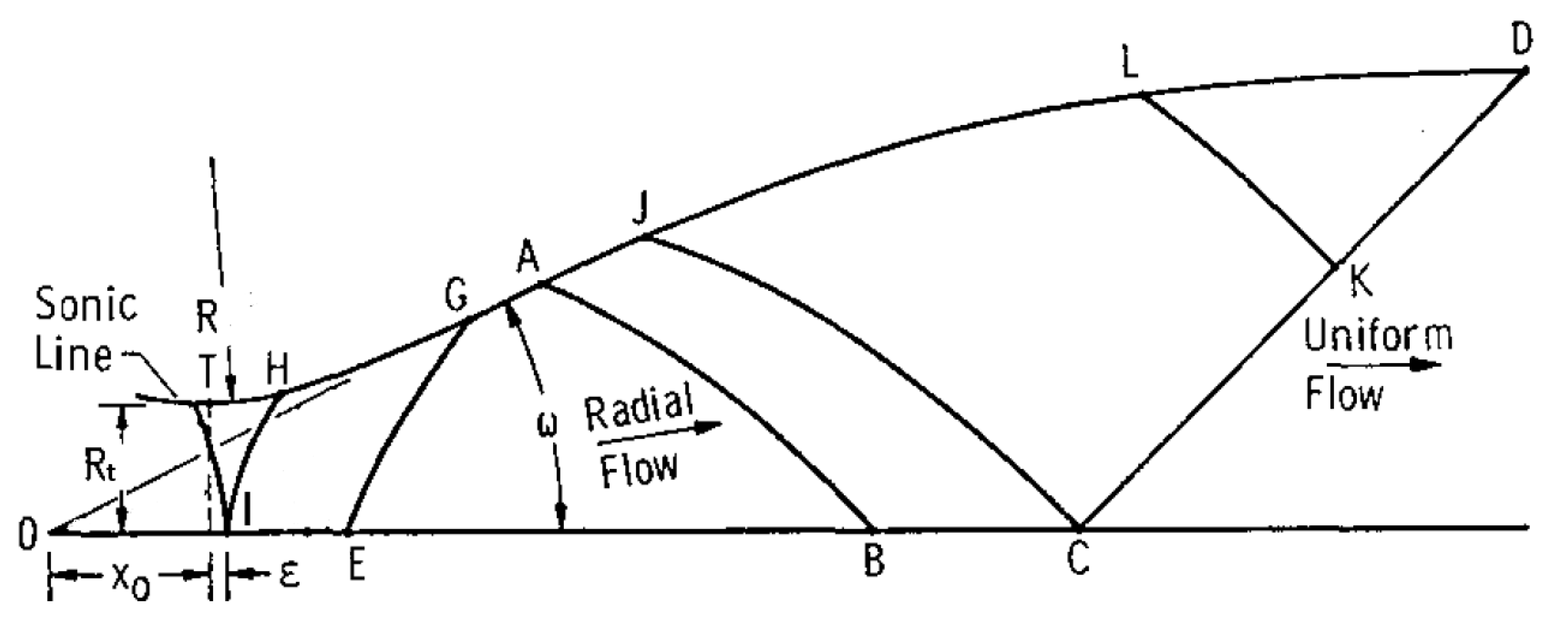
Figure 48.
Inviscid Sivells nozzle contour from CONTUR with
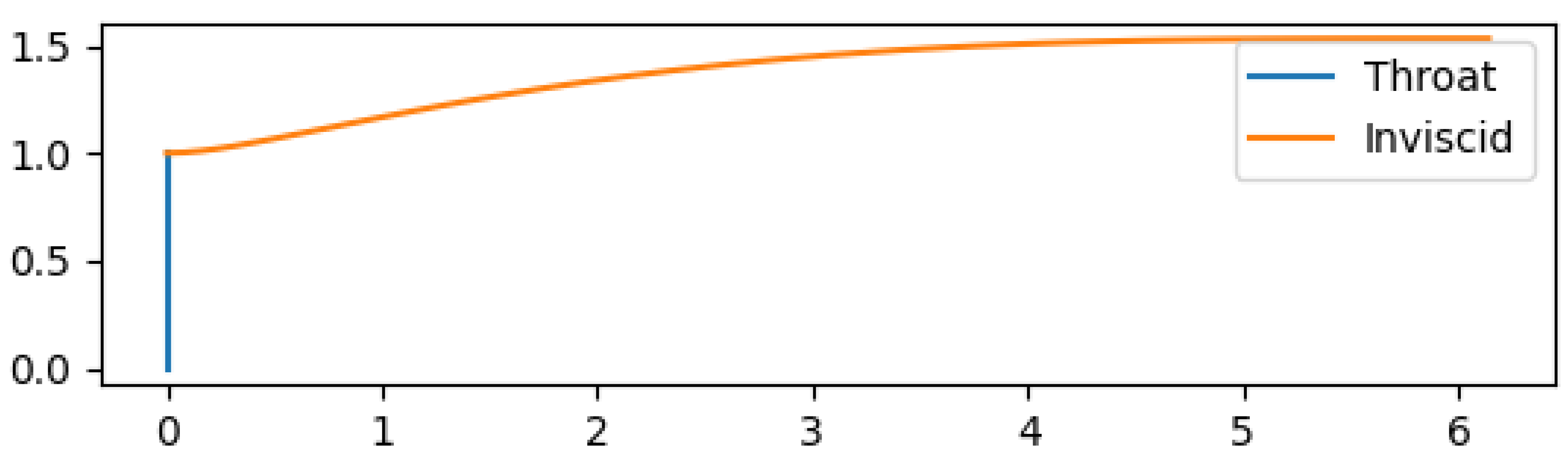
Figure 49.
Inviscid and Boundary-Layer corrected Sivells nozzle contour from CONTUR with
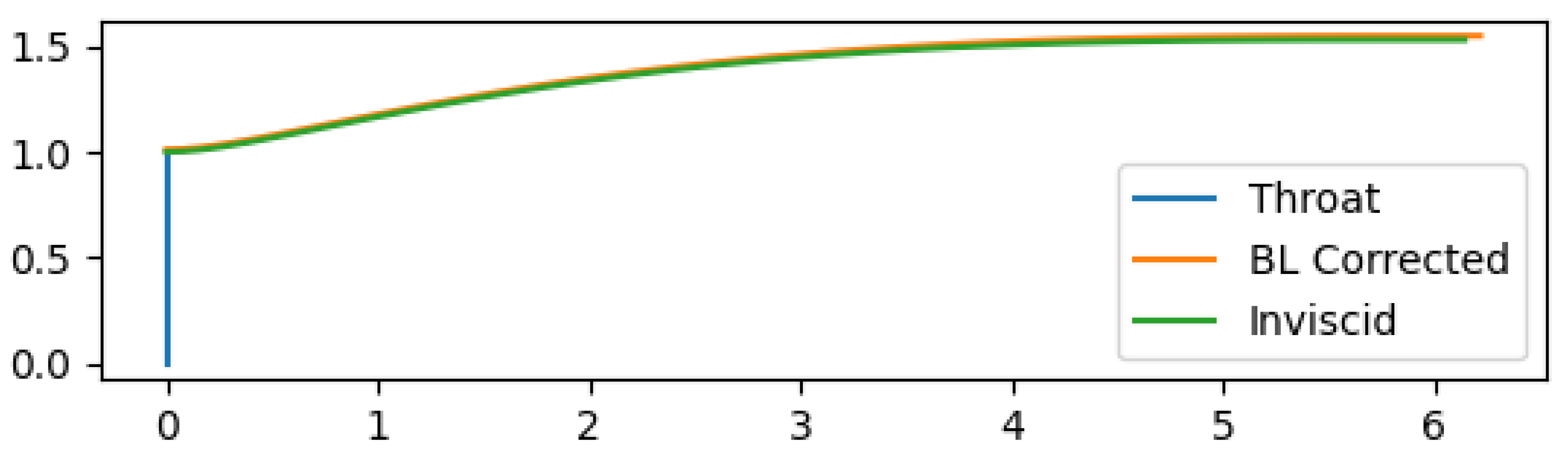
Figure 50.
Flow phenomena at an aerospike nozzle at: a) sea-level or low PR b) design altitude/PR and c) vacuum or high PR operations [49]
Figure 50.
Flow phenomena at an aerospike nozzle at: a) sea-level or low PR b) design altitude/PR and c) vacuum or high PR operations [49]
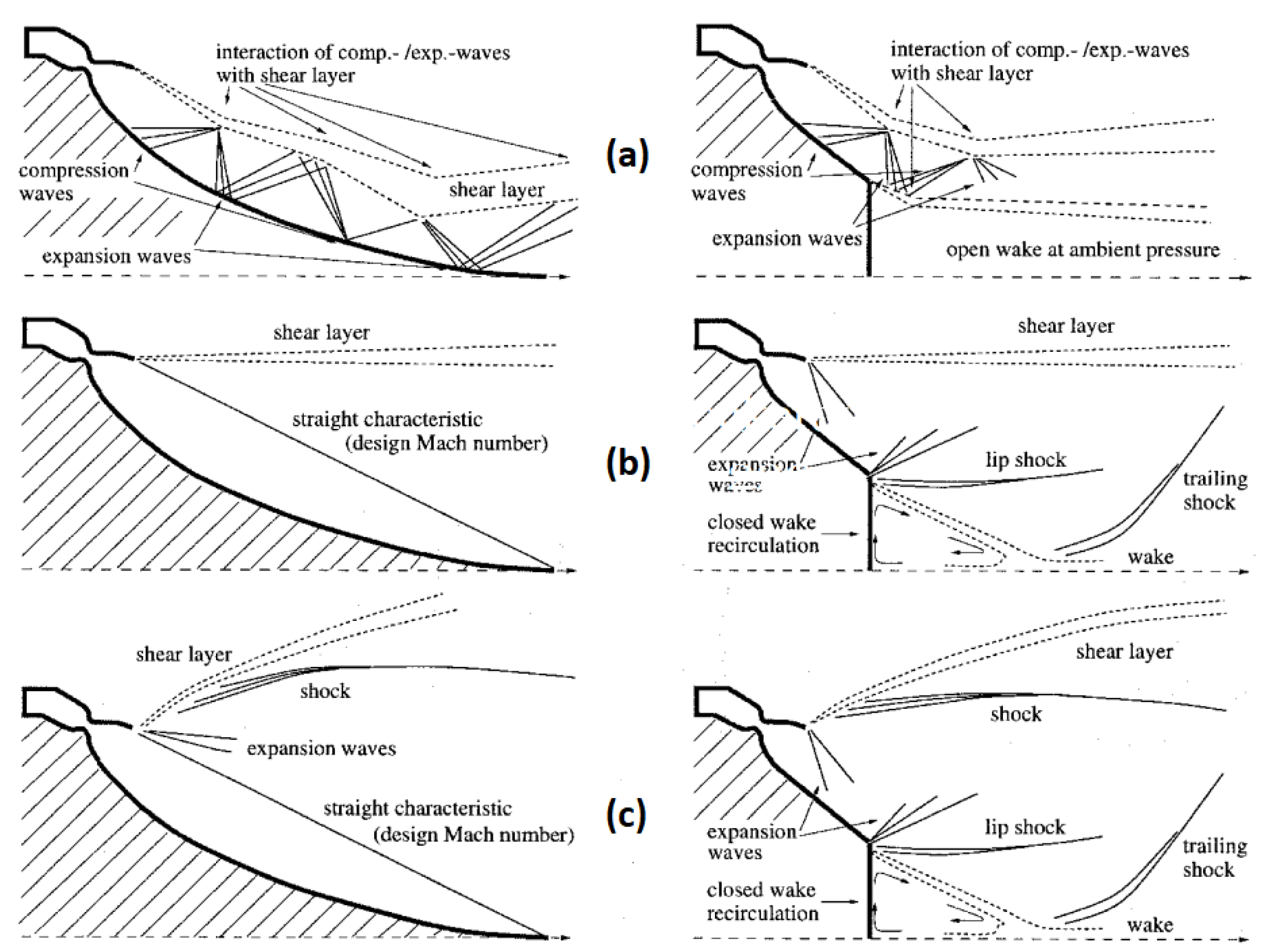
Figure 51.
Sketch of the centered expansion fan of an aerospike
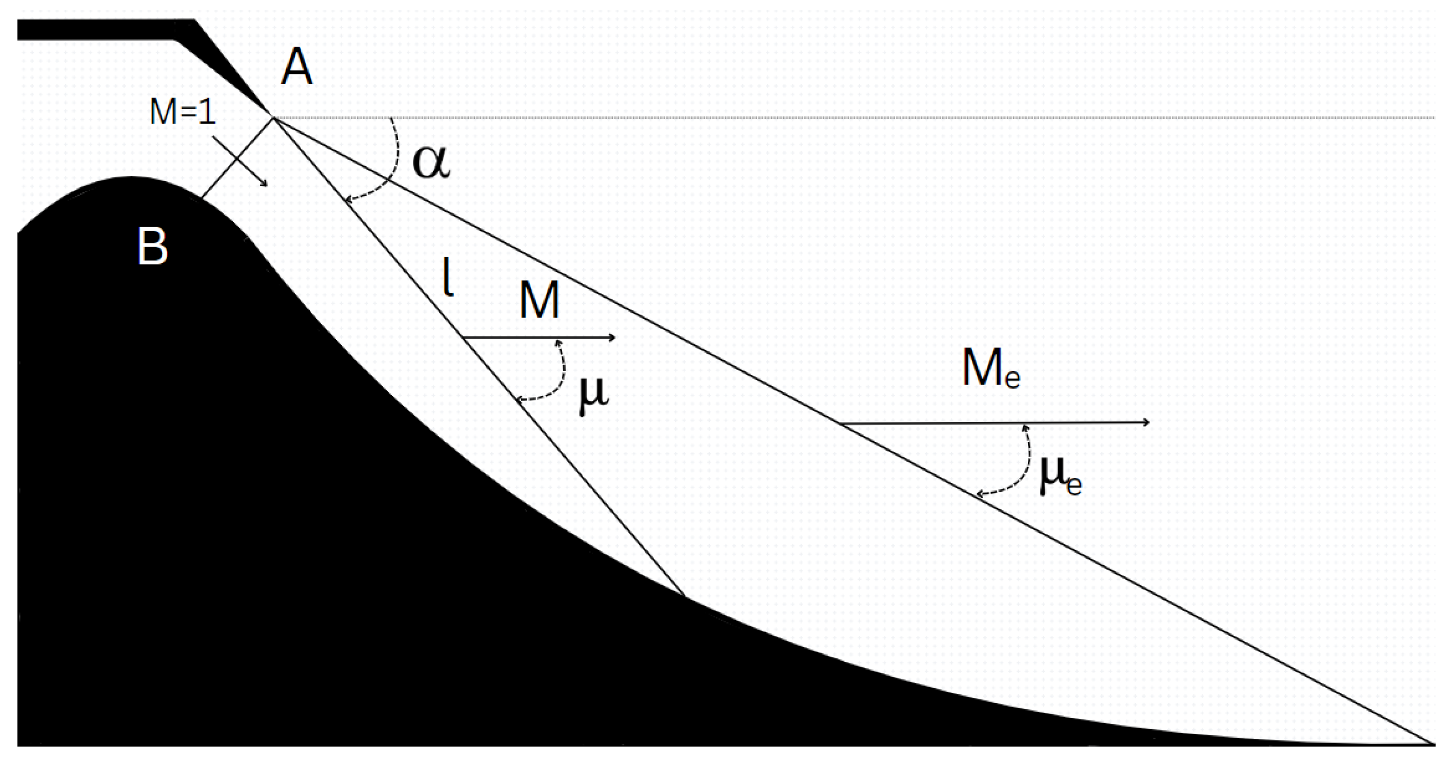
Figure 52.
Comparison of approximate and exact solutions in linear aerospike nozzle design [55]
Figure 52.
Comparison of approximate and exact solutions in linear aerospike nozzle design [55]
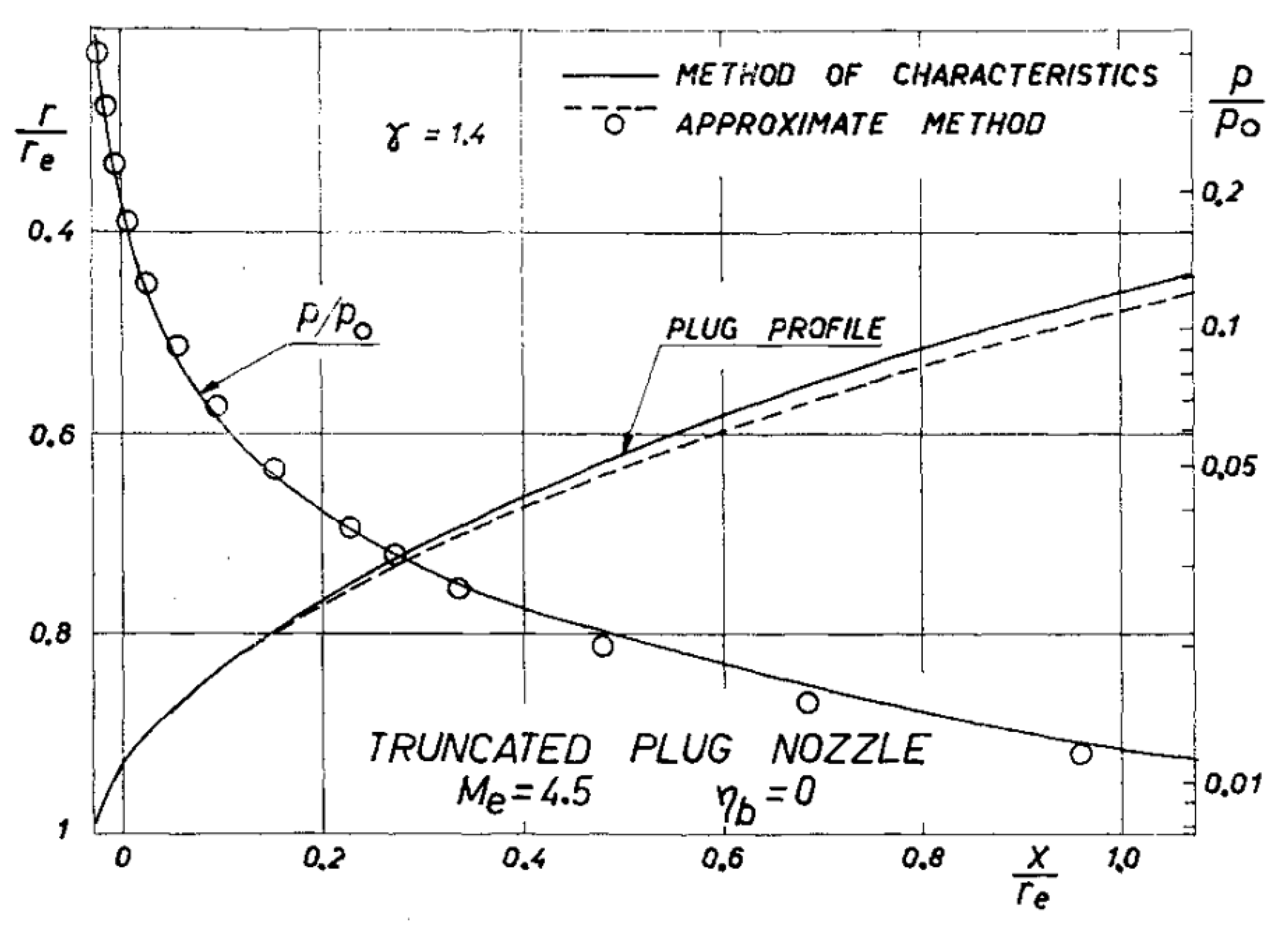
Figure 53.
Aerospike contour designed with Angelino’s method of in-house code
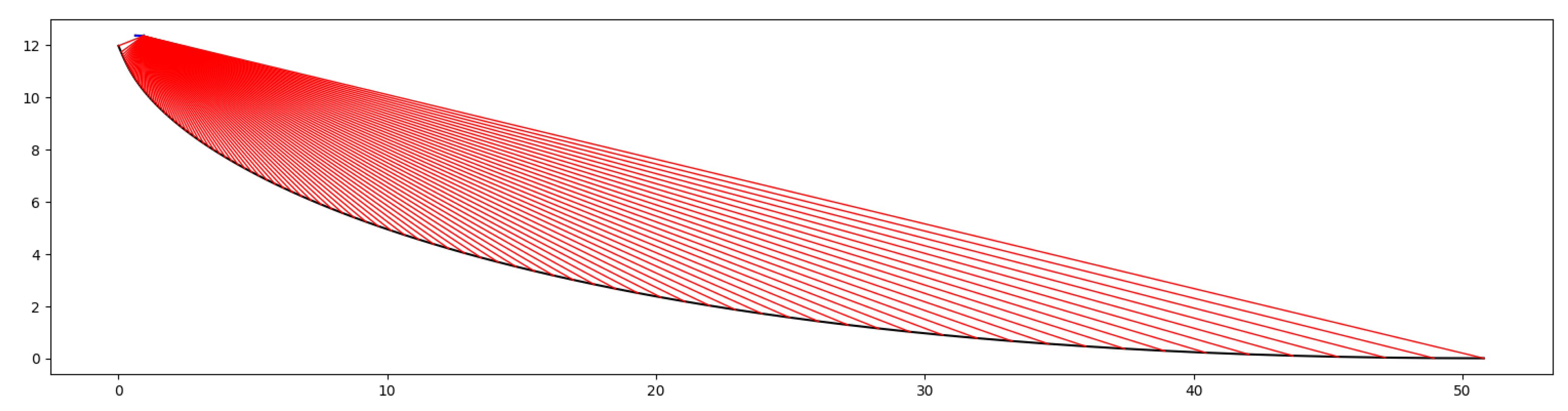
Figure 54.
Aerospike’s contour from Reference [60]
Figure 54.
Aerospike’s contour from Reference [60]
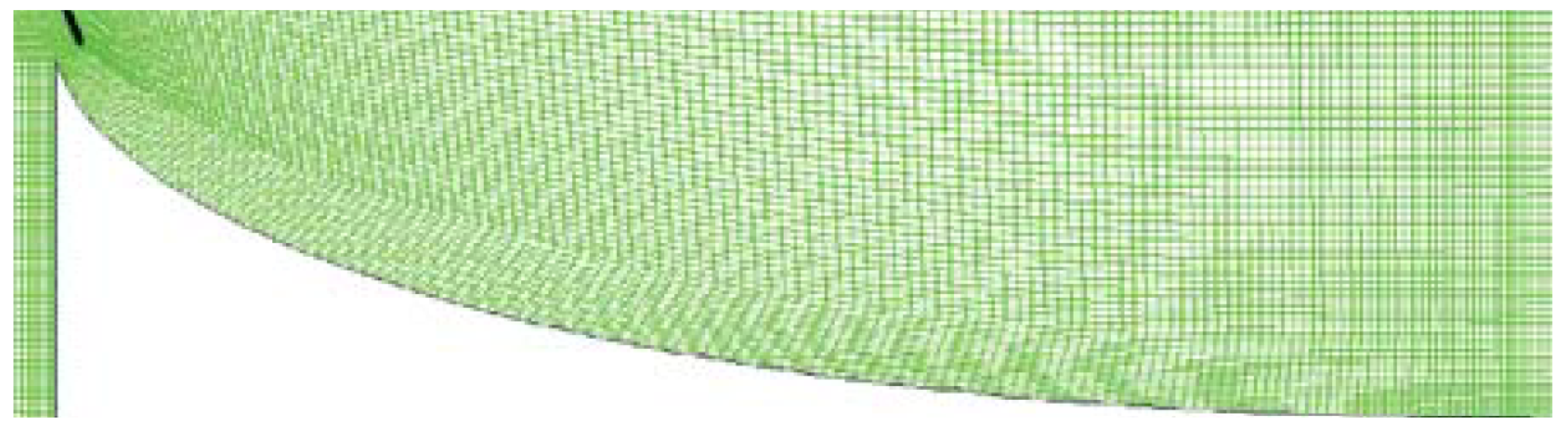
Figure 55.
Depiction of a Dual Bell nozzle [71]
Figure 55.
Depiction of a Dual Bell nozzle [71]
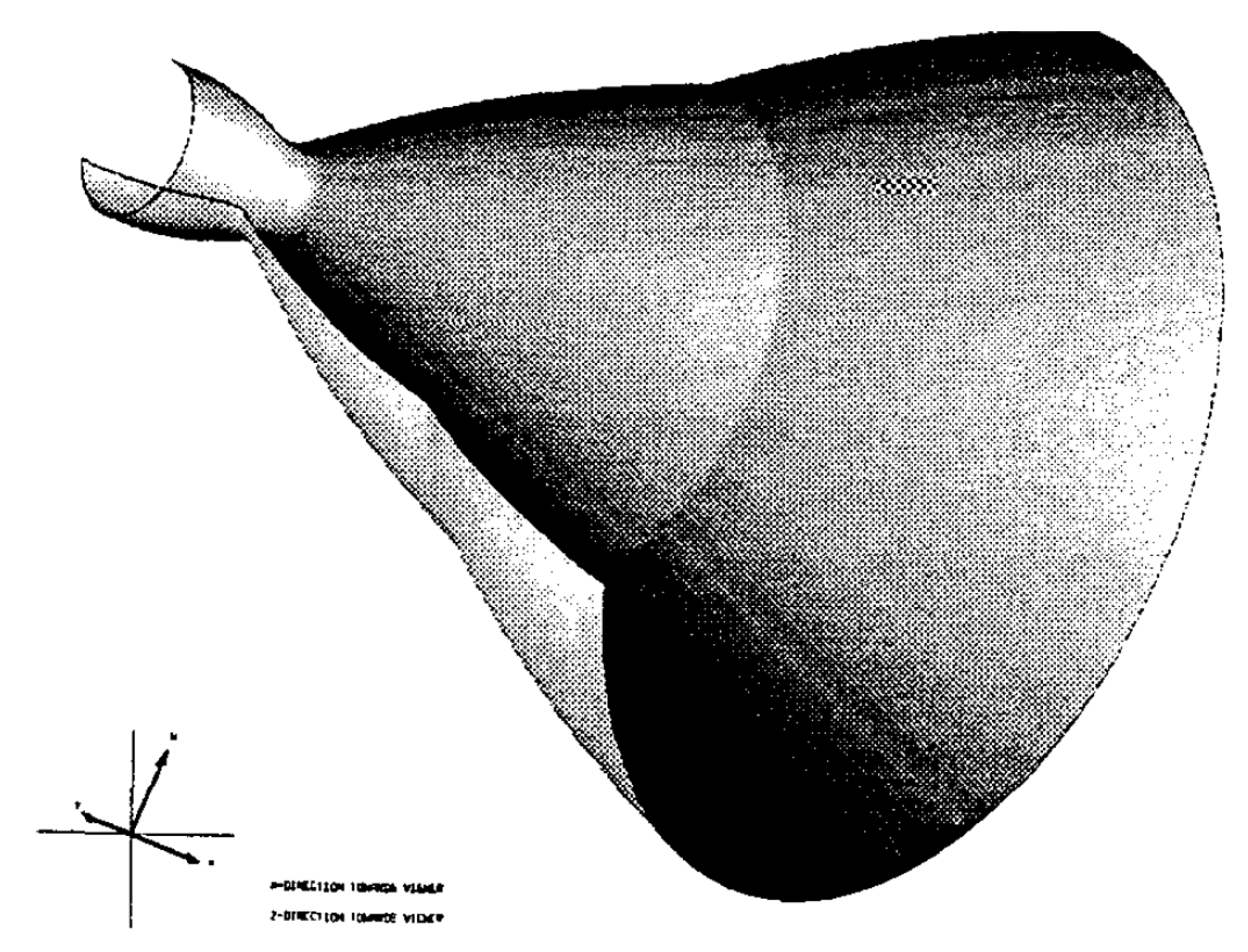
Figure 56.
Specific Impulse of Dual Bell nozzle vs Altitude [71]
Figure 56.
Specific Impulse of Dual Bell nozzle vs Altitude [71]
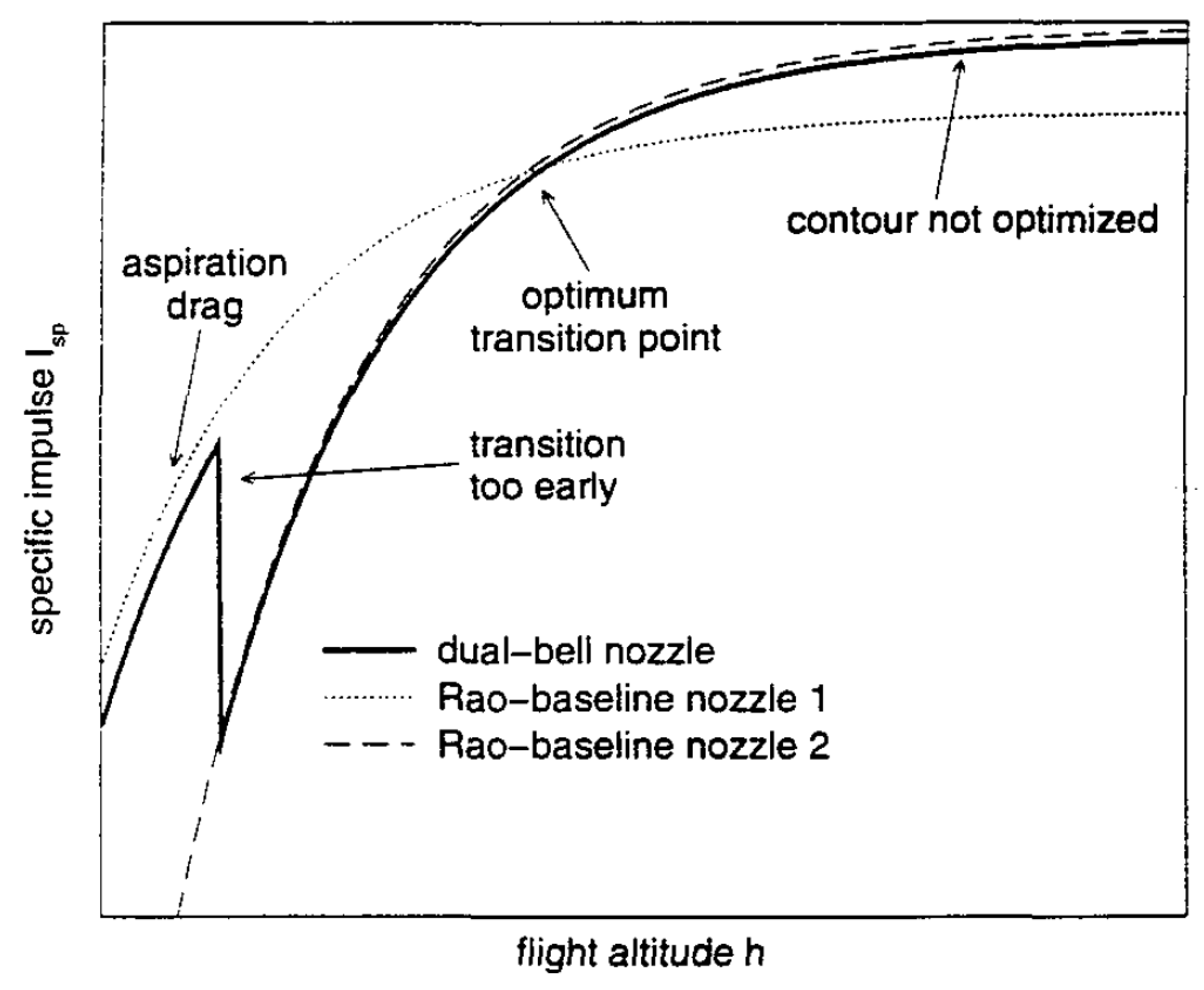
Figure 57.
Scheme of the Flow inside of a Dual Bell nozzle [49]
Figure 57.
Scheme of the Flow inside of a Dual Bell nozzle [49]
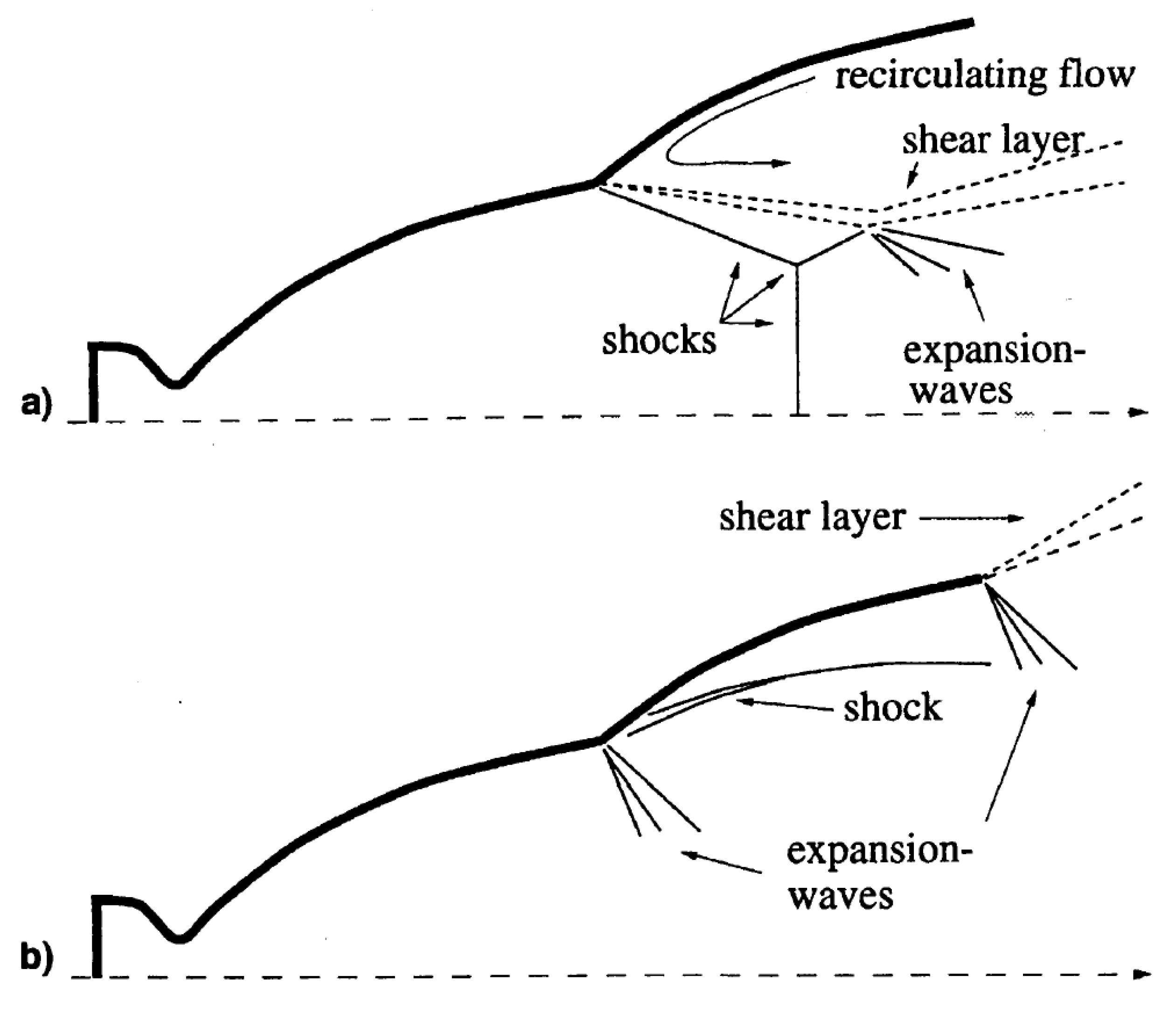
Figure 58.
Dual Bell nozzle contour from in-house code
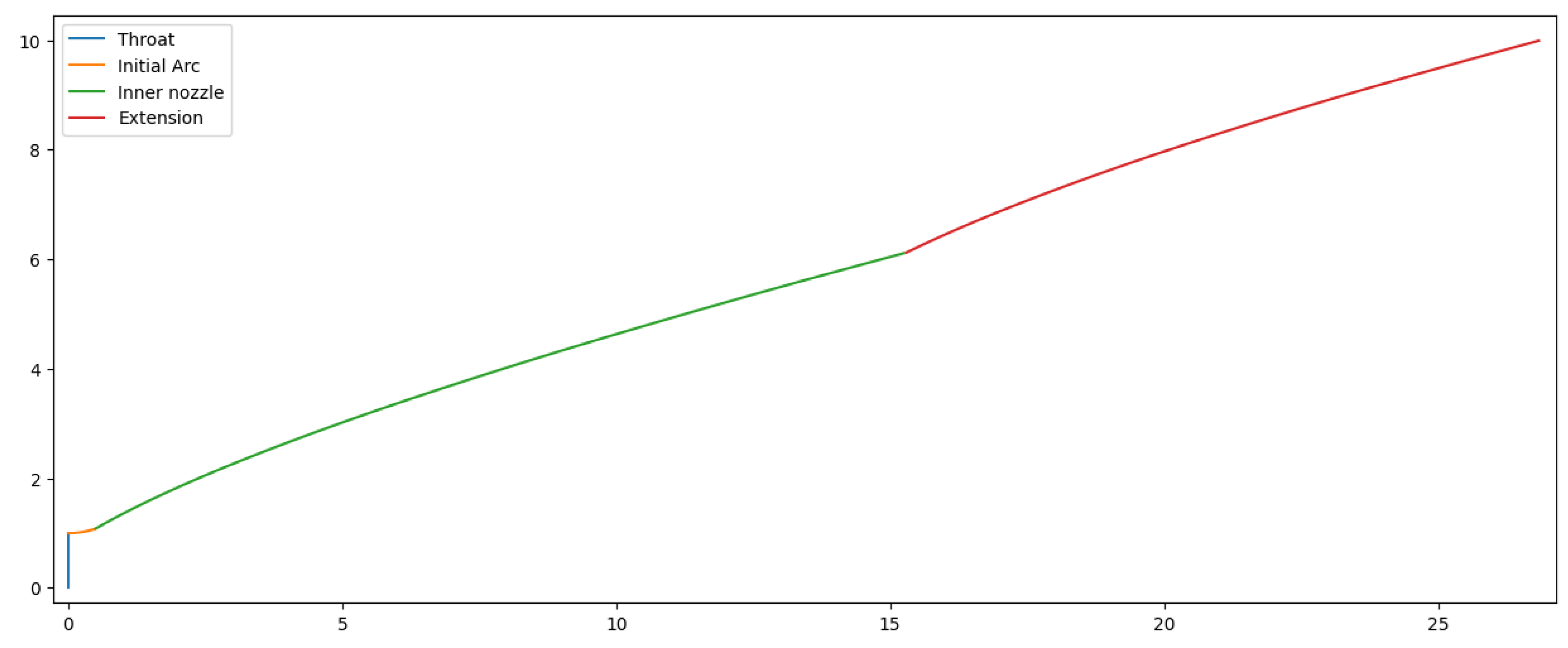
Figure 59.
Depiction of an E-D nozzle[49]
Figure 59.
Depiction of an E-D nozzle[49]
Figure 60.
Flow phenomena inside an E-D nozzle at: a) sea-level operation (open wake) and b) vacuum operation (close wake) [49]
Figure 60.
Flow phenomena inside an E-D nozzle at: a) sea-level operation (open wake) and b) vacuum operation (close wake) [49]
Figure 61.
MNG sketch [85]
Figure 61.
MNG sketch [85]
Figure 62.
Extendable nozzle sketch at: a) sea-level and b) vacuum operations [49]
Figure 62.
Extendable nozzle sketch at: a) sea-level and b) vacuum operations [49]
Figure 63.
Dual-throat nozzle sketch [49]
Figure 63.
Dual-throat nozzle sketch [49]
Figure 64.
Flow phenomena inside a dual-throat nozzle at: a) sea-level and b) vacuum operations [49]
Figure 64.
Flow phenomena inside a dual-throat nozzle at: a) sea-level and b) vacuum operations [49]
Figure 65.
Flow phenomena inside a dual-expander nozzle at: a) sea-level and b) vacuum operations [49]
Figure 65.
Flow phenomena inside a dual-expander nozzle at: a) sea-level and b) vacuum operations [49]
Table 1.
Standard Case for TOP performance Studies using MOC
| Standard Case | ||||||||
|---|---|---|---|---|---|---|---|---|
| Radius |
(º) |
(º) |
f |
(MPa) |
(K) |
Nodes Initial Line |
||
| 2.4 | 1.4 | 0.625 | 30 | 15 | 0.8 | 1 | 1200 | 200 |
Table 2.
TOP design parameters from equivalent TIC nozzle
| TIC Case | ||||||||
|---|---|---|---|---|---|---|---|---|
| Radius |
(º) |
(º) |
f |
(MPa) |
(K) |
Nodes Initial Line |
||
| 3.58 | 1.4 | 0.625 | 43.84 | 26.87 | 0.95 | 1 | 1200 | 200 |
Table 3.
TOP design parameters from equivalent TIC nozzle
| Nozzle Contour |
(s) |
of Quasi-1D Conical Nozzle |
(º) |
|||
|---|---|---|---|---|---|---|
| TIC | 639.338 | 99.11% | 3.531 | 3.375 | 3.823 | 28.546 |
| TOP | 650.835 | 100.89% | 3.556 | 3.317 | 3.700 | 27.520 |
Table 4.
Outputs from the Python code
| Output (for a 4.005 mm throat gap) | |
| Throat Angle () | |
| Pressure Ratio (PR) | 187.52 |
| Heigh (H) | 49.46 mm |
| Length (L) | 203.45 mm |
Disclaimer/Publisher’s Note: The statements, opinions and data contained in all publications are solely those of the individual author(s) and contributor(s) and not of MDPI and/or the editor(s). MDPI and/or the editor(s) disclaim responsibility for any injury to people or property resulting from any ideas, methods, instructions or products referred to in the content. |
© 2025 by the authors. Licensee MDPI, Basel, Switzerland. This article is an open access article distributed under the terms and conditions of the Creative Commons Attribution (CC BY) license (http://creativecommons.org/licenses/by/4.0/).
Copyright: This open access article is published under a Creative Commons CC BY 4.0 license, which permit the free download, distribution, and reuse, provided that the author and preprint are cited in any reuse.


