
Submitted:
20 March 2025
Posted:
21 March 2025
You are already at the latest version
Abstract
This study introduces a novel state estimation framework that incorporates Deep Neural Networks (DNNs) into Moving Horizon Estimation (MHE), shifting from traditional physics-based models to rapidly developed data-driven techniques. A DNN model with Long Short-Term Memory (LSTM) nodes is trained on synthetic data generated by a high-fidelity thermal model of a Permanent Magnet Synchronous Machine (PMSM), which undergoes thermal derating as part of the torque control strategy in a battery electric vehicle. The MHE is constructed by integrating the trained DNN with a simplified driving dynamics model in a discrete-time formulation, incorporating the LSTM hidden and cell states in the state vector to retain system dynamics. The resulting optimal control problem (OCP) is formulated as a nonlinear program (NLP) and implemented using the \texttt{acados} framework. Model-in-the-loop (MiL) simulations demonstrate accurate temperature estimation, even under noisy sensor conditions or failures. Achieving threefold real-time capability on embedded hardware confirms the feasibility of the approach for practical deployment. The primary focus of this study is to assess the feasibility of the MHE framework using a DNN-based plant model instead of focusing on quantitative comparisons of vehicle performance. Overall, this research highlights the potential of DNN-based MHE for real-time, safety-critical applications by combining the strengths of model-based and data-driven methods.
Keywords:
state estimation
; deep learning
; moving horizon estimation
; nonlinear and optimal automotive control
; neural networks
; temperature control
; electric machine
1. Introduction & Background
State estimation has been a critical area of research for several decades, playing a fundamental role in various engineering disciplines by providing robust and reliable feedback for control systems [1]. The mathematical foundations of state estimation can be traced back to Carl Gauss in the early 1800s, with further advancements in the 20th century, including Maximum Likelihood Estimation [2] and Linear Minimum Mean-Square Estimation [3]. However, the applicability of these early formulations to real-time systems was limited by available computational resources. The introduction of dynamic state estimation techniques, such as the Kalman Filter and the Luenberger Observer, revolutionized the field by enabling online estimation based on system dynamics and measurement uncertainty [4]. As the focus of both academia and industry moved to non-linear systems, extensions such as the Extended Kalman Filter (EKF) and Unscented Kalman Filter (UKF) were developed to address non-linearities in state estimation [5,6]. More recently, research has focused on state estimation techniques that can incorporate constraints on states and parameters, like Moving Horizon Estimation (MHE) [7].
The main idea of MHE is to compute a state estimate x by solving an optimization problem over a finite time horizon. At each sample time as soon as a measurement y is made available the horizon is shifted ahead in time in a receding horizon fashion and a new estimate is calculated. Figure 1 illustrates the MHE’s operating principle using the receding horizon.
Compared to Kalman-based approaches, MHE offers improved handling of constraints, disturbances, and system non-linearities, making it a powerful tool for advanced estimation tasks [8].
A critical aspect of modern state estimation is data assimilation, which integrates sensor measurements with dynamic process models to improve the accuracy of the estimation [9]. Traditional approaches rely on physics-based models, which require detailed system knowledge and intricate mathematical formulations. However, as systems become increasingly complex, the development of precise mathematical models becomes a challenge. Besides, accurate models might be computationally too expensive in particular for real-time applications [10]. These models often involve high-dimensional equations that demand significant computational resources, making them less practical for embedded control systems with stringent latency constraints. To address these challenges, data-driven approaches such as system identification, machine learning, and deep learning have gained prominence [11].
Deep learning architectures, inspired by biological neural networks, progressively build representations of input data while minimizing the need for manual feature engineering [12,13]. The layers in a Deep Neural Network (DNN) consist of neurons that integrate weighted inputs via activation functions. This function introduces non-linearity that is essential for learning complex tasks. While the basic calculations within the neurons remain consistent, the arrangement of the neurons play a crucial role in how the information is processed giving rise to various neural network architectures. Among these, Recurrent Neural Networks (RNNs) are particularly suited for dynamic systems due to their ability to retain temporal information [14]. Long Short-Term Memory (LSTM) networks, a variant of RNNs, are especially effective for time-series modeling, as they mitigate vanishing gradient issues and capture long-term dependencies [15].
The rapid advancement of DNNs has enabled the modeling of complex non-linear relationships without explicit system equations, making them invaluable for state estimation in systems where deriving accurate mathematical models is challenging. DNN-based models provide a scalable alternative by learning system behaviour directly from data, eliminating the need for complex physics-based formulations and enabling efficient real-time deployment. Several studies have successfully integrated DNNs into state estimation frameworks, with applications in pseudo-measurement generation, parameterized EKF formulations, and RNN-based non-linear system identification [16,17,18]. Notably, the use of LSTM and DNN-based models has also been explored in control applications in previous works, such as model predictive control (MPC) for combustion engines [19], and rapid development toolchains for a low temperature combustion process [20]. However, DNN-based MHE for state estimation remains unexplored. This research addresses that gap by leveraging LSTM-based models to enhance adaptability and robustness in state estimation.
The novelty of this research lies in developing a MHE that integrates a DNN-based plant model — specifically using LSTM architecture — in place of a white- or grey-box model, aiming to improve estimation accuracy while reducing modeling effort and computational complexity.
Building on prior work by [21] that introduced a DNN-based Model Predictive Controller (MPC) for thermal torque derating of a Permanent Magnet Synchronous Machine (PMSM) in a Battery Electric Vehicle (BEV), this research extends the work by integrating a DNN-based state estimator [21,22]. Thermal derating is a protective strategy that limits the torque output of an electric machine to prevent overheating and ensure long-term reliability. The previous study focused on optimizing torque commands while ensuring temperature constraints of the PMSM, using a Model-in-the-Loop (MiL) simulation with a reference velocity trajectory from one lap of Nürburgring Nordschleife.
A high-fidelity 70-node Lumped Parameter Thermal Network (LPTN) model provided by DENSO, the PMSM’s manufacturer, has been experimentally validated on test benches and used to determine the motor temperature for feedback to the MPC within the plant. However, in real-world applications, temperature data obtained from sensors is often noisy and inaccurate, highlighting the necessity for robust state estimation. To validate the proposed approach, the DNN-based state estimator is integrated into the existing MiL simulation setup. The estimator processes noisy sensor measurements to reconstruct accurate system states, which are then provided to the MPC for real-time process control. The state estimator is formulated as a MHE problem and is implemented using the acados optimal control framework, ensuring compatibility with embedded systems.
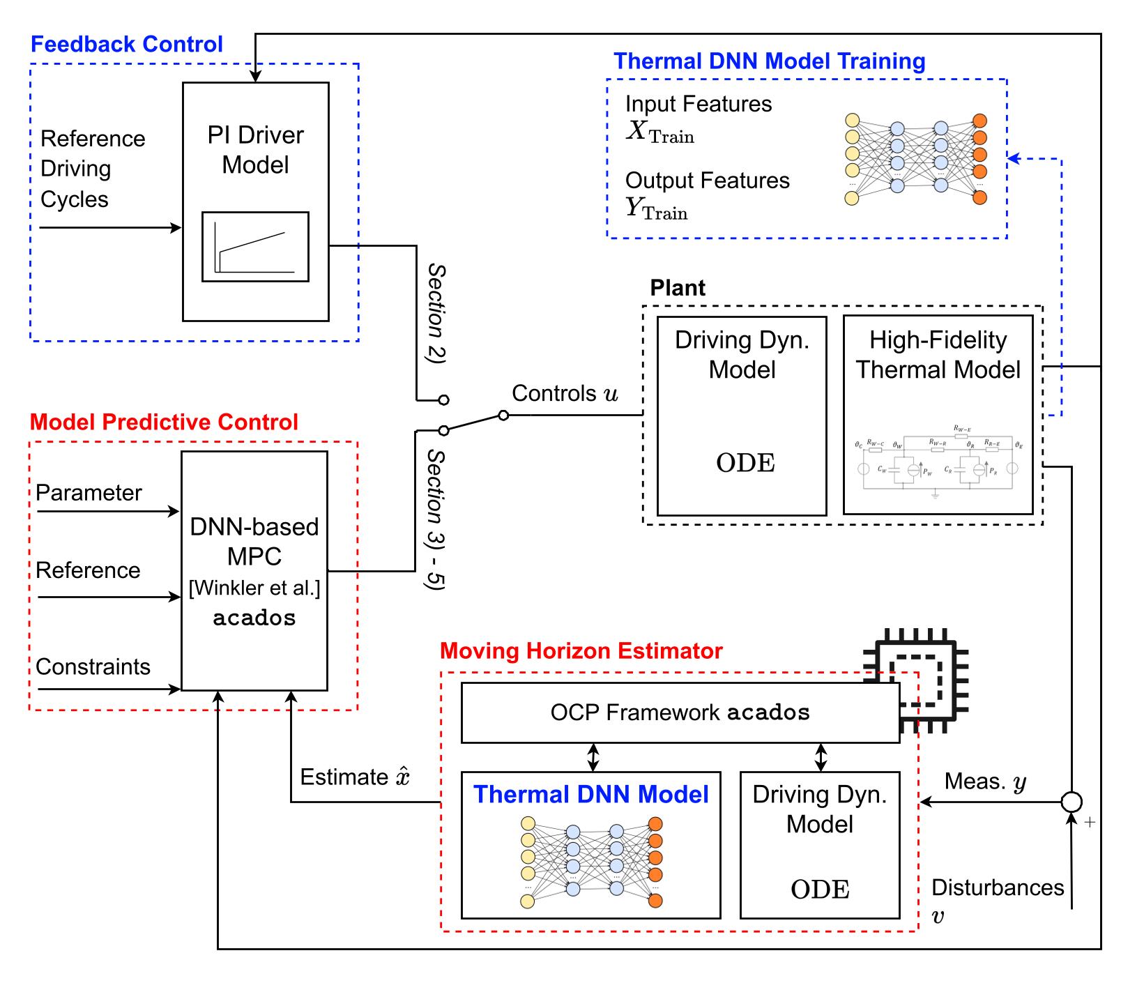
To provide a high-level understanding of the approach and methodology, the graphical abstract in Figure 2 illustrates the key components of the proposed MHE framework, including data generation, DNN training, and its simulative and embedded validation. The central objective of this research is to demonstrate the feasibility of a DNN-based MHE framework. Instead of focusing on quantitative comparisons of vehicle performance under MPC control, the study a qualitative evaluation — assessing how effectively the DNN-based MHE estimates temperature states and how robust it performs in the presence of injected sensor faults.
The paper is divided into the data generation process (Section 2), the MHE development (Section 3), and the subsequent simulative and embedded integration for validation (Section 4 and Section 5, respectively) as shown schematically in Figure 2.
This research makes the following key contributions:
- Integration of DNN with MHE: This work represents one of the first attempts to integrate a DNN-based model with MHE, providing a novel framework for state estimation.
- Deployment and validation on embedded systems: The feasibility of implementing a DNN-based MHE framework in real-time is demonstrated. This research is also one of the first to test and validate the deployment of DNN-based state estimation on real-time hardware using the acados optimal control framework [23].
The datasets and scripts presented in this work are publicly available [24].
2. Deep Neural Network Modeling
This chapter presents the development of the DNN model used for thermal state prediction. It covers the LSTM architecture, the experimental setup with synthetic data generation, and the training process of the network.
2.1. Long Short-Term Memory Network
LSTMs, one of the most popular variants of RNN, have the ability to maintain a form of memory, enabling them to influence current inputs and outputs based on past sequence information [14]. To regulate the flow of data, LSTMs introduce memory cells and gate units [15]. The core computational unit of the LSTM network is called the memory cell (or simply "cell"), and these networks were primarily designed for sequence modeling while addressing the vanishing gradient problem [14,25].
Each LSTM cell consists of three gates: the forget gate, the input gate and the output gate that regulate information flow using sigmoid () and hyperbolic tangent (tanh) activation functions to maintain stable outputs [14]. The following equations mathematically define the operations within an LSTM cell, where each gate contributes to memory updates and output generation:
where are the weighting matrices applied to the input vector . are weight matrices of the previous hidden state . In this equation, ⊙, is an element-wise multiplication and are the biases. is the input gate, is the forget gate, is the cell candidate, is the output gate, is the cell state, and is the hidden state. Two activation functions are used in Equation (1) which are given as:
- hyperbolic tangent activation function:
- sigmoid activation function:
These activation functions are used to introduce non-linearity into the otherwise linear layers. Figure 3 shows a visualization of the information flow depicted in Equation (1).
Due to the temporal dependencies in LSTMs, storing both the cell and hidden states across timesteps increases memory requirements.
2.2. Experimental Setup and Data Generation
The proposed state estimator, akin to the approach of previous works in [21] uses one-dimensional white-box driving dynamics and thermal black-box DNN dynamics to predict the thermal states of a PMSM and generate accurate and robust estimates [21,22]. The DNN, integrated with the state estimator, predicts the temperature gradients of the PMSM to calculate accurate thermal states of the system. For simplification, the PMSM is represented by two thermal masses () corresponding to measurable real-world temperatures at the test-bench of the windings and the rotor, respectively.
When combined with the MPC framework developed by [21], the resulting model-in-the-loop (MiL) simulation enables safe thermal derating of a BEV, by effectively handling noisy PMSM temperature measurements while ensuring compliance with thermal constraints.
The performance and accuracy of the DNN models heavily depend on the quality and quantity of training data. To efficiently generate the required data without relying on extensive test-bench experiments, a simulation framework is employed. Within this framework, a proportional-integral (PI) driver controller computes the torque requests to the Electric Machine (EM) and friction brake based on the vehicle velocity v. These include (), where the torque of the EM is split into acceleration and braking components: . A one-dimensional longitudinal model utilizes these torque values to calculate vehicle velocity utilizing the ordinary differential equation (ODE):
where kg is the vehicle mass (including the driver), is the drag coefficient, is the rolling friction coefficient, m is the dynamic tire radius, and is the car’s cross sectional area. The transmission ratio is given by , while the maximum vehicle speed is km/h. depicts an external parameter and input as the road inclination defined by the driving cycle, while and g are the air density and gravitational acceleration, respectively. In this study, a typical minicar BEV is used and its parameters have been validated in previous works by [22].
The relation between the vehicle speed v in Equation (4) and the rotational speed of the electric machine is as follows: . Thus, the primary operating point of the EM, the torque and the rotational speed serve as the primary inputs to the high-fidelity LPTN model, determining the rotor and winding temperature () of the machine, with their derivatives ) being monitored as well. The 70-node high-fidelity LPTN model is provided by the PMSM’s manufacturer DENSO and its parameters have been fitted using extensive experimental test-bench data. The full simulation model, implemented in MATLAB/Simulink is depicted in Figure 4 and operates at a sample rate of .
A driving cycle serves as the primary predefined input for the data generation model, providing the reference velocity for the PI controller and the respective road inclination . To achieve higher and thus safety critical PMSM temperatures, the WLTP Class 3 driving cycle is customized, deliberately influencing the data diatribution. Figure 5 illustrates the velocity profile of the customized cycle and the corresponding temperature response, where only the winding temperature is shown, as the rotor temperature remains below critical levels and is therefore omitted. The figure also highlights that a significant portion of the data lies within the safety-critical temperature range of the machine, between 150 °C. and 160 °C, where permanent damage can occur.
2.3. Neural Network Training
The network architecture comprises four layers: the input, LSTM, Fully Connected (FC), and output layer. The LSTM layer consists of 8 LSTM cells that compute the temporal dependencies between the inputs. Figure 6 shows the architecture of the DNN used for training.
Drawing inspiration from LPTNs and the physical intuition behind heat transfer, this work models temperature evolution by predicting temperature change rates rather than absolute temperatures. Subsequently, the input features to the DNN are rotational speed of the EM , torque of the EM , winding temperature and rotor temperature of the EM. The DNN’s output features are the gradients and , at timestep k. This can be summarized as follows in Equation (5):
The depth of a DNN directly influences computational complexity, as each additional layer increases the number of learnable parameters and matrix operations. To ensure real-time feasibility, particularly for integration with optimization techniques like MPC and MHE, the DNN’s depth and the number of recurrent nodes are constrained. The training data distribution is shown in Figure 7 for the two outputs and .
The training is performed with the training hyperparameters as referenced in Table 1.
The resulting loss-epoch plot of the training is shown in Figure 8, while the prediction results of the final network on the unseen test dataset are depicted in Figure 9. The unseen test dataset consists of data for a simulated lap on the Nürburgring Nordschleife with its high power requirements, thus posing a major challenge to the electric drivetrain and its thermal constraints. To solve the trade-off between the DNN’s depth and thus the computational complexity and the DNN’s prediction performance, empirical studies are performed, which are omitted here for brevity. The results in Figure 9 show a good correspondence with the ground truth from the high fidelity model, achieving an RMSE of 0.0373 (degC/s) and 0.0282 (degC/s) and an NRMSE of 2.77% and 9.39% for and , respectively. Further performance metrics are depicted in Table 2.
The lower accuracy in predicting can be attributed to the complexity of the high-fidelity thermal model and the weaker influence of the selected features. To be more precise, the network struggles with lower rotor temperatures due to a lack of training data in that range (see Figure 7). However, since the focus of data generation was on higher, critical temperatures, this limitation is acceptable, and the network is considered sufficiently accurate due to its superior performance on .
The presentation of the DNN predictions in the time-domain of the unseen test dataset of the Nürburgring Nordschleife in Figure 10 underlines the good performance of the chosen network.
Since the neural network predicts temperature gradients, explicit first-order Euler integration with an initial temperature of = 60 °C for both the winding and the rotor is used to visualize the absolute temperatures.
3. Estimator Formulation
MHE is employed to reconstruct system states by solving an optimization problem at each timestep. The optimization problem has a similar structure as an Optimal Control Problem (OCP) such that tailored solvers for OCP-structured problems can be used. Following successful training of the DNN model, the next step involves formulating the estimator and implementing it within the OCP-structure of the acados framework. Thereto, both the driving dynamics and the DNN-based thermal model are reformulated in a discrete-time, optimization-compatible form.
3.1. MHE Problem Formulation
The dynamics depicted here are based on a discrete-time, non-linear, time-invariant system [26]:
with state , measurement , process disturbance , measurement disturbance . The non-linear function describing the system dynamics and the measurement model are now developed, bringing the DNN-based thermal model and the one-dimensional driving dynamics model in a common, discrete form.
Firstly, the driving dynamics in Equation (4) can be further summarized and discretized using explicit Euler integration of first order with integration interval as:
with summarizing the driving dynamics equation.
Equation (1) presents the equations for an LSTM unit. This formulation is transformed into a forward propagating process model by representing operations as equations incorporating stored weights and biases. The LSTM internal memory states - the hidden and cell states - are included in the network inputs and outputs due to the unrolling of the recurrent layer. Adding the FC layer of the DNN provides the full dynamics representation of the DNN:
The function thus summarizes the complete DNN dynamics.
Finally, the absolute temperature predictions for the next timestep using explicit first-order Euler integration are defined as:
Following the dynamics from Equation (7) and Equation (9), the functions within the MHE dynamics in Equation (6) can be further defined as:
Furthermore, using these dynamics, the MHE optimization problem including the objective function is defined as:
Here, represents the optimization variables, while forms the measurement window. The weighting matrices Q and R are positive definite diagonal matrices corresponding to process and measurement variances; is the weighting matrix of the arrival cost. MHE operates by optimizing on a fixed horizon of N past measurements , where past information outside the estimation window is not directly included in the optimization (see also Fig Figure 1). The arrival cost, , addresses this by approximately incorporating information from prior states .
This concludes the formulation of the MHE and sets the stage for the implementation into an OCP-structured NLP in the framework acados in the following subsection.
3.2. Implementation in acados
State Estimation is performed by minimizing the variance between system predictions and measurements. To solve the MHE optimization problem, the optimal value of the additive process noise w must be determined to yield the most accurate estimate. The noise w is thus treated explicitly as an optimization variable.
This leads to the optimization problem to be formulated as an OCP, where the process noise w is considered as the controls input. Here, the OCP is structured around four sets of variables: states x, controls u, parameters p, and measurements y, each of which is defined below.
The primary states to be estimated include the winding and rotor temperatures (), with state evolution governed by the DNN-based thermal model.Given the recurrent nature of an RNN, its hidden and cell states are incorporated into the state vector, resulting in an increased state dimension that depends on the number of LSTM units (here: 8):
With the process noise defined as an additive term, the state evolution as seen in Equation (10) can be stated as:
Further, the control vector can be represented as:
The process noise follows a Gaussian distribution with a variance , a diagonal matrix derived from the variance of the states. This variance matrix also serves as a weighting matrix in the optimization of state estimation accuracy (see Equation (11)). The MHE model utilizes past control inputs from the MPC, including , along with road inclination , and vehicle velocity as inputs to predict the states. Thus, the parameter vector is defined as:
The measurements y, as defined in Equation (6), incorporate additive sensor noise to account for real-world inaccuracies such as offset and sensitivity errors. These errors are modeled using additive white Gaussian noise [27], along with a time delay to represent thermal lag in sensor response. Consequently, the noisy measurements serve as inputs to the MHE:
The term from Equation (11) in the acados OCP framework encapsulates the information required for the initial node computation and arrival cost. The vectors are defined as:
Here, form the vector for the first node and the remaining terms serve as input for the arrival cost. In the recursive online simulation, the optimizer continuously refines the state trajectory over a moving horizon.
acados performs simulation in a forward time manner, progressing from timestep k to , which corresponds to to T as illustrated in Figure 1. The estimated state at the final node serves as the current timestep estimate T, while the state at the first node k contributes to the arrival cost for the next OCP iteration with a shifted horizon.
The control variables are optimized to align predictions with available measurements while accounting for uncertainty. A key feature of this approach is that the optimizer autonomously determines the optimal noise added to the state, eliminating the necessity for explicit constraints on controls. Constraints on the physical states , remain enforced. The various parameters settings, weighting matrices and constraints on the OCP model are detailed in Section 4 along with the results.
4. Simulation Results
The MiL simulation is performed over a single lap of the Nürburgring Nordschleife test dataset, with the reference velocity generated offline. The MPC tracks while adhering to system constraints and determines the control variables, applied to the vehicle without any control disturbances. The resulting torque determines the vehicle velocity through the driving dynamics model, while the corresponding electric machine temperatures are computed using a high-fidelity 70-node LPTN model in the plant. To simulate realistic measurement conditions, a noise is added to the temperature values obtained from the high-fidelity plant model, yielding imprecise sensor readings. The overall simulation framework is illustrated in Figure 11.
Based on the properties and specifications of commonly used temperature sensors a negative mean of and variance is applied to the added measurement noise thus resulting in . Additionally, to account for thermal lag a second delay is incorporated. The key parameters of the integration of the OCP-structured NLP in the acados framework are summarized in Table 3, using a linear least squares cost function. The prediction horizon T and the estimation horizon N are set to 1.5 seconds and 15 shooting nodes, respectively, ensuring a balance between prediction accuracy and computational feasibility. The weighting matrices are tuned based on training session data and modeled sensor noise, with a greater emphasis on arrival cost to ensure effective assimilation of past information into the estimation process.
Sequential Quadratic Programming (SQP) is used to solve the OCP-structured NLP, with a maximum number of SQP iterations of 20. The quadratic subproblems are solved using the High-Performance Interior Point Method (HPIPM) framework developed by [28] which is interfaced via acados. To further reduce computational complexity, the full estimation horizon N is condensed from 15 to 5 nodes using a partial condensing routine.
The primary focus of this study is to assess the feasibility of the MHE framework using a DNN-based plant model. Instead of quantitatively comparing vehicle performance under MPC control, the results are evaluated qualitatively to determine the effectiveness of the DNN-based state estimator in reconstructing temperature states. Given that only the winding temperature is susceptible to reaching critical thresholds, the evaluation is centred on monitoring this key metric.
Figure 12 presents the winding temperature estimates generated by the MHE. A closer examination in Figure 13 focuses on the temperature range of to , where excessive heating poses a risk of PMSM damage. The estimated values are compared against ideal temperature profiles from the plant model and noisy sensor measurements. Despite deviations in raw sensor readings, the DNN-based MHE effectively optimizes state estimates, producing values that closely align with the ideal temperature profile.
To further evaluate the robustness of the DNN-based MHE, an experimental scenario is designed by introducing artificial sensor failures, including a high negative offset and increased noise amplitude. As shown in Figure 14, the left plot (a) illustrates the impact of a significant negative offset, while the right plot (b) demonstrates the effect of high noise amplitude.
Despite these extreme conditions, the MHE maintains stability in its outputs, preventing excessive oscillations or deviations from the true values. The ability of the DNN-based MHE to provide reliable state estimates under severe sensor disturbances underscores its robustness, reinforcing its suitability for safety-critical applications.
5. Embedded Integration
The state estimator undergoes real-time validation following the successful MiL simulations. To assess its feasibility for real-world applications, the MHE’s real-time performance on an embedded system is evaluated, ensuring computational efficiency and compatibility with production code and control units.
For this purpose, the simulation is deployed on a SCALEXIO real-time embedded hardware-in-the-loop (HiL) system from dSPACE GmbH. The processing unit features a 3.8 GHz processor with four cores, three of which are dedicated to model computation. The MPC and MHE run as separate instances on two cores, while the third core handles the vehicle model, reference trajectory, and system interfacing. Although this system can be considered as more powerful than traditional processors in automotive engine, vehicle or sensor control units, the MHE problem itself remains computationally demanding due to its high state and control dimensions and horizon length. The necessary cross-compilation of the libraries is executed based on the "embedded workflow", presented by the acados developers [29].
With a solver timestep of 100 ms, the performance of the solver is evaluated based on the corresponding processor calculation time. The solver executes a maximum of 20 SQP iterations per timestep, with a peak solver time of 28 ms and an average of 5.7 ms. Table 4 shows the relevant parameters and results of the real-time testing.
These findings demonstrate that the DNN-based MHE is roughly 3-fold real-time capable and can be deployed on embedded hardware, marking a significant step toward practical implementation in real-world control applications.
6. Conclusions
This research introduces a novel state estimation framework that integrates DNNs into MHE, replacing conventional physics-based models with data-driven approaches. This innovation enhances adaptability and computational efficiency, making it suitable for real-time applications.
Using extensive synthetically generated data from a high-fidelity thermal model, a DNN featuring LSTM nodes to enhance its temporal prediction performance is trained. The MHE is then formulated by integrating the DNN thermal model with one-dimensional driving dynamics in a discrete form, employing forward propagation for the DNN dynamics. Additionally, the LSTM’s hidden and cell states, which capture the long-term dependencies, are incorporated to the MHE’s state vector, to preserve the DNN’s dynamics. The OCP-structured NLP is then solved using the open-source framework acados. Through MiL simulations of thermal derating for a PMSM in a BEV, the framework demonstrated accurate estimation of critical temperatures, even under noisy sensor conditions and artificial sensor failures. Notably, it achieved a 3-fold real-time capability on a real-time computer, confirming its feasibility for embedded systems.
While the framework offers significant advantages, its performance depends on high-quality training data, and its generalization to other systems remains unverified. Additionally, the lack of interpretability in data-driven models may limit adoption in safety-critical applications. Addressing these limitations is key to broader implementation.
Future work will thus focus on enhancing generalization through transfer learning, enabling adaptation to different systems beyond thermal derating without extensive retraining. Additionally, integrating anomaly detection could improve fault resilience by identifying sensor failures and unexpected conditions. Further research may explore self-learning mechanisms, allowing the estimator to dynamically adapt to evolving system dynamics, reducing reliance on pre-collected datasets. In addition, the real-time implementation on embedded systems also opens possibilities for edge computing applications.
Overall, this research highlights the potential of DNN-based MHE for complex, real-time control applications, particularly in scenarios where accurate mathematical models are difficult to obtain or computationally expensive. By bridging the gap between model-based and data-driven approaches, this work paves the way for rapidly developed, adaptive, and computationally efficient state estimation frameworks suitable for next-generation, safety-critical systems.
Author Contributions
A.W.: Writing - Original Draft (lead), Conceptualization, Software, Validation, Visualization, Data Curation; P.S.: Methodology, Investigation, Software (lead), Writing - Original Draft, Data Curation; K.B.: Methodology, Writing - Review and Editing; V.S.: Validation, Writing - Review and Editing, Data Curation; D.G.: Supervision, Validation, Writing - Review and Editing; J.A.: Supervision, Project Administration, Funding Acquisition, Writing - Review and Editing. All authors have read and agreed to the published version of the manuscript.
Acknowledgments
The authors disclosed receipt of the following financial support for the research, authorship, and/or publication of this article: The research was performed as part of the Research Group (Forschungsgruppe) FOR 2401 “Optimization based Multiscale Control for Low Temperature Combustion Engines,” which is funded by the German Research Association (Deutsche Forschungsgemeinschaft, DFG).
Conflicts of Interest
The authors declare that they have no known competing financial interests or personal relationships that could have appeared to influence the work reported in this paper.
References
- Simon, D. Optimal State Estimation - Kalman, H Infinity, and Nonlinear Approaches; John Wiley & Sons, 2006. [Google Scholar]
- Aldrich, J. R.A. Fisher and the making of maximum likelihood 1912-1922. Statistical Science 1997, 12. [Google Scholar] [CrossRef]
- Janacek, G.J. Estimation of the minimum mean square error of prediction. Biometrika 1975, 62, 175. [Google Scholar] [CrossRef]
- Kalman, R.E. A new approach to linear filtering and prediction problems. Transactions of the ASME–Journal of Basic Engineering 1960, 82, 35–45. [Google Scholar] [CrossRef]
- Fujii, K. Extended kalman filter. Reference Manual 2013. [Google Scholar]
- Julier, S.; Uhlmann, J. New extension of the Kalman filter to nonlinear systems. Proceedings of SPIE 1997. [Google Scholar] [CrossRef]
- Rao, C.V.; Rawlings, J.B.; Lee, J.H. Constrained linear state estimation — a moving horizon approach. Automatica 2001, 37, 1619–1628. [Google Scholar] [CrossRef]
- Rawlings, J.B.; Allan, D.A. Moving Horizon Estimation. In Encyclopedia of Systems and Control; Springer International Publishing: Cham, 2021; pp. 1352–1358. [Google Scholar] [CrossRef]
- Asch, M.; Bocquet, M.; Nodet, M. Data assimilation: methods, algorithms, and applications; French National Centre for Scientific Research, 2016. [Google Scholar]
- Brunton, S.L.; Kutz, J.N. Data-Driven Science and Engineering; Cambridge University Press, 2019. [Google Scholar] [CrossRef]
- Goodfellow, I.; Bengio, Y.; Courville, A. Deep Learning; MIT Press, 2016; Available online: http://www.deeplearningbook.org.
- Lecun, Y.; Bottou, L.; Bengio, Y.; Haffner, P. Gradient-based learning applied to document recognition. Proceedings of the IEEE 1998, 86, 2278–2324. [Google Scholar] [CrossRef]
- Bishop, C.M. Pattern Recognition and Machine Learning (Information Science and Statistics); Springer-Verlag: Berlin, Heidelberg, 2006. [Google Scholar]
- Sarker, I.H. Deep Learning: a comprehensive overview on techniques, taxonomy, applications and research directions. SN Computer Science 2021. [Google Scholar] [CrossRef]
- Hochreiter, S.; Schmidhuber, J. Long short-term memory. In Neural computation; 1997; pp. 1735–1780. [Google Scholar]
- Bragantini, A.; Baroli, D.; Posada-Moreno, A.F.; Benigni, A. Neural-network-based state estimation: The effect of pseudo- measurements. In 2021 IEEE 30th International Symposium on Industrial Electronics (ISIE); 2021. [Google Scholar] [CrossRef]
- Suykens, J.a.K.; De Moor, B.L.R.; Vandewalle, J. Nonlinear system identification using neural state space models, applicable to robust control design. International Journal of Control 1995, 62, 129–152. [Google Scholar] [CrossRef]
- Pan, Y.; Sung, S.W.; Lee, J.H. Nonlinear dynamic trend modeling using feedback neural networks and prediction error minimization. IFAC Proceedings Volumes 2000, 33, 827–832. [Google Scholar] [CrossRef]
- Norouzi, A.; Shahpouri, S.; Gordon, D.; Winkler, A.; Nuss, E.; Abel, D.; Andert, J.; Shahbakhti, M.; Koch, C.R. Deep learning based model predictive control for compression ignition engines. Control Engineering Practice 2022, 127, 105299. [Google Scholar] [CrossRef]
- Gordon, D.C.; Winkler, A.; Bedei, J.; Schaber, P.; Pischinger, S.; Andert, J.; Koch, C.R. Introducing a Deep Neural Network-Based Model Predictive Control Framework for Rapid Controller Implementation. In Proceedings of the 2024 American Control Conference (ACC); 2024; pp. 5232–5237. [Google Scholar] [CrossRef]
- Winkler, A.; Wang, W.; Norouzi, A.; Gordon, D.; Koch, C.; Andert, J. Integrating Recurrent Neural Networks into Model Predictive Control for Thermal Torque Derating of Electric Machines. IFAC-PapersOnLine 2023, 56, 8254–8259. [Google Scholar] [CrossRef]
- Winkler, A.; Frey, J.; Fahrbach, T.; Frison, G.; Scheer, R.; Diehl, M.; Andert, J. Embedded Real-Time Nonlinear Model Predictive Control for the Thermal Torque Derating of an Electric Vehicle. IFAC-PapersOnLine 2021, 54, 359–364, 7th IFAC Conferenceon Nonlinear Model Predictive Control NMPC 2021. [Google Scholar] [CrossRef]
- Verschueren, R.; Frison, G.; Kouzoupis, D.; Frey, J.; van Duijkeren, N.; Zanelli, A.; Novoselnik, B.; Albin, T.; Quirynen, R.; Diehl, M. acados – a modular open-source framework for fast embedded optimal control. Mathematical Programming Computation 2021. [Google Scholar] [CrossRef]
- Winkler, A. Deep Neural Network Based Moving Horizon Estimation: Data, Models, Scripts (feat. acados). Zenodo 2025. [Google Scholar] [CrossRef]
- Brownlee, J. Long Short-Term Memory Networks With Python Edition v1.0; Machine Learning Mastery, 2017. [Google Scholar]
- Rawlings, J.; Mayne, D.; Diehl, M. Model Predictive Control: Theory, Computation, and Design; Nob Hill Publishing, 2017. [Google Scholar]
- Haykin, S.; Moher, M. Communication Systems; Wiley, 2009. [Google Scholar]
- Frison, G.; Diehl, M. HPIPM: a high-performance quadratic programming framework for model predictive control. IFAC-PapersOnLine 2020, 53, 6563–6569. [Google Scholar] [CrossRef]
- Frey, J.; Hänggi, S.; Winkler, A.; Diehl, M. Embedded Workflow - acados documentation. Available online: https://docs.acados.org/embedded_workflow/index.html (accessed on 5 March 2025).
Figure 1.
Schematic of moving horizon estimation problem.
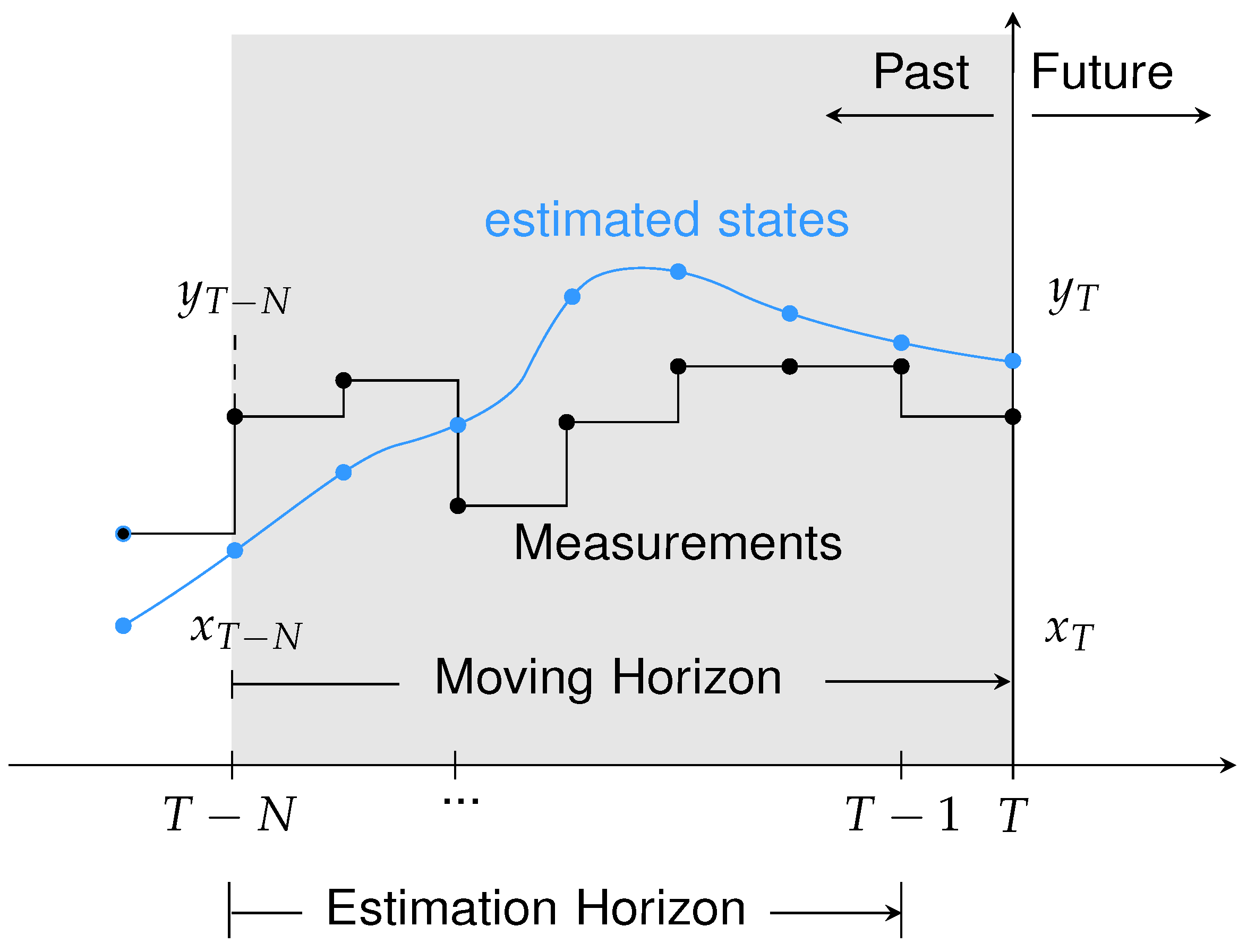
Figure 2.
Graphical abstract.
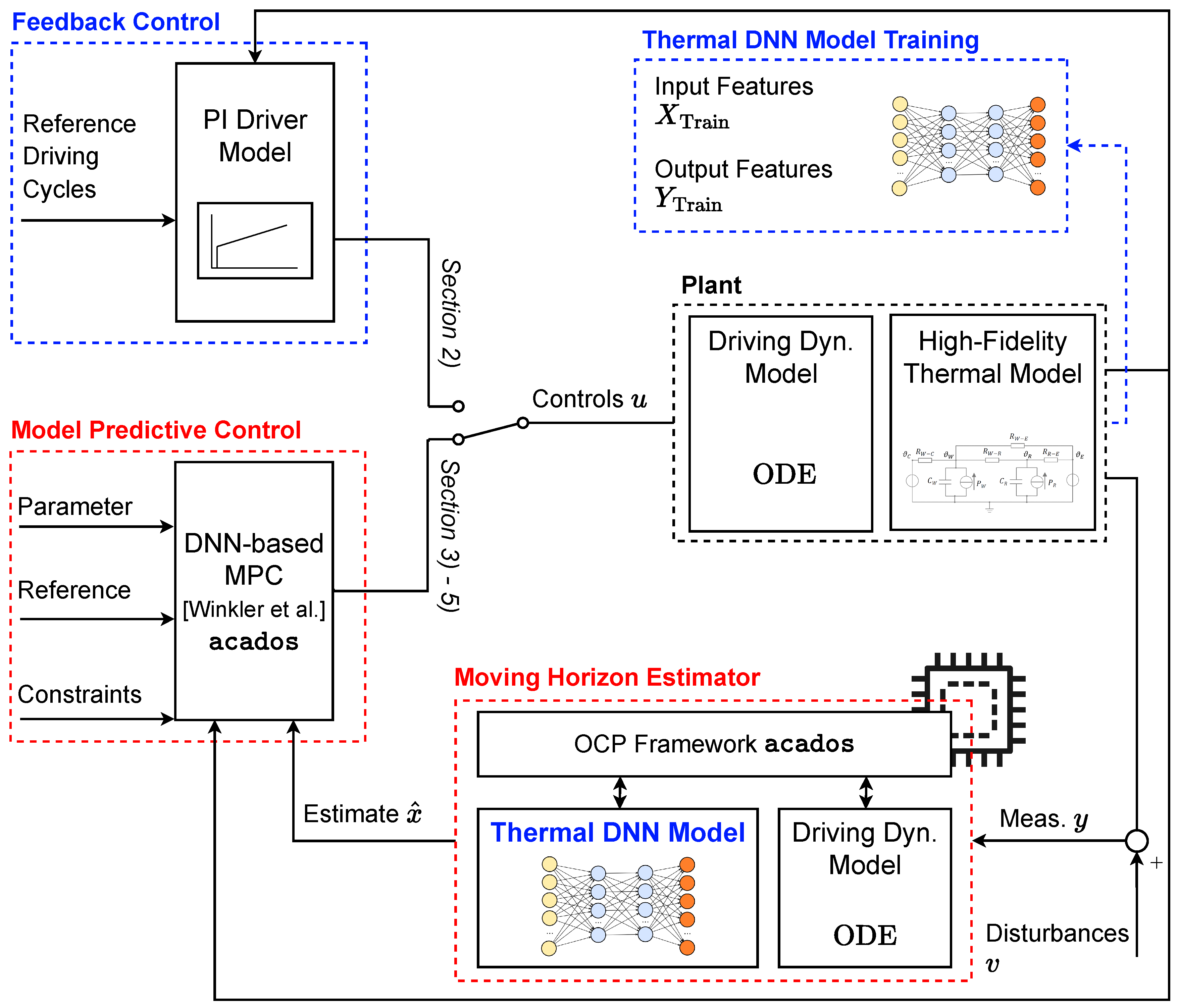
Figure 3.
Long Short-Term Memory Unit. ⊕ Element-wise Addition, ⊗ Element-wise Multiplication, u: Input, y: Output, c: Cell State, h: Hidden State, : Sigmoid Function, : Hyperbolic Tangent Function.
Figure 3.
Long Short-Term Memory Unit. ⊕ Element-wise Addition, ⊗ Element-wise Multiplication, u: Input, y: Output, c: Cell State, h: Hidden State, : Sigmoid Function, : Hyperbolic Tangent Function.
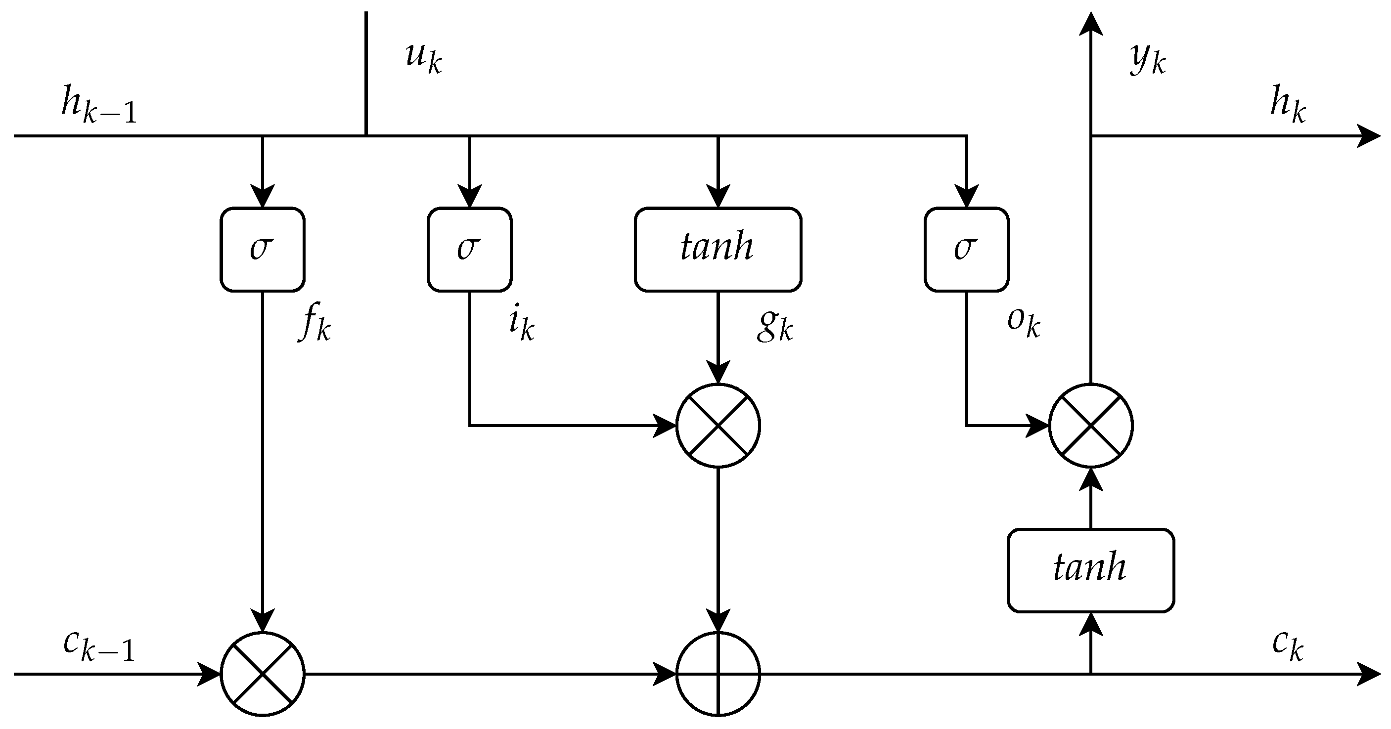
Figure 4.
Simulation and model setup for training data generation.

Figure 5.
Synthetic data generation for vehicle speed and electric machine winding temperature, utilizing multiple drive cycles.
Figure 5.
Synthetic data generation for vehicle speed and electric machine winding temperature, utilizing multiple drive cycles.
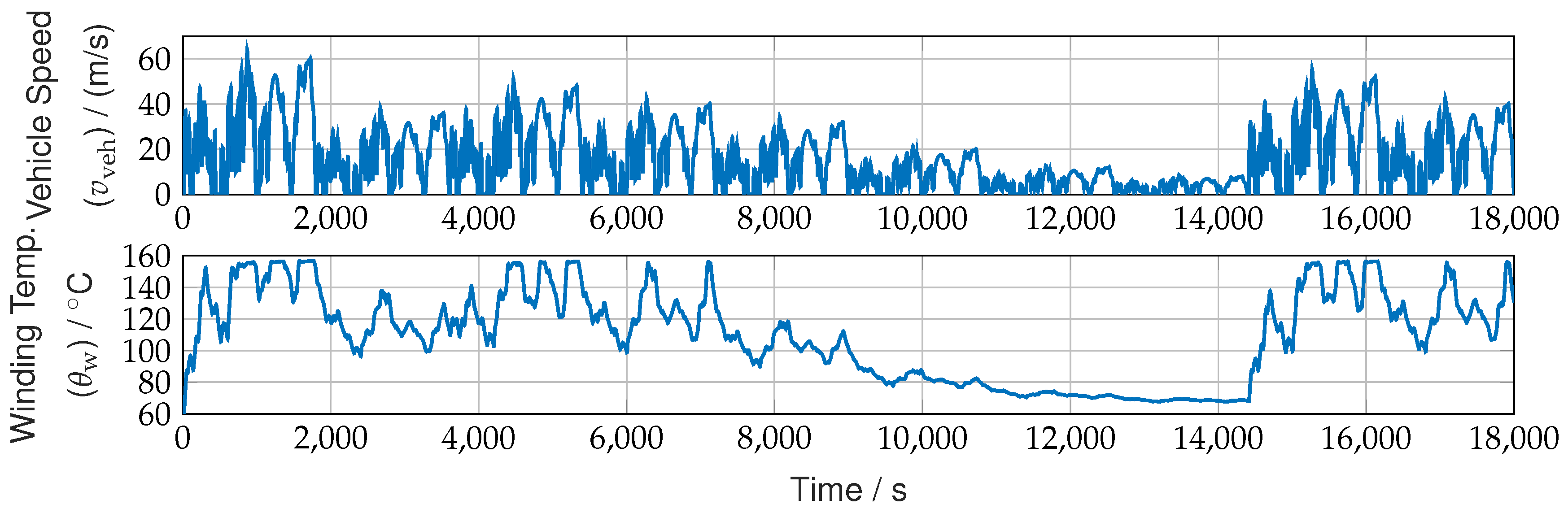
Figure 6.
LSTM artificial neural network architecture using an FC layer. LSTM: Long Short-Term Memory, FC: Fully Connected.
Figure 6.
LSTM artificial neural network architecture using an FC layer. LSTM: Long Short-Term Memory, FC: Fully Connected.
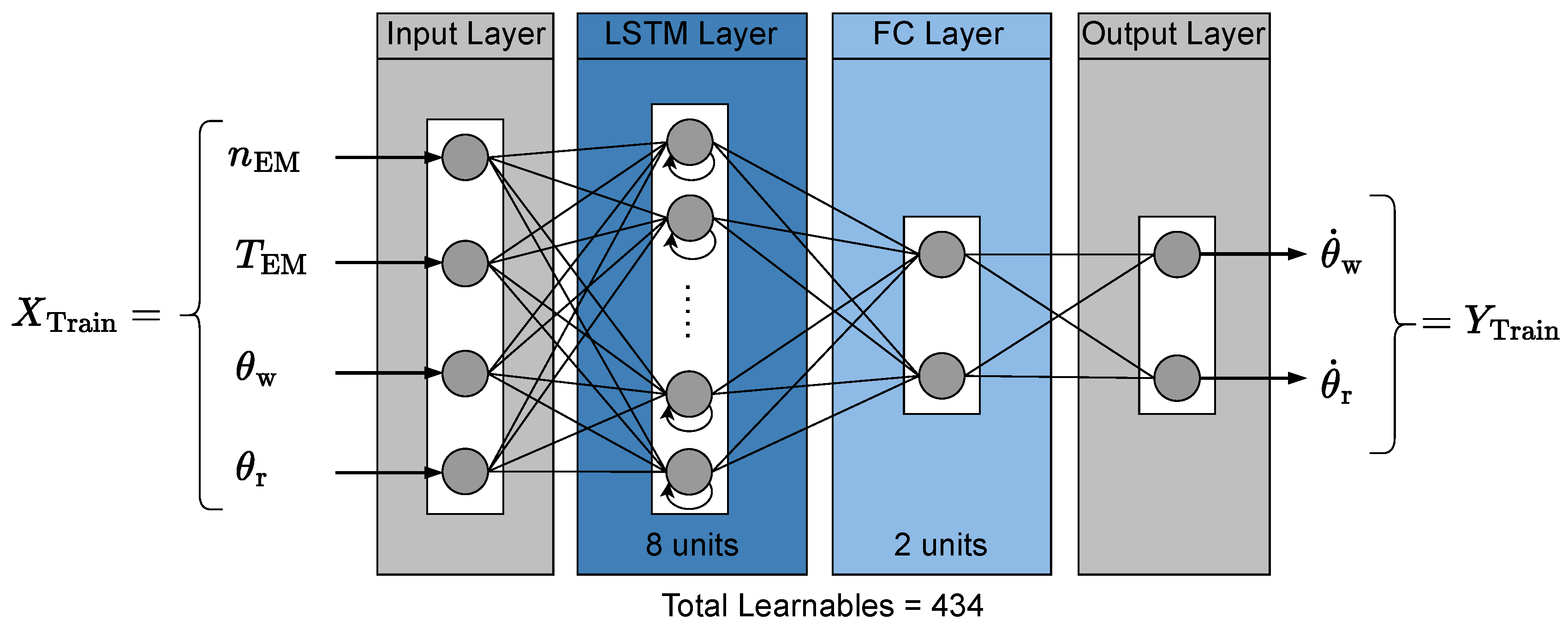
Figure 7.
Data distribution of network output gradient of electrical machine winding (upper plot) and rotor (lower plot) temperature. Training and validation dataset (80:20 split). Total data points: 180000.
Figure 7.
Data distribution of network output gradient of electrical machine winding (upper plot) and rotor (lower plot) temperature. Training and validation dataset (80:20 split). Total data points: 180000.
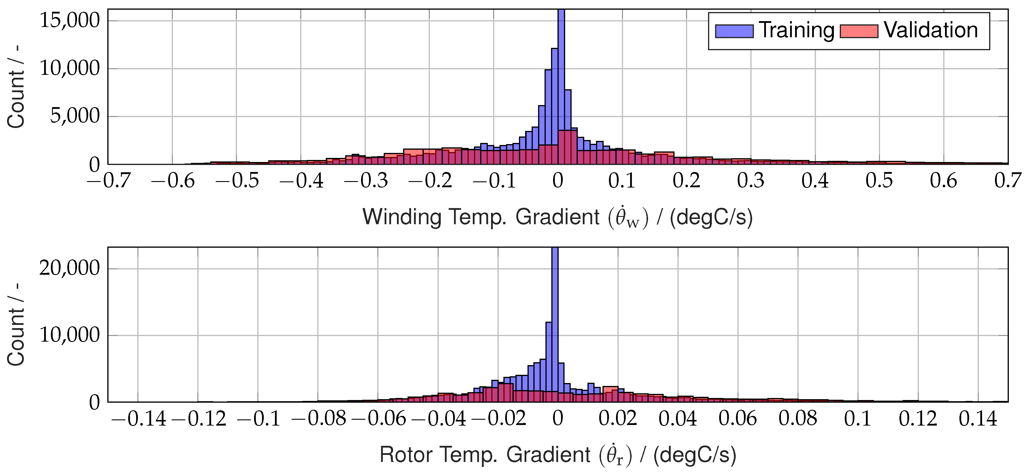
Figure 8.
Loss-Epoch plot for the neural network training. The final network is chosen according to the best training loss.
Figure 8.
Loss-Epoch plot for the neural network training. The final network is chosen according to the best training loss.
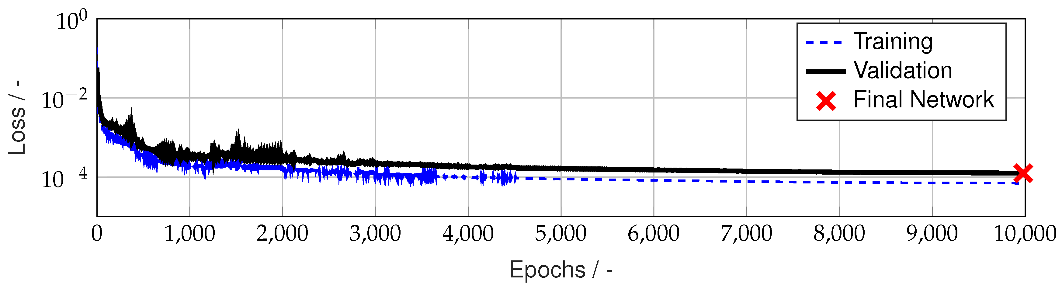
Figure 9.
Predicted neural network outputs vs. the actual ground truth data for both network outputs for unseen test dataset, gradients of winding and rotor temperature of the electric machine.
Figure 9.
Predicted neural network outputs vs. the actual ground truth data for both network outputs for unseen test dataset, gradients of winding and rotor temperature of the electric machine.
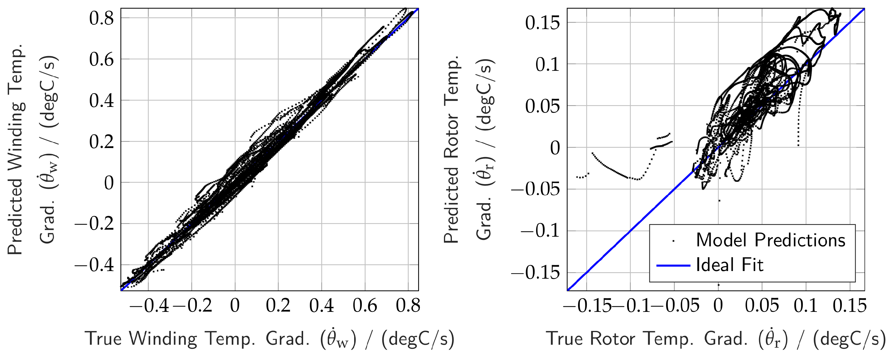
Figure 10.
Predicted neural network outputs on the unseen test (Nürburgring Nordschleife) dataset over time domain: gradients of winding and rotor temperature of the electric machine.
Figure 10.
Predicted neural network outputs on the unseen test (Nürburgring Nordschleife) dataset over time domain: gradients of winding and rotor temperature of the electric machine.
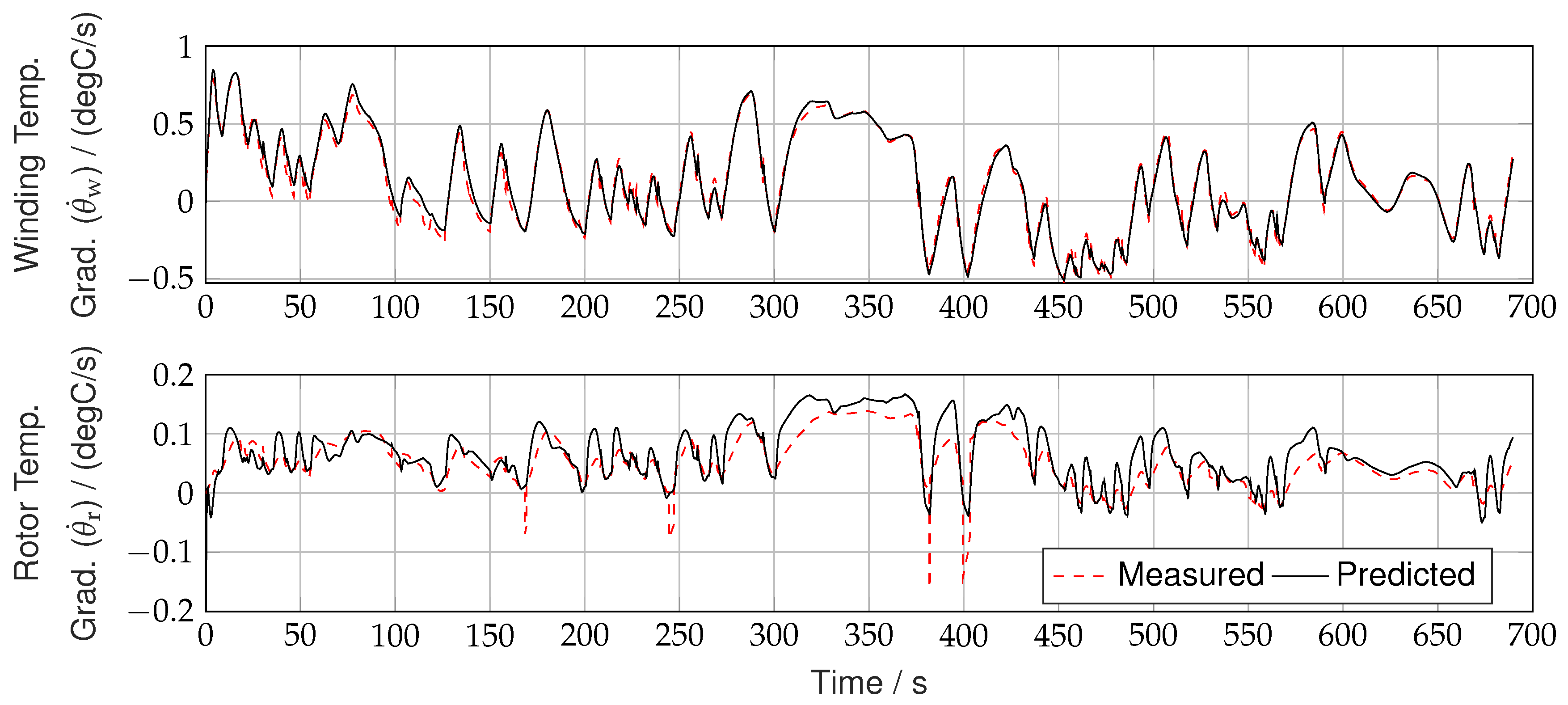
Figure 11.
Simulation and model setup for MHE application and validation.
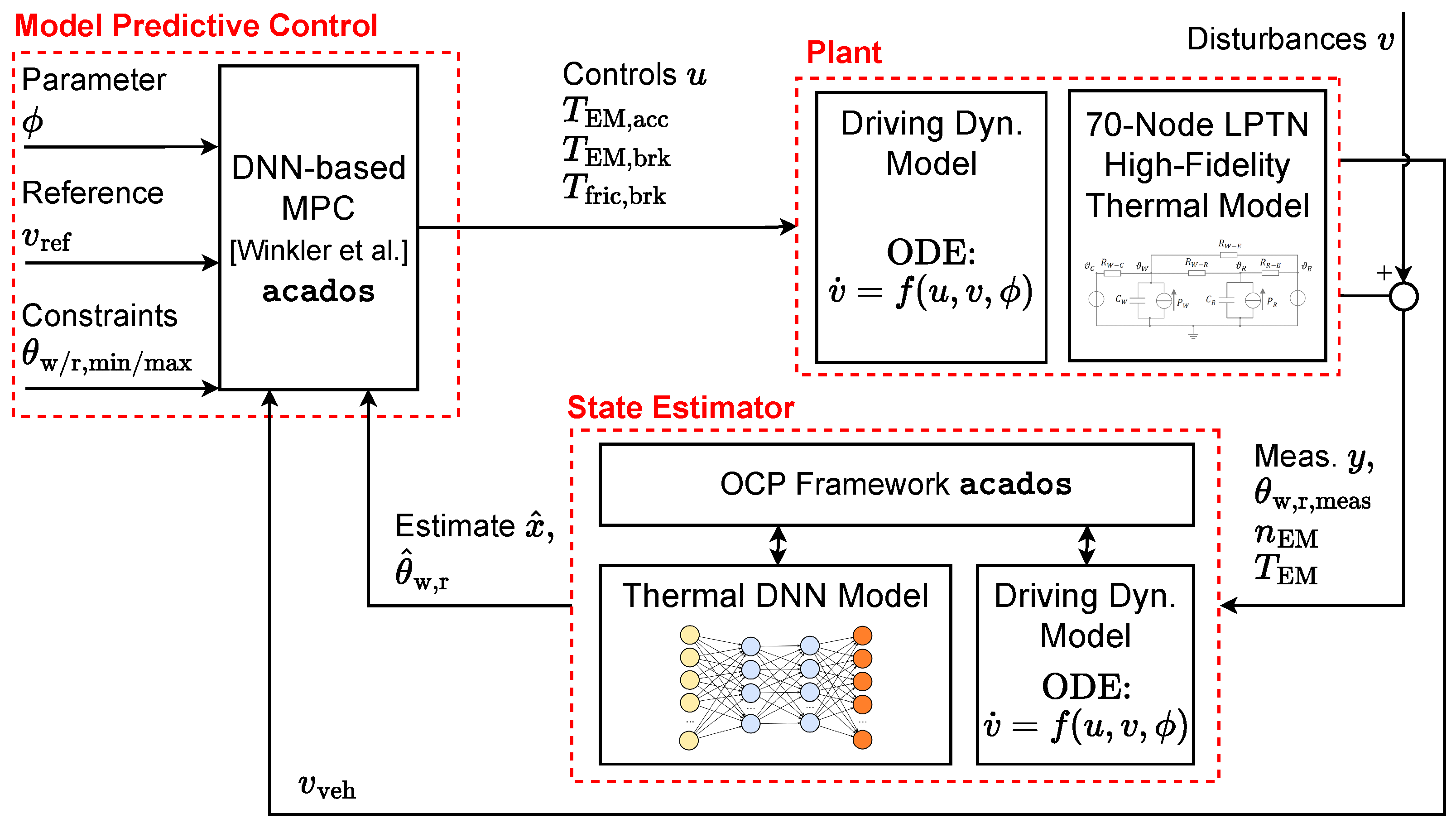
Figure 12.
Moving Horizon Estimation utilizing Long Short-Term Memory (LSTM) neural network compared to true and measured value (incl. noise) for whole drive cycle run.
Figure 12.
Moving Horizon Estimation utilizing Long Short-Term Memory (LSTM) neural network compared to true and measured value (incl. noise) for whole drive cycle run.
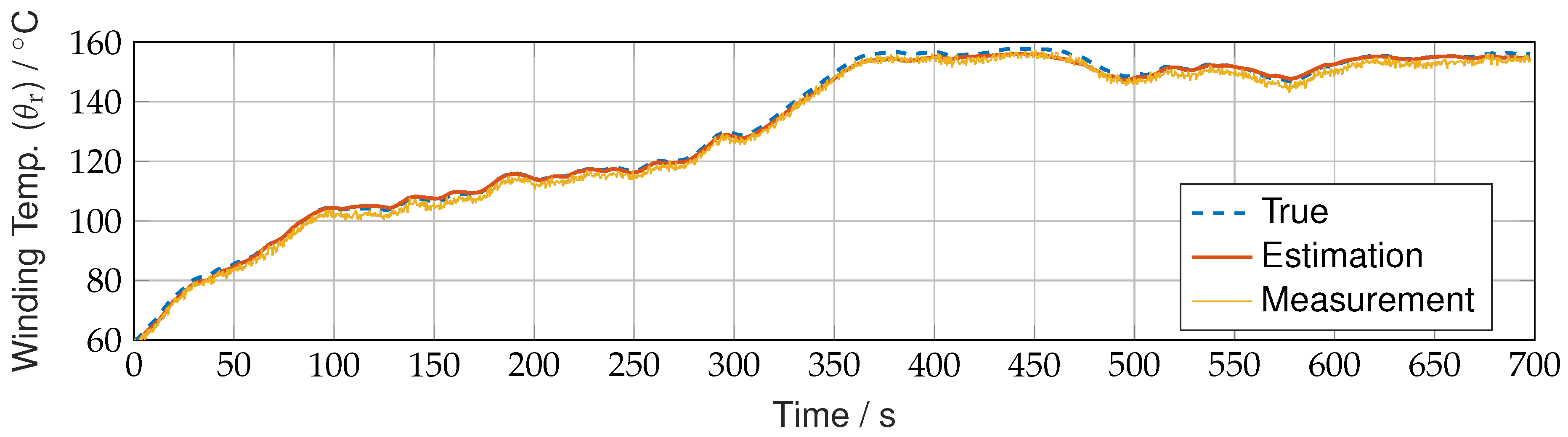
Figure 13.
Moving Horizon Estimation utilizing Long Short-Term Memory (LSTM) neural network compared to true and measured value (incl. noise) for sensible temperature range (zoom).
Figure 13.
Moving Horizon Estimation utilizing Long Short-Term Memory (LSTM) neural network compared to true and measured value (incl. noise) for sensible temperature range (zoom).
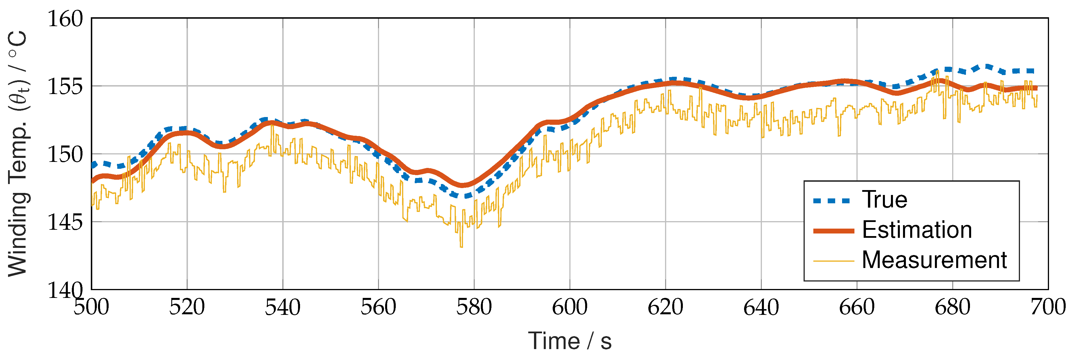
Figure 14.
Zoom plots of estimator outputs for winding temperature compared to true and measured value (incl. noise) with heavy failure injection for robustness investigation.
Figure 14.
Zoom plots of estimator outputs for winding temperature compared to true and measured value (incl. noise) with heavy failure injection for robustness investigation.
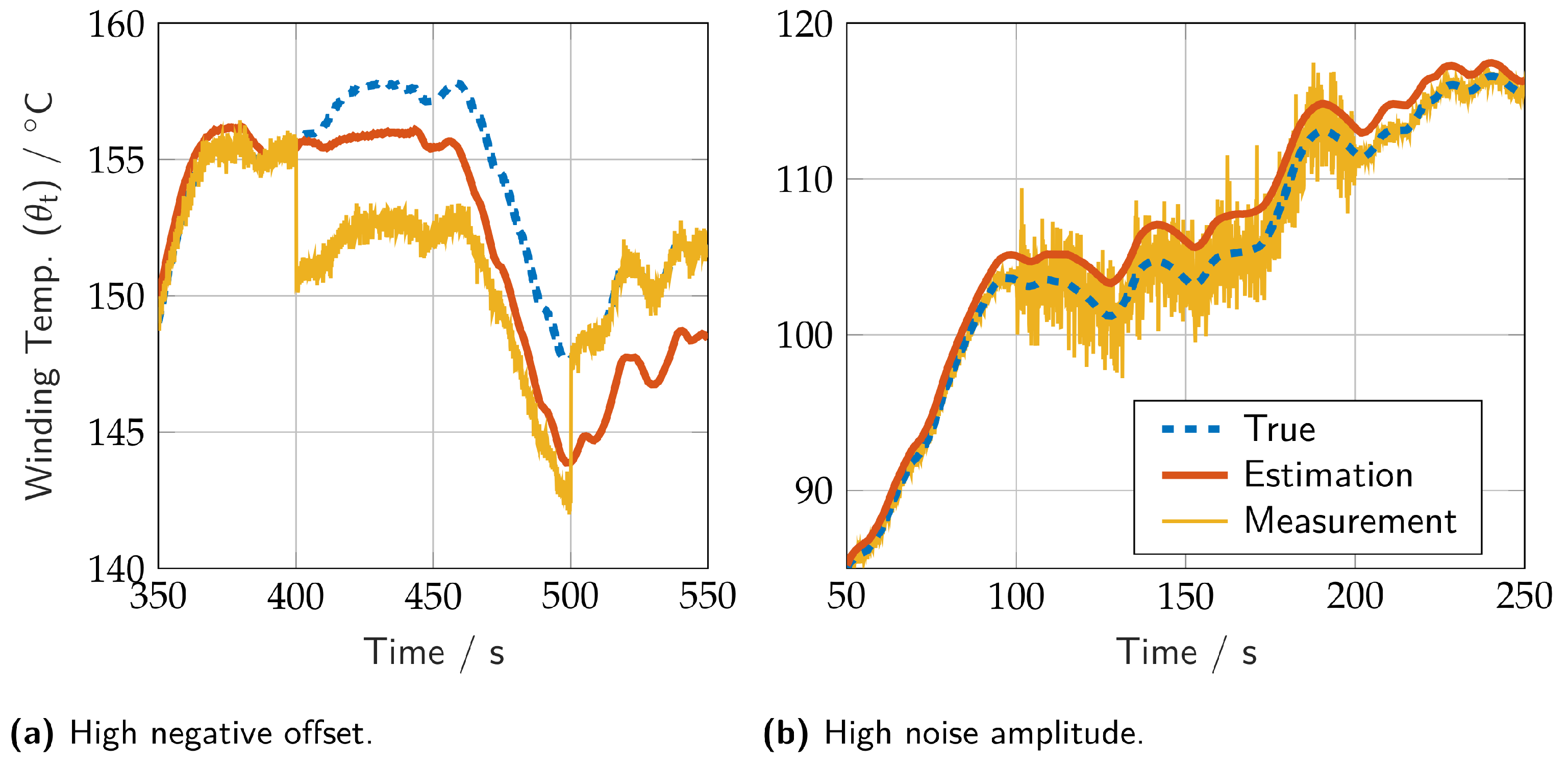

Table 1.
Training hyperparameter settings
| Hyperparameter | Value |
|---|---|
| Max epoch | 10000 |
| Optimizer | Adam |
| Mini-batch size | 512 |
| Initial learning rate | 0.02 |
| Learn rate schedule | Piecewise drop by 25% every 500 epochs |
| L2 regularization | 0.1 |
| Validation frequency | 10 |
Table 2.
Deep neural network prediction performance metrics on unseen test dataset. MAE: Mean Absolute Error, MSE: Mean Squared Error, RMSE: Root MSE, NRMSE: Normalized RMSE.
Table 2.
Deep neural network prediction performance metrics on unseen test dataset. MAE: Mean Absolute Error, MSE: Mean Squared Error, RMSE: Root MSE, NRMSE: Normalized RMSE.
| Metric | ||
|---|---|---|
| MAE / (degC/s) | 0.0288 | 0.0210 |
| MSE / (degC/s)2 | 0.0014 | 0.0008 |
| RMSE / (degC/s) | 0.0373 | 0.0282 |
| NRMSE / - | 2.77% | 9.39% |
Table 3.
Tuning parameters for Optimal Control Problem
| Symbol | Parameter | Value |
|---|---|---|
| Minimum winding and rotor temperature | 0 °C | |
| Maximum winding and rotor temperature | 155 °C | |
| Weighting matrix of the arrival cost | diag(1, 1) | |
| Q | Weighting matrix of mapped states | |
| R | Weighting matrix of controls | |
| N | Estimation horizon | 15 |
| Timestep size | 100 ms | |
| T | Horizon length | 1.5 s |
Table 4.
Parameter settings and simulation results for embedded real-time testing of deep neural network-based moving horizon estimator.
Table 4.
Parameter settings and simulation results for embedded real-time testing of deep neural network-based moving horizon estimator.
| Parameter | Value |
|---|---|
| Timestep | 100 ms |
| Horizon length (nodes) | 15, condensed to 5 |
| Maximum number of SQP iterations | 20 |
| Maximum number of iterations within the QP solver | 100 |
| Maximum computation time per timestep | 28 ms |
| Average computation time per timestep | 5.7 ms |
Disclaimer/Publisher’s Note: The statements, opinions and data contained in all publications are solely those of the individual author(s) and contributor(s) and not of MDPI and/or the editor(s). MDPI and/or the editor(s) disclaim responsibility for any injury to people or property resulting from any ideas, methods, instructions or products referred to in the content. |
© 2025 by the authors. Licensee MDPI, Basel, Switzerland. This article is an open access article distributed under the terms and conditions of the Creative Commons Attribution (CC BY) license (http://creativecommons.org/licenses/by/4.0/).
Copyright: This open access article is published under a Creative Commons CC BY 4.0 license, which permit the free download, distribution, and reuse, provided that the author and preprint are cited in any reuse.


